arX

iv:h

ep-t

h/99

1208

6v3

30

Dec

199

9

hep-th/9912086

Duality Relations

Among Topological Effects In String Theory

Edward Witten ∗

Physics Department, California Institute of Technology, Pasadena CA 91125 USA

and

CIT-USC Center for Theoretical Physics, Univ. of Southern California, Los Angeles CA

We explore two different problems in string theory in which duality relates an ordinary

p-form field in one theory to a self-dual (p + 1)-form field in another theory. One prob-

lem involves comparing D4-branes to M5-branes, and the other involves comparing the

Ramond-Ramond forms in Type IIA and Type IIB superstring theory. In each case, a

subtle topological effect involving the p-form can be recovered from a careful analysis of

the quantum mechanics of the self-dual (p+ 1)-form.

∗ On leave from Institute for Advanced Study, Princeton NJ 08540

December, 1999

1. Introduction

The purpose of this paper is to explore how certain relatively subtle topological effects

in string theory and M -theory transform into each other under dualities. We will look at

two cases that are rather similar and can be treated in rough parallel:

(1) The “U(1) gauge field” on the world-volume of a Type II D-brane is actually better

described as a Spinc structure (assuming, as we generally will in the present paper, that

the background Neveu-Schwarz three-form field H is topologically trivial). This effect,

which first showed up in a detailed example [1], has a natural interpretation in K-theory

[2,3] and can be demonstrated by studying global anomalies for elementary strings ending

on the D-brane [4]. The effect exists for Type IIA and IIB Dp-branes for several values

of p. The problem we will study arises in the case of a Type IIA D4-brane. Such a brane

can arise upon compactifying an M5-brane on a circle, in which case the “gauge field” of

the D4-brane arises by compactifying the chiral two-form (with self-dual curvature) on the

M5-brane. It must somehow be possible to deduce the Spinc nature of the D4 gauge field

from some property of the chiral two-form of the M5-brane.

(2) The Ramond-Ramond four-form field strength G4 of Type IIA superstring theory

does not, in general, obey conventional Dirac quantization. Under certain conditions [5],

there is a gravitational correction to the quantization law, and the periods of G4 are half-

integral. Type IIA superstring theory on a spacetime X = S1×Y is T -dual to Type IIB on

the same spacetime. The T -duality maps the relevant part of G4 to the self-dual five-form

G5 of Type IIB on S1 × Y . Hence, in this situation, it must be possible to deduce the

nonintegrality of the G4 periods from some property of the dynamics of G5.

What these examples have in common is that on one side of the relation, one considers

a field (the “gauge field strength” on the D4-brane, or the four-form of Type IIA) whose

periods are shifted from conventional Dirac quantization by a gravitational correction. On

the other side of the relation is a self-dual Bose field of one degree higher (the three-form

of the M5-brane, and the five-form of Type IIB) in a related theory. We must somehow

deduce the gravitational correction in the lower dimension from the quantum mechanics

of the self-dual field in the higher dimension.

The quantum mechanics of a self-dual field is quite subtle and has been studied from

many points of view, a sampling being [6-29]. Recent work has included construction of

brane Lagrangians at least locally [20,24,25] and construction of manifestly supersymmetric

and kappa-symmetric equations of motion for multiplets including the self-dual fields [26].

1

As is most familiar from the case of a chiral scalar (self-dual one-form) in two di-

mensions, and as we will review in section 3, a chiral p-form field generally has on a given

manifold several possible partition functions, determined by a choice of theta function; one

needs a recipe to pick out the right theta function in a given situation. For p > 1, this has

been demonstrated most explicitly in [30]. The right recipe for picking a theta function

depends on some physical input; for the self-dual three-form of theM5-brane, and the self-

dual five-form of Type IIB, a prescription has been given in [31]. For one specific example

above two dimensions –the self-dual three-form on T6, where the partition function turns

out to be unique (independent of the spin structure on T6) – the appropriate partition

function has been constructed and studied in detail [32]. The recipe of [31] for picking

a theta function has been related to a more classical topological invariant (the Kervaire

invariant) in [33].

An exception to the statement that the chiral p-form has several possible partition

functions arises [8] if one combines several chiral bosons using an even unimodular lattice.

Then one gets complete modular invariance and a unique partition function. This case is

very important for the heterotic string [34]. In a different case (like a single chiral scalar at

the free fermion radius, relevant to the present paper), one cannot resolve the ambiguity of

the partition function by summing over all possibilities because each candidate partition

function has slightly different anomalies, and it does not make sense to add them. In theM -

theory and Type IIB applications, the chiral p-form does not appear by itself but together

with addition fields such as fermions. The complete partition function is presumably

anomaly-free (this has not been completely demonstrated); anomaly cancellation depends

on pairing the proper (spin-structure dependent) partition function of the fermions with

the proper partition function of the chiral p-form. Thus, one must expect that the recipe

for picking a chiral p-form partition function depends on the spin structure, and this is

the case for the proposal in [31]. Once the anomalies are all canceled, it is possible, and

perhaps correct physically, to sum over spin structures.

The main goal of the present paper is to show how the quantum mechanics of the self-

dual fields gives rise, after compactification on a circle, to the effects mentioned in (1) and

(2) above. In section 2, we demonstrate the phenomena in special cases in which detailed

general theory is not needed. In the rest of the paper, we proceed more systematically. In

section 3, we recall some important facts about p-form quantum mechanics. In sections 4

and 5, we make the theory in [31] more concrete for the situation of interest and use it to

deduce what we need.

2

The first of our two problems described above is somewhat reminiscent of the problem

of relating the mechanism of M5-brane normal bundle anomaly cancellation [35] with the

corresponding mechanism in Type IIA [31]. The relation between them has been analyzed

recently [36].

2. Reduction To Chiral Scalar

The goal in the present section is to verify that the phenomena mentioned in the

introduction work out correctly in some simple cases in which we can do this without

many technicalities. This will perhaps satisfy the curiosity of some readers, and may give

others the courage needed to persevere through the technicalities of the rest of the paper.

M5-Brane Wrapped On A Circle

We first consider the relation of theM5-brane to the D4-brane. Our goal is to analyze

the M5-brane on a world-volume V = S × R, where R is an oriented five-manifold and S

is a circle with a supersymmetry-preserving spin structure. To do this in general will be

the goal of section 5, but things are much simpler in the case R = S ×R′, with S another

circle and R′ a four-manifold. The simplicity will arise because in this special case, we do

not need to understand chiral p-forms fields of p > 0; we can deduce what we need from

familiar (though subtle) facts about chiral scalars.

Though we could treat an arbitrary R′, it will suffice for illustration to take R′ = CP2.

Thus, the fivebrane world-volume will be V = Σ×CP2 where Σ = S × S is a product of

circles; the spin structure on S preserves supersymmetry but either choice may be made

on S. The nontrivial cohomology group of CP2 (apart from dimensions zero and four) is

H2(CP2;Z) = Z. (2.1)

The generator of H2(CP2;Z) is a self-dual form ω that obeys

∫

CP1

ω = 1,

∫

CP2

ω ∧ ω = 1. (2.2)

Here CP1 is a linearly embedded subspace of CP2 and generates H2(CP2;Z).

We suppose that theM -theory spacetime is X = Σ×C, where C is a nine-dimensional

spin-manifold in which CP2 is embedded. M -theory on this spacetime is equivalent to

Type IIA on X ′ = S × C; the M5-brane corresponds to a D4-brane wrapped on R =

3

S × CP2. R is not a spin manifold, since CP2 is not. As a result, according to [4], the

field strength F of the “U(1) gauge field” on the D4-brane does not obey conventional

Dirac quantization. Rather, ∫

CP1

F

2π= n+

1

2, (2.3)

with integer n.

The gauge field on the D4-brane arises by dimensional reduction from the chiral two-

form b on the M5-brane. We want to know how (2.3) arises from the theory of a chiral

two-form. We consider a limit in which the radii of S and S are much greater than the

size of the CP2. In this case, the physics on the M5-brane reduces to an effective two-

dimensional theory on Σ = S × S. In fact, the field b reduces (by the ansatz b = ωφ)

to a chiral scalar φ in two dimensions. φ appears at the self-dual or free fermion radius1;

the φ field is hence equivalent quantum mechanically to a complex fermion ψ of positive

chirality.

The ψ field propagates on the Riemann surface Σ, and the partition function of ψ

depends on a choice of spin structure on Σ. So to describe the physics, we need to know

the effective spin structure on Σ in the low energy theory, given the underlying choice of

spin structure on the M -theory spacetime X = Σ×C. Since choosing a spin structure on

X is equivalent to choosing a spin structure on Σ and choosing one on C, in the microscopic

M -theory description a spin structure was chosen on Σ at the beginning. In fact, as we

noted above, we are interested in the case that this spin structure is the product of the

supersymmetric spin structure on S and any desired spin structure on S. It is natural

to guess that the effective spin structure on Σ in the low energy theory is just the spin

structure on Σ that we start with microscopically. This assertion almost follows just from

the fact that the map from the microscopic to the macroscopic spin structure must be

1 In general, if the M5-brane is compactified to two dimensions on a four-manifold R′, the

chiral two-form reduces to a set of two-dimensional scalars with momentum lattice given by the

two-dimensional cohomology lattice of R′. For R′ = T4, this assertion is built into the detailed

computation in [32]. For R′ = CP2, the lattice is one-dimensional, generated by a vector ω with

ω2 = 1; this is the lattice of a chiral boson with the free-fermion radius. (Depending on how R′

is embedded in the full spacetime, some of the conservation laws associated with the momentum

lattice may be violated by instantons constructed from membranes with boundary on R′. This

phenomenon is irrelevant for determining the fivebrane partition function in the large volume

limit.)

4

invariant under the action of SL(2,Z) on Σ, and can be verified using the techniques of

sections 4 and 5.

In the theory of a D4-brane on S×CP2, with S regarded as the “time” direction, the

flux (2.3) can be interpreted as a conserved charge. Going back to the self-dual three-form

theory on the M5-brane worldvolume V = S × S × CP2, this flux is interpreted as the

integral of the self-dual three-form T (which is the curvature of the chiral two-form b,

defined by T = db) over S × CP1. In terms of the ansatz b = ωφ, we have T = ω ∧ dφ,and the conserved charge is

q =

∫

S×CP2

ω ∧ dφ2π

=

∮

S

dφ

2π. (2.4)

In the free fermion description, dφ/2π becomes ψψ and the charge is the conserved fermion

number

q =

∮

S

ψψ. (2.5)

Now, since the fermions on S are in the supersymmetric spin structure, both ψ and ψ

have a single zero mode on S. The quantization of the zero modes gives rise, in a way

that is familiar from the Ramond sector of superstrings, to a two-fold degeneracy of the

ground state. The ground states have fermion number q = ±1/2, and all excited states

have half-integral eigenvalues of q. Since q is interpreted in the Type IIA description as the

flux in (2.3), we have explained the half-integrality of that flux starting with the theory of

the self-dual three-form on the M5-brane.

It is also instructive to consider, in a similar fashion, a case in which the D4-brane

is wrapped on a five-manifold R that does not have a Spinc structure, so that the theory

should be inconsistent. Such a case is obtained by takingR to be not a product S×CP2 but

a CP2 bundle over S in which the fiber undergoes complex conjugation in going around S.

Complex conjugation reverses the sign of ω and so acts on φ by φ→ −φ. The periods of φthus must change sign in going around S, but since they are half-integral, this is impossible.

This is the inconsistency. But what does it look like in the free fermion description? From

this point of view, φ→ −φ is ψ ↔ ψ. Alternatively, if ψ = (ψ1 + iψ2)/√2 with Majorana-

Weyl fermions ψ1, ψ2, it is

ψ1 → ψ1, ψ2 → −ψ2. (2.6)

Both ψ1 and ψ2 couple to the supersymmetric spin structure on S, and in view of (2.6),

they see opposite spin structures on S. So ψ1 and ψ2 together have precisely one zero

5

mode on S × S. Having an odd number of fermion zero modes means that the partition

function vanishes, and that this vanishing cannot be lifted by insertions of local operators

(a fermionic operator will not have an expectation value once we average over spatial

rotations). It should be interpreted as a kind of global anomaly. We will argue in section

5.1 that the M5-brane has such an inconsistency on S ×R whenever R is not Spinc.

Analog For Type IIB

Now let us briefly discuss the analogous issues in the other case mentioned in the

introduction.

Our goal is to compare topological effects in Type IIB and Type IIA superstring

theory on S × Y , with S a circle and Y a nine-dimensional spin manifold. But a shortcut

along the above lines is possible for the special case Y = S × Y ′, with S another circle

and Y ′ an eight-dimensional spin manifold. So we consider Type IIB superstring theory

on S × S × Y ′, with the supersymmetric spin structure on the first factor.

For illustration, we consider the case that Y ′ = HP2. The only nontrivial cohomology

group of this manifold is H4(HP2;Z) = Z. The generator is a self-dual four-form ω such

that ∫

HP1

ω = 1,

∫

HP2

ω ∧ ω = 1. (2.7)

Here HP1 is a linearly embedded subspace of HP2 and generates H4(HP2;Z). HP2 is a

spin manifold, so its first Pontryagin class p1 is divisible by 2, and λ = p1/2 obeys

∫

HP1

λ = 1. (2.8)

In fact, λ is just ω.

We can repeat much of what we have already seen. In compactification on S×S×HP2,

with the last factor much smaller than the first two, the chiral four-form C4 of Type IIB

superstring theory reduces at long distances (via an ansatz C4 = ωφ) to a chiral scalar

φ on S × S. φ can be expressed in terms of free fermions, and by the same reasoning as

above, if we regard S as the “time” direction, then the conserved charge

q =

∮

S

dφ

2π(2.9)

takes half-integral values. One can think of q more microscopically as

q =

∮

S×HP1

G5

2π(2.10)

6

where G5 = dC4 is the gauge-invariant self-dual five-form of Type IIB.

Now we consider a T -duality transformation on the first circle S. This maps Type

IIB superstring theory to Type IIA, and the modes of G5 that appear in the integral in

(2.10) are mapped to G4, the Ramond-Ramond four-form field strength of Type IIA. In

the Type IIA description, q becomes

q =

∫

HP1

G4

2π. (2.11)

Thus, to account for the half-integrality of q from the Type IIA point of view, we must

explain why G4 has half-integral periods in this situation.

But this is a consequence of (2.8). The general formula is indeed [5]

∫

U

G4

2π=

1

2

∫

U

λ+ integer, (2.12)

for any four-cycle U in a Type IIA spacetime. In view of (2.8), this is equivalent to half-

integrality of q. Thus, we have succeeded, in this situation, in reconciling the gravitational

shift in the quantization law of the four-form in Type IIA with the subtleties of the self-dual

five-form of Type IIB.

For a more complete study of these problems, where we compactify on only one circle

and not two, we need to delve into the theory of chiral p-form fields for p > 0. This will

be the subject of sections 4 and 5. But first we must recall some additional aspects of the

quantum mechanics of self-dual p-forms, starting with the one-form case.

3. Quantum Mechanics Of Self-Dual p-Forms

Before looking at our specific problem, we need some more background on chiral

p-forms.

In constructing the quantum mechanics of an ordinary (not self-dual) p-form field on a

manifold M , one sums over all periods in Hp(M ;Z). That is not so for a self-dual p-form.

In fact, it is impossible to impose any classical quantization law at all on the periods

of a self-dual p-form. To illustrate this, let Σ be a two-torus constructed as C/Λ, where

C is the complex z-plane, and Λ is a lattice generated by complex numbers 1 and τ (with

Im τ > 0). Let A be a cycle in Σ that lifts in C to a path from 0 to 1, and let B be a cycle

that lifts to a path from 0 to τ . Let λ be a self-dual one-form. Then λ = c dz for some

7

complex constant c. If we want, for example,∫Aλ/2π to be integral, we need c ∈ 2πZ,

while requiring∫Bλ/2π to be integral puts an entirely different condition on c.

What happens instead is that a self-dual p-form must be treated quantum mechan-

ically; one cannot treat its periods classically. The partition function of such a field is

written as a sum over only half the periods. For illustration, let us consider an example

[8] that is extremely important in string theory: a collection of 8k chiral bosons φi in two-

dimensions, for some integer k, associated with an even unimodular lattice Γ with positive

definite intersection form ( , ). We set λi = dφi. The partition function in genus one is as

follows. Let Σ be as above and q = exp(2πiτ). Then the partition function of the chiral

boson theory on Σ is

Z(q) =

∑w∈Γ q

(w,w)/2

η(q)8k(3.1)

with η the Dedekind eta-function. In this formula, the partition function is constructed as

a sum over a single set of periods – the periods wi =∫Aλi/2π, which are the components

of a single lattice vector w ∈ Γ. In a Hamiltonian framework with A regarded as the spatial

cycle and B as time, the A-periods label the winding (or by self-duality the momentum)

states; the theta function in the numerator of (3.1) comes from the sum over these states.

Of course, the choice of the particular cycle A is not uniquely determined. The partition

function is SL(2,Z)-invariant; by an SL(2,Z) transformation, one could replace the cycle

A by nA+mB for any relatively prime integers n,m.

Intuitively, we may think of two periods∫Aλ and

∫A′λ as commuting if and only

if the intersection number A ∩ A′ is zero. There is no way to simultaneously measure

noncommuting periods. The partition function is constructed as a sum over a maximal set

of commuting periods.

The example relevant to the present paper is slightly more subtle: it is the case that

the chiral bosons φi are derived from a lattice Γ that is unimodular, but not even. In fact,

the prototype for us is a single chiral boson at the free fermion radius, that is to say Γ is a

one-dimensional lattice generated by a vector ω with (ω, ω) = 1. In this case, there is not

a single partition function; rather (as is apparent from the description by free fermions)

there is a partition function for each choice of spin structure. It is instructive to examine

these partition functions. They are conveniently written in terms of standard functions as

Z

[θφ

](z|τ) =

ϑ

[θφ

](z|τ)

η(τ), (3.2)

8

where θ and φ are 0 and 1/2 and z is an extra variable included to represent the coupling

to a background gauge field. The partition function in the absence of this field is obtained

by setting z = 0. The functions in the numerator on the right hand side are called theta

functions with characteristics. They are explicitly

ϑ

[00

](z|τ) =

∑

n∈Z

qn2/2 exp(2πinz)

ϑ

[0

1/2

](z|τ) =

∑

n∈Z

(−1)nqn2/2 exp(2πinz)

ϑ

[1/20

](z|τ) =

∑

n∈Z+1/2

qn2/2 exp(2πinz)

ϑ

[1/21/2

](z|τ) = i

∑

n∈Z+1/2

(−1)n+1/2qn2/2 exp(2πinz).

(3.3)

We have written these theta functions as sums over the A-period n =∫Adφ/2π. By

SL(2,Z), one could instead write each of these theta functions as a sum over any other

chosen period of dφ. While ϑ

[1/21/2

], which corresponds to the odd spin structure, is

SL(2,Z)-invariant (up a a c-number multiple that reflects the modular weight plus an

anomalous phase), the others are permuted by SL(2,Z), so if one chooses to write ϑ

[00

],

for example, with a different choice of the period, one might have to use the formula for

ϑ

[1/20

].

In constructing the theta function as a sum over the values of the A-period n, this

period is integral for θ = 0 and half-integral for θ = 1/2. Therefore the answer to the

question of whether a given period of the self-dual one-form is integral or half-integral

depends on the choice of theta function. On the other hand, φ determines the sign factors

in the sum over the A-periods. A configuration with a given value of the A-period n is

weighted by a sign +1 if φ = 0 and by a sign (−1)n (or (−1)n+1/2 if n is half-integral) if

φ = 1/2.

Now, we want to describe the theta functions in a way that generalizes to higher genus

surfaces and also to self-dual p-forms of p > 1. We will define a Z2-valued function Ω(x)

on the lattice Λ as follows.2 For the lattice points 1 and τ , we set

Ω(1) = (−1)2φ, Ω(τ) = (−1)2θ. (3.4)

2 In [31], this function was called H(x), but I want to avoid notational clashes with the three-

form field H of string theory and Hi(M) for cohomology groups.

9

We extend Ω to a function on the whole lattice by requiring

Ω(x+ y) = Ω(x)Ω(y)(−1)(x,y), (3.5)

where (x, y) = −(y, x) is the intersection form on the lattice Λ. For example, this definition

gives

Ω(1 + τ) = −Ω(1)Ω(τ), (3.6)

since 1 and τ correspond to the cycles A and B, whose intersection number is 1. (3.5)

is the basic formula. Theta functions are in natural one-to-one correspondence with Z2-

valued functions on the lattice that obey this relation. Given Ω, the characteristics θ, φ are

extracted from (3.4) and used to write the explicit formulas for the theta functions that

we gave above.

Let Λ1 and Λ2 be, respectively, the sublattices of Λ generated by 1 and by τ ; we call

these the A-lattice and the B-lattice. As we saw above, a configuration with A-period

n contributes to the theta function (in the representation of that function as a sum over

the A-periods) with a sign 1 or (−1)n depending on φ. (3.4) means that Ω(x) for x in

the A-lattice is simply the sign factor with which a configuration of A-period n = x (or

n = x+ 1/2) contributes to the theta function. Likewise, we saw above that θ determines

whether the A-periods are integral or half-integral, and thus this is determined by Ω(x)

for x in the B-lattice.

The classification of theta functions by Z2-valued functions Ω(x) extends beyond the

genus one case that we have just considered: level one theta functions of any lattice Λ with

unimodular antisymmetric form ( , ) and a metric for which this form is positive and of

type (1, 1) are classified by functions Ω obeying (3.5). This fact has a differential-geometric

explanation that was reviewed in [31]. (The basic idea is that such an Ω determines a line

bundle over Σ; this line bundle has up to constant multiples a unique holomorphic section

which is the theta function.) For our present purposes, we will simply note that the

functions Ω that obey (3.5) transform under SL(2,Z) the same way that theta functions

do. In this assertion, the sign factor (−1)(x,y) in (3.5) is essential. For example, the theta

function ϑ

[1/21/2

]associated with the odd spin structure is SL(2,Z)-invariant, so it must

be associated with a function Ω(x) that is likewise SL(2,Z)-invariant. Since θ = φ = 1/2,

this theta function has Ω(1) = Ω(τ) = −1. As SL(2,Z) can map the lattice points 1 or τ

to 1 + τ , it follows that Ω(1 + τ) must equal −1, which is what we get from (3.6).

10

To write the four theta functions by explicit formulas as in (3.3) requires a choice of

A-lattice. Some more information is needed, though, because the choice of A-lattice is

invariant under τ → τ +1, but this operation permutes the theta functions in a non-trivial

fashion. If one is also given a choice of B-lattice (and thus essentially the basis (1, τ) for

the lattice Λ), this is more than enough information to enable the writing of the explicit

formulas in (3.3). (For that, it is enough to know the B-cycles mod 2.) If one has chosen

both the A-lattice and the B-lattice, then one has an explicit SL(2,Z) transformation

τ → −1/τ that exchanges them. It exchanges θ and φ, and thus exchanges a half-integral

shift in the value of the A-period n with a sign factor by which the different values of the

A-period are weighted.

Generalization

Now let us consider the generalization to a self-dual p-form field Gp, of p possibly

bigger than 1, on a 2p-dimensional manifoldM . (For a detailed treatment via holomorphic

factorization of the partition function of a non-chiral theory, see [30].) The periods take

values in Λ = Hp(M ;Z), which for simplicity we will assume to be torsion-free. Thus

Λ is a lattice, with an antisymmetric bilinear form ( , ) of determinant 1 that is given

by the intersection pairing on M . If Λ has rank 2g, then it has has 22g distinguished

theta functions ϑ

[θφ

](z|τ) that we will introduce momentarily. The partition function of

Gp is ϑ

[θφ

](z|τ)/∆, where ∆ (analogous to η(τ) in (3.2)) is uniquely determined from

the non-zero modes of G. The subtlety comes from the choice of theta function in the

numerator.

As in the case of a one-form field, the periods of G are not all simultaneously measure-

able. The best that one can do is to pick a maximal sublattice Λ1 consisting of mutually

“commuting” periods. Λ1 is a lattice of A-periods, that is, it is a half-dimensional sub-

lattice of Λ such that (x, y) = 0 for x, y ∈ Λ1. It is convenient, though not necessary, to

pick also a complementary lattice Λ2 of B-periods. Thus, Λ = Λ1 ⊕Λ2, and (x, y) = 0 for

x, y ∈ Λ2. Picking the B-periods and A-periods gives an explicit period matrix τij = τji,

i, j = 1, . . . , g for the lattice Λ.

Once the A-cycles and B-cycles are fixed, one can write an explicit formula for the

theta functions. One picks a half-lattice vector θ ∈ 12Λ1/Λ1, and a half-lattice vector

φ ∈ 12Λ2/Λ2. The theta function with characteristics θ, φ is then

ϑ

[θφ

](zi|τ) =

∑

n∈Λ1+θ

exp

iπ

∑

ij

ninjτij + 2πini(zi + φi)

. (3.7)

11

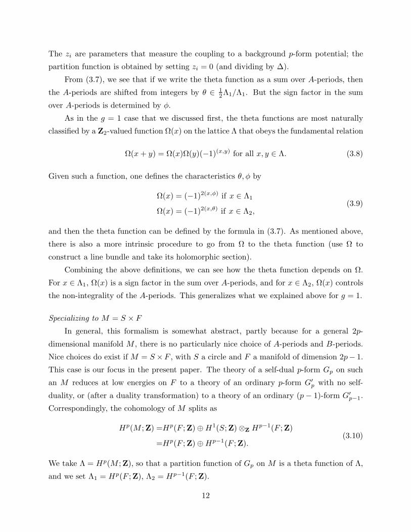
The zi are parameters that measure the coupling to a background p-form potential; the

partition function is obtained by setting zi = 0 (and dividing by ∆).

From (3.7), we see that if we write the theta function as a sum over A-periods, then

the A-periods are shifted from integers by θ ∈ 12Λ1/Λ1. But the sign factor in the sum

over A-periods is determined by φ.

As in the g = 1 case that we discussed first, the theta functions are most naturally

classified by a Z2-valued function Ω(x) on the lattice Λ that obeys the fundamental relation

Ω(x+ y) = Ω(x)Ω(y)(−1)(x,y) for all x, y ∈ Λ. (3.8)

Given such a function, one defines the characteristics θ, φ by

Ω(x) = (−1)2(x,φ) if x ∈ Λ1

Ω(x) = (−1)2(x,θ) if x ∈ Λ2,(3.9)

and then the theta function can be defined by the formula in (3.7). As mentioned above,

there is also a more intrinsic procedure to go from Ω to the theta function (use Ω to

construct a line bundle and take its holomorphic section).

Combining the above definitions, we can see how the theta function depends on Ω.

For x ∈ Λ1, Ω(x) is a sign factor in the sum over A-periods, and for x ∈ Λ2, Ω(x) controls

the non-integrality of the A-periods. This generalizes what we explained above for g = 1.

Specializing to M = S × F

In general, this formalism is somewhat abstract, partly because for a general 2p-

dimensional manifold M , there is no particularly nice choice of A-periods and B-periods.

Nice choices do exist if M = S ×F , with S a circle and F a manifold of dimension 2p− 1.

This case is our focus in the present paper. The theory of a self-dual p-form Gp on such

an M reduces at low energies on F to a theory of an ordinary p-form G′

p with no self-

duality, or (after a duality transformation) to a theory of an ordinary (p− 1)-form G′

p−1.

Correspondingly, the cohomology of M splits as

Hp(M ;Z) =Hp(F ;Z)⊕H1(S;Z)⊗Z Hp−1(F ;Z)

=Hp(F ;Z)⊕Hp−1(F ;Z).(3.10)

We take Λ = Hp(M ;Z), so that a partition function of Gp on M is a theta function of Λ,

and we set Λ1 = Hp(F ;Z), Λ2 = Hp−1(F ;Z).

12

We take the lattice of A-periods to be Λ1 and the lattice of B-periods to be Λ2. A

theta function for Λ can be constructed either as a sum over A-periods – corresponding

to the representation of the theory on F in terms of G′

p – or as a sum over B-periods –

corresponding to the representation of the theory on F in terms of G′

p−1.

No matter which representation one uses, the theta function of Λ is determined by

a choice of a suitable function Ω(x) on Λ. How to construct such a function for the

self-dual p-form fields mentioned in the introduction was explained in [31]. Once Ω is

selected, its restriction to Λ1 determines a sign factor in the sum over periods if one uses

the description of the theory in terms of G′

p, or a nonintegrality of the G′

p−1 periods in the

other description. Conversely, the restriction of Ω to Λ2 determines the nonintegrality of

G′

p periods, or a sign factor in the sum over G′

p−1.

The fact that a sign factor on one side becomes, after duality, a nonintegrality of the

periods in the other description can also be explained more microscopically in terms of

a Feynman path integral representation of the G′

p and G′

p−1 theories. More generally, in

d dimensions, a phase factor in a theory with k-form curvature Gk is always translated

after duality to a shift in periods of a dual field Gd−k . This holds for all d and k. A path

integral derivation of this fact can be found (for d = 4, k = 2, but the general case is not

essentially different) in section 4.2 of [37].

4. Systematic Analysis Of Type II Case

In attempting a systematic treatment, using the framework of [31], of the problems

mentioned in the introduction, we will begin with the second problem – understanding the

shifted quantization law of the Type IIA four-form from the quantum mechanics of the

self-dual five-form of Type IIB. This case involves fewer technicalities.

4.1. Outline

In Type IIB theory on a ten-dimensional spin manifold X , we have a four-form poten-

tial C4 with a self-dual curvature five-form G5. If we could omit the self-duality condition,

and we impose conventional Dirac quantization, then the C4-fields are classified topologi-

cally by a class x ∈ H5(X ;Z). Here x is represented in de Rham cohomology by G5/2π.

We sometimes write informally x = [G5/2π].

For an ordinary four-form field, we would construct the partition function by summing

over all choices of x (and for each choice of x, integrating over all possibilities for C4). For a

13

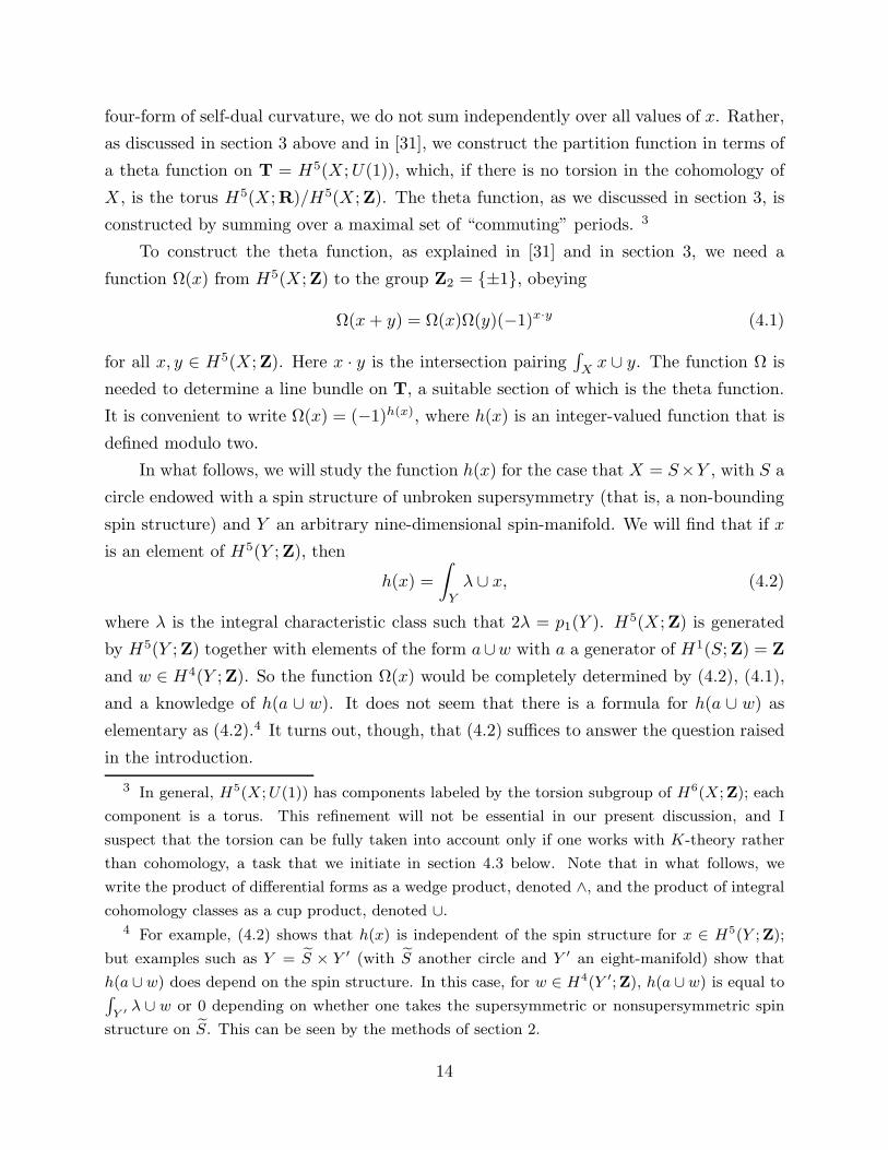
four-form of self-dual curvature, we do not sum independently over all values of x. Rather,

as discussed in section 3 above and in [31], we construct the partition function in terms of

a theta function on T = H5(X ;U(1)), which, if there is no torsion in the cohomology of

X , is the torus H5(X ;R)/H5(X ;Z). The theta function, as we discussed in section 3, is

constructed by summing over a maximal set of “commuting” periods. 3

To construct the theta function, as explained in [31] and in section 3, we need a

function Ω(x) from H5(X ;Z) to the group Z2 = ±1, obeying

Ω(x+ y) = Ω(x)Ω(y)(−1)x·y (4.1)

for all x, y ∈ H5(X ;Z). Here x · y is the intersection pairing∫Xx ∪ y. The function Ω is

needed to determine a line bundle on T, a suitable section of which is the theta function.

It is convenient to write Ω(x) = (−1)h(x), where h(x) is an integer-valued function that is

defined modulo two.

In what follows, we will study the function h(x) for the case that X = S×Y , with S a

circle endowed with a spin structure of unbroken supersymmetry (that is, a non-bounding

spin structure) and Y an arbitrary nine-dimensional spin-manifold. We will find that if x

is an element of H5(Y ;Z), then

h(x) =

∫

Y

λ ∪ x, (4.2)

where λ is the integral characteristic class such that 2λ = p1(Y ). H5(X ;Z) is generated

by H5(Y ;Z) together with elements of the form a∪w with a a generator of H1(S;Z) = Z

and w ∈ H4(Y ;Z). So the function Ω(x) would be completely determined by (4.2), (4.1),

and a knowledge of h(a ∪ w). It does not seem that there is a formula for h(a ∪ w) as

elementary as (4.2).4 It turns out, though, that (4.2) suffices to answer the question raised

in the introduction.

3 In general, H5(X;U(1)) has components labeled by the torsion subgroup of H6(X;Z); each

component is a torus. This refinement will not be essential in our present discussion, and I

suspect that the torsion can be fully taken into account only if one works with K-theory rather

than cohomology, a task that we initiate in section 4.3 below. Note that in what follows, we

write the product of differential forms as a wedge product, denoted ∧, and the product of integral

cohomology classes as a cup product, denoted ∪.4 For example, (4.2) shows that h(x) is independent of the spin structure for x ∈ H5(Y ;Z);

but examples such as Y = S × Y ′ (with S another circle and Y ′ an eight-manifold) show that

h(a ∪w) does depend on the spin structure. In this case, for w ∈ H4(Y ′;Z), h(a ∪w) is equal to∫Y ′

λ ∪ w or 0 depending on whether one takes the supersymmetric or nonsupersymmetric spin

structure on S. This can be seen by the methods of section 2.

14

This comes about as follows. The use of the function Ω(x) to determine the partition

function on a general X is perhaps slightly esoteric. But this function has a more down-

to-earth interpretation if X is of the form S × Y . In this case, the theory of the self-dual

five-form G5 on X reduces on Y , at low energies, to a theory of a five-form on Y that obeys

no self-duality condition. We will call this field G′

5. As Y is nine-dimensional, the theory

of G′

5 is dual to a theory of a four-form field G′

4 on Y . G′

4 and G′

5 are the curvatures of

three-form and four-form potentials C′

3 and C′

4. The same theory on Y can be described

with either C′

3 or C′

4 as the dynamical variable.

Ω(x) has, as we have seen in section 3, the following straightforward interpretation

when X is of the form S × Y : it is a factor that must be included in the low energy path

integral for the G′

5 field on Y . To be more precise, if we regard the theory on Y as the

theory of a five-form G′

5 with flux or characteristic class x = [G′

5/2π], then performing the

path integral involves summing over x. The sum is weighted with a number of standard

factors, such as an obvious factor coming from the kinetic energy of the C′

4 field. In

addition, we must include in the sum over x the sign factor Ω(x), which according to (4.2)

is

exp

(iπ

∫

Y

λ ∪ x)

= exp

(1

2i

∫λ ∧G5

). (4.3)

On the other hand, if we represent the theory on Y by a four-form G′

4 with flux or

characteristic class u = [G′

4/2π], then performing the path integral involves summing over

u. The sign factor we must include in the path integral is in this case Ω(a ∪ u) (since the

relation between G5 and G′

4 is that the appropriate part of G5 is a ∧G4), and we will not

determine Ω(a ∪ u). In addition to this in general unknown sign factor, the path integral

over G′

4 has another interesting effect, which arises by duality from (4.3).5 As we have

discussed in section 3, and as was explained from a path integral point of view in [37],

a phase factor on one side is converted by duality into a shift on the other side. In the

present instance, since the phase in (4.3) is 12λ (times G′

5), it is converted by duality into

a shift in the periods of G′

4 by that amount: for any four-cycle U ∈ Y ,

∫

U

G′

4

2π=

1

2

∫

U

λ mod Z. (4.4)

5 And, conversely to what we are about to say, the undetermined sign factor Ω(a ∪ u) in the

G′

4 theory will by duality, if it is not trivial, induce a shift in the periods of G′

5.

15

The last formula is essentially the result that we need. The problem posed in the

introduction was to understand, starting with the quantum mechanics of the Type IIB

self-dual five-form G5, the fact that for any four-cycle U in a Type IIA spacetime X ,

∫

U

G4

2π=

1

2

∫

U

λ mod Z, (4.5)

where here G4 is the Type IIA four-form. If X = S × Y with S a circle, then components

of λ with an index tangent to S vanish topologically (since λ is a pullback from Y ), and

the interesting case of (4.5) is the case with U a four-cycle in Y . Hence the interesting

part of G4 is the part with all indices tangent to Y . In the T -duality between Type IIB

and Type IIA on S × Y , this part of G4 is related to the part of G5 of the form a ∪ G4,

with a a generator of H1(S;Z). So the relevant part of G4 is the same as G′

4, and (4.4) is

equivalent to the desired relation (4.5).

In the next subsection, we will justify the crucial formula (4.2). Then in section 4.3,

we will propose a new description of Ω(x) in K-theory which may be more useful for

understanding dualities and the role of torsion.

4.2. Evaluation Of Ω(x)

First we recall from [31] the definition of Ω(x) for a general X . We work on Z = S′×Xwhere S′ is a circle with a Neveu-Schwarz spin structure (that is, S′ is a spin boundary). We

fix a generator a′ of H1(S′;Z) = Z. For x ∈ H5(X ;Z), we set z = a′ ∪x ∈ H6(S′ ×X ;Z).

Now, ifW is any twelve-dimensional spin manifold with boundary Z over which z extends,6

we set

h(x) =

∫

W

z ∪ z (4.6)

and Ω(x) = (−1)h(x). For Ω(x) to be well-defined, h(x) must be independent modulo 2 of

the choice of W . This is so because for a closed twelve-dimensional spin manifold W (that

is, one whose boundary vanishes),∫Wz ∪ z is even for any z ∈ H6(W ;Z). (A proof of this

assertion is cited in a footnote in section 4 of [31].)

We could calculate more conveniently if we did not have to require W to be a spin

manifold. However, if we try to use the definition (4.6) without requiring W to be spin,

h(x) would not be well-defined modulo 2 because∫Wz ∪ z is not necessarily even on a

6 How to generalize the discussion if W does not exist is discussed in [31]. We also give more

general definitions of Ω(x) below and in section 4.3.

16

general twelve-manifold W . There is, however, an analogous quantity that is even in

general; it is∫W(z ∪ z + v ∪ z), where v is the (six-dimensional) Wu class of W . v can be

expressed in terms of Stieffel-Whitney classes; for our purposes, we can assume that W is

orientable, in which case the relation is v = w2 ∪ w4. Thus, we are tempted to generalize

the definition of h(x) to

h(x) =

∫

W

(z ∪ z + w2 ∪ w4 ∪ z) (4.7)

where W is now required only to be oriented. (To make sense of the second integral, z is

reduced mod 2 and the integral is understood in terms of the cup product and integration

in mod 2 cohomology.)

Some care is needed here. Though the right hand side of (4.7) is indeed even if the

boundary of W vanishes, some subtlety enters in defining the integral when W has a

nonzero boundary. An integral such as (4.7) is not a topological invariant on a manifold

with boundary unless the class that is being integrated is trivialized on the boundary; and

even if it is, the integral depends on the choice of a trivialization on the boundary. (At

the level of differential forms, this statement means that an integral∫W

Θ, where Θ is a

twelve-form, is not necessarily invariant under Θ → Θ + dΛ if Λ is nonvanishing on the

boundary.) In the case of (4.7), if we understand z near the boundary Z of W to be a

pullback from Z, then z ∪ z vanishes near the boundary for dimensional reasons, and this

trivialization is natural. We need more care with the term w2 ∪ w4 ∪ z.As z and w4 are both in general nonzero near the boundary, the only reason that

w2 ∪w4 ∪ z vanishes near the boundary is that w2 does, that is, the boundary manifold Z

is spin. A trivialization of w2 near the boundary is a choice of spin structure on Z, and

hence we will have to use the spin structure of Z in defining the integral∫Ww2 ∪ w4 ∪ z

even though at first sight the integral appears not to depend on a choice of spin structure.

A rather down-to-earth way to build in the spin structure of Z is to restrict to the case

that W is a Spinc manifold, with a Spinc structure that extends the spin structure on Z.

The Spinc structure on W determines an integral lift7 α of w2(W ) that is supported away

from the boundary of W ; to be more precise, it determines an element α of the relative

cohomology group H2(W, ∂W ;Z) that reduces to w2(W ) mod 2. Moreover, if W and W ′

are two Spinc manifolds with (oppositely oriented) boundary Z and Spinc structures that

7 A Spinc structure determines a Spinc bundle that is informally S ⊗L1/2 where S is the spin

bundle and L is a line bundle with c1(L) congruent to w2(W ) mod 2. If W is not spin, neither S

nor L1/2 exists separately, but S ⊗ L1/2 and L do. α is defined as c1(L).

17

extend the spin structure of Z, then upon gluing together W and W ′ to make a closed

twelve-dimensional Spinc manifold W , the corresponding classes α and α′ glue together to

an integral lift α of w2(W ). In fact, α is derived from the Spinc structure on W that is

obtained by gluing those on W and W ′. (Gluing α and α′ to make an integral lift α of

w2(W ) would not work for arbitrary integral lifts α and α′ of w2(W ) and w2(W′); that is

why it is important to derive α and α′ from Spinc structures that extend that of Z.)

Finally, we get our more general definition of h(x):

h(x) =

∫

W

(z ∪ z + α ∪ w4 ∪ z) . (4.8)

This is well-defined mod 2 because it is even for a closed twelve-dimensional Spinc manifold

W .

Evaluation For X = S × Y

We are ready to compute for the case that X = S × Y , with the supersymmetric (or

non-bounding) spin structure on S. We have Z = S′ ×X = S′ × S × Y .

We want to evaluate h(x) where x is an element of H5(Y ;Z). We have z = a′ ∪ x.To compute h(x), we should write Z as a boundary of a Spinc manifold W over which z

extends. We could try to take W = D′ × S × Y , where D′ is a two-dimensional disc with

boundary S′. This is not convenient because a′ does not extend over D′. Instead, we let

D be a disc with boundary S, and set W = S′ ×D× Y . The spin structure of S does not

extend over D as a spin structure, but it extends as a Spinc structure with

∫

D

α = 1. (4.9)

As z is a pullback from S′×Y , it extends overW = S′×D×Y as such a pullback. Now we

can evaluate (4.8). On dimensional grounds, since z is pulled back from S′ × Y , z ∪ z = 0.

So we need only consider the integral over S′ ×D× Y of α∪w4 ∪ z = α∪w4 ∪ a′ ∪x. Theintegral is easily done because all factors are pullbacks from one of the factors in S′×D×Y(a′ from S′, α from D, and the others from Y ). Using (4.9) and

∫S′a′ = 1, we get

h(x) =

∫

Y

w4 ∪ x =

∫

Y

λ ∪ x, (4.10)

where the two expressions are equivalent because on the spin manifold Y , λ is an integral

lift of w4. This is the promised formula (4.2).

18

4.3. K-Theory Definition Of Ω(x)

We have performed this computation in a framework [31] in which Ω(x) is defined as

a function on middle-dimensional cohomology of Type IIB. For two reasons, it seems that

the definition should be reformulated in K-theory:

(1) In view of T -dualities which relate the Ramond-Ramond (RR) forms of different

dimensions, and relate Type IIB to Type IIA, it seems unnatural to have a special for-

malism which only applies to the middle-dimensional RR form for Type IIB, and does not

apply at all for Type IIA. If we define Ω(x) in K-theory, this will automatically include

all of the RR forms of all even or all odd dimension, and may give a T -dual formalism.

(2) In view of what we now know about the RR fields, it seems unlikely that one

can correctly take into account the torsion part of the RR fluxes without using K-theory

instead of cohomology.

The rest of this section is devoted to an attempt to give a K-theory definition of Ω(x).

For Type IIA at the level of differential forms, the total RR field G = G0+G2+G4+. . .

is a sum of differential forms of all even orders. For Type IIB, one has instead a sum

G = G1 + G3 + . . . of differential forms of all odd orders. In passing to K-theory, we will

assume that for Type IIA, the RR flux should be regarded as an element x ∈ K(X). For

Type IIB, it should be regarded as an element x ∈ K1(X).

We will first define a Z2-valued function Ω(x) = (−1)h(x) for x ∈ K(x), that is, for

Type IIA. We want

Ω(x+ y) = Ω(x)Ω(y)(−1)(x,y), (4.11)

where (x, y) should be an integer-valued bilinear form on K(X) that generalizes the in-

tersection pairing on cohomology. Moreover, we want (x, y) = −(y, x), so that Ω(x) can

be used to define a line bundle on a torus K(X ;R/Z)/K(X ;Z) (by analogy with what

is done for the middle-dimensional cohomology in [31]). A suitable definition is given by

index theory. For any w ∈ K(x), let

i(w) =

∫

X

A(X)ch(w) (4.12)

be the index of the Dirac operator with values in w. In ten-dimensions, the only terms in

ch(w) that contribute are terms of degree 4k + 2 for some integer k. These terms are odd

under w → w (complex conjugation of the bundle) so

i(w) = −i(w). (4.13)

19

Then we set

(x, y) = i(x⊗ y), (4.14)

which obeys (x, y) = −(y, x) by virtue of (4.13). This pairing vanishes if x or y is torsion;

it can be proved that on K(X) mod torsion, it is unimodular.

There is one more thing we should know about index theory in ten dimensions. If

w is a real bundle, then i(w) = 0 because of (4.13). But there is nonetheless a natural

invariant of w that can be defined using index theory. This is the “mod 2 index,” the

number of positive chirality zero modes of the Dirac operator with values in w, modulo

two [38]. We will call this j(w). There is in general no elementary formula for j(w). But

if the complexification of w is of the form x⊕ x for some complex bundle x, then

j(w) = i(x) mod 2. (4.15)

In fact, i(x) = n+(x) − n−(x), where n+(x) and n−(x) are respectively the number of

positive and negative chirality zero modes with values in x. Since in ten dimensions,

complex conjugation reverses the chirality, we have n−(x) = n+(x), so modulo 2 we have

i(x) = n+(x) + n+(x) = n+(w) = j(w).

We now can define h(x), and hence Ω(x), for Type IIA. We simply set

h(x) = j(x⊗ x). (4.16)

We must verify (4.11). If z = x⊕y, then z⊗ z = x⊗x⊕y⊗y⊕w, with w = x⊗y⊕y⊗x.So

h(x+ y) =j(z ⊗ z) = j(x⊗ x) + j(y ⊗ y) + j(w)

=h(x) + h(y) + i(x⊗ y) = h(x) + h(y) + (x, y),(4.17)

as required.

We also want the analogous definition for Type IIB. In this case, we want to define a

suitable function Ω(x) for x ∈ K1(X). We interpret K1(X) as K(X × S1), the subset of

K(X ×S1) consisting of elements that are trivial if restricted to X . For x, y ∈ K1(X), we

have x⊗ y ∈ K2(X) = K(X × S1 × S1), and we define

(x, y) =

∫

X×S1×S1

A(X × S1 × S1)ch(x⊗ y). (4.18)

This integer-valued function again obeys (x, y) = −(y, x).

20

Now we want to define Ω(x). Here there is a slight subtlety. The element x ⊗ x of

K(X × S1 × S1) is replaced by its complex conjugate if one exchanges the two S1’s. In

addition, it is trivial if restricted to X ×S1 × p or X × p×S1, with p a point in one of the

S1’s. These properties ensure that x⊗x can be interpreted as an element of KR(X×S2),

where the real involution used in defining KR is a reflection of one coordinate of S2. (By

collapsing S1 × p and p × S1, one maps S1 × S1 to S2; the map that exchanges the two

factors of S1×S1 becomes a reflection of one coordinate in S2.) By the periodicity theorem

of KR theory [39], KR(X × S2) is the same as KO(X). So x ⊗ x maps to an element

w ∈ KO(X), and we define h(x) = j(w). The proof of (4.11) is rather as before.

5. Systematic Analysis For M5-Brane

In this section, we will carry out an analysis of the other problem mentioned in the

introduction – the relation of the M5-brane to the D4-brane – analogous to what we have

seen in section 4 for Type IIA/IIB. The discussion will proceed in the following stages:

first we will summarize results; then we will compute by hand; then we will place the

computation more systematically in the framework of [31].

5.1. Outline

Let V be the worldvolume of an M5-brane in an M -theory spacetime M . In general,

V is oriented, but perhaps not spin.

The subtle part of the quantum mechanics of the M5-brane is to quantize the chiral

two-form, which has a characteristic class x ∈ H3(V ;Z). The general framework for doing

so is analogous to what we summarized in the last section. Roughly speaking, one defines

a Z2-valued function Ω(x) = (−1)h(x) on H3(V ;Z), obeying the usual relation

Ω(x+ y) = Ω(x)Ω(y)(−1)(x,y). (5.1)

This enables one to construct a theta function that determines the partition function of

the chiral two-form.8

In general, there is no elementary formula for Ω(x). However, for the case that the

M5-brane can be related to a D4-brane, there is such a formula, in part. This is the

8 This description omits a twist that we recall in section 5.2.

21

case that V = S × R, with S a circle with supersymmetric spin structure and R a five-

manifold. In this case, we will justify the following assertion about Ω(x): if x is an element

of H3(R;Z), then

h(x) =

∫

R

w2(R) ∪ x. (5.2)

Here to make sense of this integral, x should be reduced mod 2, and the integral is un-

derstood as an intersection number in mod 2 cohomology. To fully determine Ω(x) (with

the help of (5.1)), we would also need to compute Ω(a ∪ w) for a a generator of H1(S;Z)

and w ∈ H2(R;Z). It does not seem that there is a formula for Ω(a∪w) as elementary as

(5.2).

In general, the physical application of Ω(x) is rather subtle. But (as in the case we

considered in section 4), the interpretation of Ω(x) is more straightforward when V = S×R.In this case, the chiral two-form on V reduces on R to an ordinary two-form field B2 with

field strength T3 = dB2 and characteristic class x = [T3/2π], or (by duality) to a one-form

field B1 with two-form field strength T2 = dB1 and characteristic class v = [T2/2π]. In the

description by a two-form field, the evaluation of the path integral includes a summation

over x in which one must include the sign factor Ω(x). This factor can be understood as

coming from a term in the Lagrangian

iπ

∫

R

w2 ∪ x. (5.3)

In the dual description by a one-form field, the evaluation of the path integral includes

a summation over v. In evaluating this sum, one includes a sign factor Ω(a∪v) for which we

will not obtain an explicit general formula. In addition (as in the case considered in section

4), the interaction (5.3) in the two-form description is dual in the one-form description to

a shift in the periods of T2. The dual of (5.3) is a shifted quantization law,

∫

U

T22π

=1

2

∫

U

w2 mod Z. (5.4)

The shift means that B1, whose curvature is T2, is not a “U(1) gauge field,” but rather

defines a Spinc structure on R. (Reciprocally, the sign factor Ω(a ∪ v) will in general

determine a shift in the periods of T3.)

Since R might not be Spinc, something is missing in the discussion so far. There is

an important difference between (5.2) and the analogous formula h(x) =∫Rλ ∪ x that

we met in section 4. As λ is an integral cohomology class, the integral∫Rλ ∪ x vanishes

22

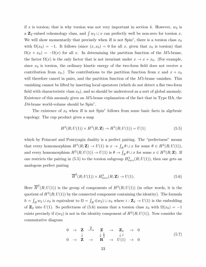
if x is torsion; that is why torsion was not very important in section 4. However, w2 is

a Z2-valued cohomology class, and∫w2 ∪ x can perfectly well be non-zero for torsion x.

We will show momentarily that precisely when R is not Spinc, there is a torsion class x0

with Ω(x0) = −1. It follows (since (x, x0) = 0 for all x, given that x0 is torsion) that

Ω(x + x0) = −Ω(x) for all x. In determining the partition function of the M5-brane,

the factor Ω(x) is the only factor that is not invariant under x → x + x0. (For example,

since x0 is torsion, the ordinary kinetic energy of the two-form field does not receive a

contribution from x0.) The contributions to the partition function from x and x + x0

will therefore cancel in pairs, and the partition function of the M5-brane vanishes. This

vanishing cannot be lifted by inserting local operators (which do not detect a flat two-form

field with characteristic class x0), and so should be understood as a sort of global anomaly.

Existence of this anomaly gives an M5-brane explanation of the fact that in Type IIA, the

D4-brane world-volume should be Spinc.

The existence of x0 when R is not Spinc follows from some basic facts in algebraic

topology. The cup product gives a map

H2(R;U(1))×H3(R;Z) → H5(R;U(1)) = U(1) (5.5)

which by Poincare and Pontryagin duality is a perfect pairing. The “perfectness” means

that every homomorphism H3(R;Z) → U(1) is x →∫Rθ ∪ x for some θ ∈ H2(R;U(1)),

and every homomorphism H2(R;U(1)) → U(1) is θ →∫Rθ ∪ x for some x ∈ H3(R;Z). If

one restricts the pairing in (5.5) to the torsion subgroup H3tors(R;U(1)), then one gets an

analogous perfect pairing

H2(R;U(1))×H3

tors(R;Z) → U(1). (5.6)

Here H2(R;U(1)) is the group of components of H2(R;U(1)) (in other words, it is the

quotient ofH2(R;U(1)) by the connected component containing the identity). The formula

h =∫Rw2 ∪ x0 is equivalent to Ω =

∫Ri(w2) ∪ x0 where i : Z2 → U(1) is the embedding

of Z2 into U(1). So perfectness of (5.6) means that a torsion class x0 with Ω(x0) = −1

exists precisely if i(w2) is not in the identity component of H2(R;U(1)). Now consider the

commutative diagram

0 → Z2−→ Z → Z2 → 0

↓ ↓ 12

↓ i0 → Z → R → U(1) → 0

(5.7)

23

where the first horizontal map in the top row is multiplication by 2, the other horizontal

maps are obvious inclusions and reductions, the first vertical map is the identity, the second

vertical line is multiplication by 1/2, and the last is i. Let β : H2(R;Z2) → H3(R;Z) be

the Bockstein derived from the first row, and let β′ : H2(R;U(1)) → H3(R;Z) be the

Bockstein derived from the second. The condition that R is not Spinc is β(w2) 6= 0; in

fact, W3(R) = β(w2) is the obstruction to Spinc structure. The condition that i(w2) not

be in the identity component of H2(R;U(1)) is that β′(i(w2)) 6= 0. Commutativity of the

above diagram implies that β′ = iβ. So i(w2) is not in the identity component, and a

torsion x0 with Ω(x0) = −1 exists, if and only if W3(R) 6= 0 and R is not Spinc.

Generalizations

This discussion of a global anomaly is not limited to the case that V = S ×R. More

generally, theM5-brane is anomalous whenever there is a torsion class x0 with Ω(x0) = −1.

However, it is hard in general to give a criterion for existence of x0.

I will now briefly suggest how these anomalies can be removed by turning on back-

ground fields. In the discussion so far, we have taken the Neveu-Schwarz three-form field

H of Type IIA, and the corresponding M -theory four-form field G, to be topologically

trivial. Naively, the classical equations dT2 = H and dT = G (where T2 is the two-form on

a D4-brane and T is the self-dual three-form on an M5-brane) imply that H and G should

be trivial when restricted to the D4- and M5-brane world-volumes. However, taking into

account the global anomalies, the general statement for Type IIA is [1,4]

H|R =W3(R), (5.8)

where H|R is shorthand for the restriction to R of the characteristic class of H. The analog

of this condition for the M5-brane should apparently be the following. Under the perfect

pairing

H3(V ;U(1))×H3

tors(V ;Z) → U(1) (5.9)

analogous to the one considered above, the function x0 → Ω(x0) (for x0 torsion) corre-

sponds to an element θ ∈ H3(V ;U(1)). The general statement about the restriction of G

to V should apparently be

G|V = β′(θ), (5.10)

where as above β′ is the Bockstein. This reduces to (5.8) in the appropriate situation, and

I suspect that it holds in general.

24

5.2. Direct Computation

Let us next attempt to directly imitate the computation in section 4. To begin with,

we assume that V is spin.

For x ∈ H3(V ;Z), we want to define a suitable Z2-valued function Ω(x) = (−1)h(x).

We let Z = S′ × V (with S′ a circle) and set z = a′ ∪ x with a′ a generator of H1(S′;Z).9

Then, assuming that Z is the boundary of an eight-dimensional spin manifold W over

which z extends, one is tempted to set h(x) =∫Wz ∪ z. This is not well-defined modulo

2, because in general for a closed eight-dimensional spin manifold W ,∫Wz ∪ z is not even.

The quantity which is always even for a closed eight-dimensional spin manifold with a

given z ∈ H4(W ;Z) is∫W(z ∪ z + λ ∪ z) (where λ is the integral characteristic class with

2λ = p1(W )), so we set

h(x) =

∫

W

(z ∪ z + λ ∪ z). (5.11)

Here we need, as in the analogous discussion in section 4, to make sense of the integral∫Wλ∪z on the manifold-with-boundaryW . This integral needs some explanation, because

in general neither λ nor z vanishes on the boundary of W . The approach taken in [31]

was as follows. If (5.11) were well-defined purely topologically, we would use the function

Ω(x) to quantize the torus T = H3(V ;R)/H3(V ;Z) that parametrizes flat three-form

fields C on V mod gauge transformations. The λ ∪ z term in (5.11) means that the torus

that we can naturally quantize is not T but the torus T′ that parametrizes, up to gauge

transformations, C-fields of curvature λ/2. (T is isomorphic to T′, by the map C → C+C0

where C0 is any C-field of curvature λ/2, but there is no canonical isomorphism between

T and T′.) A heuristic way to explain the shift from T to T′ is that z → z − λ/2

eliminates the z∪λ term in (5.11); for more information, see [31]. An alternative approach

to understanding the integral in (5.11) (described to me by M. Hopkins and I. M. Singer)

9 The following computation has a very similar structure to the one in section 4, although a few

details are different. To try to bring out the analogy, and hopefully without causing confusion, we

will use some of the notation of section 4 for objects that play the analogous role here. The seven-

manifold Z is analogous to the eleven-manifold called Z in section 4; likewise, the eight-manifold

W of boundary Z will be analogous to the twelve-manifold called W in section 4. Similarly, we

will use the names S′, a′, x, and z for objects that play an analogous role to objects of the same

name in section 4.

25

is as follows. The λ class of a seven-dimensional spin manifold such as Z is always even.10

Since we only want to define h(x) modulo 2, we can interpret the integral∫Wλ ∪ z as an

integral in mod 2 cohomology, replacing λ and z by their mod 2 reductions λ and z. Since

λ vanishes when restricted to the boundary of W , we can pick a trivialization of it; once

such a trivialization is picked, the integral∫Wλ∪ z makes sense. The relation between the

two approaches is that a trivialization of λ mod 2 gives a way of identifying T and T′.

The details in the last paragraph will not play a major role in the present paper. The

reason is that, with V = S ×R, we will compute Ω(x) only for x ∈ H3(R;Z). This means

that on Z = S′ × V = S′ × S × R, both λ and z = a′ ∪ x are pullbacks from S′ × R. In

trivializing λ mod 2 on Z, we can restrict ourselves to consider only trivializations that

are pulled back from R, and the choice of such a trivialization does not affect the integral∫Wλ∪z. At the level of differential forms, this last statement means that under λ→ λ+dγ,

∫Wλ ∪ z changes by

∫S′×S×R

γ ∪ z, which vanishes for γ and z both being pullbacks from

S′ ×R. Hence there is a completely canonical Ω(x) for the x we will consider, and this is

what we will evaluate.

Just as in section 4.2, it is inconvenient to calculate with W required to be a spin

manifold. We can readily generalize the discussion to permit V and W to be Spinc mani-

folds, not necessarily spin, as follows. A Spinc manifold W (with a chosen Spinc structure)

has a two-dimensional class α ∈ H2(W ;Z), which reduces mod 2 to w2(W ). In addition,

on such a manifold p1 − α2 is divisible by 2, and there is an integral characteristic class λ

such that11 2λ = p1 − α2. Moreover, for any x ∈ H4(W ;Z),∫W(x ∪ x+ λ ∪ x) is always

even.12 So we can evaluate (5.11) for any Spinc manifold W , with λ as just defined.

10 The intersection form of the eight-manifold B = S1× V is even, so the relation

∫B(x ∪ x+

λ∪x) ∼= 0 modulo 2 for all x ∈ H4(B;Z) reduces to∫Bλ∪x ∼= 0 modulo 2 for all x. This implies

that λ is divisible by 2.11 More generally, any real oriented vector bundle E with w2(E) = 0 has an integral character-

istic class λ with 2λ(E) = p1(E). If W is Spinc, let J be a real two-plane bundle with Euler class

α, and let E = TW ⊕ J (with TW being the tangent bundle to W ). Then w2(E) = 0, and λ(E)

is the desired class with 2λ = p1(E) = p1(TW )− α2.12 This can be proved by generalizing the proof given in section 4 of [5] (see eqn. (4.7)), where

W was assumed to be spin. Let J be a real two-plane bundle over W with Euler class α, and let

N be the direct sum of J with a trivial rank three bundle. Let K be a twelve-manifold that is

the unit sphere bundle in N ; K is spin. Let π : K → W be the projection, let x be any element

of H4(W ;Z), and let u be an element of H4(K;Z) with π∗(u) = 1 and u ∪ u = 0. (Such a u can

be constructed as the Poincare dual of a section of π.) Consider, as in [5], an E8 bundle B over

26

We will now consider h(x) for V = S × R. We assume first that R is Spinc. We

give V a Spinc structure that is the product of the supersymmetric (or unbounding) spin

structure on S with the given Spinc structure on R. We set Z = S′ × V = S′ × S × R.

Suppose that x ∈ H3(R;Z). Then as in section 4.2, Z is the boundary of a Spinc manifold

W = S′ ×D × R, where D is a disc of boundary S; and z = a′ ∪ x extends over W as a

pullback from S′ ×R. The Spinc structure on W is the product of a spin structure on S′,

the given Spinc structure on R with two-dimensional class αR, and a Spinc structure on D

with a two-dimensional class αD such that∫DαD = 1. (The reason for the last statement

is the same as in section 4.2: the supersymmetric spin structure on S does not extend

over D as a spin structure, but it extends as a Spinc structure with∫DαD = 1.) We have

p1(W ) = p1(R) and α(W ) = αD + αR; also, αD ∪αD = 0 since D is two-dimensional. We

can compute the λ class of W : λ(W ) = (p1(W )−α(W )2)/2 = λ(R)−αD ∪αR. It follows

that

h(x) =

∫

W

(z ∪ z + λ(w) ∪ z) =∫

W

(z ∪ z + λ(R) ∪ z − αD ∪ αR ∪ z) . (5.12)

On the right hand side, only the term αD∪αR∪z contributes to the integral, as the others

are pullbacks from S′ ×R. Using z = a′ ∪ x, with∫S′a′ = 1, and

∫DαD = 1, we get

h(x) = −∫

R

αR ∪ x. (5.13)

Since αR is congruent to w2(R) mod 2, this is equivalent to the promised formula (5.2).

So far we have assumed that V is Spinc. Otherwise, the λ class is no longer available,

but we still have the Wu class v in mod 2 cohomology, with∫W(x ∪ x + v ∪ x) even. In

eight dimensions,

v = w22 + w4. (5.14)

So the definition of h(x) should be

h(x) =

∫

W

(z ∪ z + (w4 + w2

2) ∪ z). (5.15)

K with characteristic class u+ π∗(x). If i(B) is the index of the Dirac operator on K with values

in B (in the adjoint representation), then i(B) is even (because B is real and K has dimension

of the form 8k + 4). Evaluation of i(B) via the index theorem leads, as in [5] (and using the fact

that λ(K) = π∗(λ(W )) where λ(W ) is defined as in the last footnote using the Spinc structure of

W ), to i(B) =∫W(x ∪ x+ λ(W ) ∪ x), and so this expression is even.

27

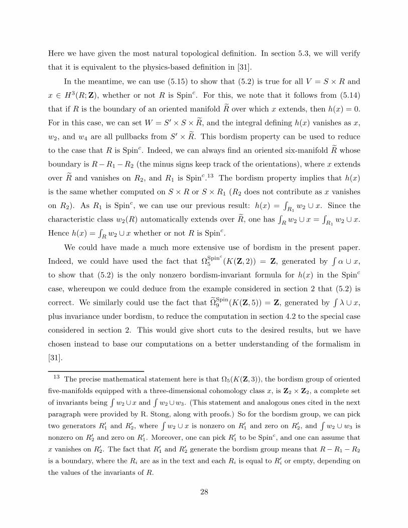
Here we have given the most natural topological definition. In section 5.3, we will verify

that it is equivalent to the physics-based definition in [31].

In the meantime, we can use (5.15) to show that (5.2) is true for all V = S × R and

x ∈ H3(R;Z), whether or not R is Spinc. For this, we note that it follows from (5.14)

that if R is the boundary of an oriented manifold R over which x extends, then h(x) = 0.

For in this case, we can set W = S′ × S × R, and the integral defining h(x) vanishes as x,

w2, and w4 are all pullbacks from S′ × R. This bordism property can be used to reduce

to the case that R is Spinc. Indeed, we can always find an oriented six-manifold R whose

boundary is R−R1−R2 (the minus signs keep track of the orientations), where x extends

over R and vanishes on R2, and R1 is Spinc.13 The bordism property implies that h(x)

is the same whether computed on S ×R or S ×R1 (R2 does not contribute as x vanishes

on R2). As R1 is Spinc, we can use our previous result: h(x) =∫R1

w2 ∪ x. Since the

characteristic class w2(R) automatically extends over R, one has∫Rw2 ∪ x =

∫R1

w2 ∪ x.Hence h(x) =

∫Rw2 ∪ x whether or not R is Spinc.

We could have made a much more extensive use of bordism in the present paper.

Indeed, we could have used the fact that ΩSpinc

5 (K(Z, 2)) = Z, generated by∫α ∪ x,

to show that (5.2) is the only nonzero bordism-invariant formula for h(x) in the Spinc

case, whereupon we could deduce from the example considered in section 2 that (5.2) is

correct. We similarly could use the fact that ΩSpin9 (K(Z, 5)) = Z, generated by

∫λ ∪ x,

plus invariance under bordism, to reduce the computation in section 4.2 to the special case

considered in section 2. This would give short cuts to the desired results, but we have

chosen instead to base our computations on a better understanding of the formalism in

[31].

13 The precise mathematical statement here is that Ω5(K(Z, 3)), the bordism group of oriented

five-manifolds equipped with a three-dimensional cohomology class x, is Z2 × Z2, a complete set

of invariants being∫w2 ∪x and

∫w2 ∪w3. (This statement and analogous ones cited in the next

paragraph were provided by R. Stong, along with proofs.) So for the bordism group, we can pick

two generators R′

1 and R′

2, where∫w2 ∪ x is nonzero on R′

1 and zero on R′

2, and∫w2 ∪ w3 is

nonzero on R′

2 and zero on R′

1. Moreover, one can pick R′

1 to be Spinc, and one can assume that

x vanishes on R′

2. The fact that R′

1 and R′

2 generate the bordism group means that R−R1 −R2

is a boundary, where the Ri are as in the text and each Ri is equal to R′

i or empty, depending on

the values of the invariants of R.

28

5.3. Comparison To Physical Definition

It remains to compare the obvious topological definition (5.15) to the physics-based

formalism in [31]. The full physical setup for this problem depends on details that we have

so far omitted. The M5-brane worldvolume V is embedded in an eleven-manifold M . V

is orientable (but not necessarily spin), and M is spin. Let N be the normal bundle to V

in M . The condition for M to be spin is

w1(N) = 0, w2(N) = w2(V ). (5.16)

Also, the Euler class of N vanishes (or equivalently, as N is of odd rank, w5(N) = 0), for

reasons explained in section 5 of [5]. Another part of the data is the four-form field G of

M -theory. It is of the formG

2π=λ(M)

2+ g, (5.17)

where g is an integral class. Moreover, if U is a small four-sphere linking V in M , then

∫

U

g = 1, (5.18)

since the fivebrane has unit charge.

Let P be the submanifold of M consisting of all points a distance ǫ from V , for some

very small ǫ. P is a four-sphere bundle over V . Let π : P → V be the projection. (5.18)

is the statement that

π∗(g) = 1. (5.19)

This uniquely determines g modulo g → g + π∗(y) for y ∈ H4(V ;Z). Note that π∗(g ∪ g)is invariant mod 2 under such a transformation of g. Hence, its mod 2 reduction does not

depend on the choice of g. In fact,

π∗(g ∪ g) ∼= w4(N) mod 2. (5.20)

To prove this, since the left hand side is independent of the choice of g modulo 2, it suffices

to consider the case that g is the Poincare dual to a section s of π. (Such a section exists

at least over the five-skeleton of V , since the Euler class of N is zero, and a choice of s on

the five-skeleton suffices for evaluating the four-dimensional class on the left hand side of

(5.20).) Choice of such a section splits N as N = O⊕N ′ where O is a rank one trivial real

bundle (consisting of multiples of s) and N ′ is a rank four bundle. g ∪ g is Poincare dual

29

to the intersection class s∩ s. If we regard s as a codimension four submanifold of P , then

its normal bundle is N ′, so s∩s is dual to the restriction to s of the Euler class χ(N ′), and

hence π∗(g∪ g) = π∗(g∪χ(N ′)) = π∗(g)∪χ(N ′) = χ(N ′). But (for any SO(4) bundle N ′)

χ(N ′) is congruent to w4(N′) mod 2, and with N = O ⊕ N ′, we have w4(N) = w4(N

′).

This justifies the assertion in (5.20).

Pick a class x ∈ H3(V ;Z). We will now restate the definition of Ω(x) = (−1)h(x) given

in [31]. Let z = a′ ∪ x ∈ H4(S′ × V ;Z), with a′ a generator of H1(S′;Z). Let Z = S′ ×P ,

where S′ is a circle with Neveu-Schwarz spin structure. Thus, Z is a four-sphere bundle

over Z = S′ × V ; we write π for the projection π : Z → Z. And define w ∈ H4(Z;Z) by

w = π∗(z) + g. Let now W be a twelve-dimensional spin manifold with boundary Z over

which w extends. Such a W always exists [40]. The definition in [31] can be stated

h(x) =1

3

∫

W

(w − 1

2λ

)((w − 1

2λ)2 − 1

8(p2 − λ2)

)− (w → 0) . (5.21)

Here the meaning of the last term is that one should subtract the same expression with

w replaced by 0. E8 index theory is used to prove that h(x) is integral and independent

modulo 2 of the choice of W and of the extension of w. The fact that the class that is

integrated in (5.21) is not canonically trivial near the boundary means that the function

Ω(x) enables us to quantize not the space H3(V ;U(1)) of flat three-form fields on V , but

a shifted version of it.

The definition of h(x) just given is rather abstract. For computation, it is convenient

to make some simplifying assumptions that are actually rather mild in practice. Suppose

that S′ × V is the boundary of an oriented eight-manifold W over which N extends (as a

rank five bundle obeying w1(N) = 0, w2(N) = w2(W ), and w5(N) = 0). Let W be the

unit sphere bundle in N ; the conditions on N ensure that W is spin, and its boundary is

Z = S′ × P . Suppose further that z = a′ ∪ x extends over W , and that g extends over

W . Then, setting w = π∗(z) + g, we can simplify (5.21) by integrating over the fibers of

π : W →W . We get

h(x) =

∫

W

(z ∪ z − z ∪ λ(W ) + z ∪ π∗(g ∪ g)

). (5.22)

(We have dropped terms that vanish if x = 0; they in fact vanish mod 2 using the fact that

the integral in (5.21) is even if evaluated on a closed twelve-dimensional spin manifold,

and the fact that the integrand vanishes near the boundary if x = 0.)

30

To clarify this further, we would like to express the mod 2 reduction of −λ(W ) +

π∗(g∪g) in terms of quantities defined just on W . For this, we note first that (for any spin

manifold W ) λ(W ) is congruent mod 2 to w4(W ). Stably, the tangent bundles TW and TW

of W and W are related by TW = TW ⊕N . So since w1(W ) = w1(N) = 0 and w2(N) =

w2(W ), we have w4(W ) = w4(W ) +w2(W )w2(N) +w4(N) = w4(W ) +w2(W )2 +w4(N).

Using also (5.20), we learn that −λ(W )+π∗(g∪g) is congruent mod 2 to w4(W )+w2(W )2,

so that (5.22) is equivalent to

h(x) =

∫

W

(z ∪ z + w4(W ) ∪ z + w2(W ) ∪ w2(W ) ∪ z) . (5.23)

This is the formula that we guessed on purely formal grounds toward the end of section

5.2. What we have gained is an understanding of how this formula is related to eleven-

dimensional physics.

This work was supported in part by NSF Grant PHY-9513835 and the Caltech Dis-

covery Fund. I am grateful to M. J. Hopkins and I. M. Singer for numerous explanations of

their viewpoint about the fivebrane action, as well as other matters. In addition, I would

like to thank G. Moore for discussions and suggestions about the manuscript, R. Stong for

helpful correspondence, and E. Diaconescu, D. Freed, and A. Kapustin for comments and

questions.

31

References

[1] E. Witten, “Baryons and Branes In Anti de Sitter Space,” JHEP 9807:006 (1998),

hep-th/9805112.

[2] R. Minasian and G. Moore, “K Theory And Ramond-Ramond Charge,” JHEP

9711:002 (1997), hep-th/9710230.

[3] E. Witten, “D-Branes And K Theory,” JHEP 9812:019 (1998), hep-th/9810188.

[4] D. Freed and E. Witten, “Anomalies In String Theory With D-Branes,” hep-

th/9907189.

[5] E. Witten, “On Flux Quantization InM Theory And The Effective Action,” J. Geom.

Phys. 22 (1997) 1, hep-th/9609122.

[6] N. Marcus and J. H. Schwarz, “Field Theories That Have No Manifestly Lorentz

Invariant Formulation,” Phys. Lett. B115 (1982) 111.

[7] W. Siegel, “Manifest Lorentz Invariance Sometimes Requires Nonlinearity,” Nucl.

Phys. B238 (184) 307.

[8] P. Goddard and D. Olive, “Algebras, Lattices, and Strings” (preprint, 1983), Phys.

Scripta T15 (1987).

[9] C. Imbimbo and A. Schwimmer, “The Lagrangian Formulation Of Chiral Scalars,”

Phys. Lett. B193 (1987) 455.

[10] C. M. Hull, “Covariant Quantization Of Chiral Bosons And Anomaly Cancellation,”

Phys. Lett. B206 (1988) 234.

[11] J. M. F. Labastida and M. Pernici, “Lagrangians For Chiral Bosons And The Heterotic

String,” Nucl. Phys. B306 (1988) 516.

[12] L. Mezincescu and R. I. Nepomechie, “Critical Dimensions For Chiral Bosons,” Phys.

Rev. D37 (1988) 3067.

[13] M. Henneaux and C. Teitelboim, “Dynamics Of Chiral (Selfdual) p Forms,” Phys.

Lett. B206 (1988) 650; F. P. Devecchi and M. Henneaux, “Covariant Path Integral

For Chiral p-Forms,” Phys. Rev. D54 (1996) 1606.

[14] P. P. Srivastava, “On A Gauge Theory Of Selfdual Field And Its Quantization,” Phys.

Lett. B234 (1990) 93.

[15] B. McClain, Y. S. Wu, and F. Yu, “Covariant Quantization Of Chiral Bosons and

OSp(1, 1|2) Symmetry, Nucl. Phys. B343 (1990) 689.

[16] C. Wotzase, “The Wess-Zumino Term For Chiral Bosons,” Phys. Rev. Lett. 66 (1991)

129.

[17] I. Martin and A. Restuccia, “Duality Symmetric Actions And Canonical Quantiza-

tion,” Phys. Lett. B323 (1994) 311.

[18] J. H. Schwarz and A. Sen, “Duality Symmetric Actions,” Nucl. Phys. B411 (1994)

35, hep-th/9304154.

32

[19] E. Verlinde, “Global Aspects Of Electric-Magnetic Duality,” Nucl. Phys. B455 (1995)

211, hep-th/9506011.

[20] M. Perry and J. H. Schwarz, “Interacting Chiral Gauge Fields In Six Dimensional

Born-Infeld Theory,” hep-th/9611065.

[21] J. H. Schwarz, “Coupling A Self-Dual Tensor To Gravity In Six Dimensions,” hep-

th/9701008.

[22] N. Berkovits, “Local Actions With Electric and Magnetic Sources,” hep-th/9610134,

“Super-Maxwell Actions With Manifest Duality,” hep-th/9612174.

[23] I. Bengtsson and A. Kleppe, “On Chiral p-Forms,” hep-th/9609102; I. Bengtsson,

“Manifest Duality In Born-Infeld Theory,” hep-th/9612174.

[24] P. Pasti, D. Sorokin, and M. Tonin, Phys. Lett. B352 (1995) 59, Phys. Rev. D52

(1995) R4277, “On Lorentz Invariant Actions For Chiral P -Forms,” hep-th/9611100,

“Covariant Action For A D = 11 Five-Brane With The Chiral Field,” Phys. Lett.

B398 (1997) 41; I. Bandos, K. Lechner, A. Nurmagambetov, P. Pasti, D. Sorokin,

“Covariant Action For The Super-Five-Brane Of M -Theory,” hep-th/9701149; G.

Dall’Agata, K. Lechner, and M. Tonin, “Action For IIB SUpergravity In Ten Di-

mensions,” hep-th/9812170.

[25] M. Aganagic, J. Park, C. Popescu, and J. Schwarz, “Worldvolume Action For The

M -Theory Fivebrane,” Nucl. Phys. B496 (1997) 191, hep-th/9701166.

[26] P. S. Howe, E. Sezgin, and P. C. West, “Covariant Field Equations Of The M Theory

Five-Brane,” Phys. Lett.B399 (1997) 49, hep-th/9702008, “The Six-Dimensional Self-

Dual Tensor,” Phys. Lett. B400 (1997) 255, hep-th/9702111.

[27] Y.-G. Miao, J.-G. Zhou, and Y.-Y. Liu, “New Way Of The Derivation Of First Order

Wess-Zumino Terms,” Phys. Lett. B323 (1994) 169; Y.-G. Miao and H. J. W. Muller-

Kirsten, “Self-Duality Of Various Chiral Boson Actions,” hep-th/9912066.

[28] A. Mazyntsia, C. R. Preitschopf, and D. Sorokin, “Dual Actions For Chiral Bosons,”

hep-th/9808049.

[29] X. Bekaert, M. Henneaux, and A. Sevrin, “Deformations Of Chiral Two-Forms In

Six Dimensions,” hep-th/9909094, “Symmetry-deforming Interactions Of Chiral p-

Forms,” hep-th/9912077.

[30] M. Henningson, B. E. W. Nilsson, and P. Salomonson, “Holomorphic Factorization

Of Correlation Functions In (4k + 2)-Dimensional (2k)-Form Gauge Theory,” hep-

th/9908107.

[31] E. Witten, “Fivebrane Effective Action In M -Theory,” J. Geom. Phys. 22 (1997) 103,

hep-th/9610234.

[32] L. Dolan and C. R. Nappi, “A Modular Invariant Partition Function For The Five-

Brane,” Nucl. Phys. B530 (1998) 683, hep-th/9806016.

[33] M. Hopkins and I. M. Singer, to appear.

33

[34] D. J. Gross, J. A. Harvey, E. Martinec, and R. Rohm, “The Heterotic String,” Phys.

Rev. Lett. 54 (1985) 502.

[35] D. Freed, J. A. Harvey, R. Minasian, and G. Moore, “Gravitational Anomaly Can-

cellation For M Theory Five-Branes,” Adv. Theor. Math. Phys. 2 (1998) 601, hep-

th/9803205.

[36] K. Becker and M. Becker, “Five-Brane Gravitational Anomalies,” hep-th/9911138.

[37] E. Witten, “On S Duality In Abelian Gauge Theory,” hep-th/9505186.

[38] M. F. Atiyah and I. M. Singer, “The Index Of Elliptic Operators: V,” Ann. Math. 93

(1971) 139.

[39] M. F. Atiyah, “K-Theory And Reality,” Quart. J. Math., Oxford (2) 17 (1966) 367.

[40] R. Stong, “Calculation Of Ωspin11 (K(Z, 4),” in Unified String Theories, eds. M. B. Green

and D. J. Gross (World Scientific, 1986).

34