arX

iv:h

ep-t

h/99

0814

2v3

30

Nov

199

9

IASSNS-HEP-99/74

hep-th/9908142

String Theory and Noncommutative Geometry

Nathan Seiberg and Edward Witten

School of Natural Sciences

Institute for Advanced Study

Olden Lane, Princeton, NJ 08540

We extend earlier ideas about the appearance of noncommutative geometry in string theory

with a nonzero B-field. We identify a limit in which the entire string dynamics is described

by a minimally coupled (supersymmetric) gauge theory on a noncommutative space, and

discuss the corrections away from this limit. Our analysis leads us to an equivalence

between ordinary gauge fields and noncommutative gauge fields, which is realized by a

change of variables that can be described explicitly. This change of variables is checked by

comparing the ordinary Dirac-Born-Infeld theory with its noncommutative counterpart.

We obtain a new perspective on noncommutative gauge theory on a torus, its T -duality,

and Morita equivalence. We also discuss the D0/D4 system, the relation to M -theory in

DLCQ, and a possible noncommutative version of the six-dimensional (2, 0) theory.

8/99

1. Introduction

The idea that the spacetime coordinates do not commute is quite old [1]. It has been

studied by many authors both from a mathematical and a physical perspective. The theory

of operator algebras has been suggested as a framework for physics in noncommutative

spacetime – see [2] for an exposition of the philosophy – and Yang-Mills theory on a

noncommutative torus has been proposed as an example [3]. Though this example at first

sight appears to be neither covariant nor causal, it has proved to arise in string theory in a

definite limit [4], with the noncovariance arising from the expectation value of a background

field. This analysis involved toroidal compactification, in the limit of small volume, with

fixed and generic values of the worldsheet theta angles. This limit is fairly natural in the

context of the matrix model of M -theory [5,6], and the original discussion was made in

this context. Indeed, early work relating membranes to large matrices [7], has motivated

in [8,9] constructions somewhat similar to [3]. For other thoughts about applications of

noncommutative geometry in physics, see e.g. [10]. Noncommutative geometry has also

been used as a framework for open string field theory [11].

Part of the beauty of the analysis in [4] was that T -duality acts within the non-

commutative Yang-Mills framework, rather than, as one might expect, mixing the modes

of noncommutative Yang-Mills theory with string winding states and other stringy ex-

citations. This makes the framework of noncommutative Yang-Mills theory seem very

powerful.

Subsequent work has gone in several directions. Additional arguments have been

presented extracting noncommutative Yang-Mills theory more directly from open strings

without recourse to matrix theory [12-16]. The role of Morita equivalence in establishing

T -duality has been understood more fully [17,18]. The modules and their T -dualities have

been reconsidered in a more elementary language [19-21], and the relation to the Dirac-

Born-Infeld Lagrangian has been explored [20,21]. The BPS spectrum has been more

fully understood [19,20,22]. Various related aspects of noncommutative gauge theories

have been discussed in [23-32]. Finally, the authors of [33] suggested interesting relations

between noncommutative gauge theory and the little string theory [34].

Large Instantons And The α′ Expansion

Our work has been particularly influenced by certain further developments, including

the analysis of instantons on a noncommutative R4 [35]. It was shown that instantons on

a noncommutative R4 can be described by adding a constant (a Fayet-Iliopoulos term)

1

to the ADHM equations. This constant had been argued, following [36], to arise in the

description of instantons on D-branes upon turning on a constant B-field [37], 1 so putting

the two facts together it was proposed that instantons on branes with a B-field should be

described by noncommutative Yang-Mills theory [35,38].

Another very cogent argument for this is as follows. ConsiderN parallel threebranes of

Type IIB. They can support supersymmetric configurations in the form of U(N) instantons.

If the instantons are large, they can be described by the classical self-dual Yang-Mills

equations. If the instantons are small, the classical description of the instantons is no

longer good. However, it can be shown that, at B = 0, the instanton moduli space M in

string theory coincides precisely with the classical instanton moduli space. The argument

for this is presented in section 2.3. In particular, M has the small instanton singularities

that are familiar from classical Yang-Mills theory. The significance of these singularities

in string theory is well known: they arise because an instanton can shrink to a point and

escape as a −1-brane [39,40]. Now if one turns on a B-field, the argument that the stringy

instanton moduli space coincides with the classical instanton moduli space fails, as we will

also see in section 2.3. Indeed, the instanton moduli space must be corrected for nonzero B.

The reason is that, at nonzero B (unless B is anti-self-dual) a configuration of a threebrane

and a separated −1-brane is not BPS,2 so an instanton on the threebrane cannot shrink

to a point and escape. The instanton moduli space must therefore be modified, for non-

zero B, to eliminate the small instanton singularity. Adding a constant to the ADHM

equations resolves the small instanton singularity [41], and since going to noncommutative

R4 does add this constant [35], this strongly encourages us to believe that instantons with

the B-field should be described as instantons on a noncommutative space.

This line of thought leads to an apparent paradox, however. Instantons come in

all sizes, and however else they can be described, big instantons can surely be described

by conventional Yang-Mills theory, with the familiar stringy α′ corrections that are of

higher dimension, but possess the standard Yang-Mills gauge invariance. The proposal in

[35] implies, however, that the large instantons would be described by classical Yang-Mills

equations with corrections coming from the noncommutativity of spacetime. For these two

1 One must recall that in the presence of a D-brane, a constant B-field cannot be gauged away

and can in fact be reinterpreted as a magnetic field on the brane.2 This is shown in a footnote in section 4.2; the configurations in question are further studied

in section 5.

2

viewpoints to agree means that noncommutative Yang-Mills theory must be equivalent to

ordinary Yang-Mills theory perturbed by higher dimension, gauge-invariant operators. To

put it differently, it must be possible (at least to all orders in a systematic asymptotic

expansion) to map noncommutative Yang-Mills fields to ordinary Yang-Mills fields, by

a transformation that maps one kind of gauge invariance to the other and adds higher

dimension terms to the equations of motion. This at first sight seems implausible, but we

will see in section 3 that it is true.

Applying noncommutative Yang-Mills theory to instantons on R4 leads to another

puzzle. The original application of noncommutative Yang-Mills to string theory [4] involved

toroidal compactification in a small volume limit. The physics of noncompact R4 is the

opposite of a small volume limit! The small volume limit is also puzzling even in the case

of a torus; if the volume of the torus the strings propagate on is taken to zero, how can

we end up with a noncommutative torus of finite size, as has been proposed? Therefore, a

reappraisal of the range of usefulness of noncommutative Yang-Mills theory seems called

for. For this, it is desireable to have new ways of understanding the description of D-

brane phenomena in terms of physics on noncommuting spacetime. A suggestion in this

direction is given by recent analyses arguing for noncommutativity of string coordinates

in the presence of a B-field, in a Hamiltonian treatment [14] and also in a worldsheet

treatment that makes the computations particularly simple [15]. In the latter paper, it

was suggested that rather classical features of the propagation of strings in a constant

magnetic field [42,43] can be reinterpreted in terms of noncommutativity of spacetime.

In the present paper, we will build upon these suggestions and reexamine the quan-

tization of open strings ending on D-branes in the presence of a B-field. We will show

that noncommutative Yang-Mills theory is valid for some purposes in the presence of any

nonzero constant B-field, and that there is a systematic and efficient description of the

physics in terms of noncommutative Yang-Mills theory when B is large. The limit of a

torus of small volume with fixed theta angle (that is, fixed periods of B) [4,12] is an exam-

ple with large B, but it is also possible to have large B on Rn and thereby make contact

with the application of noncommutative Yang-Mills to instantons on R4. An important

element in our analysis is a distinction between two different metrics in the problem. Dis-

tances measured with respect to one metric are scaled to zero as in [4,12]. However, the

noncommutative theory is on a space with a different metric with respect to which all

distances are nonzero. This guarantees that both on Rn and on Tn we end up with a

theory with finite metric.

3

Organization Of The Paper

This paper is organized as follows. In section 2, we reexamine the behavior of open

strings in the presence of a constant B-field. We show that, if one introduces the right

variables, the B dependence of the effective action is completely described by making

spacetime noncommutative. In this description, however, there is still an α′ expansion

with all of its usual complexity. We further show that by taking B large or equivalently by

taking α′ → 0 holding the effective open string parameters fixed, one can get an effective

description of the physics in terms of noncommutative Yang-Mills theory. This analysis

makes it clear that two different descriptions, one by ordinary Yang-Mills fields and one by

noncommutative Yang-Mills fields, differ by the choice of regularization for the world-sheet

theory. This means that (as we argued in another way above) there must be a change of

variables from ordinary to noncommutative Yang-Mills fields. Once one is convinced that

it exists, it is not too hard to find this transformation explicitly: it is presented in section

3. In section 4, we make a detailed exploration of the two descriptions by ordinary and

noncommutative Yang-Mills fields, in the case of almost constant fields where one can use

the Born-Infeld action for the ordinary Yang-Mills fields. In section 5, we explore the

behavior of instantons at nonzero B by quantization of the D0-D4 system. Other aspects

of instantons are studied in sections 2.3 and 4.2. In section 6, we consider the behavior of

noncommutative Yang-Mills theory on a torus and analyze the action of T -duality, showing

how the standard action of T -duality on the underlying closed string parameters induces

the action of T -duality on the noncommutative Yang-Mills theory that has been described

in the literature [17-21]. We also show that many mathematical statements about modules

over a noncommutative torus and their Morita equivalences – used in analyzing T -duality

mathematically – can be systematically derived by quantization of open strings. In the

remainder of the paper, we reexamine the relation of noncommutative Yang-Mills theory

to DLCQ quantization of M -theory, and we explore the possible noncommutative version

of the (2, 0) theory in six dimensions.

Conventions

We conclude this introduction with a statement of our main conventions about non-

commutative gauge theory.

For Rn with coordinates xi whose commutators are c-numbers, we write

[xi, xj] = iθij (1.1)

4

with real θ. Given such a Lie algebra, one seeks to deform the algebra of functions on Rn

to a noncommutative, associative algebra A such that f ∗ g = fg + 12iθij∂if∂jg + O(θ2),

with the coefficient of each power of θ being a local differential expression bilinear in f and

g. The essentially unique solution of this problem (modulo redefinitions of f and g that

are local order by order in θ) is given by the explicit formula

f(x) ∗ g(x) = ei2 θij ∂

∂ξi∂

∂ζj f(x+ ξ)g(x+ ζ)∣∣ξ=ζ=0

= fg +i

2θij∂if∂jg + O(θ2). (1.2)

This formula defines what is often called the Moyal bracket of functions; it has appeared

in the physics literature in many contexts, including applications to old and new matrix

theories [8,9,44-46]. We also consider the case of N ×N matrix-valued functions f, g. In

this case, we define the ∗ product to be the tensor product of matrix multiplication with

the ∗ product of functions as just defined. The extended ∗ product is still associative.

The ∗ product is compatible with integration in the sense that for functions f , g that

vanish rapidly enough at infinity, so that one can integrate by parts in evaluating the

following integrals, one has ∫Tr f ∗ g =

∫Tr g ∗ f. (1.3)

Here Tr is the ordinary trace of the N ×N matrices, and∫

is the ordinary integration of

functions.

For ordinary Yang-Mills theory, we write the gauge transformations and field strength

asδλAi = ∂iλ+ i[λ,Ai]

Fij = ∂iAj − ∂jAi − i[Ai, Aj]

δλFij = i[λ, Fij ],

(1.4)

where A and λ are N ×N hermitian matrices. The Wilson line is

W (a, b) = Pei∫

a

bA, (1.5)

where in the path ordering A(b) is to the right. Under the gauge transformation (1.4)

δW (a, b) = iλ(a)W (a, b)− iW (a, b)λ(b). (1.6)

For noncommutative gauge theory, one uses the same formulas for the gauge transfor-

mation law and the field strength, except that matrix multiplication is replaced by the ∗product. Thus, the gauge parameter λ takes values in A tensored with N ×N hermitian

5

matrices, for some N , and the same is true for the components Ai of the gauge field A.

The gauge transformations and field strength of noncommutative Yang-Mills theory are

thusδλAi = ∂iλ+ iλ ∗ Ai − iAi ∗ λ

Fij = ∂iAj − ∂jAi − iAi ∗ Aj + iAj ∗ Ai

δλFij = iλ ∗ Fij − iFij ∗ λ.

(1.7)

The theory obtained this way reduces to conventional U(N) Yang-Mills theory for θ → 0.

Because of the way that the theory is constructed from associative algebras, there seems

to be no convenient way to get other gauge groups. The commutator of two infinitesimal

gauge transformations with generators λ1 and λ2 is, rather as in ordinary Yang-Mills

theory, a gauge transformation generated by i(λ1 ∗ λ2 − λ2 ∗ λ1). Such commutators are

nontrivial even for the rank 1 case, that is N = 1, though for θ = 0 the rank 1 case is

the Abelian U(1) gauge theory. For rank 1, to first order in θ, the above formulas for the

gauge transformations and field strength read

δλAi = ∂iλ− θkl∂kλ∂lAi + O(θ2)

Fij = ∂iAj − ∂jAi + θkl∂kAi∂lAj + O(θ2)

δλFij = −θkl∂kλ∂lFij + O(θ2).

(1.8)

Finally, a matter of terminology: we will consider the opposite of a “noncommutative”

Yang-Mills field to be an “ordinary” Yang-Mills field, rather than a “commutative” one.

To speak of ordinary Yang-Mills fields, which can have a nonabelian gauge group, as being

“commutative” would be a likely cause of confusion.

2. Open Strings In The Presence Of Constant B-Field

2.1. Bosonic Strings

In this section, we will study strings in flat space, with metric gij , in the presence

of a constant Neveu-Schwarz B-field and with Dp-branes. The B-field is equivalent to a

constant magnetic field on the brane; the subject has a long history and the basic formulas

with which we will begin were obtained in the mid-80’s [42,43].

We will denote the rank of the matrix Bij as r; r is of course even. Since the compo-

nents of B not along the brane can be gauged away, we can assume that r ≤ p+ 1. When

our target space has Lorentzian signature, we will assume that B0i = 0, with “0” the time

6

direction. With a Euclidean target space we will not impose such a restriction. Our dis-

cussion applies equally well if space is R10 or if some directions are toroidally compactified

with xi ∼ xi +2πri. (One could pick a coordinate system with gij = δij , in which case the

identification of the compactified coordinates may not be simply xi ∼ xi + 2πri, but we

will not do that.) If our space is R10, we can pick coordinates so that Bij is nonzero only

for i, j = 1, . . . , r and that gij vanishes for i = 1, . . . , r, j 6= 1, . . . , r. If some of the coordi-

nates are on a torus, we cannot pick such coordinates without affecting the identification

xi ∼ xi +2πri. For simplicity, we will still consider the case Bij 6= 0 only for i, j = 1, . . . , r

and gij = 0 for i = 1, . . . , r, j 6= 1, . . . , r.

The worldsheet action is

S =1

4πα′

∫

Σ

(gij∂ax

i∂axj − 2πiα′Bijǫab∂ax

i∂bxj)

=1

4πα′

∫

Σ

gij∂axi∂axj − i

2

∫

∂Σ

Bijxi∂tx

j ,

(2.1)

where Σ is the string worldsheet, which we take to be with Euclidean signature. (With

Lorentz signature, one would omit the “i” multiplying B.) ∂t is a tangential derivative

along the worldsheet boundary ∂Σ. The equations of motion determine the boundary

conditions. For i along the Dp-branes they are

gij∂nxj + 2πiα′Bij∂tx

j∣∣∂Σ

= 0, (2.2)

where ∂n is a normal derivative to ∂Σ. (These boundary conditions are not compatible with

real x, though with a Lorentzian worldsheet the analogous boundary conditions would be

real. Nonetheless, the open string theory can be analyzed by determining the propagator

and computing the correlation functions with these boundary conditions. In fact, another

approach to the open string problem is to omit or not specify the boundary term with B

in the action (2.1) and simply impose the boundary conditions (2.2).)

For B = 0, the boundary conditions in (2.2) are Neumann boundary conditions. When

B has rank r = p and B → ∞, or equivalently gij → 0 along the spatial directions of the

brane, the boundary conditions become Dirichlet; indeed, in this limit, the second term in

(2.2) dominates, and, with B being invertible, (2.2) reduces to ∂txj = 0. This interpolation

from Neumann to Dirichlet boundary conditions will be important, since we will eventually

take B → ∞ or gij → 0. For B very large or g very small, each boundary of the string

worldsheet is attached to a single point in the Dp-brane, as if the string is attached to

7

a zero-brane in the Dp-brane. Intuitively, these zero-branes are roughly the constituent

zero-branes of the Dp-brane as in the matrix model of M -theory [5,6], an interpretation

that is supported by the fact that in the matrix model the construction of Dp-branes

requires a nonzero B-field.

Our main focus in most of this paper will be the case that Σ is a disc, corresponding

to the classical approximation to open string theory. The disc can be conformally mapped

to the upper half plane; in this description, the boundary conditions (2.2) are

gij(∂ − ∂)xj + 2πα′Bij(∂ + ∂)xj∣∣z=z

= 0, (2.3)

where ∂ = ∂/∂z, ∂ = ∂/∂z, and Im z ≥ 0. The propagator with these boundary conditions

is [42,43]

〈xi(z)xj(z′)〉 = − α′[gij log |z − z′| − gij log |z − z′|

+Gij log |z − z′|2 +1

2πα′ θij log

z − z′

z − z′+Dij

].

(2.4)

Here

Gij =

(1

g + 2πα′B

)ij

S

=

(1

g + 2πα′Bg

1

g − 2πα′B

)ij

,

Gij = gij − (2πα′)2(Bg−1B

)ij,

θij = 2πα′(

1

g + 2πα′B

)ij

A

= −(2πα′)2(

1

g + 2πα′BB

1

g − 2πα′B

)ij

,

(2.5)

where ( )S and ( )A denote the symmetric and antisymmetric part of the matrix. The

constants Dij in (2.4) can depend on B but are independent of z and z′; they play no

essential role and can be set to a convenient value. The first three terms in (2.4) are man-

ifestly single-valued. The fourth term is single-valued, if the branch cut of the logarithm

is in the lower half plane.

In this paper, our focus will be almost entirely on the open string vertex operators

and interactions. Open string vertex operators are of course inserted on the boundary of

Σ. So to get the relevant propagator, we restrict (2.4) to real z and z′, which we denote τ

and τ ′. Evaluated at boundary points, the propagator is

〈xi(τ)xj(τ ′)〉 = −α′Gij log(τ − τ ′)2 +i

2θijǫ(τ − τ ′), (2.6)

where we have set Dij to a convenient value. ǫ(τ) is the function that is 1 or −1 for positive

or negative τ .

8

The object Gij has a very simple intuitive interpretation: it is the effective metric seen

by the open strings. The short distance behavior of the propagator between interior points

on Σ is 〈xi(z)xj(z′)〉 = −α′gij log |z − z′|. The coefficient of the logarithm determines the

anomalous dimensions of closed string vertex operators, so that it appears in the mass shell

condition for closed string states. Thus, we will refer to gij as the closed string metric.

Gij plays exactly the analogous role for open strings, since anomalous dimensions of open

string vertex operators are determined by the coefficient of log(τ − τ ′)2 in (2.6), and in

this coefficient Gij enters in exactly the way that gij would enter at θ = 0. We will refer

to Gij as the open string metric.

The coefficient θij in the propagator also has a simple intuitive interpretation, sug-

gested in [15]. In conformal field theory, one can compute commutators of operators from

the short distance behavior of operator products by interpreting time ordering as operator

ordering. Interpreting τ as time, we see that

[xi(τ), xj(τ)] = T(xi(τ)xj(τ−) − xi(τ)xj(τ+)

)= iθij . (2.7)

That is, xi are coordinates on a noncommutative space with noncommutativity parameter

θ.

Consider the product of tachyon vertex operators eip·x(τ) and eiq·x(τ ′). With τ > τ ′,

we get for the leading short distance singularity

eip·x(τ) · eiq·x(τ ′) ∼ (τ − τ ′)2α′Gijpiqje−12 iθijpiqjei(p+q)·x(τ ′) + . . . . (2.8)

If we could ignore the term (τ − τ ′)2α′p·q, then the formula for the operator product would

reduce to a ∗ product; we would get

eip·x(τ)eiq·x(τ ′) ∼ eip·x ∗ eiq·x(τ ′). (2.9)

This is no coincidence. If the dimensions of all operators were zero, the leading terms of

operator products O(τ)O′(τ ′) would be independent of τ − τ ′ for τ → τ ′, and would give

an ordinary associative product of multiplication of operators. This would have to be the

∗ product, since that product is determined by associativity, translation invariance, and

(2.7) (in the form xi ∗ xj − xj ∗ xi = iθij).

Of course, it is completely wrong in general to ignore the anomalous dimensions;

they determine the mass shell condition in string theory, and are completely essential to

the way that string theory works. Only in the limit of α′ → 0 or equivalently small

9

momenta can one ignore the anomalous dimensions. When the dimensions are nontrivial,

the leading singularities of operator products O(τ)O′(τ ′) depend on τ −τ ′ and do not give

an associative algebra in the standard sense. For precisely this reason, in formulating open

string field theory in the framework of noncommutative geometry [39], instead of using the

operator product expansion directly, it was necessary to define the associative ∗ product

by a somewhat messy procedure of gluing strings. For the same reason, most of the present

paper will be written in a limit with α′ → 0 that enables us to see the ∗ product directly

as a product of vertex operators.

B Dependence Of The Effective Action

However, there are some important general features of the theory that do not depend

on taking a zero slope limit. We will describe these first.

Consider an operator on the boundary of the disc that is of the general form

P (∂x, ∂2x, . . .)eip·x, where P is a polynomial in derivatives of x, and x are coordinates

along the Dp-brane (the transverse coordinates satisfy Dirichlet boundary conditions).

Since the second term in the propagator (2.6) is proportional to ǫ(τ − τ ′), it does not con-

tribute to contractions of derivatives of x. Therefore, the expectation value of a product

of k such operators, of momenta p1, . . . , pk, satisfies

⟨k∏

n=1

Pn(∂x(τn), ∂2x(τn), . . .)eipn·x(τn)

⟩

G,θ

= e− i

2

∑n>m

pni θijpm

j ǫ(τn−τm)

⟨k∏

n=1

Pn(∂x(τn), ∂2x(τn), . . .)eipn·x(τn)

⟩

G,θ=0

,

(2.10)

where 〈. . .〉G,θ is the expectation value with the propagator (2.6) parametrized by G and

θ. We see that when the theory is described in terms of the open string parameters G

and θ, rather than in terms of g and B, the θ dependence of correlation functions is very

simple. Note that because of momentum conservation (∑

m pm = 0), the crucial factor

exp

(− i

2

∑

n>m

pni θ

ijpmj ǫ(τn − τm)

)(2.11)

depends only on the cyclic ordering of the points τ1, . . . , τk around the circle.

The string theory S-matrix can be obtained from the conformal field theory correlators

by putting external fields on shell and integrating over the τ ’s. Therefore, it has a structure

inherited from (2.10). To be very precise, in a theory with N × N Chan-Paton factors,

10

consider a k point function of particles with Chan-Paton wave functions Wi, i = 1, . . . , k,

momenta pi, and additional labels such as polarizations or spins that we will generically

call ǫi. The contribution to the scattering amplitude in which the particles are cyclically

ordered around the disc in the order from 1 to k depends on the Chan-Paton wave functions

by a factor TrW1W2 . . .Wk. We suppose, for simplicity, that N is large enough so that

there are no identities between this factor and similar factors with other orderings. (It is

trivial to relax this assumption.) By studying the behavior of the S-matrix of massless

particles of small momenta, one can extract order by order in α′ a low energy effective

action for the theory. If Φi is an N ×N matrix-valued function in spacetime representing

a wavefunction for the ith field, then at B = 0 a general term in the effective action is a

sum of expressions of the form

∫dp+1x

√detGTr∂n1Φ1∂

n2Φ2 . . . ∂nkΦk. (2.12)

Here ∂ni is, for each i, the product of ni partial derivatives with respect to some of the

spacetime coordinates; which coordinates it is has not been specified in the notation. The

indices on fields and derivatives are contracted with the metric G, though this is not shown

explicitly in the formula.

Now to incorporate the B-field, at fixed G, is very simple: if the effective action is

written in momentum space, we need only incorporate the factor (2.11). Including this

factor is equivalent to replacing the ordinary product of fields in (2.12) by a ∗ product. (In

this formulation, one can work in coordinate space rather than momentum space.) So the

term corresponding to (2.12) in the effective action is given by the same expression but

with the wave functions multiplied using the ∗ product:

∫dp+1x

√detGTr∂n1Φ1 ∗ ∂n2Φ2 ∗ . . . ∗ ∂nkΦk. (2.13)

It follows, then, that the B dependence of the effective action for fixed G and constant B

can be obtained in the following very simple fashion: replace ordinary multiplication by

the ∗ product. We will make presently an explicit calculation of an S-matrix element to

illustrate this statement, and we will make a detailed check of a different kind in section 4

using almost constant fields and the Dirac-Born-Infeld theory.

Though we have obtained a simple description of the B-dependence of the effective

action, the discussion also makes clear that going to the noncommutative description does

not in general enable us to describe the effective action in closed form: it has an α′

11

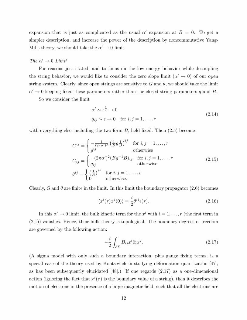
expansion that is just as complicated as the usual α′ expansion at B = 0. To get a

simpler description, and increase the power of the description by noncommutative Yang-

Mills theory, we should take the α′ → 0 limit.

The α′ → 0 Limit

For reasons just stated, and to focus on the low energy behavior while decoupling

the string behavior, we would like to consider the zero slope limit (α′ → 0) of our open

string system. Clearly, since open strings are sensitive to G and θ, we should take the limit

α′ → 0 keeping fixed these parameters rather than the closed string parameters g and B.

So we consider the limit

α′ ∼ ǫ12 → 0

gij ∼ ǫ→ 0 for i, j = 1, . . . , r(2.14)

with everything else, including the two-form B, held fixed. Then (2.5) become

Gij =

{− 1

(2πα′)2

(1B g

1B

)ijfor i, j = 1, . . . , r

gij otherwise

Gij =

{−(2πα′)2(Bg−1B)ij for i, j = 1, . . . , rgij otherwise

θij =

{(1B

)ijfor i, j = 1, . . . , r

0 otherwise.

(2.15)

Clearly, G and θ are finite in the limit. In this limit the boundary propagator (2.6) becomes

〈xi(τ)xj(0)〉 =i

2θijǫ(τ). (2.16)

In this α′ → 0 limit, the bulk kinetic term for the xi with i = 1, . . . , r (the first term in

(2.1)) vanishes. Hence, their bulk theory is topological. The boundary degrees of freedom

are governed by the following action:

− i

2

∫

∂Σ

Bijxi∂tx

j . (2.17)

(A sigma model with only such a boundary interaction, plus gauge fixing terms, is a

special case of the theory used by Kontsevich in studying deformation quantization [47],

as has been subsequently elucidated [48].) If one regards (2.17) as a one-dimensional

action (ignoring the fact that xi(τ) is the boundary value of a string), then it describes the

motion of electrons in the presence of a large magnetic field, such that all the electrons are

12

in the first Landau level. In this theory the spatial coordinates are canonically conjugate

to each other, and [xi, xj ] 6= 0. As we will discuss in section 6.3, when we construct the

representations or modules for a noncommutative torus, the fact that xi(τ) is the boundary

value of a string changes the story in a subtle way, but the general picture that the xi(τ)

are noncommuting operators remains valid.

With the propagator (2.16), normal ordered operators satisfy

: eipixi(τ) : : eiqix

i(0) := e−i2 θijpiqjǫ(τ) : eipx(τ)+iqx(0) :, (2.18)

or more generally

: f(x(τ)) : : g(x(0)) :=: ei2 ǫ(τ)θij ∂

∂xi(τ)

∂

∂xj (0) f(x(τ))g(x(0)) :, (2.19)

and

limτ→0+

: f(x(τ)) : : g(x(0)) :=: f(x(0)) ∗ g(x(0)) :, (2.20)

where

f(x) ∗ g(x) = ei2 θij ∂

∂ξi∂

∂ζj f(x+ ξ)g(x+ ζ)∣∣ξ=ζ=0

(2.21)

is the product of functions on a noncommutative space.

As always in the zero slope limit, the propagator (2.16) is not singular as τ → 0.

This lack of singularity ensures that the product of operators can be defined without a

subtraction and hence must be associative. It is similar to a product of functions, but on

a noncommutative space.

The correlation functions of exponential operators on the boundary of a disc are

⟨∏

n

eipni xi(τn)

⟩= e

− i2

∑n>m

pni θijpm

j ǫ(τn−τm)δ(∑

pn). (2.22)

Because of the δ function and the antisymmetry of θij , the correlation functions are un-

changed under cyclic permutation of τn. This means that the correlation functions are

well defined on the boundary of the disc. More generally,

⟨∏

n

fn(x(τn))

⟩=

∫dxf1(x) ∗ f2(x) ∗ . . . ∗ fn, (2.23)

which is invariant under cyclic permutations of the fn’s. As always in the zero slope limit,

the correlation functions (2.22), (2.23) do not exhibit singularities in τ , and therefore there

are no poles associated with massive string states.

13

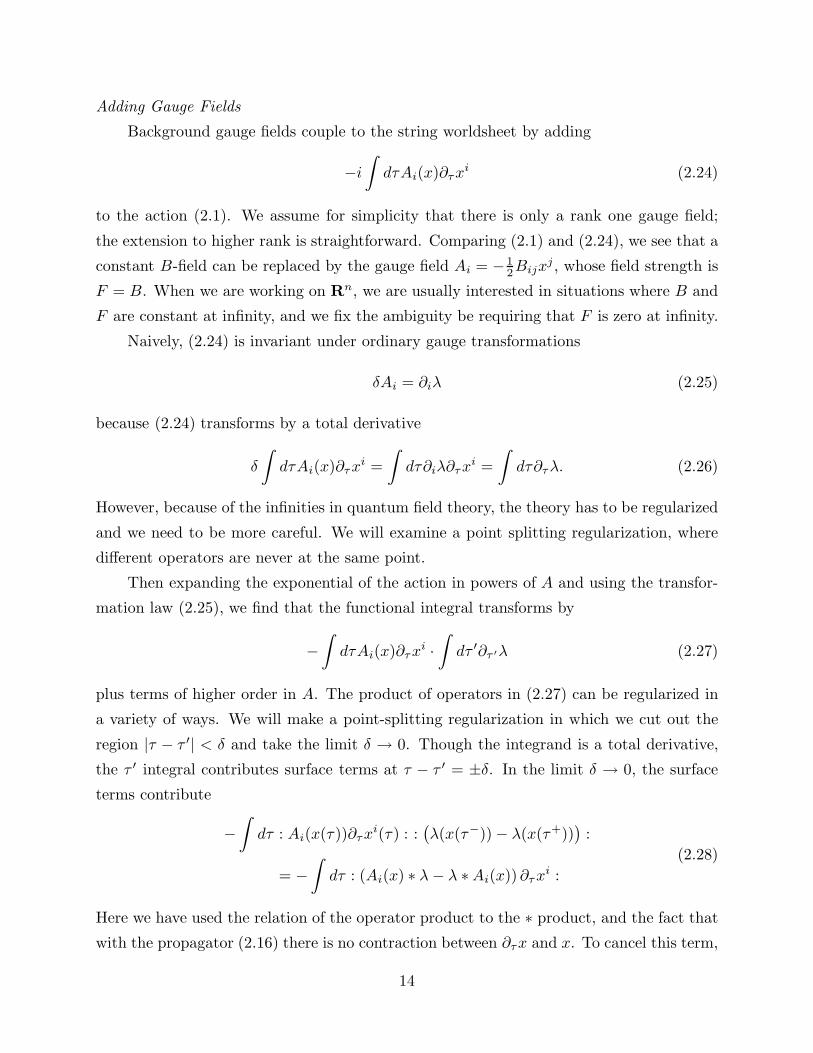
Adding Gauge Fields

Background gauge fields couple to the string worldsheet by adding

−i∫dτAi(x)∂τx

i (2.24)

to the action (2.1). We assume for simplicity that there is only a rank one gauge field;

the extension to higher rank is straightforward. Comparing (2.1) and (2.24), we see that a

constant B-field can be replaced by the gauge field Ai = −12Bijx

j , whose field strength is

F = B. When we are working on Rn, we are usually interested in situations where B and

F are constant at infinity, and we fix the ambiguity be requiring that F is zero at infinity.

Naively, (2.24) is invariant under ordinary gauge transformations

δAi = ∂iλ (2.25)

because (2.24) transforms by a total derivative

δ

∫dτAi(x)∂τx

i =

∫dτ∂iλ∂τx

i =

∫dτ∂τλ. (2.26)

However, because of the infinities in quantum field theory, the theory has to be regularized

and we need to be more careful. We will examine a point splitting regularization, where

different operators are never at the same point.

Then expanding the exponential of the action in powers of A and using the transfor-

mation law (2.25), we find that the functional integral transforms by

−∫dτAi(x)∂τx

i ·∫dτ ′∂τ ′λ (2.27)

plus terms of higher order in A. The product of operators in (2.27) can be regularized in

a variety of ways. We will make a point-splitting regularization in which we cut out the

region |τ − τ ′| < δ and take the limit δ → 0. Though the integrand is a total derivative,

the τ ′ integral contributes surface terms at τ − τ ′ = ±δ. In the limit δ → 0, the surface

terms contribute

−∫dτ : Ai(x(τ))∂τx

i(τ) : :(λ(x(τ−)) − λ(x(τ+))

):

= −∫dτ : (Ai(x) ∗ λ− λ ∗Ai(x)) ∂τx

i :

(2.28)

Here we have used the relation of the operator product to the ∗ product, and the fact that

with the propagator (2.16) there is no contraction between ∂τx and x. To cancel this term,

14

we must add another term to the variation of the gauge field; the theory is invariant not

under (2.25), but under

δAi = ∂iλ+ iλ ∗ Ai − iAi ∗ λ. (2.29)

This is the gauge invariance of noncommutative Yang-Mills theory, and in recognition of

that fact we henceforth denote the gauge field in the theory defined with point splitting

regularization as A. A sigma model expansion with Pauli-Villars regularization would

have preserved the standard gauge invariance of open string gauge field, so whether we get

ordinary or noncommutative gauge fields depends on the choice of regulator.

We have made this derivation to lowest order in A, but it is straightforward to go to

higher orders. At the n-th order in A, the variation is

in+1

n!

∫A(x(t1)) . . . A(x(tn))∂tλ(x(t))

+in+1

(n− 1)!

∫A(x(t1)) . . . A(x(tn−1))

(λ ∗ A(x(tn)) − A ∗ λ(x(tn))

),

(2.30)

where the integration region excludes points where some t’s coincide. The first term in

(2.30) arises by using the naive gauge transformation (2.25), and expanding the action to

n-th order in A and to first order in λ. The second term arises from using the correction

to the gauge transformation in (2.29) and expanding the action to the same order in A

and λ. The first term can be written as

in+1

n!

∑

j

∫A(x(t1)) . . . A(x(tj−1))A(x(tj+1)) . . . A(x(tn))

(A ∗ λ(x(tj)) − λ ∗ A(x(tj))

)

=in+1

(n− 1)!

∫A(x(t1)) . . . A(x(tn−1))

(A ∗ λ(x(tn)) − λ ∗ A(x(tn))

),

(2.31)

making it clear that (2.30) vanishes. Therefore, there is no need to modify the gauge

transformation law (2.29) at higher orders in A.

Let us return to the original theory before taking the zero slope limit (2.14), and

examine the correlation functions of the physical vertex operators of gauge fields

V =

∫ξ · ∂xeip·x (2.32)

These operators are physical when

ξ · p = p · p = 0, (2.33)

15

where the dot product is with the open string metric G (2.5). We will do an explicit

calculation to illustrate the statement that the B dependence of the S-matrix, for fixed G,

consists of replacing ordinary products with ∗ products. Using the conditions (2.33) and

momentum conservation, the three point function is

⟨ξ1 · ∂xeip1·x(τ1) ξ2 · ∂xeip2·x(τ2) ξ3 · ∂xeip3·x(τ3)

⟩∼ 1

(τ1 − τ2)(τ2 − τ3)(τ3 − τ1)

·(ξ1 · ξ2p2 · ξ3 + ξ1 · ξ3p1 · ξ2 + ξ2 · ξ3p3 · ξ1 + 2α′p3 · ξ1p1 · ξ2p2 · ξ3

)

· e− i2(p1

i θijp2jǫ(τ1−τ2)+p2

i θijp3jǫ(τ2−τ3)+p3

i θijp1jǫ(τ3−τ1)).

(2.34)

This expression should be multiplied by the Chan-Paton matrices. The order of these

matrices is correlated with the order of τn. Therefore, for a given order of these matrices

we should not sum over different orders of τn. Generically, the vertex operators (2.32)

should be integrated over τn, but in the case of the three point function on the disc, the

gauge fixing of the SL(2;R) conformal group cancels the integral over the τ ’s. All we need

to do is to remove the denominator (τ1 − τ2)(τ2 − τ3)(τ3 − τ1). This leads to the amplitude

(ξ1 · ξ2p2 · ξ3 + ξ1 · ξ3p1 · ξ2 + ξ2 · ξ3p3 · ξ1 + 2α′p3 · ξ1p1 · ξ2p2 · ξ3

)· e− i

2 p1i θijp2

j . (2.35)

The first three terms are the same as the three point function evaluated with the

action(α′)

3−p2

4(2π)p−2Gs

∫ √detGGii′Gjj′

Tr Fij ∗ Fi′j′ , (2.36)

where Gs is the string coupling and

Fij = ∂iAj − ∂jAi − iAi ∗ Aj + iAj ∗ Ai (2.37)

is the noncommutative field strength. The normalization is the standard normalization

in open string theory. The effective open string coupling constant Gs in (2.36) can differ

from the closed string coupling constant gs. We will determine the relation between them

shortly. The last term in (2.35) arises from the (∂A)3 part of a term α′F 3 in the effective

action. This term vanishes for α′ → 0 (and in any event is absent for superstrings).

Gauge invariance of (2.36) is slightly more subtle than in ordinary Yang-Mills theory.

Since under gauge transformations δF = iλ ∗ F − iF ∗ λ, the gauge variation of F ∗ F is

not zero. But this gauge variation is λ ∗ (iF ∗ F ) − (iF ∗ F ) ∗ λ, and the integral of this

vanishes by virtue of (1.3). Notice that, because the scaling in (2.14) keeps all components

of G fixed as ǫ→ 0, (2.36) is uniformly valid whether the rank of B is p+ 1 or smaller.

16

The three point function (2.34) can easily be generalized to any number of gauge

fields. Using (2.10)

⟨∏

n

ξn · ∂xeipn·x(τn)

⟩

G,θ

= e− i

2

∑n>m

pni θijpm

j ǫ(τn−τm)

⟨∏

n

ξn · ∂xeipn·x(τn)

⟩

G,θ=0

.

(2.38)

This illustrates the claim that when the effective action is expressed in terms of the open

string variables G, θ and Gs (as opposed to g, B and gs), θ appears only in the ∗ product.

The construction of the effective Lagrangian from the S-matrix elements is always

subject to a well-known ambiguity. The S-matrix is unchanged under field redefinitions

in the effective Lagrangian. Therefore, there is no canonical choice of fields. The vertex

operators determine the linearized gauge symmetry, but field redefinitions Ai → Ai+fi(Aj)

can modify the nonlinear terms. It is conventional in string theory to define an effective

action for ordinary gauge fields with ordinary gauge invariances that generates the S-

matrix. In this formulation, the B-dependence of the effective action is very simple: it

is described by everywhere replacing F by F + B. (This is manifest in the sigma model

approach that we mention presently.)

We now see that it is also natural to generate the S-matrix from an effective action

written for noncommutative Yang-Mills fields. In this description, the B-dependence is

again simple, though different. For fixed G and Gs, B affects only θ, which determines the

∗ product. Being able to describe the same S-matrix with the two kinds of fields means

that there must be a field redefinition of the form Ai → Ai + fi(Aj), which relates them.

This freedom to write the effective action in terms of different fields has a counterpart

in the sigma model description of string theory. Here we can use different regularization

schemes. With Pauli-Villars regularization (such as the regularization we use in section

2.3), the theory has ordinary gauge symmetry, as the total derivative in (2.26) integrates

to zero. Additionally, with such a regularization, the effective action can depend on B and

F only in the combination F + B, since there is a symmetry A → A + Λ, B → B − dΛ,

for any one-form Λ. With point-splitting regularization, we have found noncommutative

gauge symmetry, and a different description of the B-dependence.

The difference between different regularizations is always in a choice of contact terms;

theories defined with different regularizations are related by coupling constant redefini-

tion. Since the coupling constants in the worldsheet Lagrangian are the spacetime fields,

the two descriptions must be related by a field redefinition. The transformation from

17

ordinary to noncommutative Yang-Mills fields that we will describe in section 3 is thus

an example of a transformation of coupling parameters that is required to compare two

different regularizations of the same quantum field theory.

In the α′ → 0 limit (2.14), the amplitudes and the effective action are simplified. For

example, the α′F 3 term coming from the last term in the amplitude (2.35) is negligible in

this limit. More generally, using dimensional analysis and the fact that the θ dependence

is only in the definition of the ∗ product, it is clear that all higher dimension operators

involve more powers of α′. Therefore they can be neglected, and the F 2 action (2.36)

becomes exact for α′ → 0.

The lack of higher order corrections to (2.36) can also be understood as follows. In the

limit (2.14), there are no on-shell vertex operators with more derivatives of x, which would

correspond to massive string modes. Since there are no massive string modes, there cannot

be corrections to (2.36). As a consistency check, note that there are no poles associated

with such operators in (2.22) or in (2.38) in our limit.

All this is standard in the zero slope limit, and the fact that the action for α′ → 0

reduces to F 2 is quite analogous to the standard reduction of open string theory to ordinary

Yang-Mills theory for α′ → 0. The only novelty in our discussion is the fact that for B 6= 0,

we have to take α′ → 0 keeping fixed G rather than g. Even before taking the α′ → 0

limit, the effective action, as we have seen, can be written in terms of the noncommutative

variables. The role of the zero slope limit is just to remove the higher order corrections to

F 2 from the effective action.

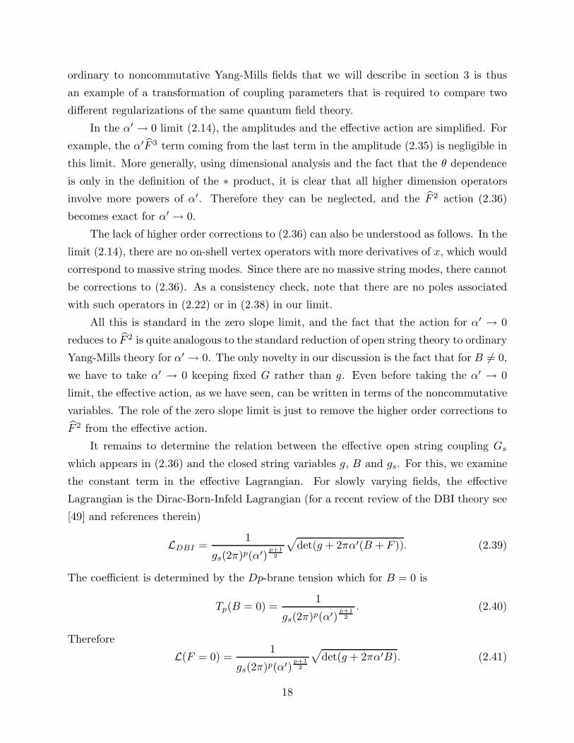
It remains to determine the relation between the effective open string coupling Gs

which appears in (2.36) and the closed string variables g, B and gs. For this, we examine

the constant term in the effective Lagrangian. For slowly varying fields, the effective

Lagrangian is the Dirac-Born-Infeld Lagrangian (for a recent review of the DBI theory see

[49] and references therein)

LDBI =1

gs(2π)p(α′)p+12

√det(g + 2πα′(B + F )). (2.39)

The coefficient is determined by the Dp-brane tension which for B = 0 is

Tp(B = 0) =1

gs(2π)p(α′)p+12

. (2.40)

Therefore

L(F = 0) =1

gs(2π)p(α′)p+12

√det(g + 2πα′B). (2.41)

18

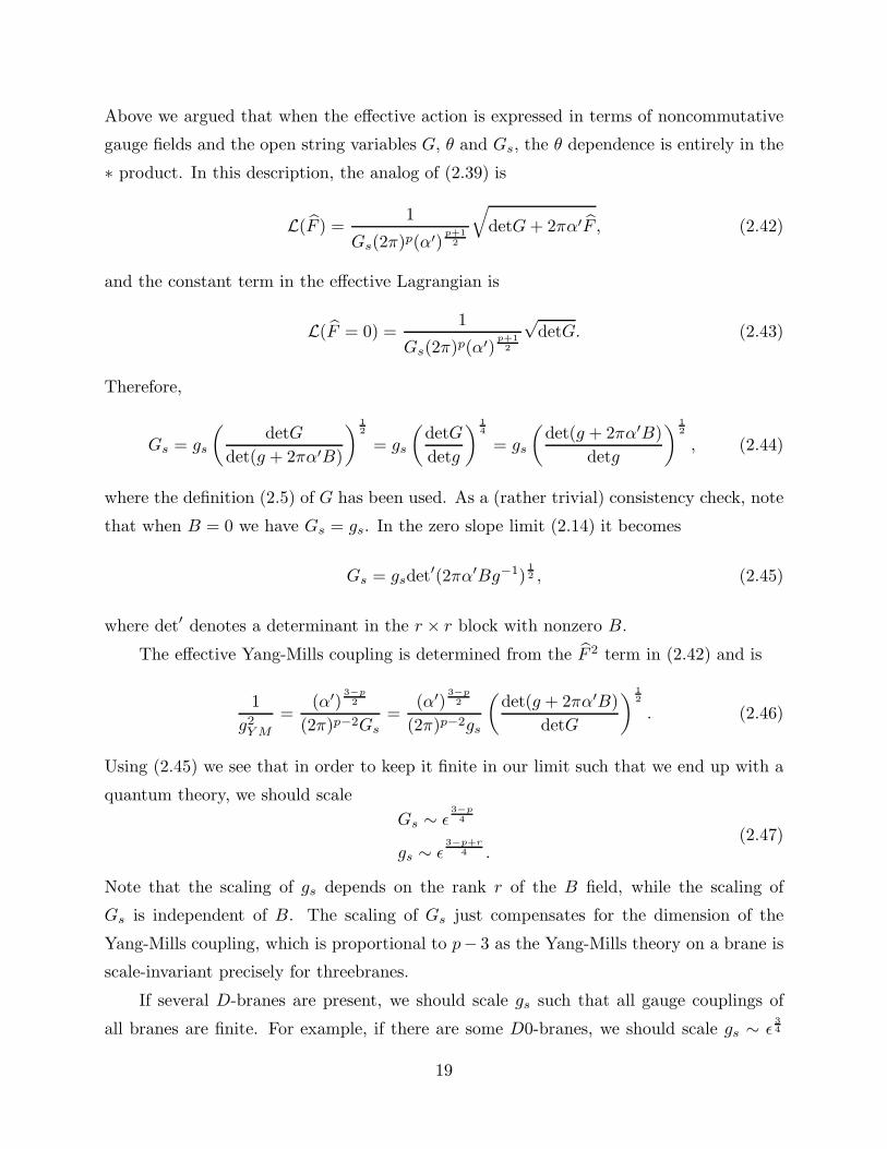
Above we argued that when the effective action is expressed in terms of noncommutative

gauge fields and the open string variables G, θ and Gs, the θ dependence is entirely in the

∗ product. In this description, the analog of (2.39) is

L(F ) =1

Gs(2π)p(α′)p+12

√detG+ 2πα′F , (2.42)

and the constant term in the effective Lagrangian is

L(F = 0) =1

Gs(2π)p(α′)p+12

√detG. (2.43)

Therefore,

Gs = gs

(detG

det(g + 2πα′B)

) 12

= gs

(detG

detg

) 14

= gs

(det(g + 2πα′B)

detg

) 12

, (2.44)

where the definition (2.5) of G has been used. As a (rather trivial) consistency check, note

that when B = 0 we have Gs = gs. In the zero slope limit (2.14) it becomes

Gs = gsdet′(2πα′Bg−1)12 , (2.45)

where det′ denotes a determinant in the r × r block with nonzero B.

The effective Yang-Mills coupling is determined from the F 2 term in (2.42) and is

1

g2Y M

=(α′)

3−p2

(2π)p−2Gs=

(α′)3−p2

(2π)p−2gs

(det(g + 2πα′B)

detG

) 12

. (2.46)

Using (2.45) we see that in order to keep it finite in our limit such that we end up with a

quantum theory, we should scale

Gs ∼ ǫ3−p4

gs ∼ ǫ3−p+r

4 .(2.47)

Note that the scaling of gs depends on the rank r of the B field, while the scaling of

Gs is independent of B. The scaling of Gs just compensates for the dimension of the

Yang-Mills coupling, which is proportional to p− 3 as the Yang-Mills theory on a brane is

scale-invariant precisely for threebranes.

If several D-branes are present, we should scale gs such that all gauge couplings of

all branes are finite. For example, if there are some D0-branes, we should scale gs ∼ ǫ34

19

(p = r = 0 in (2.47)). In this case, all branes for which p > r can be treated classically,

and branes with p = r are quantum.

If we are on a torus, then the limit (2.14) with gij → 0 and Bij fixed is essentially the

limit used in [4]. This limit takes the volume to zero while keeping fixed the periods of B.

On the other hand, if we are on Rn, then by rescaling the coordinates, instead of taking

gij → 0 with Bij fixed, one could equivalently keep gij fixed and take Bij → ∞. (Scaling

the coordinates on Tn changes the periodicity, and therefore it is more natural to scale

the metric in this case.) In this sense, the α′ → 0 limit can, on Rn, be interpreted as a

large B limit.

It is crucial that gij is taken to zero with fixed Gij . The latter is the metric appearing

in the effective Lagrangian. Therefore, either on Rn or on a torus, all distances measured

with the metric g scale to zero, but the noncommutative theory is sensitive to the metric

G, and with respect to this metric the distances are fixed. This is the reason that we end

up with finite distances even though the closed string metric g is taken to zero.

2.2. Worldsheet Supersymmetry

We now add fermions to the theory and consider worldsheet supersymmetry. Without

background gauge fields we have to add to the action (2.1)

i

4πα′

∫

Σ

(gijψ

i∂ψj + gijψi∂ψ

j)

(2.48)

and the boundary conditions are

gij(ψj − ψ

j) + 2πα′Bij(ψ

j + ψj)∣∣z=z

= 0 (2.49)

(ψ is not the complex conjugate of ψ). The action and the boundary conditions respect

the supersymmetry transformations

δxi = −iη(ψi + ψi)

δψi = η∂xi

δψi= η∂xi,

(2.50)

In studying sigma models, the boundary interaction (2.24) is typically extended to

LA = −i∫dτ(Ai(x)∂τx

i − iFijΨiΨj)

(2.51)

20

with Fij = ∂iAj − ∂jAi and

Ψi =1

2(ψi + ψ

i) =

(1

g − 2πα′Bg

)i

j

ψj . (2.52)

The expression (2.51) seems to be invariant under (2.50) because its variation is a

total derivative

δ

∫dτ(Ai(x)∂τx

i − iFijΨiΨj)

= −2iη

∫dτ∂τ (AiΨ

i). (2.53)

However, as in the derivation of (2.28), with point splitting regularization, a total derivative

such as the one in (2.53) can contribute a surface term. In this case, the surface term is

obtained by expanding the exp(−LA) term in the path integral in powers of A. The

variation of the path integral coming from (2.53) reads, to first order in LA,

i

∫dτ

∫dτ ′(Ai∂τx

i(τ) − iFijΨiΨj(τ)

) (−2iη∂τ ′AkΨk(τ ′)

). (2.54)

With point splitting regularization, one picks up surface terms as τ ′ → τ+ and τ ′ → τ−,

similar to those in (2.28). The surface terms can be canceled by the supersymmetric

variation of an additional interaction term∫dτAi ∗AjΨ

iΨj(τ), and the conclusion is that

with point-splitting regularization, (2.51) should be corrected to

−i∫dτ(Ai(x)∂τx

i − iFijΨiΨj)

(2.55)

with F the noncommutative field strength (2.37).

Once again, if supersymmetric Pauli-Villars regularization were used (an example of

an explicit regularization procedure will be given presently in discussing instantons), the

more naive boundary coupling (2.51) would be supersymmetric. Whether “ordinary” or

“noncommutative” gauge fields and symmetries appear in the formalism depends on the

regularization used, so there must be a transformation between them.

2.3. Instantons On Noncommutative R4

As we mentioned in the introduction, one of the most fascinating applications of

noncommutative Yang-Mills theory has been to instantons on R4. Given a system of N

parallel D-branes with worldvolume R4, one can study supersymmetric configurations in

the U(N) gauge theory. (Actually, most of the following discussion applies just as well if R4

21

is replaced by Tn ×R4−n for some n.) In classical Yang-Mills theory, such a configuration

is an instanton, that is a solution of F+ = 0. (For any two-form on R4 such as the Yang-

Mills curvature F , we write F+ and F− for the self-dual and anti-self-dual projections.)

So the objects we want are a stringy generalization of instantons. A priori one would

expect that classical instantons would be a good approximation to stringy instantons only

when the instanton scale size is very large compared to√α′. However, we will now argue

that with a suitable regularization of the worldsheet theory, the classical or field theory

instanton equation is exact if B = 0. This implies that with any regularization, the stringy

and field theory instanton moduli spaces are the same. The argument, which is similar

to an argument about sigma models with K3 target [50], also suggests that for B 6= 0,

the classical instanton equations and moduli space are not exact. We have given some

arguments for this assertion in the introduction, and will give more arguments below and

in the rest of the paper.

At B = 0, the free worldsheet theory in bulk

S =1

4πα′

∫

Σ

(gij∂ax

i∂axi + igijψi∂ψj + igijψ

i∂ψ

j)

(2.56)

actually has a (4, 4) worldsheet supersymmetry. This is a consequence of the N = 1

worldsheet supersymmetry described in (2.50) plus an R symmetry group. In fact, we

have a symmetry group SO(4)L acting on the ψi and another SO(4)R acting on ψi. We

can decompose SO(4)L = SU(2)L,+ × SU(2)L,−, and likewise SO(4)R = SU(2)R,+ ××SU(2)R,−. SU(2)R,+, together with the N = 1 supersymmetry in (2.50), generates an

N = 4 supersymmetry of the right-movers, and SU(2)L,+, together with (2.50), likewise

generates an N = 4 supersymmetry of left-movers. So altogether in bulk we get an

N = (4, 4) free superconformal model. Of course, we could replace SU(2)R,+ by SU(2)R,−

or SU(2)L,+ by SU(2)L,−, so altogether the free theory has (at least) four N = (4, 4)

superconformal symmetries. But for the instanton problem, we will want to focus on just

one of these extended superconformal algebras.

Now consider the case that Σ has a boundary, but with B = 0 and no gauge fields

coupled to the boundary. The boundary conditions on the fermions are, from (2.49),

ψj = ψj. This breaks SO(4)L × SO(4)R down to a diagonal subgroup SO(4)D =

SU(2)D,+ × SU(2)D,− (here SU(2)D,+ is a diagonal subgroup of SU(2)L,+ × SU(2)R,+,

and likewise for SU(2)D,−). We can define an N = 4 superconformal algebra in which

the R-symmetry is SU(2)D,+ (and another one with R-symmetry SU(2)D,−). As is usual

22

for open superstrings, the currents of this N = 4 algebra are mixtures of left and right

currents from the underlying N = (4, 4) symmetry in bulk.

Now let us include a boundary interaction as in (2.51):

LA = −i∫dτ(Ai(x)∂τx

i − iFijΨiΨj). (2.57)

The condition that the boundary interaction preserves some spacetime supersymmetry is

that the theory with this interaction is still an N = 4 theory. This condition is easy

to implement, at the classical level. The Ψi transform as (1/2, 1/2) under SU(2)D,+ ×SU(2)D,−. The FijΨ

iΨj coupling in LA transforms as the antisymmetric tensor product of

this representation with itself, or (1, 0)⊕(0, 1), where the two pieces multiply, respectively,

F+ and F−, the self-dual and anti-self-dual parts of F . Hence, the condition that LA be

invariant under SU(2)D,+ is that F+ = 0, in other words that the gauge field should be an

instanton. For invariance under SU(2)D,− we need F− = 0, an anti-instanton. Thus, at

the classical level, an instanton or anti-instanton gives an N = 4 superconformal theory,3

and hence a supersymmetric or BPS configuration.

To show that this conclusion is valid quantum mechanically, we need a regularization

that preserves (global) N = 1 supersymmetry and also the SO(4)D symmetry. This

can readily be provided by Pauli-Villars regularization. First of all, the fields xi, ψi, ψi,

together with auxiliary fields F i, can be interpreted in the standard way as components

of N = 1 superfields Φi, i = 1, . . . , 4.

To carry out Pauli-Villars regularization, we introduce two sets of superfields Ci and

Ei, where Ei are real-valued and Ci takes values in the same space (R4 or more generally

Tn × R4−n) that Φi does, and we write Φi = Ci − Ei. For Ci and Ei, we consider the

following Lagrangian:

L =

∫d2xd2θ

(ǫαβDαC

iDβCi)−∫d2xd2θ

(ǫαβDαE

iDβEi +M2(Ei)2

). (2.58)

This regularization of the bulk theory is manifestly invariant under global N = 1 super-

symmetry. But since it preserves an SO(4)D (which under which all left and right fermions

in C or E transform as (1/2, 1/2)), it actually preserves a global N = 4 supersymmetry.

3 Our notation is not well adapted to nonabelian gauge theory. In this case, the factor e−LA

in the path integral must be reinterpreted as a trace TrP exp∮

∂Σ

(iAi∂τxi + FijΨ

iΨj)

where the

exponent is Lie algebra valued. This preserves SU(2)D,± if F± = 0.

23

This symmetry can be preserved in the presence of boundaries. We simply consider

free boundary conditions for both Ci and Ei. The usual short distance singularity is absent

in the Φi propagator (as it cancels between Ci and Ei). Now, include a boundary coupling

to gauge fields by the obvious superspace version of (2.51):

LA = −i∫dτdθ Ai(Φ)DΦi = −i

∫dτ(Ai(x)∂τx

i − iFijΨiΨj). (2.59)

Classically (as is clear from the second form, which arises upon doing the θ integral), this

coupling preserves SU(2)D,+ if F+ = 0, or SU(2)D,− if F− = 0. Because of the absence of

a short distance singularity in the Φ propagator, all Feynman diagrams are regularized.4

Hence, for every classical instanton, we get a two-dimensional quantum field theory with

global N = 4 supersymmetry.

If this theory flows in the infrared to a conformal field theory, this theory is N = 4

superconformal and hence describes a configuration with spacetime supersymmetry. On

the other hand, the global N = 4 supersymmetry, which holds precisely if F+ = 0,

means that any renormalization group flow that occurs as M → ∞ would be a flow

on classical instanton moduli space. Such a flow would mean that stringy corrections

generate a potential on instanton moduli space. But there is too much supersymmetry

for this, and therefore there is no flow on the space; i.e. different classical instantons

lead to distinct conformal field theories. We conclude that, with this regularization, every

classical instanton corresponds in a natural way to a supersymmetric configuration in string

theory or in other words to a stringy instanton. Thus, with this regularization, the stringy

instanton equation is just F+ = 0. Since the moduli space of conformal field theories is

independent of the regularization, it also follows that with any regularization, the stringy

instanton moduli space coincides with the classical one.

Turning On B

Now, let us reexamine this issue in the presence of a constant B field. The boundary

condition required by supersymmetry was given in (2.49):

(gij + 2πα′Bij)ψj = (gij − 2παBij)ψ

j. (2.60)

4 In most applications, Pauli-Villars regularization fails to regularize the one-loop diagrams,

because it makes the vertices worse while making the propagators better. The present problem

has the unusual feature that Pauli-Villars regularization eliminates the short distance problems

even from the one-loop diagrams.

24

To preserve (2.60), if one rotates ψi by an SO(4) matrix h, one must rotate ψi

with

a different SO(4) matrix h. The details of the relation between h and h will be explored

below, in the context of point-splitting regularization. At any rate, (2.60) does preserve

a diagonal subgroup SO(4)D,B of SO(4)L × SO(4)R, but as the notation suggests, which

diagonal subgroup it is depends on B.

The Pauli-Villars regularization introduced above preserves SO(4)D, which for B 6= 0

does not coincide with SO(4)D,B. The problem arises because the left and right chiral

fermions in the regulator superfields Ei are coupled by the mass term in a way that breaks

SO(4)L × SO(4)R down to SO(4)D, but they are coupled by the boundary condition in a

way that breaks SO(4)L × SO(4)R down to SO(4)D,B. Thus, the argument that showed

that classical instanton moduli space is exact for B = 0 fails for B 6= 0.

This discussion raises the question of whether a different regularization would enable

us to prove the exactness of classical instantons for B 6= 0. However, a very simple

argument mentioned in the introduction shows that one must expect stringy corrections

to instanton moduli space when B 6= 0. In fact, if B+ 6= 0, a configuration containing

a threebrane and a separated −1-brane is not BPS (we will explore it in section 5), so

the small instanton singularity that is familiar from classical Yang-Mills theory should be

absent when B+ 6= 0.

It has been proposed [35,38] that the stringy instantons at B+ 6= 0 are the instantons

of noncommutative Yang-Mills theory, that is the solutions of F+ = 0 with a suitable ∗product. We can now make this precise in the α′ → 0 limit. In this limit, the effective

action is, as we have seen, F 2, with the indices in F contracted by the open string metric

G. In this theory, the condition for a gauge field to leave unbroken half of the linearly

realized supersymmetry on the branes is F+ = 0, where the projection of F to selfdual and

antiselfdual parts is made with respect to the open string metric G, rather than the closed

string metric g. Hence, at least in the α′ = 0 limit, BPS configurations are described by

noncommutative instantons, as has been suggested in [35,38]. If we are on R4, then, as

shown in [35], deforming the classical instanton equation F+ = 0 to the noncommutative

instanton equation F+ = 0 has the effect of adding a Fayet-Iliopoulos (FI) constant term

to the ADHM equations, removing the small instanton singularity5. The ADHM equations

5 Actually, it was assumed in [35] that θ is self-dual. The general situation, as we will show

at the end of section 5, is that the small instanton singularity is removed precisely if B+ 6= 0, or

equivalently θ+ 6= 0.

25

with the FI term have a natural interpretation in terms of the DLCQ description of the

six-dimensional (2, 0) theory [37], and have been studied mathematically in [41].

What happens if B 6= 0 but we do not take the α′ → 0 limit? In this case, the stringy

instanton moduli space must be a hyper-Kahler deformation of the classical instanton

moduli space, with the small instanton singularities eliminated if B+ 6= 0, and reducing to

the classical instanton moduli space for instantons of large scale size if we are on R4. We

expect that the most general hyper-Kahler manifold meeting these conditions is the moduli

space of noncommutative instantons, with some θ parameter and with some effective metric

on spacetime G.6

Details For Instanton Number One

Though we do not know how to prove this in general, one can readily prove it by

hand for the case of instantons of instanton number one on R4. The ADHM construction

for such instantons, with gauge group U(N), expresses the moduli space as the moduli

space of vacua of a U(1) gauge theory with N hypermultiplets Ha of unit charge (times a

copy of R4 for the instanton position). In the α′ → 0 limit with non-zero B, there is a FI

term. If we write the hypermultiplets Ha, in a notation that makes manifest only half the

supersymmetry, as a pair of chiral superfields Aa, Ba, with respective charges 1,−1, then

the ADHM equations read ∑

a

AaBa = ζc.

∑

a

|Aa|2 −∑

a

|Ba|2 = ζ.(2.61)

One must divide by Aa → eiαAa, Ba → e−iαBa. Here ζc is a complex constant, and ζ a

real constant. ζc and ζ are the FI parameters. The real and imaginary part of ζc, together

with ζ, transform as a triplet of an SU(2) R-symmetry group, which is broken to U(1)

(rotations of ζc) by our choice of writing the equations in terms of chiral superfields. To

determine the topology of the moduli space M, we make an SU(2)R transformation (or a

judicious choice of Aa and Ba) to set ζc = 0 and ζ > 0. Then, if we set Ba = 0, the Aa,

modulo the action of U(1), determine a point in CPN ; the equation∑

aAaBa = 0 means

that the Ba determine a cotangent vector of CPN , so M is the cotangent bundle T ∗CPN .

6 The effective metric on spacetime must be hyper-Kahler for supersymmetry, so it is a flat

metric if we are on R4 or T

n×R4−n, or a hyper-Kahler metric if we are bold enough to extrapolate

the discussion to a K3 manifold or a Taub-NUT or ALE space.

26

The second homology group of M is of rank one, being generated by a two-cycle in

CPN . Moduli space of hyper-Kahler metrics is parametrized by the periods of the three

covariantly constant two-forms I, J,K. As there is only one period, there are precisely

three real moduli, namely ζ, Re ζc, and Im ζc.

Hence, at least for instanton number one, the stringy instanton moduli space on R4,

for any B, must be given by the solutions of F+ = 0, with some effective metric on

spacetime and some effective theta parameter. It is tempting to believe that these may be

the metric and theta parameter found in (2.5) from the open string propagator.

Noncommutative Instantons And N = 4 Supersymmetry

We now return to the question of what symmetries are preserved by the boundary

condition (2.60). We work in the α′ → 0 limit, so that we know the boundary couplings

and the gauge invariances precisely. The goal is to show, by analogy with what happened

for B = 0, that noncommutative gauge fields that are self-dual with respect to the open

string metric lead to N = 4 worldsheet superconformal symmetry.

It is convenient to introduce a vierbein eia for the closed string metric Thus g−1 = eet

(et is the transpose of e) or gij =∑

a eiae

ja. Then, we express the fermions in terms of the

local Lorentz frame in spacetime

ψi = eiaχ

a, ψi= ei

aχa. (2.62)

The SO(4)L × SO(4)R automorphism group of the supersymmetry algebra rotates these

four fermions by χ→ hχ and χ→ hχ. The boundary conditions (2.60) breaks SO(4)L ×SO(4)R to a diagonal subgroup SO(4)D,B defined by

h = e−1 1

g − 2πα′B(g + 2πα′B)ehe−1 1

g + 2πα′B(g − 2πα′B)e. (2.63)

In terms of χ and χ, the boundary coupling of the original fermions (2.55) becomes

χtetg1

g + 2πα′BF

1

g − 2πα′Bgeχ. (2.64)

We have used (2.52) to express Ψ in terms of ψ, and (2.62) to express ψ in terms of χ.

Under SO(4)D,B, this coupling transforms as

χtetg1

g + 2πα′BF

1

g − 2πα′Bgeχ→ χthtetg

1

g + 2πα′BF

1

g − 2πα′Bgehχ, (2.65)

27

and the theory is invariant under the subgroup of SO(4)D,B for which

etg1

g + 2πα′BF

1

g − 2πα′Bge = htetg

1

g + 2πα′BF

1

g − 2πα′Bgeh. (2.66)

In order to analyze the consequences of this equation, we define a vierbein for the open

string metric by the following very convenient formula:

E =1

g − 2πα′Bge. (2.67)

To verify that this is a vierbein, we compute

EEt =1

g − 2πα′Bg

1

g + 2πα′B=

1

g + 2πα′Bg

1

g − 2πα′B= G−1. (2.68)

In terms of E, (2.66) reads

EtFE = htEtFEh. (2.69)

For this equation to hold for h in an SU(2) subgroup of SO(4)D,B, EtFEt must be

selfdual, or anti-selfdual, with respect to the trivial metric of the local Lorentz frame. This

is equivalent to F being selfdual or anti-selfdual with respect to the open string metric G.

Thus, we have shown that the boundary interaction preserves an SU(2) R symmetry, and

hence an N = 4 superconformal symmetry, if F+ = 0 or F− = 0 with respect to the open

string metric.

3. Noncommutative Gauge Symmetry vs. Ordinary Gauge Symmetry

We have by now seen that ordinary and noncommutative Yang-Mills fields arise from

the same two-dimensional field theory regularized in different ways. Consequently, there

must be a transformation from ordinary to noncommutative Yang-Mills fields that maps

the standard Yang-Mills gauge invariance to the gauge invariance of noncommutative Yang-

Mills theory. Moreover, this transformation must be local in the sense that to any finite

order in perturbation theory (in θ) the noncommutative gauge fields and gauge parameters

are given by local differential expressions in the ordinary fields and parameters.

At first sight, it seems that we want a local field redefinition A = A(A, ∂A, ∂2A, . . . ; θ)

of the gauge fields, and a simultaneous reparametrization λ = λ(λ, ∂λ, ∂2λ, . . . ; θ) of the

gauge parameters that maps one gauge invariance to the other. However, this must be

relaxed. If there were such a map intertwining with the gauge invariances, it would follow

28

that the gauge group of ordinary Yang-Mills theory is isomorphic to the gauge group of

noncommutative Yang-Mills theory. This is not the case. For example, for rank one, the

ordinary gauge group, which acts by

δAi = ∂iλ, (3.1)

is Abelian, while the noncommutative gauge invariance, which acts by

δAi = ∂iλ+ iλ ∗Ai − iAi ∗ λ, (3.2)

is nonabelian. An Abelian group cannot be isomorphic to a nonabelian group, so no

redefinition of the gauge parameter can map the ordinary gauge parameter to the noncom-

mutative one while intertwining with the gauge symmetries.

What we actually need is less than an identification between the two gauge groups. To

do physics with gauge fields, we only need to know when two gauge fields A and A′ should

be considered gauge-equivalent. We do not need to select a particular set of generators of

the gauge equivalence relation – a gauge group that generates the equivalence relation7.

In the problem at hand, it turns out that we can map A to A in a way that preserves the

gauge equivalence relation, even though the two gauge groups are different.

What this means in practice is as follows. We will find a mapping from ordinary

gauge fields A to noncommutative gauge fields A which is local to any finite order in θ and

has the following further property. Suppose that two ordinary gauge fields A and A′ are

equivalent by an ordinary gauge transformation by U = exp(iλ). Then, the corresponding

noncommutative gauge fields A and A′ will also be gauge-equivalent, by a noncommutative

gauge transformation by U = exp(iλ). However, λ will depend on both λ and A. If λ were

a function of λ only, the ordinary and noncommutative gauge groups would be the same;

since λ is a function of A as well as λ, we do not get any well-defined mapping between

the gauge groups, and we get an identification only of the gauge equivalence relations.

Note that the situation that we are considering here is the opposite of a gauge theory

in which the gauge group has field-dependent structure constants or only closes on shell.

This means (see [51] for a fuller explanation) that one has a well-defined gauge equivalence

7 Fadde’ev-Popov quantization of gauge theories is formulated in terms of the gauge group,

but in the more general Batalin-Vilkovisky approach to quantization, the emphasis is on the

equivalence relation generated by the gauge transformations. For a review of this approach, see

[51].

29

relation, but the equivalence classes are not the orbits of any useful group, or are such

orbits only on shell. In the situation that we are considering, there is more than one group

that generates the gauge equivalence relation; one can use either the ordinary gauge group

or (with one’s favorite choice of θ) the gauge group of noncommutative Yang-Mills theory.

Finally, we point out in advance a limitation of the discussion. The arguments in

section 2 (which involved, for example, comparing two different ways of constructing an

α′ expansion of the string theory effective action) show only that ordinary and noncom-

mutative Yang-Mills theory must be equivalent to all finite orders in a long wavelength

expansion. By dimensional analysis, this means that they must be equivalent to all finite

orders in θ. However, it is not clear that the transformation between A and A should

always work nonperturbatively. Indeed, the small instanton problem discussed in section

2.3 seems to give a situation in which the transformation between A and A breaks down,

presumably because the perturbative series that we will construct does not converge.

3.1. The Change Of Variables

Once one is convinced that a transformation of the type described above exists, it is

not too hard to find it. We take the gauge fields to be of arbitrary rank N , so that all fields

and gauge parameters are N ×N matrices (with entries in the ordinary ring of functions

or the noncommutative algebra defined by the ∗ product of functions, as the case may be).

We look for a mapping A(A) and λ(λ,A) such that

A(A) + δλA(A) = A(A+ δλA), (3.3)

with infinitesimal λ and λ. This will ensure that an ordinary gauge transformation of A

by λ is equivalent to a noncommutative gauge transformation of A by λ, so that ordinary

gauge fields that are gauge-equivalent are mapped to noncommutative gauge fields that

are likewise gauge-equivalent. The gauge transformation laws δλ and δλ

were defined at

the end of the introduction. We first work to first order in θ. We write A = A+A′(A) and

λ(λ,A) = λ + λ′(λ,A), with A′ and λ′ local function of λ and A of order θ. Expanding

(3.3) in powers of θ, we find that we need

A′i(A+δλA)−A′

i(A)−∂iλ′−i[λ′, Ai]−i[λ,A′

i] = −1

2θkl(∂kλ∂lAi+∂lAi∂kλ)+O(θ2). (3.4)

In arriving at this formula, we have used the expansion f∗g = fg+ 12iθij∂if∂jg+O(θ2), and

have written the O(θ) part of the ∗ product explicitly on the right hand side. All products

30

in (3.4) are therefore ordinary matrix products, for example [λ′, Ai] = λ′Ai −Aiλ′, where

(as λ′ is of order θ), the multiplication on the right hand side should be interpreted as

ordinary matrix multiplication at θ = 0.

Equation (3.4) is solved by

Ai(A) = Ai +A′i(A) = Ai −

1

4θkl{Ak, ∂lAi + Fli} + O(θ2)

λ(λ,A) = λ+ λ′(λ,A) = λ+1

4θij{∂iλ,Aj} + O(θ2)

(3.5)

where again the products on the right hand side, such as {Ak, ∂lAi} = Ak ·∂lAi +∂lAi ·Ak

are ordinary matrix products. From the formula for A, it follows that

Fij = Fij +1

4θkl (2{Fik, Fjl} − {Ak, DlFij + ∂lFij}) + O(θ2). (3.6)

These formulas exhibit the desired change of variables to first nontrivial order in θ.

By reinterpreting the above formulas, it is a rather short step to write down a dif-

ferential equation that generates the desired change of variables to all finite orders in θ.

Consider the problem of mapping noncommutative gauge fields A(θ) defined with respect

to the ∗ product with one choice of θ, to noncommutative gauge fields A(θ + δθ), defined

for a nearby choice of θ. To first order in δθ, the problem of converting from A(θ) to

A(θ + δθ) is equivalent to what we have just solved. Indeed, apart from associativity, the

only property of the ∗ product that one needs to verify that (3.5) obeys (3.3) to first order

in θ is that for any variation δθij of θ,

δθij ∂

∂θij(f ∗ g) =

i

2δθij ∂f

∂xi∗ ∂g

∂xj(3.7)

at θ = 0. But this is true for any value of θ, as one can verify with a short perusal of the

explicit formula for the ∗ product in (1.2). Hence, adapting the above formulas, we can

write down a differential equation that describes how A(θ) and λ(θ) should change when

θ is varied, to describe equivalent physics:

δAi(θ) = δθkl ∂

∂θklAi(θ) = −1

4δθkl

[Ak ∗ (∂lAi + Fli) + (∂lAi + Fli) ∗ Ak

]

δλ(θ) = δθkl ∂

∂θklλ(θ) =

1

4δθkl (∂kλ ∗Al + Al ∗ ∂kλ)

δFij(θ) = δθkl ∂

∂θklFij(θ) =

1

4δθkl

[2Fik ∗ Fjl + 2Fjl ∗ Fik − Ak ∗

(DlFij + ∂lFij

)

−(DlFij + ∂lFij

)∗ Ak

].

(3.8)

31

On the right hand side, the ∗ product is meant in the generalized sense explained in the

introduction: the tensor product of matrix multiplication with the ∗ product of functions.

This differential equation generates the promised change of variables to all finite orders in

θ. To what extent the series in θ generates by this equation converges is a more delicate

question, beyond the scope of the present paper. The equation is invariant under a scaling

operation in which θ has degree −2 and A and ∂/∂x have degree one, so one can view the

expansion it generates as an expansion in powers of θ for any A, which is how we have

derived it, or as an expansion in powers of A and ∂/∂x for any θ.

The differential equation (3.8) can be solved explicitly for the important case of a rank

one gauge field with constant F . In this case, the equation can be written

δF = −F δθF (3.9)

(the Lorentz indices are contracted as in matrix multiplication). Its solution with the

boundary condition F (θ = 0) = F is

F =1

1 + FθF. (3.10)

From (3.10) we find F in terms of F

F = F1

1 − θF. (3.11)

We can also write these relations as

F − 1

θ= − 1

θ( 1θ + F )θ

. (3.12)

We see that when F = −θ−1 we cannot use the noncommutative description because F

has a pole. Conversely, F is singular when F = θ−1, so in that case, the commutative

description does not exist. Using our identification in the zero slope limit (or in a natural

regularization scheme which will be discussed below) θ = 1B , equations (3.10), (3.11) and

(3.12) become

F = B1

B + FF, (3.13)

F = F1

B − FB (3.14)

and

F −B = −B 1

B + FB. (3.15)

32

So an ordinary Abelian gauge field with constant curvature F and Neveu-Schwarz two-form

field B is equivalent to a noncommutative gauge field with θ = 1/B and the value of F as

in (3.13). When B + F = 0 we cannot use the noncommutative description. It is natural

that this criterion depends only on B + F , since in the description by ordinary Abelian

gauge theory, B and F are mixed by a gauge symmetry, with only the combination B+F

being gauge-invariant.

Application To Instantons

Another interesting application is to instantons in four dimensions. We have argued in

section 2.3 (following [35,38]) that a stringy instanton is a solution of the noncommutative

instanton equation

F+ij = 0. (3.16)

We can evaluate this equation to first nontrivial order in θ using (3.6). Since θkl{Ak, DlFij+

∂lFij}+ = 0 if F+ij = 0, to evaluate the O(θ) deviation of (3.16) from the classical instan-

ton equation F+ij = 0, we can drop those non-gauge-invariant terms in (3.6). We find that

to first order in θ, the noncommutative instanton equation can be written in any of the

following equivalent forms:

0 =F+ij +

1

2

(θkl{Fik, Fjl}

)++ O(θ2)

=F+ij − 1

8

1√detG

ǫrstuFrsFtuGikGjl(θ+)kl + O(θ2)

=F+ij − 1

4(FF )θ+

ij + O(θ2).

(3.17)

Here G is the open string metric, which is used to determine the self-dual parts of F and

θ. In (3.17), we used the facts that F− = O(1) and F+ = O(θ), along with various

identities of SO(4) group theory. For example, in evaluating (θkl{Fik, Fjl})+ to order θ,

one can replace F by F−. According to SO(4) group theory, a product of any number

of anti-selfdual tensors can never make a selfdual tensor, so we can likewise replace θ by

θ+. SO(4) group theory also implies that there is only one self-dual tensor linear in θ+

and quadratic in F−, namely θ+(F−)2, so the O(θ) term in the equation is a multiple of

this. To first order in θ, we can replace (F−)2 by (F−)2 − (F+)2, which is a multiple of

FF = 12√

detGǫrstuFrsFtu; this accounts for the other ways of writing the equation given

in (3.17).

33

In (3.17), we see that to first order, the corrections to the instanton equation depend

only on θ+ and not θ−; in section 5, we explore the extent to which this is true to all

orders.

More Freedom In The Description

What we have learned is considerably more than was needed to account for the results

of section 2. In section 2, we found that, using a point-splitting regularization, string theory

with given closed string parameters g and B can be described, in the open string sector,

by a noncommutative Yang-Mills theory with θ given in eqn. (2.5). There must, therefore,

exist a transformation from commutative Yang-Mills to noncommutative Yang-Mills with

that value of θ.

In our present discussion, however, we have obtained a mapping from ordinary Yang-

Mills to non-commutative Yang-Mills that is completely independent of g and B and hence

allows us to express the open string sector in terms of a noncommutative Yang-Mills theory

with an arbitrary value of θ. It is plausible that this type of description would arise if one

uses a suitable regularization that somehow interpolates between Pauli-Villars and point-

splitting.

What would the resulting description look like? In the description by ordinary Yang-

Mills fields, the effective action is a function of F + B, and is written using ordinary

multiplication of functions. In the description obtained with point-splitting regularization,

the effective action is a function of F , but the multiplication is the ∗ product with θ in

(2.5). If one wishes a description with an arbitrary θ, the variable in the action will have

to somehow interpolate from F +B in the description by ordinary Yang-Mills fields to F

in the description with the canonical value of θ in (2.5). The most optimistic hypothesis is

that there is some two-form Φ, which depends on B, g, and θ, such that the θ dependence

of the effective action is completely captured by replacing F by

F + Φ, (3.18)

using the appropriate θ-dependent ∗ product, and using an appropriate effective metric G

and string coupling Gs.

We propose that this is so, with G, Gs, and Φ determined in terms of g, B, and θ by

the following formulas, whose main justification will be given in section 4.1:

1

G+ 2πα′Φ= − θ

2πα′ +1

g + 2πα′B

Gs = gs

(det(G+ 2πα′Φ)

det(g + 2πα′B)

) 12

= gs1

det[( 1

g+2πα′B − θ2πα′

)(g + 2πα′B)] 1

2

.(3.19)

34

In the first equation, G and Φ are determined because they are symmetric and antisym-

metric respectively. The second equation is motivated, as in (2.44), by demanding that for

F = F = 0 the constant terms in the Lagrangians using the two set of variables are the

same.

We will show in section 4 that for slowly varying fields – governed by the Dirac-Born-

Infeld action – such a general description, depending on an arbitrary θ, does exist. The

first equation in (3.19) has been determined because it is the unique formula compatible

with the analysis in section 4.1. We will also see in section 3.2 that a special case of the

transformation in (3.19) has a natural microscopic explanation in noncommutative Yang-

Mills theory. We do not have a general proof of the existence of a description with the

properties proposed in (3.18) and (3.19). Such a proof might be obtained by finding a

regularization that suitably generalizes point-splitting and Pauli-Villars and leads to these

formulas.

A few special cases of (3.19) are particularly interesting:

(1) θ = 0. Here we recover the commutative description, where G = g, Gs = gs and

Φ = B.

(2) Φ = 0. This is the description we studied in section 2.

(3) In the zero slope limit with fixed G, B and Φ, we take g = ǫg(0) + O(ǫ2), B =

B(0) + ǫB(1) + O(ǫ2) and α′ = O(ǫ12 ) (we assume for simplicity that the rank of B is

maximal, i.e. r = p + 1). Expanding the first expression in (3.19) in powers of ǫ we

find

1

G− 2πα′ 1

GΦ

1

G+ O(ǫ) = − θ

2πα′ +1

2πα′B(0)− ǫ

(2πα′)21

B(0)g(0) 1

B(0)

+ǫ2

(2πα′)31

B(0)g(0) 1

B(0)g(0) 1

B(0)− ǫ

2πα′1

B(0)B(1) 1

B(0)+ O(ǫ).

(3.20)

Equating the different orders in ǫ we have

θ =1

B(0)+ O(ǫ)

G = −(2πα′)2

ǫB(0) 1

g(0)B(0) + O(ǫ)

Φ = −B(0) +(2πα′)2

ǫB(0) 1

g(0)B(1) 1

g(0)B(0) + O(ǫ)

Gs = gsdet

(2πα′

ǫB(0) 1

g(0)

) 12

(1 + O(ǫ)) ,

(3.21)

35

which agree with our zero slope values (2.15), (2.45) (except the new value of Φ). The

freedom in our description is the freedom in the way we take the zero slope limit; i.e.

in the value of B(1). It affects only the value of Φ. For example, for B(1) = 0 we have

Φ = −B(0), and for B(1) = ǫ(2πα′)2 g

(0) 1B(0) g

(0) we have Φ = 0, as in the discussion

in section 2. The fact that there is freedom in the value of Φ in the zero slope limit

has a simple explanation. In this limit the effective Lagrangian is proportional to

Tr(F + Φ)2 = Tr(F 2 + 2ΦF + Φ2). The Φ dependence affects only a total derivative

term and a constant shift of the Lagrangian. Such terms are neglected when the

effective Lagrangian is derived, as in perturbative string theory, from the equations of

motion or the S-matrix elements.

(4) We can extend the leading order expressions in the zero slope limit (3.21) (again in

the case of maximal rank r = p+ 1) with B(1) = 0 to arbitrary value of ǫ, away from

the zero slope limit, and find

θ =1

B

G = −(2πα′)2B1

gB

Φ = −B,

(3.22)

which satisfy (3.19). With this choice of θ the string coupling (3.19) keeps its zero

slope limit value (2.45)

Gs = gsdet(2πα′Bg−1)12 . (3.23)

In the next subsection, we will see that the existence of a description with these values

of the parameters is closely related to background independence of noncommutative

Yang-Mills theory. These are also the values for which the pole in F (F ), given in

(3.10), occurs at F +B = 0 as in (3.13).

3.2. Background Independence Of Noncommutative Yang-Mills On Rn

In the language of ordinary Yang-Mills theory, the gauge-invariant combination of B

and F is M = 2πα′(B+F ). (The 2πα′ is for later convenience.) The same gauge-invariant

field M can be split in different ways as 2πα′(B + F ) or 2πα′(B′ + F ′) where B and B′

are constant two-forms. Given such a splitting, we incorporate the background B or B′ as

a boundary condition in an exactly soluble conformal field theory, as described in section

2. Then we treat the rest of M by a boundary interaction. As we have seen in section 2

36

and above, the boundary interaction can be regularized either by Pauli-Villars, leading to

ordinary Yang-Mills theory, or by point splitting, leading to noncommutative Yang-Mills.

In the present discussion, we will focus on noncommutative Yang-Mills, and look at

the background dependence. Thus, by taking the background to be B or B′, we should

get a noncommutative description with appropriate θ or θ′, and different F ’s. Note the

contrast with the discussion in sections 2 and 3.1: here we are sticking with point-splitting

regularization, and changing the background from B to B′, while in our previous analysis,

we kept the background fixed at B, but changed the regularization.

We make the following remarks:

(1) If we are on a torus, a shift in background from B to B′ must be such that the

difference B−B′ obeys Dirac quantization (the periods of B−B′ are integer multiples

of 2π) because the ordinary gauge fields with curvatures F and F ′ each obey Dirac

quantization, so their difference F − F ′ does also. Such quantized shifts in B are

elements of the T -duality group.

(2) Even if we are on Rn, there can be at most one value of B for which the noncommu-

tative curvature vanishes at infinity. Thus, if we are going to investigate background

independence in the form proposed above, we have to be willing to consider noncom-

mutative gauge fields whose curvature measured at infinity is constant.

(3) This has a further consequence. Since the condition for F to vanish at infinity will

not be background independent, there is no hope for the noncommutative action as

we have written it so far, namely,

1

g2Y M

∫dnx

√GGikGjlTrFij ∗ Fkl (3.24)

to be background independent. Even the condition that this action converges will not

be background independent. We will find it necessary to extend the action to

L =1

g2Y M

∫dnx

√GGikGjl(Fij − θ−1

ij )(Fkl − θ−1kl ), (3.25)

which will be background independent. The constant we added corresponds to Φ =

−θ−1 in (3.18). It is easy to see that with this value of Φ equation (3.19) determines

θ = B−1, G = −(2πα′)2Bg−1B as in (3.22). It is important that even though the

expressions for θ and G are as in the zero slope limit (2.15), in fact they are exact

even away from this limit as they satisfy (3.19).

37

Note that these remarks apply to background independence, and not to behavior

under change in regularization. (Change in regularization is not particularly restricted by

being on a torus, since for instance (3.8) makes perfect sense on a torus; leaves fixed the

condition that the curvature vanishes at infinity; and does not leave fixed any particular

Lagrangian.) Note also that in the description of open strings by ordinary gauge theory,

the symmetry of shift in B (keeping fixed B + F ) is made at fixed closed string metric

g, so we want to understand background independence of noncommutative Yang-Mills at

fixed g.

Remark (1) above makes it clear that Morita equivalence must be an adequate tool

for proving background independence, since more generally [4,17-21], Morita equivalence

is an effective tool for analyzing T -duality of noncommutative Yang-Mills theory. We will

here consider only background independence for noncommutative Yang-Mills on Rn, and

not surprisingly in this case the discussion reduces to something very concrete that we can

write down naively without introducing the full machinery of Morita equivalence.

We will consider first the case that the rank r of θ equals the dimension n of the space,

so that θ is invertible. (The generalization is straightforward and is briefly indicated below.)

The gauge fields are described by covariant derivatives

Di =∂

∂xi− iAi, (3.26)

where the Ai are elements of the algebra A generated by the xi (tensored with N × N

matrices if the gauge field has rank N). We recall that A is defined by the relations

[xi, xj] = iθij .

The ∂/∂xi do not commute with the x’s that appear in Ai, and this is responsible for

the usual complexities of gauge theory. The surprising simplification of noncommutative

Yang-Mills theory is that this complexity can be eliminated by a simple change of variables.

We write

Di = ∂′i − iCi, (3.27)

where

∂′i =∂

∂xi+ iBijx

j (3.28)

and

Ci = Ai +Bijxj . (3.29)

38

The point of this is that the ∂′i commute with the xi. Hence, the curvature Fij = i[Di, Dj]

is simply

Fij = i[∂′i, ∂′j] − i[Ci, Cj] (3.30)

or more explicitly

Fij = Bij − i[Ci, Cj ]. (3.31)

Now we are almost ready to explain what background independence means. The Ci

are given as functions of the xi, and as such they are elements of an algebra A that depends

on θ. However, as an abstract algebra, A only depends on the rank of θ, and because no

derivatives of C appear in the formula for the curvature, we can treat the Ci as elements

of an abstract algebra. For example, we can take any fixed algebra [ya, yb] = itab, a, b =

1, . . . , n with tab being any invertible antisymmetric tensor. Then, picking a “vierbein” fka ,

such that θjk = f jaf

kb t

ab, we write the xk that appear in the argument of Ci as xk = fka y

a,

and regard the Ci as functions of ya. We make no such transformation of the xi that

appear in the definition of ∂′i. Thus, the covariant derivatives are

Di = ∂′i − iCi(ya) =

∂

∂xi+ iBijx

j − iCi(ya). (3.32)

Because [∂′i, xj] = 0, we can make this change of variables for the “internal” x’s that appear

as arguments of Ci, without touching the x’s that appear explicitly on the right hand side

of (3.32), and without changing the formula for the curvature. There is no analog of this

manipulation in ordinary Yang-Mills theory.

One is now tempted to define background independence by varying θij, and its inverse

Bij , while keeping fixed Ci(ya). Then, writing (3.31) in the form Fij = θ−1ij − i[Ci, Cj ], we

see that under this operation

Nij = Fij − θ−1ij = −i[Ci, Cj] (3.33)

is invariant. However, this operation, taken with fixed open string metric G, does

not leave fixed the action (3.25), since G depends on θ: G = −(2πα′)2Bg−1B =

−(2πα′)2θ−1g−1θ−1. Instead, we want to vary θ while keeping fixed the components

of Ci in a fixed local Lorentz frame. If eai is a vierbein for the closed string metric g (so

gij =∑

a eai e

aj ), then a vierbein for G is Ea

i = 2πα′Bijeja. We write Ci = Ea

i Ca. Now we

can formulate background independence: it is an operation in which one varies θ, keeping

fixed g and Ca.

39

It is easy to see now that

GikGjlTr (Fij − θ−1ij ) ∗ (Fkl − θ−1

kl ) (3.34)

is invariant under this operation. With Gil = −(2πα′)−2θijgjkθkl, this follows from

(3.33) and the fact that θijCj is background independent. Background independence

of (3.34) is equivalent to the form of Gij and the fact that the quantity defined by

Qil = −iθij [Cj , Ck]θkl, or more simply

Q = θF θ − θ, (3.35)

is background independent. In the rank one case, for constant F , we can via (3.15)

express Q in terms of the equivalent ordinary Abelian gauge field that could be used in an

alternative description of the same physics. We find simply

Q = − 1

B + F. (3.36)

This is a satisfying result; it says that in this case the background independent object

Q defined with point-splitting regularization and noncommutative Yang-Mills theory is a

function of the background independent object B + F found with Pauli-Villars regular-

ization and ordinary Yang-Mills theory. It also shows that we should not try to use the

noncommutative description if B + F = 0 where Q is infinite, and we should not try to

expand around Q = 0, where B + F is infinite.

For background independence of the action (3.25), background independence of (3.34)

is not quite enough. We need, in addition, that the measure

dnx√G

g2Y M

(3.37)

should be background independent. This will tell how g2Y M must transform under the

change of background. Since the action density is most naturally written as a function of

the y’s, we should convert the integration measure to an integral over y. From xk = fka y

a

and fka f

lbt

ab = θkl, we get dnx = dny det(f) = dny√

detθ/√

det t. We also have G =

−(2πα′)2θ−1gθ−1 so detG = (2πα′)2n(detθ)−2detg. So the measure is

dny(2πα′)n√

detg

g2Y M

√detθ

√det t

. (3.38)

40

So gY M must transform under a change in θ in such a way that g2Y M

√detθ is invariant.

Since g2Y M ∼ Gs this means that Gs/

√detB is invariant. This is clearly the case for the

value of Gs = gsdet(2πα′Bg−1)12 as determined in (3.23). This means that under a shift

in the B-field,

B → B′ = B + b (3.39)

(with b a constant antisymmetric tensor), which induces

θ → θ′ = θ1

1 + θb, (3.40)

we require

gY M → g′Y M = gY M (det(1 + θb))14 . (3.41)

If we are on a torus, we require b to have periods that are integer multiples of 2π, and then

(3.39) is a special case of a T -duality transformation. The transformation (3.41) is in this

situation a special case of the T -duality transformations of noncommutative Yang-Mills,

as analyzed in [4,17-21]; in section 6 (see equation (6.14)), we derive this formula from the

standard T -duality transformations of closed strings and the mapping from closed string

to open string parameters.

Finally, let us consider the more general case that θ might have rank r < n. The

algebra then has a center generated by n− r coordinates, which we can call x1, . . . , xn−r.

θ is only invertible in the space of xn−r+1, . . . , xn. We let bij be a partial inverse of θij,

with bij zero unless i, j > n − r, and bijθjk = δi

k for i, r > n − r. A construction just

as above, defining ∂′i and Ci by the same formulas, gives now invariance under change of

background, as long as one preserves the center of the algebra and the rank of θ. But

otherwise, one can change θ as one pleases.

4. Slowly Varying Fields

The purpose of the present section is to do some explicit calculations verifying and

illustrating our theoretical claims. We have argued that the same open string theory

effective action can be expressed in terms of either ordinary Yang-Mills theory or noncom-

mutative Yang-Mills theory. In the description by ordinary Yang-Mills, the B-dependence

is described by replacing everywhere F by B + F . In the description by noncommutative

Yang-Mills, the B-dependence is entirely contained in the dependence on B of the open

41

string metric G, the open string effective coupling Gs, and the θ dependence of the ∗ prod-

uct. We have also argued in section 3.1 that there must exist a continuous interpolation

between these two descriptions with arbitrary θ.

To compare these different descriptions, we need a situation in which we can compute

in all of them. For this we will take the limit of slowly varying, but not necessarily small,

gauge fields of rank one. The effective action is [42,43] the Dirac-Born-Infeld (DBI) action.

We will compare the ordinary DBI action as a function of the closed string metric and

coupling and B + F , to its noncommutative counterpart, as a function of the open string

metric and coupling and F+Φ.8 After proving the equivalence between them and exploring

the zero slope limit in section 4.1, we specialize in section 4.2 to the case of four dimensions,

and compare the respective BPS conditions – the stringy generalization of the instanton

equation.

4.1. Dirac-Born-Infeld Action

For slowly varying fields on a single Dp-brane, the effective Lagrangian is the Dirac-

Born-Infeld Lagrangian

LDBI =1

gs(2π)p(α′)p+12

√det(g + 2πα′(B + F )). (4.1)

We discussed in section 2 the normalization and the fact that B+F is the gauge invariant

combination.

We have argued in section 2 that the effective Lagrangian of the noncommutative

gauge fields A must be such that when expressed in terms of the open string variables

G, θ, and Gs given in (2.5) and (2.45), the dependence on θ is only in the ∗ product.

Therefore, for slowly varying F it is

LDBI =1

Gs(2π)p(α′)p+12

√det(G+ 2πα′F ). (4.2)

We also proposed in section 3.1 that there is a more general description with an arbitrary

θ and parameters G,Φ, Gs determined in (3.19)

1

G+ 2πα′Φ= − θ

2πα′ +1

g + 2πα′B

Gs = gs

(det(G+ 2πα′Φ)

det(g + 2πα′B)

) 12

= gs1

det[( 1

g+2πα′B− θ

2πα′)(g + 2πα′B)

] 12

.(4.3)

8 The comparison cannot be made just using the formula (3.13) for constant F , since as we

will see, terms in (3.8) of the general form A∂F contribute in the analysis. It is necessary to

integrate by parts in comparing the DBI actions, and one cannot naively treat F as a constant.

42

Under the assumption of (3.18), the effective action in these variables should be

LDBI =1

Gs(2π)p(α′)p+12

√det(G+ 2πα′(F + Φ)) (4.4)

We will here demonstrate that in the limit of slowly varying fields, (4.1), (4.2), and (4.4)

are all equivalent. In particular, this will verify the equivalence of (4.1) and (4.2), for

which we gave an a priori explanation in section 2, it will give (along with the special

case considered in section 3.2) our main evidence that there exists a description with an

arbitrary θ and F shifted as in (3.18), and it will show that in such a description G,Φ,

and Gs must be given by the formulas in (4.3).

In all of the above formulas, we can expand LDBI in powers of F and all the resulting

products can be regarded as ∗ products. If instead we treat them as ordinary products,

our answer will differ by terms including derivatives of F . Since the DBI Lagrangian is

obtained in string theory after dropping such terms, there is no reason to keep some of

them but not others. Therefore, we will ignore all such derivatives of F and regard the

products in the expansion of (4.4) as ordinary products, i.e. the θ dependence will be only

in the definition of F .

We want to show that using the change of variables (4.3) and the transformations of

the fields A(A) given in (3.6), the two Lagrangians are related as

LDBI = LDBI + total derivative + O(∂F ). (4.5)

The difference in total derivative arises from the fact that the action is derived in string

theory by using the equations of motion or the S-matrix elements, which are not sensitive

to such total derivatives. Furthermore, the effective Lagrangian in terms of A is gauge

invariant only up to total derivatives, and we will permit ourselves to integrate by parts

and discard total derivatives. The O(∂F ) term in (4.5) is possible because these two

Lagrangians are derived in string theory in the approximation of neglecting derivatives of

F , and therefore they can differ by such terms.

For θ = 0, the change of variables (4.3) is trivial and so is (4.5). Therefore, in order

to prove (4.5) it is enough to prove its derivative with respect to θ holding fixed the closed

string parameters g, B, gs and the commutative gauge field A. In other words, we will

show that this variation of the right hand side of (4.5) vanishes.

In order to keep the equations simple we will set 2πα′ = 1; the α′ dependence can be

easily restored on dimensional grounds. In preparation for the calculation we differentiate

43

(4.3) holding g, B and gs fixed, and express the variation of G, Φ and Gs in terms of the

variation of θ:

δG+ δΦ = (G+ Φ)δθ(G+ Φ)

δGs =1

2GsTr

1

G+ Φ(δG+ δΦ) =

1

2GsTr(G+ Φ)δθ =

1

2GsTrΦδθ,

(4.6)

where δG and δΦ are symmetric and antisymmetric respectively. We also need the variation

of F with respect to θ. Equation (3.8) can be written as

δFij(θ) = δθkl

[FikFjl −

1

2Ak(∂lFij + DlFij)

]+ O(∂F ). (4.7)

Since we are going to ignore derivatives of F , we replaced the ∗ products with ordinary

products. We kept, however, the ∗ products in the definitions of F and in DlFij . Similarly,

we kept the explicit derivative and covariant derivative of F since they multiply Ak, and

can become terms without derivatives of F after integration by parts.

We are now ready to vary LDBI (4.4):

δ

[1

Gsdet(G+ F + Φ)

12

]=

det(G+ F + Φ)12

Gs

[−δGs

Gs+

1

2Tr

1

G+ F + Φ(δG+ δF + δΦ)

]

=1

2

det(G+ F + Φ)12

Gs

[−Trδθ(G+ Φ) + Tr

1

G+ F + Φ(G+ Φ)δθ(G+ Φ)

+

(1

G+ F + Φ

)

ji

δθkl

(FikFjl −

1

2Ak(∂lFij + DlFij)

)]+ O(∂F )

=1

2

det(G+ F + Φ)12

Gs

[−Tr

1

G+ F + ΦF δθ(G+ Φ)

−Tr1

G+ F + ΦF δθF + TrδθF

]+ O(∂F ) + total derivative

= O(∂F ) + total derivative,

(4.8)

where in the third step we used

∂ldet(G+ F + Φ)12 =

1

2det(G+ F + Φ)

12

(1

G+ F + Φ

)

ji

∂lFij ,

Dldet(G+ F + Φ)12 =

1

2det(G+ F + Φ)

12

(1

G+ F + Φ

)

ji

DlFij + O(∂lF DlF ),

(4.9)

to integrate by parts, and then we used

δθkl(∂lAk + DlAk) = δθklFlk. (4.10)

44

This completes the proof of (4.5) and of our change of variables (3.19).

In fact, we first found the change of variables (3.19) by demanding that (4.5) is

satisfied. It is, however, quite nontrivial that there exists a change of variables like (3.19)

for which (4.5) is satisfied. This depends on our relation between the commutative and

the noncommutative gauge fields (4.7) and on the particular form of the DBI Lagrangian.

One could actually use this computation to motivate the DBI Lagrangian as the only

Lagrangian for which (4.5) is true.

Even though we proved (4.5) for every value of the parameters, it is instructive to

examine it in various limits, comparing the commutative and the noncommutative sides of

(4.5) explicitly. Some of the technical aspects of these comparisons are similar to the cal-

culation in (4.8), but they are conceptually different. Rather than varying the description

by changing θ for a fixed background (fixed g, B and gs), here we will use a description

with Φ = 0 and will vary the background. We will perform two computations. The first

will be for small α′B and the second will be in the zero slope limit. The reader who is not

interested in the details could jump to section 4.2.

Comparison For Small B

First, we consider the comparison for small B. In this regime, the open string variables

areG = g − (2πα′)2Bg−1B

θ = −(2πα′)2g−1Bg−1 + O(B3)

Gs = gs

(1 − (πα′)2Tr(g−1B)2 + O(B4)

).

(4.11)

Since θ is small for small B, we begin by expanding (4.2) in powers of θ. The change

of variables in the rank one case

Fij = Fij + θkl (FikFjl − Ak∂lFij) + O(θ2) (4.12)

leads to

det(G+ 2πα′F )12 = det

[Gij + 2πα′ (Fij + θkl (FikFjl −Ak∂lFij) + O(θ2)

)] 12

= det(G+ 2πα′F )12

[1 + πα′

(1

G+ 2πα′F

)

ji

θkl (FikFjl −Ak∂lFij) + O(θ2)

]

= det(G+ 2πα′F )12

[1 − πα′Tr

1

G+ 2πα′FFθF +

1

2TrθF + O(θ2)

]+ total derivative

= det(G+ 2πα′F )12

[1 − 1

4πα′Tr1

G+ 2πα′FGθG+ O(θ2)

]+ total derivative,

(4.13)

45

where in the second step we used (4.9) and then integrated by parts, and in the third step

we used TrGθ = 0. Using (4.11), to first order in B, we find as expected

LDBI =1

gs(2π)p(α′)p+12

det(g + 2πα′F )12

(1 + πα′Tr

1

g + 2πα′FB

)

+ O(B2) + total derivative =

=LDBI + O(B2) + total derivative.

(4.14)

To extend this comparison to order B2, we would need to use (3.8) to determine the

order θ2 terms in (4.12). However, since the order θ2 terms in (4.12) involve three factors

of F or terms which become three factors of F after integration by parts, we can compare

the B2F 2 terms in the two Lagrangians without needing the corrections to (4.12).

We use the identity for antisymmetric M

det(1 +M)12 = 1 − 1

4TrM2 − 1

8TrM4 +

1

32

(TrM2

)2+ O(M6) (4.15)

to write the DBI Lagrangian density as

LDBI =

√detg

gs(2π)p(α′)p+12

[1 − (πα′)2Tr(g−1(B + F ))2 − 2(πα′)4Tr(g−1(B + F ))4

+(πα′)4

2

(Tr(g−1(B + F ))2

)2+ O((B + F )6)

]

=(πα′)2

√detg

gs(2π)p(α′)p+12

[− Tr(g−1F )2 − 2(πα′)2Tr(g−1F )4 +

(πα′)2

2

(Tr(g−1F )2

)2

− 8(πα′)2Trg−1B(g−1F )3 + 2(πα′)2Tr(g−1F )2Trg−1Fg−1B

− 8(πα′)2Tr(g−1B)2(g−1F )2 + (πα′)2Tr(g−1B)2Tr(g−1F )2

+ constant + total derivative + O(B3, BF 5, B2F 4)],

(4.16)

where in the last step we used the fact that

2Tr(g−1Bg−1F )2 −(Trg−1Bg−1F

)2= total derivative. (4.17)

46

Similarly,

LDBI =

√detG

Gs(2π)p(α′)p+12

[1 − (πα′)2Tr(G−1F )2 − 2(πα′)4Tr(G−1F )4

+(πα′)4

2

(Tr(G−1F )2

)2

+ O(F 6)]

=(πα′)2

√detg

gs(2π)p(α′)p+12

[− Tr(g−1F )2 − 2(πα′)2Tr(g−1F )4 +

(πα′)2

2

(Tr(g−1F )2

)2

− 8(πα′)2Trg−1B(g−1F )3 + 2(πα′)2Tr(g−1F )2Trg−1Fg−1B

− 8(πα′)2Tr(g−1B)2(g−1F )2 + (πα′)2Tr(g−1B)2Tr(g−1F )2

+ constant + total derivative + O(B3, BF 5, B2F 4)]

=LDBI + total derivative + O(B3, BF 5, B2F 4),

(4.18)

where we have used (4.12) and (4.11).

This demonstrates explicitly that

LDBI = LDBI + total derivative + O(B3F 3, B2F 4). (4.19)

Comparison In The Zero Slope Limit

We now turn to another interesting limit – our zero slope limit. In this limit the

entire string effective Lagrangian becomes quadratic in F . The same is true for the DBI

Lagrangian

LDBI =(α′)

3−p2

4(2π)p−2Gs

√detGGimGjnFij ∗ Fmn

+ total derivative + constant + higher powers of α′.

(4.20)

Ignoring the total derivative and the constant we can set Φ = 0.

If we take the zero slope limit, and F is slowly varying, then we can get a description

either using ordinary gauge fields and the DBI Lagrangian LDBI , or using noncommutative

gauge fields using the F 2 Lagrangian (4.20).

We work on a single Euclidean p-brane with B of rank r = p+1, and for simplicity we

consider the metric gij = ǫδij . We are interested in the zero slope limit, i.e. α′ ∼ ǫ12 → 0.

Expanding the DBI action density in powers of ǫ, we find

LDBI =1

(2π)p(α′)p+12 gs

(|Pf(M)|+ ǫ

2|Pf(M)|Tr

1

M+ǫ2

8|Pf(M)|

(Tr

1

M

)2

−ǫ2

4|Pf(M)|Tr

1

M2+ O(ǫ3)

),

(4.21)

47

where

M = 2πα′(B + F ). (4.22)

The absolute value sign arises from the branch of the square root in (4.1). Since M is

antisymmetric, the second and third terms vanish. The first term is a constant plus a total

derivative in spacetime, which we ignore in this discussion. In the limit ǫ→ 0, the leading

term is

LDBI = − ǫ2

4(2π)p+32 (α′)2gs

|Pf(B + F )|Tr1

(B + F )2

+ total derivative + constant + higher powers of α′.

(4.23)

Our general discussion above shows that the Lagrangian (4.23) must be the same as

the F 2 Lagrangian (4.20). We now verify this explicitly in a power series in F .

We define three auxiliary functions

f(B,F ) = |Pf(B + F )|Tr1

(B + F )2− |PfB|Tr

1

B2

q(B,F, η) =

∣∣∣∣Pf

(B + F + η

1

B

)∣∣∣∣

h(B,F ) = 4∂q

∂η(η = 0) − q(η = 0)Tr

1

B2.

(4.24)

q and therefore also all its derivatives with respect to η are total derivatives in spacetime.

In particular, h(B,F ) is a total derivatives in spacetime. Expanding f(B,F ) in powers of

F we find

f(B,F ) =h(B,F ) + |PfB|Tr

(1

B2F

1

B2F

)+

1

2|PfB|Tr

(1

BF

)Tr

(1

B2F

1

B2F

)

− 2|PfB|Tr

(1

BF

1

B2F

1

B2F

)+ O(F 4).

(4.25)

If F is small, the F 2 action can be expressed in terms of ordinary gauge fields. In the

rank one case (3.6) becomes

Fij = Fij + θkl (FikFjl − Ak∂lFij) + O(F 3). (4.26)

Here in asserting that the corrections are O(F 3), we consider two derivatives or two powers

of A (or one of each) to be equivalent to one power of F . Substituting (4.26) in (4.20) we

48

find

(α′)3−p2

4(2π)p−2Gs

√detGGimGjnFij ∗ Fmn =

(α′)3−p2

4(2π)p−2Gs

√detG

[GimGjnFijFmn

+2GimGjnθkl (FikFjl − Ak∂lFij)Fmn

]+ total derivatives + O(F 4)

=(α′)

3−p2

4(2π)p−2Gs

√detG

[−Tr

(G−1FG−1F

)+ 2Tr

(FθFG−1FG−1

)

−1

2Tr (Fθ)

(FG−1FG−1

)]+ total derivatives + O(F 4).

(4.27)

For gij = ǫδij with B of rank r = p+ 1, we find from (2.15) that G = −ǫ−1(2πα′)2B2

(which is finite as ǫ → 0), θ = 1B

and Gs = gs

(2πα′

ǫ

) p+12 |PfB|. Using these formulas,

with (4.25) and (4.27), we get

LDBI =(α′)

3−p2

4(2π)p−2Gs

√detGGimGjnFij∗Fmn+total derivatives+constant+O(F 4). (4.28)

We conclude that the zero slope limit of LDBI is the nonpolynomial action (4.23).

It conicides with the zero slope limit of LDBI , which is simply F 2 (we have checked it

explicitly only up to terms of order F 4).

4.2. Supersymmetric Configurations

Now we will specialize to four dimensions (though some of the introductory remarks

are more general) and analyze supersymmetric configurations, the stringy instantons.

We recall first that, in general, a Dp-brane preserves only half of the supersymmetry

of Type II superstring theory. In an interpretation [52] that actually predates the D-brane

era, this means the theory along the brane has spontaneously broken (or “nonlinearly

realized”) supersymmetry along with its unbroken (or “linearly realized”) supersymmetry.

For example, in the extreme low energy limit, the theory along a threebrane is the F 2

theory. Its minimal supersymmetric extension in four dimensions is obtained by adding

a positive chirality “photino” field λα,9 with its CPT conjugate λα of opposite chirality.

9 We recall that SO(4) decomposes as SU(2)+×SU(2)−. A positive chirality spinor transforms

as (1/2, 0), while a negative chirality spinor transforms as (0, 1/2). Our conventions are such that

a selfdual antisymmetric tensor transforms as (1, 0) and an anti-selfdual one as (0, 1). The full low

energy D3-brane action has additional fields and supersymmetries beyond those discussed here,

but we do not expect them to affect the particular issues we will address.

49

The linearly realized or unbroken supersymmetry acts by the standard formulas

δλα =1

2πα′M+ijσ

ijβα ηβ (4.29)

δλα =1

2πα′M−ijσ

ijβα ηβ , (4.30)

where we have included a B-field, and written the standard formula in terms of M (defined

in (4.22)) rather than F . As usual, σij = 12

[Γi,Γj

], while α, β and α, β are spinor indices

of respectively positive and negative chiralities. The nonlinearly realized or spontaneously

broken supersymmetry of the F 2 theory acts simply by

δ∗λα =ǫ2

4πα′ η∗α, δ∗λα =

ǫ2

4πα′ η∗α. (4.31)

Here η and η are constants, and we have chosen a convenient normalization.

One of the many special properties of the DBI theory is that [53] it has in four

dimensions a supersymmetric extension that preserves not only the linearly realized super-

symmetry – many bosonic theories have such a supersymmetric version – but also, what is

much more special, the nonlinearly realized supersymmetry. The transformation law of the

photino under the linearly realized supersymmetry is unchanged from (4.29) in going to

the DBI theory. The nonlinearly realized supersymmetries, however, become much more

complicated. The generalization of (4.31) is

δ∗λα =1

4πα′

[ǫ2 − PfM +

√detij(ǫδij +Mij)

]η∗α

=1

4πα′

[ǫ2 − PfM +

√ǫ4 − ǫ2

2TrM2 + (PfM)2

]η∗α

=1

4πα′

[−PfM + |PfM | + ǫ2

4|PfM | − TrM2

4|PfM | + O(ǫ4)

]η∗α,

(4.32)

δ∗λα =1

4πα′

[ǫ2 + PfM +

√detij(ǫδij +Mij)

]η∗α

=1

4πα′

[ǫ2 + PfM +

√ǫ4 − ǫ2

2TrM2 + (PfM)2

]η∗α

=1

4πα′

[PfM + |PfM | + ǫ2

4|PfM | − TrM2

4|PfM | + O(ǫ4)

]η∗α.

(4.33)

In both (4.32) and (4.33), the first two formulas for δ∗ are taken directly from [53], and

the last is an expansion in small ǫ aimed at taking the by now familiar α′ → 0 limit.

50

When B = 0 and we expand around F = 0, the supersymmetry (4.29), (4.30) is

realized linearly, while the supersymmetry of (4.32) and (4.33) is spontaneously broken

and is realized nonlinearly. In expanding around any constant B, there is always a linear

combination of the δ and δ∗ supersymmetries that is unbroken. However, this combination

depends on B. To see why, consider an open string ending on the threebrane, and let ψ

and ψ be the left and right-moving worldsheet fermions. In reflection from the end of the

string, we get ψ = R(B)ψ where R(B) is a rotation matrix that can be found from (2.49)

to be

R(B) =(1 − 2πα′g−1B

)−1 (1 + 2πα′g−1B

). (4.34)

Let QL and QR be the spacetime supersymmetries carried by left and right-moving world-

sheet degrees of freedom in Type II superstring theory. (Because we are mainly focusing

now on threebranes, we are in Type IIB, and QL and QR both have the same chirality.) A

general supersymmetry of the closed string theory is generated by ǫαRQR,α + ǫβLQL,β with

constants ǫL, ǫR. Reflection at the end of the open string breaks this down to a subgroup

with

ǫL = R(B)ǫR, (4.35)

where now of course the rotation matrix R(B) must be taken in the spinor representation.

Here we see explicitly that which supersymmetries are unbroken depends on B, though

the number of unbroken supersymmetries is independent of B.10

We can easily match the stringy parameters ǫL, ǫR with the parameters η, η∗ of the

supersymmetrized DBI action. We have (up to possible inessential constants)

η = ǫL + ǫR, η∗ = ǫL − ǫR. (4.36)

In fact, η can be identified with ǫL + ǫR as the generator of a supersymmetry that is

unbroken at B = 0. And η∗ can be identified with ǫL − ǫR as being odd under a Z2

10 We can also see explicitly that a system of a three-brane with a B-field and a separated

−1-brane is only supersymmetric if B+ = 0, as asserted in the introduction. The supersymmetry

left unbroken by the −1-brane obeys ǫL = Γ0123ǫR, where Γ0123 is the four-dimensional chirality

operator. At B = 0, this is compatible with (4.35) for spinors of Γ0123 = 1, the expected result

that the −1-brane (like an instanton) preserves the supersymmetry of positive chirality. If we now

turn on B 6= 0, compatibility with (4.35) fails unless R(B) = 1 for states of Γ0123 = 1, that is,

unless B+ = 0.

51

symmetry that acts by λ→ −λ, F → −F in the field theory, and by reversal of worldsheet

orientation in the string theory.

Now, specializing again to four dimensions, we want to identify the unbroken super-

symmetry in the α′ → 0 limit, which we temporarily think of as the limit with g fixed and

B → ∞. Here we meet the interesting fact that there are two inequivalent zero slope limits

in four dimensions. For nondegenerate B with all eigenvalues becoming large, we get from

(4.34) that R(B) → −1 in the vector representation for B → ∞. But the element −1 of

the vector representation can be lifted to spinors in two different ways: as a group element

that is −1 on positive chirality spinors and 1 on negative chirality spinors, or vice-versa.

Starting from R(B) = 1 (on both vectors and spinors) at B = 0, what limit we get for

B → ∞ depends on the sign of Pf(B). In fact, the limit of R(B) is, in acting on spinors,

R(B) → −Γ0Γ1Γ2Γ3 · sign(Pf(B)). (4.37)

To prove this, it is enough to consider the special case that B is selfdual or anti-selfdual.

If B is selfdual, then from (4.34), R(B) ∈ SU(2)+ and is identically 1 on negative chirality

spinors, and hence approaches −1 for B → ∞ on positive chirality spinors. For B anti-

selfdual, we get the opposite result, leading to (4.37).

There is no loss of essential generality in assuming that we want to study instantons, or

anti-selfdual gauge fields, for which the unbroken supersymmetry generators are of positive

chirality. In this case, (4.37) reduces to R(B) = −sign(Pf(B)). (4.36) tells us that the

unbroken supersymmetry is η when R(B) = 1 and η∗ when R(B) = −1. We conclude,

then, that for instantons, when B → ∞ with Pf(B) > 0, the unbroken supersymmetry

is the one that at B = 0 is nonlinearly realized, while for B → ∞ with Pf(B) < 0, the

unbroken supersymmetry is the one that is linearly realized at B = 0. For anti-instantons,

the two cases are reversed. We shall see this difference both in the discussion below, based

on the supersymmetric DBI action of [53], and in section 5 in the analysis of the D0/D4

system, which will also lead to an alternative intuitive explanation of the difference.

BPS States Of Supersymmetric Born-Infeld

We assume that we are in four dimensions with B of rank four. Instead of taking B →∞, it is equivalent, of course, to take the metric to be gij = ǫδij and take ǫ → 0 with the

two-form B-fixed. Using TrM2 = Tr(M−)2+Tr(M+)2 and 4PfM = Tr(M−)2−Tr(M+)2,

the equations (4.32) and (4.33) become in this limit

δ∗λα = − 1

2πα′ η∗α

{PfM + O(ǫ2) for PfM < 0

ǫ2 Tr(M+)2

4PfM+ O(ǫ4) for PfM > 0

(4.38)

52

δ∗λα =1

2πα′ η∗α

{PfM + O(ǫ2) for PfM > 0

ǫ2 Tr(M−)2

4PfM + O(ǫ4) for PfM < 0 .(4.39)

For F = 0 and constant B, the unbroken supersymmetries are a linear combination

of the original unbroken supersymmetries (4.29) and (4.30) with the supersymmetries

described in the last paragraph. The parameters of the unbroken supersymmetries obey

η∗α = C+ijσ

ijβα ηβ (4.40)

η∗α = C−ijσ

ijβα ηβ (4.41)

C+ =

{1

2πα′PfBB+ for PfB < 0

8πα′PfBǫ2Tr(B+)2B

+ for PfB > 0(4.42)

C− =

{− 1

2πα′PfBB− for PfB > 0

− 8πα′PfBǫ2Tr(B−)2B

− for PfB < 0.(4.43)

The dichotomy between the two cases described above is visible here in the dependence

of the ǫ → 0 limit on the sign of Pf(B). 11 Now we want to consider BPS configurations

on R4, with constant B and F approaching zero at infinity. Since F → 0 at infinity, an

unbroken supersymmetry must be of the form (4.42) or (4.43). Without loss of generality,

we examine the condition for instantons, configurations that leave invariant the positive

chirality supersymmetry (4.42). The condition for this to be so is

M+ =

{C+PfM for PfB < 0C+ǫ2 Tr(M+)2

4PfMfor PfB > 0

(4.44)

with the appropriate constants C+ in the two cases (4.42). This choice of C+ guarantees

that the equations are satisfied at infinity, where F vanishes. It turns out that these two

equations are the same, and we get one condition regardless of the sign of PfB, namely

M+ =B+

2πα′PfBPfM (4.45)

11 The relation to the discussion surrounding (4.37) is somewhat obscured by the fact that we

have done the scaling with ǫ → 0 rather than B → ∞, as assumed in the discussion of (4.37).

Taking B to infinity with gij , η, and η∗ fixed is equivalent to ǫ → 0 with B-fixed and a nontrivial

scaling of η and η∗. To compare most directly to the discussion surrounding (4.37), if one takes

B → ∞ with fixed ǫ, then according to (4.42) and (4.43), in the limit one has C± tending to zero

or infinity depending on the sign of Pf(B). Here C → 0 means that the unbroken supersymmetry

is generated by η (the generator of the original linearly realized supersymmetry) and C → ∞

means that the unbroken supersymmetry is generated instead by η∗.

53

or equivalently, since M = 2πα′(B + F ),

F+ =B+

8PfBǫijkl(2BijFkl + FijFkl). (4.46)

The reduction of (4.44) to (4.45) is clear enough, using (4.42), if Pf(B) < 0. For Pf(B) > 0,

one must work a bit harder. By taking the trace squared of (4.44) in the case Pf(B) > 0, one

gets Tr(M+)2 = Tr(C+)2ǫ4(Tr(M+)2)2/16Pf(M)2, or Tr(M+)2 = 16Pf(M)2/ǫ4Tr(C+)2.

Using this together with the formula in (4.42) for C+ when Pf(B) > 0, one finally arrives

at (4.45) also for Pf(B) > 0.

The fact that the BPS condition ends up being the same (even though the unbroken

supersymmetry is completely different) for Pf(B) > 0 or Pf(B) < 0 looks rather miraculous

from the point of view of the supersymmetric DBI theory. However, in noncommutative

gauge theory, the BPS condition is that F should be anti-selfdual in the open string

metric; this condition, when mapped to commutative gauge theory by (4.12), is manifestly

independent of the sign of the Pfaffian.

To compare (4.46) to F+ = 0 in greater detail, it is convenient to consider the vierbein

E of (2.67). Since here we set gij = ǫδij , and we are only interested in the limit ǫ→ 0, we

have

E = −√ǫ

2πα′1

B, (4.47)

which is finite in the limit. Given any antisymmetric tensor Λ, such as B or F , denote

its selfdual projection relative to the open string metric G = (EEt)−1 by Λ+G (as before,

we write simply Λ+ and B+ for the selfdual projections of Λ in the closed string metric

g). We have, for example, F+G = (Et)−1(EtFE)+E−1, the idea being that to compute

F+G , we first map F to a local orthonormal frame by F → EtFE, then take the ordinary

selfdual projection, and then map back to the original frame using the inverse vierbein.

Antisymmetric bi-vectors like 1B

are treated similarly except that we use (Et)−1 instead

of E, so(

1B

)+G

= E(E−1 1

B (Et)−1)+Et. Since the vierbein is proportional to 1

B , we first

derive a useful identity. We do that in a frame where B has special form:

B =

0 b1 0 0−b1 0 0 00 0 0 b20 0 −b2 0

. (4.48)

Then, for any

F =

0 F12 F13 F14

−F12 0 F23 F24

−F13 −F23 0 F34

−F14 −F24 −F34 0

(4.49)

54

we find

(1

BtF

1

B

)+

=

0 1b21F12

1b1b2

F24 − 1b1b2

F23

− 1b21F12 0 − 1

b1b2F14

1b1b2

F13

− 1b1b2

F241

b1b2F14 0 1

b22F34

1b1b2

F23 − 1b1b2

F13 − 1b22F34 0

+

=1

2

0 1b21F12 + 1

b22F34

1b1b2

(F24 − F13) − 1b1b2

(F23 + F14)

− 1b21F12 − 1

b22F34 0 − 1

b1b2(F14 + F23)

1b1b2

(F13 − F24)

− 1b1b2

(F24 − F13)1

b1b2(F14 + F23) 0 1

b22F34 + 1

b21F12

1b1b2

(F23 + F14) − 1b1b2

(F13 − F24) − 1b22F34 − 1

b21F12 0

= − 1

b1b2F+ +

b2F12 + b1F34

b21b22

(b1 + b2

2

)

0 1 0 0−1 0 0 00 0 0 10 0 −1 0

= − 1

PfBF+ +

ǫijklBijFkl

4(PfB)2B+.

(4.50)

We conclude that (1

BtF

1

B

)+

= − 1

PfBF+ +

ǫijklBijFkl

4(PfB)2B+ (4.51)

for any antisymmetric B, not necessarily of the form (4.48). Using the explicit form of E

in the present case (4.47) and equation (4.51), one computes

F+G = (Et)−1

(EtFE

)+E−1 = PfE(Et)−1

(−F+ +

B+

4PfBǫijklBijFkl

)E−1,

B+G = (Et)−1

(EtBE

)+E−1 = PfE(Et)−1B+E−1,

G

(1

B

)+

G

G = (Et)−1

(E−1 1

B(Et)−1

)+

E−1 = −√

detG

PfBB+

G,

(4.52)

where the second equation is derived by substituting B for F in the first equation, and the

third equation is derived by writing E and G in terms of B and using the second equation.

Using (4.52) equation (4.46) becomes

F+G = − 1

8PfBB+

GǫijklFijFkl =

1

8√

detGG

(1

B

)+

G

GǫijklFijFkl =1

4Gθ+

GGFF , (4.53)

which is the same as (3.17).

We note that the ǫ → 0 limit of the Dirac-Born-Infeld action (4.23) has an infinite

power series expansion in F , but the condition for a BPS configuration (4.46) or (4.53) is

55

polynomial in F and in θ. Since the action (4.1) and the supersymmetry transformation

laws (4.29), (4.32) are exact when derivatives of F are neglected, the same is true in

the limit ǫ → 0. Therefore, the action (4.23) and the BPS condition (4.46) or (4.53)

are exact when such derivatives are neglected. We matched the action (4.23) with the

noncommutative action (2.36) and the BPS condition (4.53) with the noncommutative

BPS condition (3.17) at leading order in F , but it is now clear that (4.53) should agree

with (3.17) to all orders in F , if derivatives of F are neglected.

Classical Solution Of (4.53)

We conclude this section with a computation that is really only offered for enter-

tainment, as there is no solid basis for interpreting it. Nekrasov and Schwarz [35] found,

using the noncommutative ADHM equations, an explicit rank one solution (with instanton

number one) of the noncommutative instanton equation F+ = 0 on R4. What makes this

interesting is that the corresponding equation F+ = 0 in ordinary rank one (Abelian)

gauge theory has no such smooth, finite action solution on R4.

It is amusing to ask whether one can find the noncommutative rank one solution as a

classical solution of DBI theory. There is no reason to expect this to work, since the fields

in the rank one instanton are not slowly varying, and on the contrary it cannot work, since

a nonsingular Abelian gauge field with F = 0 at infinity cannot have a nonzero value of

the instanton number ∫

R4

d4xF F . (4.54)

It is nonetheless interesting to see how far we can get. We will see that the result is as

good as possible: the solution we will find of (4.53) has the mildest possible singularity

compatible with a nonzero value of (4.54), and in particular has a milder singularity than

an analogous solution of the linear equation F+ = 0.

The equation we wish to solve is

F+ij = ω+

ij(FF ) (4.55)

for an Abelian gauge field in four dimensions, where ω is given in (4.53) in terms of B.

We take FF = 4(F12F34 + F14F23 + F13F42). There is no loss of essential generality in

assuming that the nonzero components of ω are ω12 = ω34 = 1.

56

The noncommutative solution obtained in [35] is invariant under the U(2) subgroup

of SO(4) that leaves fixed ω (or B+). So we look for a solution of (4.55) with the same

symmetry. Up to a gauge transformation, we can take

Ai = ωijxjh(r) (4.56)

where r =√∑

i(xi)2. Since this is the most general U(2)-invariant ansatz, it must be

compatible with the equations.

We computeF12 = −2h− (x2

1 + x22) · h′/r

F34 = −2h− (x23 + x2

4) · h′/rF13 = F24 = (x1x4 − x2x3) · h′/rF23 = −F14 = (x2x4 + x1x3) · h′/r

(4.57)

with h′ = dh/dr. It follows that

FF = 8(2h2 + hh′r). (4.58)

The only nontrivial component of the equation is the 1-2 component, which becomes

−4h− rh′ = 16(2h2 + hh′r) (4.59)

or

rd

dr(h+ 8h2) = −4(h+ 8h2). (4.60)

Hence the solution is

h+ 8h2 = Cr−4 (4.61)

for some constant C. Note that h ∼ r−4 for r → ∞, which is the correct behavior for this

partial wave (“dipole”) in Abelian gauge theory, while h ∼ r−2 for r → 0, which is the

singularity of the solution. Since

∫d4xF F =16π2

∫ ∞

0

r3dr(2h2 + hh′r

)= 8π2

∫ ∞

0

drd

dr

(r4h2

)

= − 8π2 limr→0

(r4h2) = −π2C,(4.62)

the behavior near r = 0 is exactly what is needed to give the solution a finite and nonzero

instanton number. This contrasts with the solution of the linear equation F+ = 0 with the

same symmetry; in that case, h ∼ 1/r4 near r = 0, and the instanton number is divergent.

57

5. D-Branes And Small Instantons In The Presence Of Constant B Field

As we mentioned in the introduction, one of the most interesting applications of

noncommutative Yang-Mills theory has been to instantons, especially small instantons

[35,38]. Noncommutative Yang-Mills has been related to the possibility of adding a Fayet-

Iliopoulos term to the ADHM equations, a possibility also seen [37] in the study of small

instantons via D-branes. In this section, we will reexamine the D-brane approach to small

instantons in the context of the α′ → 0 limit (2.14) with fixed open string parameters.

For this, we have to study the D(p − 4)-Dp system for some p ≥ 3. The first case,

p = 3, has the advantage that quantum noncommutative super Yang-Mills is apparently

well-defined in four dimensions, since it seems that in general the deformation to nonzero

θ does not change the renormalization properties of Yang-Mills theory [54-61]. If so, the

structure we will find in the small instanton problem for Pf(B) < 0 must be already

contained in the F 2 theory in the small instanton regime. However, the D0-D4 system is

richer, because one has the chance to study the quantum mechanics on instanton moduli

space, so we will focus on this. (It takes in any case only relatively minor modifications of

the formulas to convert to D(p− 4)-Dp for other p.)

For simplicity, we set gij = ǫδij . We consider a D0-brane embedded in the D4-brane.

The effective Hamiltonian for this case governs possible deformations to aD0-brane outside

the D4-brane or a non-small instanton in the D4-brane. The boundary conditions on the

0-4 open strings are

∂σx0∣∣σ=0,π

= ∂τx1...9∣∣σ=0

= ∂τx5...9∣∣σ=π

= gij∂σxj + 2πiα′Bij∂τx

j∣∣σ=π

= 0 (5.1)

for i = 1 . . .4. We bring B to a canonical form

B =ǫ

2πα′

0 b1 0 0−b1 0 0 00 0 0 b20 0 −b2 0

. (5.2)

We will eventually be interested in the limit (2.14) with finite B and hence with |bI | ∼ǫ−1/2. Because of the mass shell condition α′p2/2 = N , where p is the momentum in the

“time” direction common to the D0 and D4, and N is the worldsheet Hamiltonian for the

string oscillators, we see that states of finite (spacetime) energy must have

N ∼ α′ ∼ 1

|b| (5.3)

58

for ǫ → 0. Excitations with higher energy than this are not part of the limiting theory

obtained in the zero slope limit.

As in section 4.2, the qualitative properties of the ǫ→ 0 limit will depend on the sign of

Pf(B). For large b, the boundary conditions (5.1) become Dirichlet boundary conditions at

both ends. Those are the boundary conditions of both a supersymmetric D0-D0 system,

and a nonsupersymmetric D0-D0 system. We will see that for Pf(B) > 0, the D0-D4

system behaves like D0-D0, and for Pf(B) < 0, it behaves like D0-D0. Intuitively, this

is because the induced instanton number on a D4-brane with a B-field is proportional to

−12

∫Pf(B), so the D4-brane carries D0 charge if Pf(B) < 0, and D0 charge if Pf(B) > 0.

We define z1 = x1 + ix2, z2 = x3 + ix4 and express the boundary conditions on xi as

∂τzI

∣∣σ=0

= ∂σzI + bI∂τzI

∣∣σ=π

= 0

∂τzI

∣∣σ=0

= ∂σzI − bI∂τzI

∣∣σ=π

= 0.(5.4)

A boson z with boundary conditions (5.4) has a mode expansion

z = i∑

n

(e(n+ν)(τ+iσ) − e(n+ν)(τ−iσ)

) αn+ν

n+ ν

z = i∑

n

(e(n−ν)(τ+iσ) − e(n−ν)(τ−iσ)

) α−n+ν

n− ν

(5.5)

with

e2πiν = −1 + ib

1 − ib, 0 ≤ ν < 1. (5.6)

With a Euclidean worldsheet, z is not the complex conjugate of z because the boundary

conditions (2.2) are not compatible with real x1,2,3,4. With Lorentzian signature, τ = it

and α is the complex conjugate of α in (5.5).

We find

ν ≈

− 1πb for b→ −∞

12 + b

π for b ≈ 01 − 1

πbfor b→ +∞

(5.7)

so ν changes from 0 to 1 as b changes from minus infinity to infinity. The complex boson

ground state energy is

E(ν) =1

24− 1

2

(ν − 1

2

)2

. (5.8)

It is invariant under ν → 1 − ν, as it should be because this exchanges the oscillators of z

with those of z in (5.5).

59

We are interested in the spectrum of the 0-4 strings. In the R sector the ground state

energy is zero, and we find massless fermions. In the NS sector the ground state energy is

Et = 3E(0)+E(ν1)+E(ν2)−E(0)−3E(1/2)−E(|ν1−1/2|)−E(|ν2−1/2|)+E(1/2), (5.9)

where the first term is from x0,5...9, the second and third from z1,2, and the fourth from

the bosonic ghosts. The other terms arise from the corresponding fermions, whose energies

differ by 12 from the corresponding bosons – they are n± |ν − 1

2 |. From (5.9) we find

Et = −1

2

(∣∣∣∣ν1 −1

2

∣∣∣∣+∣∣∣∣ν2 −

1

2

∣∣∣∣). (5.10)

The four lowest energy states are the ground state and three states obtained by acting

with the fermion creation operators with energies |νI − 12| on the ground state. Their

energies are

±1

2

(ν1 −

1

2

)± 1

2

(ν2 −

1

2

). (5.11)

Of these the states with energies

E+± = ±1

2(ν1 + ν2 − 1) (5.12)

have one sign of (−1)F , while those with energies

E−± = ±1

2(ν1 − ν2) , (5.13)

have the opposite sign. The GSO projection projects out one of these pairs. Which pair

is being projected out depends on whether we study D0-branes or anti-D0-branes. (This

is a general feature of D-brane physics, exploited for instance in [62]: strings ending on

D0-branes or D0-branes have the same boundary condition but opposite GSO projection.)

We use the conventions that for D0-branes we keep the states with energies E+± and for

anti-D0-branes the states with energies E−± . With this choice, a D0-brane has instanton

number +1.

For D0-branes

E+± = ±1

2(ν1 + ν2 − 1) ≈ ± 1

2π

b1 + b2 for b1, b2 ≈ 0π −

∣∣ 1b1

+ 1b2

∣∣ for |bI | → ∞ with Pf(B) > 01b1

+ 1b2

for |bI | → ∞ with Pf(B) < 0 .(5.14)

For small bI , a tachyon appears, meaning that turning on a small B 6= 0 perturbs the

small instanton problem, adding a Fayet-Iliopoulos term to the ADHM equations. This is

60

in keeping, at least qualitatively, with the proposal in [37] that the B-field should add this

term to the low energy physics. The tachyon mass squared is small for small bI , so the D0-

D4 system is almost on shell and gives a reliable description of small instanton behavior

in this range. For generic bI , there is still a tachyon in the D0-D4 system, suggesting that

the instanton moduli space has no small instanton singularity, but since the tachyon mass

squared is not small, the D0-D4 system is significantly off shell, and it is hard to use it for

a quantitative study of instantons.

Now let us consider the α′ → 0 limit, or more precisely the two cases of |bI | → ∞,

with Pf(B) > 0 or Pf(B) < 0. Here we may hope for a more precise description.

For Pf(B) > 0, the D0-D4 system is tachyonic. The tachyon mass squared, in units

of 1/α′, is of order 1, since E+± is of order 1, so the tachyon “mass” is of order 1/

√α′. The

tachyon mass squared is actually that of the standard D0-D0 tachyon, and we interpret the

tachyon to mean that the D0 can annihilate one of the induced D0-branes in the D4, along

the lines of [62]. Thus, the D0-D4 system is an excitation of the D4 system. Its excitation

energy is much too big to obey (5.3). In fact, the tachyon mass squared gives an estimate

of the excitation energy required to deform a D4-brane to a D0-D4 system (with an extra

induced D0-brane in the D4), so this excitation energy corresponds to N = |E+± | ∼ 1.

Thus, although the D0-D4 system is a possible excitation of string theory, it is not one

of the excitations of the D4-brane that survives in our favorite α′ → 0 limit (2.14) of the

open string theory. Hence, in particular, the D0-D4 system is not part of the physics that

will be described by the F 2 theory if Pf(B) > 0. And instanton moduli space of the F 2

theory should have no small instanton singularity (which would be governed presumably

by a D0-D4 system) if Pf(B) > 0. This last statement is in agreement with the analysis

in [35], where θ (and hence B) was assumed to be self-dual, and the instanton moduli

space was found, using a noncommutative ADHM transform, to have no small instanton

singularity.

For Pf(B) < 0, the situation is completely different. There is still a tachyon for

generic B, but N = |E+± | ∼ 1/|b| ∼ α′, which means that (5.3) is obeyed. Hence, for

Pf(B) < 0, the D0-D4 still represents (for generic B) an excitation of the D4-brane with

a positive excitation energy, but the energy of this excitation scales correctly so that it

survives as part of the limiting theory for α′ → 0. Hence, the D0-D4 system is part

of the physics that the limiting F 2 theory should describe. Moreover, if Pf(B) < 0, it

is possible to have B+ = 0, in which case, since b1 = −b2, the tachyon mass squared

vanishes. In this particular case, the D0-D4 system is supersymmetric and BPS and

61

should represent a point on noncommutative instanton moduli space. Thus, the moduli

space of noncommutative instantons should have a small instanton singularity precisely if

B+ = 0. The small instantons at or very near B+ = 0 should be described by the D0-D4

system and the associated ADHM equations; in this description, the Fayet-Iliopoulos term

vanishes, and the small instanton singularity appears, if B+ = 0.

Let us now examine the excitation spectrum of the D0-D4 system for negative Pf(B)

as |bI | → ∞. As we will see, this system has, in addition to the ground state, excited

states that are also part of the limiting theory for α′ → 0. We assume, without loss of

generality, that b1 > 0 and b2 < 0 (their product is negative because Pf(B) is negative).

Therefore ν1 ≈ 1 − 1πb1

and ν2 ≈ − 1πb2

.

Before the GSO projection, the lowest energy state |0〉 has energy

E−− = −1

2(ν1 − ν2) ≈ −1

2+

1

2πb1− 1

2πb2. (5.15)

Four low energy states that survive the GSO projection are obtained by acting on |0〉with the lowest oscillators of the fermionic partners of zI and zI , whose energies are

ν1 − 12 ≈ 1

2 − 1πb1

, 32 − ν1 ≈ 1

2 + 1πb1

, ν2 + 12 ≈ 1

2 − 1πb2

, 12 − ν2 ≈ 1

2 + 1πb2

. The resulting

four states have energies

E+± ≈ ±

(1

2πb1+

1

2πb2

)

E+1 ≈ 3

2πb1− 1

2πb2

E+2 ≈ 1

2πb1− 3

2πb2.

(5.16)

Six more states are obtained by acting on |0〉 with the lowest oscillators of the fermionic

partners of x0,5...9, whose energy is 12 . These states have energy

E+i ≈ 1

2πb1− 1

2πb2for i = 0, 5 . . .9. (5.17)

Of these ten states the lowest are the first two, which have already been mentioned above.

The other eight states have larger energies, but since they have N = E ∼ 1/|b| ∼ α′, they

obey (5.3) and survive as part of the limiting quantum mechanics for α′ → 0.

We can also act on any one of these states with an arbitrary polynomial in the lowest

bosonic creation operator in z1 and in z2, whose energies are 1− ν1 ≈ 1πb1

and ν2 ≈ − 1πb2

.

These states again have low enough energy to survive in the α′ → 0 limit. Of the states

62

just described, some will obey the physical state conditions, and some will be projected

out of the spectrum.

The existence of this large number of light states can be simply understood as follows.

For infinite |bI | with negative Pf(B), our string is effectively stretched between two D0-

branes. One D0-brane has a fixed position at the origin, but the second D0-brane can be

anywhere in the D4 (since a D4 with a strong B field of Pf(B) < 0 contains a continuous

distribution of D0’s). The fluctuation in position of the second D0-brane are given by

the n = 0 bosonic oscillators in (5.5). Note that for n = 0, as |b| → ∞ or ν → 0, the

exponential factor (exp((n+ ν)(τ + iσ)) − exp((n+ ν)(τ − iσ))) /(n+ν) in (5.5) becomes

a simple linear function of σ, describing a straight string connecting the D0-brane at the

origin with an arbitrary point in the D4. The fluctuation in the free endpoint of the

straight string is governed by an effective Hamiltonian which is that of a charged particle

in a magnetic field in its lowest Landau level. In section 6, we revisit these low-lying

excitations (and their analogs in other cases) and use them to construct modules for the

ring of functions on a noncommutative space.

We would like to interpret the low lying D0-D4 excitation spectrum that we have

found as corresponding to small fluctuations around a point-like instanton. In ordinary

Yang-Mills theory, the fluctuations about an instanton solution are given by eigenfunctions

of a small fluctuation operator that one might describe as a generalized Laplacian. The

eigenfunctions depend on all four coordinates of R4. In noncommutative Yang-Mills theory,

the fluctuations about an instanton should be described by a noncommutative analog of

a Laplace operator. We do not know how to explicitly describe the appropriate operator

directly, especially in the small instanton limit. But we believe that near B+ = 0, for

perturbing around a small instanton, its spectrum is given by the states we have just

described in the D0-D4 system. These states are naturally regarded as functions of just

two of the four spacetime coordinates, something which at least intuitively is compatible

with noncommutativity of the spatial coordinates. For instance, charged particles in a

constant magnetic field in the first Landau level have wave functions that are functions of

just half of the coordinates. In fact, their wave functions are the functions of two bosons

we found above.

Quantitative Analysis Of FI Coupling

Let us consider the more general case of k D4-branes and N D0-branes. The effective

theory of D0-branes has eight supersymmetries. From the 0-0 strings, we get a U(N)

63

gauge group and (in a language making manifest half of the supersymmetry) two chiral

superfields X and Y in the adjoint representation of U(N). Quantization of the 0-4 strings

gives two chiral superfields q and p in the fundamental of U(N). Their Lagrangian includes

a potential proportional to

Tr{(

[X,X†] + [Y, Y †] + qq† − p†p− ζ)2

+∣∣[X, Y ] + qp

∣∣2}, (5.18)

where ζ is an FI term, determined by the existence of a tachyon mass in quantizing the 0-4

strings. In fact, for nonzero ζ the spectrum of the theory at the origin includes a tachyon,

which should match the tachyon found in the 0-4 spectrum (at least when ζ is small and

the D0-D4 system is almost stable). The space of zeros of the potential (5.18) does not

include the origin in this case. This means that the pointlike instanton, corresponding to

X = Y = q = p = 0, does not exist when ζ 6= 0.

Comparing (5.18) at X = Y = q = p = 0 with the analysis above of the energy of 0-4

strings, we see that for bI ≈ 0 the spectrum of the theory is consistent with

ζ2 ∼ B+ijB

+ij . (5.19)

We are more interested in the limit |bI | ∼ ǫ−12 → ∞. For positive Pf(B), the tachyon mass

squared m2 = −E+

α′= − 1

2α′∼ ǫ−

12 diverges, signaling a strong instability and leading us

to propose that in the α′ → 0 limit, for Pf(B) = 0, the small instanton is not part of the

physics described by the F 2 theory. For negative Pf(B) the tachyon mass squared

m2 = −E+

α′ = − 1

2α′ |ν1 + ν2 − 1| ≈ − 1

2πα′∣∣ 1

b1+

1

b2

∣∣ = − (detg)14

(2πα′)2(detG)14

∣∣θ+G

∣∣ (5.20)

scales correctly so that this tachyon, and the D0-D4 system whose instability it describes,

can be part of the physics described by the F 2 theory. In (5.20), we used (4.52) to express

m2 in terms of |θ+G|, where ∣∣θ+

G|2 = −TrGθ+GGθ

+G. (5.21)

This relation leads us to identify the FI term

ζ ∼∣∣θ+

G|. (5.22)

The space of zeros of (5.18) is, according to [35], the moduli space of instantons on

noncommutative R4. Our identification of ζ in terms of the B-field and hence as the

noncommutativity parameter θ gives an independent derivation of this fact.

64

The moduli space of instantons depends only on ζ, which in our limit is proportional

to∣∣θ+

G|. This means that if θ+G = 0, the moduli space of noncommutative instantons is

not deformed from its value at θ = 0, and includes the singularity of point-like instantons.

When θ−G 6= 0 but θ+G = 0, the underlying space is noncommutative, and the instanton

solutions depends on θ, but the moduli space of instantons is independent of θ.

The removal of the small instanton singularity for generic θ seems, intuitively, to be

in accord with the idea that the spacetime coordinates do not commute for θ 6= 0, and

hence an instanton cannot be completely localized. However, this line of thought cannot

be pushed too far, since the small instanton singularity is present for θ+ = 0.

Since B+ induces negative D0-brane charge and instantons are D0-branes, we found

an instability when the D0-branes are point-like that prevents them from separating from

the D4-branes. This suggests a relation between the problem of instantons on a noncom-

mutative space and K-theory.

Instanton Moduli Space Depends Only On θ+

By now we have seen several indications that the moduli space of noncommutative

instantons depends only of θ+, not θ−. One indication is that the explicit equation (3.17)

describing the first noncommutative correction to the instanton equation (for small θ or

F ) depends only on θ+. Also, by determining the FI term from the D0-D4 system, we

have just obtained a more general argument that the moduli space depends only on θ+G.

We now want to show that this conclusion can actually be obtained using the methods

in [35] for direct analysis of noncommutative instantons via the ADHM construction. In

effect, this gives a direct mathematical argument for identifying the FI term with θ+G. (In

our terminology, the analysis in [35] is done in the open string metric G – the right metric

for the F 2 action that they work with – and in extending their reasoning below, we work

entirely in this metric. We will work in coordinates in which the metric G is δij .)

Given any θij on R4, we can always pick a complex structure on R4, with complex

coordinates z0 and z1, such that the nonzero commutators are

[z0, z0] = −ζ0[z1, z1] = −ζ1.

(5.23)

This can be done in such a way that the instanton equation says that F 2,0 = F 0,2 = 0

(that is, the (2, 0) and (0, 2) parts of F vanish) and F00 + F11 = 0. (The complex structure

with these properties is the one for which the metric G is Kahler, and θ is of type (1, 1).)

65

In the study of noncommutative instantons in [35], only the case ζ0 = ζ1 = ζ/2 (or in

other words θ− = 0) was considered. But it is straightforward to repeat the computation

in greater generality and show that the moduli space only depends on the sum ζ0 + ζ1, or

in other words it only depends on θ+. The key step in [35] is the verification of the second

part of eqn. (3.6) of that paper (namely τzτ†z = σ†

zσz), where the τ ’s and σ’s were defined

earlier in their eqn. (2.2). The classical ADHM construction is formulated in eqn (2.1)

of [35], with µr = µc = 0, and assumes that the z’s commute. If one wants to turn on

nonzero µ’s, one can (by a rotation) assume that µc = 0 and turn on only µr. The basic

idea in [35] is that if µr 6= 0, one can compensate for this by letting the z’s and z’s no

longer commute. It is shown in this paper that in verifying the key equation τzτ†z = σ†

zσz,

a c-number term coming from the commutator of a z and a z can cancel the contribution

of µr. Indeed, the term coming from the [z, z] commutators is in general [z0, z0] + [z1, z1],

so the value of µr that one needs depends only on the sum ζ0 + ζ1. In particular, the

moduli space of noncommutative instantons, as determined from the ADHM construction,

only depends on the sum ζ = ζ0 + ζ1, as we wished to show.

Although the moduli space only depends on ζ, the instanton solutions themselves

(whose construction is explained in [35]) depend on both ζ0 and ζ1. Indeed, the components

of the instanton connection take values in an algebra that depends on both ζ0 and ζ1, so

it is hard to compare gauge fields for different ζ’s. (There is a notion of background

independence for noncommutative gauge fields, which we discuss in section 3.2, but it

involves a transformation that adds a constant to the curvature measured at infinity, so it

is not directly relevant to comparing instantons on R4 with different values of the ζ’s.)

6. Noncommutative Gauge Theory on a Torus

In this section we consider D-branes compactified on a p-torus Tp in our usual limit of

α′ → 0 with the open string parameters G, θ fixed. Surprisingly, the effective field theory

based on the F 2 action inherits the T -duality symmetry of the underlying string theory.

This is surprising because without the B-field, the effective theory based on the F 2 action

is not invariant under T -duality.

This T -duality appeared in the mathematical literature as Morita equivalence of dif-

ferent modules. In the physics literature it was explored in [4,17-21] using the DLCQ

description of M-theory. We will devote section 6.1 to deriving this duality using our point

of view. It will not involve the DLCQ description of M-theory, but instead, will use the

66

zero slope limit. (In section 7 we will explain how these two approaches are related.) A

crucial element of our discussion will be the difference between the closed string parameters

g, B and gs and the open string parameters G, θ and Gs.

It is important that unlike T -duality of string theory, which is the reason for T -duality

of these theories, here we do not relate a theory on a torus to a theory on the dual torus. In

particular, we do not have the standard exchange of momentum modes and winding modes.

Since we are studying open strings there are no winding modes. Instead, in open string

theory T -duality has the effect of changing the dimensionality of the D-branes. Therefore,

this T -duality acts on the D-brane charges. It changes the rank of the gauge fields and

their topological charges.

In subsections 6.2-6.4, we will interpret many mathematical results about construction

of modules over a noncommutative torus and Morita equivalences between them in terms

of standard techniques of quantizing open strings.

6.1. T -duality

We start by deriving the T -duality of the theories using our point of view. We consider

Dp-branes on T p parametrized by xi ∼ xi+2πr with the closed string metric g. The periods

of the B field are (2πr)2B and this motivates us to express the noncommutativity in terms

of the dimensionless matrix Θ = 12πr2 θ.

The SO(p, p,Z) T -duality group is represented by the matrices

T =

(a bc d

), (6.1)

where a, b, c and d are p× p matrices with integer entries. T satisfies

T t

(0 11 0

)T =

(0 11 0

), (6.2)

and thereforecta+ atc = 0

dtb+ btd = 0

ctb+ atd = 1.

(6.3)

T acts on

E =r2

α′ (g + 2πα′B) (6.4)

67

and the string coupling gs as [63]

E′ = (aE + b)1

cE + d(6.5)

g′s = gs

(detg′

detg

) 14

. (6.6)

Using (6.3), (6.4) and (6.5)

g′ =α′

2r2(E′ + (E′)t) =

1

(cE + d)tg

1

cE + d, (6.7)

and (6.6) becomes

g′s =gs

det(cE + d)12

. (6.8)

We are interested in the action of T on the open string parameters G, Θ and Gs.

For simplicity we ignore the more general variables (3.19) including Φ. The role of Φ in

T -duality was elucidated in [21]. Using

1

E=α′

r2G−1 + Θ (6.9)

and (6.3) we find

G′ =2α′

r2

(1

E′ +1

(E′)t

)−1

= (a+ bE−1)G(a+ bE−1)t. (6.10)

Similarly

Θ′ =1

2

(1

E′ −1

(E′)t

)=

[(c+ dE−1)

1

a+ bE−1

]

A

, (6.11)

where [ ]A denotes the antisymmetric part. Finally,

Gs = gs

det(

α′

r2E)

detg

12

(6.12)

transforms to

G′s = Gs

[det(a+ bE−1)

] 12 , (6.13)

and therefore√

detGG2

sis T -duality invariant. From (6.13) we find the transformation law of

the Yang-Mills gauge coupling

g′Y M = gY M

[det(a+ bE−1)

] 14 , (6.14)

68

In the zero slope limit with finite r we have E−1 ≈ Θ and (6.10), (6.11), (6.14) become

G′ = (a+ bΘ)G(a+ bΘ)t

Θ′ = (c+ dΘ)1

a+ bΘ

g′Y M = gY M [det(a+ bΘ)]14

(6.15)

(it is easy to check using the antisymmetry of Θ and the relations (6.3) that Θ′ is antisym-

metric). These transformation rules have already appeared in the mathematical literature.

In the physics literature they appeared in [4,17-21]. Our expressions (6.15) are similar to

those in these papers but differ by a↔ d and b↔ c; i.e. by conjugation by T =

(0 11 0

).

In section 7 we will explain the origin for this difference.

We note that the transformation of the metric G is unlike the typical T -duality trans-

formation of a metric (like (6.7)). Since it is linear in G, for every T -duality transformation

the transformed metric G′ scales like the original metric G. If one of them scales to zero,

so does the other one; for example, there is no transformation which maps G to G−1.

Although for closed strings there are transformations which map momentum modes to

winding modes, this is not true for the open strings we consider; yet the theory is T -

duality invariant!

If some of the components of Θ are rational, they can be transformed to zero. For ex-

ample, if Θ = −d−1c, where c and d have integer entries, there is a T dual description with

Θ′ = 0. It is given by T =

(a bc d

)with appropriate a and b. Θ′ vanishes because (using

(6.3)) a+bΘ = a−bd−1c = (dt)−1 is invertible. This also guarantees that the transformed

metric G′ = d−1G(d−1)t and Yang-Mills coupling constant g′Y M = g′Y M (detd)−14 are fi-

nite. In this case the noncommutative theory with nonzero Θ is T dual to a commutative

theory. The volume of the torus of this dual commutative theory is smaller by a factor of

detd relative to the original torus. More generally, if only some of the components of Θ

are rational some of the coordinates could be transformed to commuting coordinates.

There is another point we should mention about the case with rational Θ. Then, there

exist T -duality transformations for which (6.15) is singular. In particular, for a+ bΘ = 0

the transformed G vanishes and the transformed Θ diverges. One way to understand it

is to first use a T -duality transformation, as above, to transform to Θ = 0. Then, all the

transformations with a = 0 are singular. They include the transformation with a = d = 0,

b = c = 1 which can be referred to as “T -duality on all sides of the torus.” More generally,

69

if only some of the components of Θ are rational, there exist T -duality transformations to

Θ with infinite entries and to G with vanishing eigenvalues. We conclude that when Θ is

rational not all the SO(p, p;Z) duality group acts.

This discussion becomes more clear for the simplest case of the two torus. Then, the T -

duality group is SO(4, 4;Z) ∼= SL(2,Z)×SL(2,Z). One SL(2,Z) factor acts geometrically

on G leaving Θ, gY M and the volume V of the torus with the metric G unchanged. The

other SL(2,Z) acts as

V ′ = V (a+ bΘ)2

Θ′ =c+ dΘ

a+ bΘ

g′Y M = gY M (a+ bΘ)12 ,

(6.16)

where now Θ, a, b, c and d are numbers, rather than matrices as above, and

(a bc d

)is

an SL(2,Z) matrix. We again see that when Θ = −c/d is rational it can be transformed

to Θ′ = 0 by an SL(2,Z) transformation

(a bc d

)with appropriate a and b. For such a

transformation a + bΘ = 1/d, and therefore V ′ = V/d2 and g′Y M = gY M/d12 are finite.

However, the transformation

(c d−a −b

)does not act regularly.

The fact that for rational Θ = −c/d the theory is equivalent to another theory on

a commutative torus whose volume is smaller by a factor of d2 can be understood as

follows. Before the T -duality transformation the torus is parametrized by xi ∼ xi + 2πr.

The algebra of functions on the torus is generated by Ui = eixi/r, which satisfy U1U2 =

e−2πiΘU2U1. The T -duality transformation does not act on the complex structure of the

torus but affects its volume. This can be achieved by rescaling the two coordinates xi

such that the identification is xi ∼ xi +2πr/d, thus reducing the volume by a factor of d2.

Now the algebra of functions on the torus is generated by Ui = eixid/r = Udi . They satisfy

U1U2 = e−2πid2ΘU2U1 = U2U1; i.e. the new torus is commutative.

We stress that this transformation to an ordinary theory on another torus is unrelated

to the transformation to ordinary gauge fields we exhibited in section 3, which exists also

on Rn and on a torus for any Θ, not necessarily rational. The transformation in section

3 does not act on the space the theory is formulated on – if the theory is formulated on a

torus, this transformation maps us to another theory formulated on the same torus. This

transformation also does not change the rank of the gauge group, but it converts the simple

F 2 action to a complicated non-polynomial action. The transformation we discuss here

70

for rational Θ acts on the torus, changes the rank of the gauge group and maps the simple

F 2 to a simple F 2 action.

One might be concerned that because of the special properties of the zero slope limit

with rational Θ the noncommutative theory behaves in a discontinuous fashion as a function

of Θ. Furthermore, for generic g and B their map into the fundamental domain varies

ergodically in the zero slope limit12. However, these discontinuities affect only the closed

strings, which decouple in the limit. The open string parameters G, Θ and Gs transform

smoothly under T duality. Correspondingly, the open string dynamics varies smoothly

with Θ for fixed G in the zero slope limit.

6.2. Modules Over A Noncommutative Torus

Our goal in the rest of this section is to construct and analyze directly from quan-

tization of open strings a natural class of representations for the algebra A of functions

on a noncommutative torus. Mathematically, representations of a ring are usually called

modules. We will aim to understand in physical terms the usual mathematical construc-

tions [65,66,4,17] of projective modules over a noncommutative torus, and the “Morita

equivalences” between them, which [4,17-20] are intimately related to T -duality.

For simplicity, we will discuss bosonic strings. (Incorporating supersymmetry does

not affect the ring A and so does not alter the modules.) Consider a p-brane wrapped

on the torus. The ground states of the p-p open strings are tachyons. For every function

f on Tp, there is a corresponding tachyon vertex operator Of . In the limit α′ → 0, the

dimensions of the Of ’s vanish. The operator product algebra of the Of ’s reduces, as we

have seen in section 2, to the ∗-product of functions on Tp, essentially

Of (t) · Og(t′) → Of∗g(t

′), for t > t′. (6.17)

A p-p open string has a world-sheet with topology Σ = I × R, where R is a copy of

the real line parametrizing the proper time, and I = [0, π] is an interval that parametrizes

the string at fixed time. The algebra A of tachyon vertex operators can be taken to act at

either end of the open string. Operators acting on the left of the string obviously commute

with those acting on the right, and the open string states form a bimodule for A×A. By a

bimodule for a product of rings A×A′, we mean a space that is a left module for the first

12 This fact was mentioned in [64], where the role of noncommutative geometry was anticipated.

71

factor A, and a right module for the second factor A′, with the two actions commuting13.

That the strings are a left module for the first factor and a right module for the second

can be seen as follows. The interaction of open strings with the B-field comes from a term

− i

2

∫

Σ

ǫabBij∂axi∂bx

j = − i

2

∫

{0}×R

Bijxi dx

j

dt+i

2

∫

{π}×R

Bijxi dx

j

dt. (6.18)

The relative minus sign between the two boundary terms in (6.18) means that if for vertex

operators inserted on {0}×R, (6.17) holds with some given θ, then for operators inserted

on {π} × R, the same OPE holds with θ replaced by −θ. Changing the sign of θ is

equivalent to reversing the order of multiplication of functions, so if the conventions are

such that (6.17) holds as written for vertex operators inserted at the left end of the string,

then for operators inserted at the right end we have

Of (t) · Og(t′) → Og∗f (t′), if t > t′. (6.19)

Comparing to the definition in the footnote, we see that the open string states form a left

module for A acting on the left end of the open string, and a right module for A acting

on the right end of the open string.

In the limit α′ → 0, the excited string states decouple, and we can get an A × Abimodule M by just taking the open string ground states. In fact, this module is simply

a free module, that is M = A, since the open string ground states are a copy of A.

We can construct many other left modules for A as follows. Consider an arbitrary

boundary condition γ for open strings on Tp with the given open string parameters G and

θ. (Physically, γ is determined by a collection of Dq-branes for q = p, p − 2, . . ..) Then

consider the p-γ open strings, that is the strings whose left end is on a fixed p-brane and

whose right end obeys the boundary condition γ. The p-p algebra A acts on the p-γ open

string ground states for any given γ, giving a left module Mγ for A. In section 6.3, we will

construct the usual projective left modules for A in this way. In section 6.4, we examine

theoretical issues connected with this construction.

13 A left module for a ring A is a set M on which A acts, obeying a condition that will be stated

momentarily. For a ∈ A and m ∈ M , we write am for the product of a with m. The defining

property of a left module is that for a, b ∈ A and m ∈ M , one has (ab)m = a(bm). In the case

that M is a right module, the action of A on M is usually written on the right: the product of

a ∈ A with m ∈ M is written ma. The defining property of a right module is that m(ba) = (mb)a.

72

6.3. Construction Of Modules

We turn now to detailed description of the modules. For brevity of exposition, we

will concentrate on modules over a noncommutative T2. The generalization to Tp does

not involve essential novelty for the type of modules we will construct, which are obtained

from constant curvature connections over an ordinary torus. (For p ≥ 4, there should be

additional modules constructed from instantons, but we are not able to describe them very

concretely.)

The constructions all start with ordinary actions for open strings on an ordinary T2,

in the presence of a B-field, with twobrane boundary conditions on the left end of the string

and varying boundary conditions on the right. We consider four cases for the boundary

conditions on the right of the open string: (i) twobrane boundary conditions; (ii) zerobrane

boundary conditions; (iii) open strings ending on a twobrane with m units of magnetic

flux; and finally (iv) the general case of open strings ending on a system of n twobranes

with m units of magnetic flux. Quantization of the open strings will give standard modules

over a noncommutative T2. These modules have been described and used in section 3.2

of [4], and reconsidered in [19-21].

(i) Twobrane Boundary Conditions

Naively, the limit α′ → 0 can be taken by simply dropping the kinetic energy term

from the open string action. This leaves only boundary terms, which are determined by

the interaction with the B-field. We describe the torus by angular coordinates xi, i = 1, 2,

with 0 ≤ xi ≤ 2π, and we describe the open string worldsheet by functions xi(σ, τ), where

τ is the proper time and σ, which ranges from 0 to π, parametrizes the position along the

open string. If we set xi = xi(0, τ), xi = xi(π, τ), then the boundary terms in the action

become

LB = − i

2

∫dtBijx

i dxj

dt+i

2

∫dtBij x

i dxj

dt. (6.20)

If these were the only variables and LB the full action, then x1 would be the canonical

conjugate of x2 – and similarly x1 and x2 would be canonically paired – so the classical

phase space would be a copy of T2 × T2. This cannot be the full answer since (T2 being

compact) the quantization would be inconsistent unless∫ΣB is an integral multiple of 2π.

In fact, as we will now see, the phase space is T2 × R2.

We must remember the string connecting the two endpoints. The ordinary kinetic

energy of the string is

LK =1

4πα′

∫

Σ

gij∂axi∂axj . (6.21)

73

Here we recall that in the α′ → 0 limit with fixed open string metric, gij is of order (α′)2, so

LK formally vanishes. For a given set of endpoints, the contribution to the energy coming

from LK is minimized by a string that is a geodesic from xi to xi. In each homotopy

class of paths from xi to xi, there is a unique geodesic. The fluctuations around the

minimum involve modes with mass squared of order 1/α′. Since we are not interested in

such high energy excitations, we can ignore the fluctuations and identify the phase space as

consisting of a pair of points xi and xi together with a straight line (or geodesic) connecting

them. (We can also reach this conclusion by just formally setting α′ = 0 and dropping LK

completely. Then there is a gauge invariance under arbitrary variations of xi(σ, τ) keeping

the endpoints fixed. We can use this gauge invariance to fix a gauge in which xi(σ, τ) is a

geodesic.)

Now we write

xi = yi +1

2si

xi = yi − 1

2si.

(6.22)

Here yi is T2-valued, but si is real-valued. In fact, yi is the midpoint of the geodesic from

xi to xi, while the real-valuedness of si enables us to keep track of how many times this

geodesic wraps around T2.

The symplectic structure derived from LB is

ω = Bdx1 ∧ dx2 −Bdx1 ∧ dx2 = B(ds1 ∧ dy2 − ds2 ∧ dy1

), (6.23)

where we set B12 = B. In canonical quantization, we can take the yi to be multiplication

operators, and identify the si as the canonical momenta:

s1 = − i

B

∂

∂y2= 2πiΘ

∂

∂y2

s2 =i

B

∂

∂y1= −2πiΘ

∂

∂y1.

(6.24)

Here we have set as in the discussion of T -duality Θ = −1/2πB. (Since we are studying a

two dimensional situation, Θ like B is a number.) The physical Hilbert space thus consists

of functions on an ordinary T2, with coordinates yi. The algebra A of functions on the

noncommutative T2 is generated by

U1 = exp(ix1) = exp(iy1 − πΘ(∂/∂y2)),

U2 = exp(ix2) = exp(iy2 + πΘ(∂/∂y1)).(6.25)

74

They obey

U1U2 = e−2πiΘU2U1. (6.26)

The commutant of A is generated by

U1 =exp(ix1) = exp(iy1 + πΘ(∂/∂y2))

U2 =exp(ix2) = exp(iy2 − πΘ(∂/∂y1)).(6.27)

These operators obey

U1U2 = e−2πiΘU2U1 (6.28)

with

Θ = −Θ. (6.29)

The relative minus sign between Θ and Θ means, as we have explained in section 6.2, that

the open strings are an A×A bimodule (left module for the first factor, acting at σ = 0,

and right module for the second factor, acting at σ = π). The formulas that we have

arrived at are standard formulas for a free A×A bimodule.

(ii) Zerobrane Boundary Conditions

Now, without changing the boundary conditions at σ = 0, we replace the boundary

conditions at σ = π by zerobrane boundary conditions. For example, we can place the

zerobrane at the origin and take the boundary condition at σ = π to be xi = 0. The phase

space therefore consists now of a point xi on T2 together with a geodesic from that point to

xi = 0. A shift xi → xi + 2πni (with integers ni) acts freely on the phase space, changing

the winding number of the geodesic. We can forget about the geodesic if we consider the

xi to be real-valued.

The phase space is thus a copy of R2 with symplectic form

ω = B dx1 ∧ dx2. (6.30)

To quantize, we can take x2 to be a multiplication operator and

x1 = −i 1

B

∂

∂x2= 2πiΘ

∂

∂x2. (6.31)

Hence, the algebra A of functions on the noncommutative T2 is generated by

U1 = exp(ix1) = exp(−2πΘ∂/∂x2)

U2 = exp(ix2),(6.32)

75

again obeying

U1U2 = e−2πiΘU2U1. (6.33)

The commutant of the Ui is generated by

U1 =exp(ix1/Θ) = exp(−2π∂/∂x2)

U2 =exp(ix2/Θ).(6.34)

We note that unlike Ui which are invariant under xi → xi +2π, Ui are not invariant under

this shift. Yet, they are valid operators on our Hilbert space because xi are points in R2,

rather than in T2. These operators obey

U1U2 = e−2πiΘU2U1, (6.35)

where

Θ =1

Θ. (6.36)

The formulas are again standard, and the interpretation is as follows [4]. With twobrane

boundary conditions, the vertex operators at σ = π generate, as we saw above, a non-

commutative torus with Θ′ = −Θ. The T -duality transformation that converts twobranes

to zerobranes acts on Θ′ by Θ′ → −1/Θ′, giving us a noncommutative torus A′ with

noncommutativity parameter Θ = −1/Θ′ = 1/Θ.

In physical terms, the algebra A′ is the algebra of ground state 0-0 strings acting on

the 2-0 open strings at σ = π. The relevant 0-0 strings are open strings that wind on a

geodesic around the torus, starting and ending at the origin. That these open strings in the

small volume limit generate the algebra of a noncommutative torus was the starting point

[4,12,13] in applications of noncommutative Yang-Mills theory to string theory. From the

point of view of the present paper, the statement can be justified by computing the OPE’s

of the 0-0 open strings, which are equivalent by T -duality to the OPE’s of 2-2 tachyon

vertex operators. We studied the 2-2 OPE’s in section 2.1.

(iii) (1, m) Boundary Conditions

Now we consider a more general case: an open string that at σ = 0 has the same

twobrane boundary conditions as before while at σ = π it terminates on a twobrane that

carries m units of zerobrane charge. The zerobrane charge can be incorporated by placing

76

on the twobrane in question a magnetic field of constant curvature m/2π. The boundary

terms in the action become now

LB = − i

2

∫dtBijx

i dxj

dt+i

2

∫dt(Bij +

m

2πǫij

)xi dx

j

dt. (6.37)

(Here ǫij is an antisymmetric tensor with ǫ12 = 1.) The symplectic structure is

ω = Bdx1 ∧ dx2 −(B +

m

2π

)dx1 ∧ dx2. (6.38)

While the algebra acting at σ = 0 is a noncommutative torus with Θ = −1/2πB, the

algebra acting at σ = π is now a noncommutative torus A′ with

Θ =1

2πB +m. (6.39)

No essentially new computation is required here; the algebra at σ = π is determined in the

usual way in terms of the boundary conditions at σ = π. (At m = 0, we had in (i) above

Θ = −Θ = 1/2πB; replacing B by B +m/2π gives (6.39).) We can write this as

Θ =Θ′

1 +mΘ′ (6.40)

where Θ′ = −Θ is the noncommutativity parameter we found in (i) above for the algebra at

σ = π. Θ is obtained from Θ′ by the T -duality transformation that maps (1, 0) boundary

conditions (twobrane charge 1 and zerobrane charge 0) to (1, m). In fact, in the zero area

limit, the modular parameter τ = 2πB + i(Area) reduces to τ = 2πB. The modular

transformation that maps (1, 0) to (1, m) is

2πB → 2πB +m, (6.41)

which in terms of Θ′ = 1/2πB is

Θ′ → Θ′

1 +mΘ′ . (6.42)

Of course, we can also construct explicitly the A × A′ bimodule by quantizing the

open strings. (The details are a bit lengthy and might be omitted on first reading.) For

this, we setxi = yi + λsi

xi = yi + (1 + λ)si,(6.43)

77

yi ∈ T2 and si real-valued. If

m

2πλ2 + (2λ+ 1)

(B +

m

2π

)= 0, (6.44)

then the symplectic form in these variables has no ds1 ∧ ds2 term, and reads

ω = −(m

2πλ+ (B +

m

2π))(ds1 ∧ dy2 − ds2 ∧ dy1

)− m

2πdy1 ∧ dy2. (6.45)

A further rescaling

si = −wti (6.46)

with

w =1

m2πλ+

(B + m

2π

) (6.47)

gives

ω = dt1 ∧ dy2 − dt2 ∧ dy1 − m

2πdy1 ∧ dy2. (6.48)

Because there is no dt1∧dt2 term, the yi commute and can be represented by multiplication

operators. The remaining commutators can be represented by taking t1 = −iD/Dy2,

t2 = iD/Dy1, where [D

Dy1,D

Dy2

]= i

m

2π. (6.49)

Hence, the Hilbert space is the space of sections of a line bundle over T2 with first Chern

class m. The algebra A that acts at σ = 0 is generated by

U1 = exp(ix1) = exp

(iy1 − wλ

D

Dy2

)

U2 = exp(ix2) = exp

(iy2 + wλ

D

Dy1

),

(6.50)

and using the above formulas, one can verify that U1U2 = exp(−2πiΘ)U2U1, with as usual

Θ = −1/2πB. One can similarly describe the algebra A′ that acts at σ = π.

We can pick a gauge in which

D

Dt1=

∂

∂t1

D

Dt2=

∂

∂t2+ i

m

2πt1,

(6.51)

with wave functions obeying ψ(t1, t2 + 2π) = ψ(t1, t2), ψ(t1 + 2π, t2) = e−imt2ψ(t1, t2). In

this gauge, we expand ψ(t1, t2) =∑

k∈Zfk(t1)eikt2 , where fk(t1 + 2π) = fk+m(t1). The

78

fk’s can thus be grouped together into m functions f0(t1), . . . , fm−1(t

1) of a real variable

t1. This leads to the description of the module used in [4].

(iv) (n,m) Boundary Conditions

The general case of this type is to consider an open string that terminates at σ = 0

on a twobrane, and at σ = π on a cluster of n twobranes with zerobrane charge m. We

call this a cluster of charges (n,m). For simplicity, we suppose that m and n are relatively

prime.

Such a cluster can be described as a system of n twobranes that bear a U(n) gauge

bundle E with a connection of constant curvature m/2πn. The center of U(n) is U(1),

and the curvature of E lies in this U(1). Nonetheless, E cannot be obtained by tensoring

a U(1) bundle with a trivial U(n) bundle, because the first Chern class of the U(1) bundle

would have to be m/n, not an integer. This leads to some complications in the direct

description [19] of the module derived from E.

However, E, and the open string Hilbert space that comes with it, is naturally de-

scribed by an “orbifolding” procedure. We let T2 be obtained from T2 by an n2-fold cover,

obtained by taking an n-fold cover in each direction. (So T2 is described with the same

coordinates x1, x2 as T2, but they have period 2πn.) When pulled back to T2, E has a

central curvature with mn Dirac flux units. In particular, on T2, we can write E = L⊗V ,

where L is a U(1) line bundle with first Chern class mn, and V is a trivial U(n) bundle,

with trivial connection.

To get from T2 to T2, we must divide by the symmetries Ti : xi → xi + 2π, i = 1, 2.

These symmetries act on the bundle L, but in their action on L they do not commute. If

they commuted in acting on L, then after dividing by the group generated by the Ti, Lwould descend to a line bundle over the original T2 of first Chern classm/n, a contradiction

as this is not an integer. Rather than T1 and T2 commuting in their action on L, we have

T1T2 = T2T1e−2πim/n. (6.52)

To get translation operators that do commute, we let W1 and W2 be elements of U(n),

regarded as constant gauge transformations of V , that obey

W1W2 = W2W1e2πim/n. (6.53)

Then the operators

T1 = T1W1, T2 = T2W2 (6.54)

79

do commute. By imposing invariance under the Ti, the bundle L ⊗ V on T2 descends to

the desired U(n) bundle E over T2.

Now, let us construct the algebras that act at the two ends of the string. At σ = 0,

the boundary coupling is just

− i

2

∫dτB

(x1 dx

2

dτ− x2 dx

1

dτ

). (6.55)

There are no n × n matrices to consider, so after descending to T2, the algebra A of

tachyon operators at σ = 0 is generated simply by Ui = exp(ixi), with the usual algebra

U1U2 = e−2πiΘU2U1, with Θ = −1/2πB.

Life is more interesting at σ = π. Before orbifolding, with the target space understood

as T2 so that the xi have periods 2πn, the boundary couplings are

i

2

∫dτ(B +

m

2πn

)(x1 dx

2

dτ− x2 dx

1

dτ

). (6.56)

We have included the central curvature of L. The algebra of functions of the xi at σ = π

is generated, before orbifolding, by Yi = exp(ixi/n) with

Y1Y2 = Y2Y1exp(−2πi/n2(2πB +m/n)). (6.57)

Here we have shifted B → B +m/2πn in the usual formula (which at σ = π has a phase

exp(2πiΘ) = exp(−i/B)), and also taken account of the fact that the exponent of Yi is n

times smaller than usual. Since we assume that m and n are relatively prime, the algebra

of n×n matrices is generated by W1 and W2. Hence, the Yi and the Wi together generate

the algebra of operators that can act on the open string ground states at σ = π. However,

for the orbifolding, we want to consider the subalgebra of operators that commute with

the Ti. It is generated by

U1 =Y1Wb2

U2 =Y2W−b1

(6.58)

where b is an integer such that mb is congruent to −1 mod n, or in other words there exists

an integer a with

1 = an−mb. (6.59)

Equivalently,

P =

(n mb a

)(6.60)

80

is an element of SL(2,Z). The Ui obey U1U2 = exp(−2πiΘ)U2U1, with

Θ =1

n2

1

2πB + (m/n)− mb2

n. (6.61)

Using (6.59) and Θ′ = −Θ = 1/2πB, this is

Θ =aΘ′ + b

mΘ′ + nmodulo Z. (6.62)

This shows that the algebra A′ that acts at σ = π is the algebra of a noncommutative

torus, with Θ obtained from Θ′ by a T -duality transformation that maps a brane cluster

of charges (1, 0) to a brane cluster of charges (n,m).

The A×A′ bimodule can be described explicitly by quantizing the open strings. In

fact, before orbifolding, it arises from open strings on T2 that end at σ = π on a cluster

with brane charges (1, nm). The module with this boundary condition was described in

(iii) above, and the general case follows by dividing by Zn × Zn. We will omit details.

A Few Loose Ends

We conclude this subsection by clearing up a few loose ends.

The modules we have constructed are all called projective modules mathematically.

(An A module M is called projective if there is another A module N such that M ⊕ N

is equivalent to a direct sum of free modules.) We have constructed all of our modules

(except the module of 2-0 strings) starting with a complex line bundle or vector bundle

over an ordinary commutative T2, which determines the boundary conditions at the σ = π

end. Given a complex vector bundle E over T2, there is a complex bundle F such that

E ⊕ F is trivial. This is the starting point of complex K-theory; it means that the space

of sections of E is a projective module for the ring of functions on the commutative T2.

From this it follows that the modules over the noncommutative T2 obtained by quantizing

open strings are likewise projective. ¿From this point of view, the 2-0 module needs special

treatment, because it is not determined by a vector bundle at the σ = π end. However,

the 2-0 module is determined by a boundary condition at σ = π that is associated with an

element of K(T2), so it still leads to a projective module [17].

To an A module M(E) determined by E (which is a bundle over T2 or in the ex-

ceptional case a K-theory element of T2), we can associate the Chern classes of E in

H∗(T2,Z). This natural topological invariant corresponds to µ(M) in the language of

[17]. It is related to but differs from the Θ-dependent “Chern character in noncommuta-

tive geometry,” which we will not try to elucidate in a physical language.

81

6.4. Theoretical Issues

In this subsection, we will make contact with mathematical approaches [4,17-21] to T -

duality of noncommutative Yang-Mills theory on a torus via Morita equivalence of algebras,

and then we will discuss how this language can be extended, to some extent, to open string

field theory.

Let α be any boundary condition for open strings on Tp, in the zero slope limit

with fixed open string parameters. The α-α ground states form an algebra Aα. For any

other boundary condition γ that can be introduced in the same closed string theory, let

Mα,γ denote the open string tachyon states with α boundary conditions on the left and γ

boundary conditions on the right. It is an Aα ×Aγ bimodule.

Aγ is the commutant of Aα in this module, and vice-versa. This means that the set

of operators on Mα,γ that commute with Aα is precisely Aγ , and vice-versa. That Aα

and Aγ commute is clear from the fact that they act at opposite ends of the open strings.

That they commute only with each other follows from the fact that, as was clear in the

construction of the modules, together they generate the full algebra of observables in the

string ground states. As usual in quantum mechanics, this full algebra of observables acts

irreducibly on Mα,γ.

There is an interesting analogy between the present open string discussion and rational

conformal field theory. Consider, for example, the WZW model in two dimensions on a

closed Riemann surface, with target space a Lie group G. As long as one considers the

full closed string theory, this model has ordinary G×G symmetry. Quantum groups arise

if one tries to factorize the model into separate left and right-moving sectors. Likewise,

for open strings, the full algebra of operators acting on the string ground states, namely

Aα ×Aγ , acts irreducibly on the quantum mechanical (ground state) Hilbert space Mα,γ,

which as we have seen in the introduction to this section can be naturally realized in terms

of ordinary functions (or sections of ordinary bundles) over an ordinary torus. A quantum

torus arises if one attempts to focus attention on just one end of the open string, and to

interpret just Aα (or Aγ) geometrically.

Morita Equivalence

For any two boundary conditions α and β, there is a natural correspondence between

Aα modules that are obtained by quantizing open strings, and the analogous Aβ modules.

Indeed, there is one of each for every boundary condition γ; thus, the correspondence is

Mα,γ ↔ Mβ,γ. This natural one-to-one correspondence between (projective) modules for

82

two rings is called mathematically a Morita equivalence. In fact, the α-β and β-α open

strings give bimodules Mα,β and Mβ,α for Aα × Aβ and Aβ × Aα. Using Mα,β one can

define a map from left Aβ modules to left Aα modules by

N →Mα,β ⊗AβN, (6.63)

for every left Aβ module N , with the inverse being L → Mβ,α ⊗AαL for a left Aα

module L. In physical terms, if N is of the form Mβ,γ for some γ, then the map from

Mα,β × N = Mα,β × Mβ,γ to Mα,γ (which coincides with Mα,β ⊗AβMβ,γ) is just the

natural string vertex combining an α-β open string and a β-γ open string to make an

α-γ open string. In other words, an α-β state with vertex operator O and a β-γ state

with vertex operator O′ is mapped to an α-γ state with vertex operator given by the

product limτ→τ ′ O(τ)O′(τ ′). This gives a well-defined map from Mα,β ×Mβ,γ to Mα,β

because the dimensions of the operators vanish, and it can be interpreted as a map from

Mα,β ⊗AβMβ,γ to Mα,γ because of associativity of the operator product expansion, which

states that (OO′′)O′ = O(O′′O′) for any β-β vertex operator O′′.

Relation To T -Duality

Now, we will make a few remarks on the relation between Morita equivalence and

T -duality, as exploited in [4,17-21]. First we need to understand the mathematical notion

of “a connection on a module M over a noncommutative algebra Aα.” If Aα is the algebra

of a noncommutative torus, generated by Ui = exp(ixi), with U1U2 = e−2πiΘU2U1, then

according to the standard mathematical definition used in the above-cited papers, such a

connection is supposed to be given by operators

Di =∂

∂xi− iAi, (6.64)

where one requires that the Ai commute with the Uj . If M is a module Mα,γ, constructed

from α-γ open strings (for some γ), then this definition means that the Ai are elements of

Aγ . Physically, to describe strings propagating with such a connection, we must perturb

the open string worldsheet action by adding a boundary perturbation at the γ end, without

modifying the action at the α end14.

14 This mathematical definition differs from a more naive physical notion, adopted in most of

this paper, which is that if the gauge fields are elements of Aγ , then we say we are working on

the torus whose algebra of functions is Aγ .

83

Now we can see Morita equivalence of noncommutative gauge fields (a more precise

notion than Morita equivalence of modules), in the sense defined and exploited in [17]. This

asserts that gauge theory over Aα in the module Mα,γ is equivalent to gauge theory over

Aβ in the module Mβ,γ. In fact, to do gauge theory over Aα in the module Mα,γ , we add

a boundary perturbation at the γ end; likewise, to do gauge theory over Aβ in the module

Mβ,γ, we add a boundary perturbation at the γ end. By using in the two cases the same

boundary perturbation at the γ end, we get the equivalence between gauge theory over Aα

and gauge theory over Aβ that is claimed mathematically. If Aα and Aβ are algebras of

functions on noncommutative tori, then these must be T -dual tori (as proved in [4,17,19,21]

and in section 6.3). Conversely, any pair of T -dual tori can be boundary conditions in the

same closed string field theory. So this gives the T -duality of noncommutative Yang-Mills

theory on different tori as described mathematically.

Let w be a T -duality transformation and suppose that β = w−1α. A special case

of what was just said is that gauge theory over Aα with the module Mα,γ is equivalent

to gauge theory over Aw−1α with the module Mw−1α,γ . Acting with T -duality on the

boundary conditions at both ends of the string is certainly a symmetry of the full string

theory (even before taking a zero slope limit). This operation transforms Aw−1α back to

Aα while transforming Mw−1α,γ to Mα,wγ. So it follows that gauge theory over Aα with

module Mα,γ is equivalent to gauge theory over Aα with module Mα,wγ. Thus we can, if

we wish, consider the T -duality to leave fixed the torus Aα and act only on the commutant

Aγ . This alternative formulation of how the T -duality acts is more in line with the naive

notion of “gauge theory on a noncommutative torus” mentioned in the last footnote.

Regardless of which approach one takes, the key simplification that causes the F 2

action to be invariant under T -duality, while the conventional F 2 Yang-Mills action is not,

is that in the zero slope limit, one can consider independent T -duality transformations at

the two ends of the open string, in this way defining a transformation that leaves the torus

fixed and acts only on the quantum numbers of the gauge bundle.

Relation To Open String Field Theory

In all of this discussion, we have considered a ∗ product constructed just from the string

ground states, in the limit α′ → 0. It is natural to ask whether one can define a more

general ∗ product that incorporates all of the string states. The only apparent way to do

this is to use the ∗ product defined by gluing open strings in the noncommutative geometry

approach to open string field theory [39]. This ∗ product can be introduced for open strings

84

defined with any boundary condition in any closed string conformal field theory. Consider

the case of oriented bosonic open string theory. In flat R26, with B = 0, taking free

(Neumann) boundary conditions for the open strings, one gets a ∗ product (considered in

[39]) whose α′ → 0 limit is the ordinary commutative multiplication of functions on R26.

What if we repeat the same exercise with a constant nonzero B-field? Using the relation of

the ∗ product of open strings to the operator product algebra, in this situation the string

field theory ∗ product reduces in the zero slope limit to the ∗ product of noncommutative

Yang-Mills theory on R26. (If instead of Neumann boundary conditions for open strings,

one takes p-brane boundary conditions for some p < 25, one gets instead noncommutative

Yang-Mills on the p-brane worldvolume.) Thus, noncommutative Yang-Mills theory can be

regarded as a low energy limit of string field theory. This gives an interesting illustration of

the open string field theory philosophy, though it remains that the open string field theory

does not seem particularly useful for computation (being superseded by the F 2 action).

The discussion of Morita equivalence of algebras makes sense in the full generality of

open string field theory. Keeping fixed the closed string conformal field theory, let α be

any possible boundary condition for the open strings. Then the ∗ product of the α-α open

strings (keeping all of the excited open string states, and without any zero slope limit) gives

an algebra Aα. For any other boundary condition β, the α-β open strings give an Aα×Aβ

bimodule Mα,β that by the same construction as above establishes a Morita equivalence

between Aα and Aβ . This Morita equivalence gives a natural equivalence between the K-

theory of Aα and that of Aβ. Presumably, in Type II superstring theory (in an arbitrary

closed string background) the D-brane charge takes values in this K-theory – generalizing

the relation of D-brane charge to ordinary complex K-theory in the long distance limit

[67,68].

7. Relation To M-Theory In DLCQ

Motivated by the spectrum of BPS states, Connes, Douglas and Schwarz [4] proposed

that M-theory compactified on a null circle (DLCQ)

x− =1

2(x0 − x1) ∼ x− + 2πR (7.1)

with nonzero C−ij leads to noncommutative geometry. This suggestion was further ex-

plored in [19]. Here, we will examine this problem in more detail from our perspective.

85

The compactification on a null circle needs a careful definition. Here we will define it

as a limit of a compactification on a space-like circle in the (x0, x1) plane which is almost

null [69,70]. Its invariant radius ǫR will eventually be taken to zero. In order to study this

system we follow the following steps:

(1) We boost the system to bring the space-like circle to be along x1.

(2) We scale the energy such that energies of order one before the boost remain of order

one after the boost.

(3) We scale the transverse directions and momenta in order to let them affect the energy

as before the boost.

(4) We interpret the system with the small circle as type IIA string theory.

(5) If the original system is also compactified on a spatial torus, we perform T -duality on

all its sides.

After this sequence of steps we find a system which typically has a smooth limit as ǫ

is taken to zero. This limit was first discussed in [71] and later in the context of this

definition of the Matrix Model [5] in [72,70]. We will now follow these steps for the case

of compactification on a null circle with constant nonzero C±ij .

We consider M-theory compactified on the null circle (7.1). We assume that the metric

is g+− = 1, g±i = 0, but the metric in the transverse directions gij can be arbitrary. If the

transverse space includes a torus, we identify the transverse coordinates as xi ∼ xi +2πri.

It is important that we keep all the parameters of the M-theory compactification fixed.

We hold the Planck scale Mp, the metric g and the identification parameters ri fixed of

order one as we let ǫ→ 0.

Since x− is compact in the DLCQ, the time coordinate is x+. Therefore, the Hamil-

tonian, which is the generator of time translation, is P+ = P−. The parameter R in (7.1)

can be changed by a longitudinal boost. Therefore, the dependence of various quantities

on R is easily determined using longitudinal boost invariance. In particular, the DLCQ

Hamiltonian is of the general form

P− = P+ = RM2pF

(xiMp,

RC−ij

M2p

,C+ij

RM4p

), (7.2)

for some function F (we suppress the transverse momenta P ∼ 1/x). The dependence on

the Planck scaleMp was determined on dimensional grounds. The system is invariant under

translation along the null circle. The corresponding conserved charge, the longitudinal

momentum, is

P− = P+ =N

R. (7.3)

86

The Hilbert space is split into sectors of fixed N . Since R can be changed by a boost, the

way to describe the decompactification of the null circle is to consider the limit N → ∞,

R→ ∞ with fixed P−.

As we said above, we view this system as the ǫ → 0 limit of a compactification on a

space-like circle of invariant radius ǫR. Since we plan to take ǫ to zero, we will expand

various expressions below in powers of ǫ keeping only the terms which will be of significance.

The Hamiltonian is also changed to P+ + ǫP−, so that it does not generate translations

along the space-like circle.

We now perform step (1) above and boost the system such that the circle is along the

x1 direction. We denote the various quantities after the boost with the subscript ǫ. The

generator of time translation, Pǫ,0 receives a large additive contribution from Pǫ,− = NǫR ,

which we are not interested in. Therefore, we consider the new Hamiltonian

H = Pǫ,0 −N

ǫR= ǫRM2

pF

(xiMp,

ǫRCǫ,−ij

M2p

,Cǫ,+ij

ǫRM4p

). (7.4)

Cǫ,±ij are related to C±ij by a boost

Cǫ,−ij =1

ǫC−ij , Cǫ,+ij = ǫC+ij . (7.5)

One of the consequences of the large boost is that energies which were originally of

order one are now very small. This is clear from (7.4) where there is an explicit factor of ǫ

in front of the Hamiltonian. In order to focus on these low energies, we perform step (2)

above and scale the energy by 1ǫ. We do that by replacing the system with Planck scale

Mp with a similar system with Planck scale

M2p =

1

ǫM2

p . (7.6)

Then, the new Hamiltonian

H = ǫRM2pF = RM2

pF (7.7)

is of order one.

In order to keep the dependence on x and C as it was before the scaling of Mp,

we should follow step (3) above and also scale them such that the arguments of F are

unchanged:

H = RM2pF

(xiMp,

ǫRCǫ,−ij

M2p

,Cǫ,+ij

ǫRM4p

). (7.8)

87

That is

xi = xiMp

Mp

= xiǫ12 , Cǫ,−ij = Cǫ,−ij

M2p

M2p

= C−ij1

ǫ2, Cǫ,+ij = Cǫ,+ij

M4p

M4p

= C+ij1

ǫ.

(7.9)

We now move to step (4) above and interpret this system, M-theory on a spatial circle

of radius ǫR, as type IIA string theory. The parameter N is now interpreted as the number

of D0-branes. The string theory parameters are

α′ ∼ 1

M3pRǫ

=1

M3pR

ǫ12 , gs ∼ (MpRǫ)

32 = (M2

pR2ǫ)

34 , (7.10)

and there is a nonzero B-field

Bǫ,ij =RC−ij

ǫ(7.11)

(the contribution of C+ij to B is negligible for small ǫ). We note as a consistency check of

our various changes of variables that just as the periods of C around a three cycle including

the null circle are of order one, so are the periods of B around a two cycle Σ(2)

∫

Σ(2)

B ∼ 1. (7.12)

We now move to step (5) above. If the target space includes a torus T p, xi is identified

with xi + 2πri, where ri = riǫ12 . The metric on the torus was not changed by our various

changes of variables and remained as it was in the original M-theory problem of order one,

gij ∼ 1. Therefore, the volume of the torus V = (detg)12∏

i 2πri ∼ ǫp2 .

Let the rank of B be r ≤ p (r is even). For simplicity we assume that Bij is nonzero

only for i, j = 1, . . . , r. We now perform T -duality on this torus converting the D0-branes

to Dp-branes. After the transformation, the new coordinates xi are identified as

xi ∼ xi + 2πri (7.13)

with

ri =α′

ri∼ 1

M3pRr

i. (7.14)

Hence, the periods of xi are of order one.

The new metric and B-field are

gij =

(1

g + 2πα′B

)

Sij

∼{ǫ for i, j = 1, . . . , r1 otherwise

Bij =1

2πα′

(1

g + 2πα′B

)

Aij

=

(1

(2πα′)2B

)

ij

∼ 1 for i, j = 1, . . . , r

0 otherwise.

(7.15)

88

Therefore, the new volume of the torus is V = (detg)12∏

i 2πri ∼ ǫr2 , and the new string

coupling is

gs = gsV

12

V12

∼ ǫ3−p+r

4 . (7.16)

This is exactly the limit studied above in (2.14) and (2.47), which leads to quantum

Yang-Mills with finite coupling constant on a noncommutative space with finite volume.

More explicitly, we can determine the metric G, the noncommutativity parameter θ and

the Yang-Mills coupling using (2.15) and (2.46), and the expressions for g, B and gs in

(7.15) and (7.16):

Gij = gij, θij =C−ij

RM6p

, g2Y M ∼ M6

pR3

(M3pR)pV

, (7.17)

where V = (detg)12

∏i 2πri is the volume of the original torus. We would like to make a

few comments:

(1) The reason the indices in the left hand side and the right hand side of these equations

do not seem to match is because the torus we end up with is dual to the original torus

of the underlying M theory.

(2) It is important that all these quantities are independent of ǫ and hence the limit ǫ→ 0

leads to a well defined theory.

(3) The expressions for G and gY M are as in the case without the C field [6,72,70].

(4) Even though in the zero slope limit of string theory θ = 1B

, our various changes of

variables lead to θ ∼ C indicating that the behavior of the theory is smooth for C

near zero.

(5) The DLCQ limit ǫ → 0 is clearly smooth in C in the theory of the D0-branes. The

T -duality transformation to the Dp-branes leads to the metric g and string coupling

gs, which do not depend smoothly on C. However, the noncommutative Yang-Mills

parameters (7.17) depend smoothly on C.

(6) The discussion of T -duality in [4,17-21] is in terms of the D0-branes and the torus with

coordinates x and metric g. The discussion in section 6 is in terms of the torus with

coordinates x and metric g. Hence, the expressions for the T -duality transformations

on G, Θ and gY M differ by conjugation by the T -duality transformation which relates

the two tori T =

(0 11 0

); i.e. they are related by a↔ d and b↔ c.

(7) For p ≥ 4 the parameters in (7.17) including the Yang-Mills coupling are finite, but

the theory is not likely to make sense, as it is not renormalizable [54-61]. For C = 0

89

(r = 0) this follows from gs → ∞, which forces the use of strongly coupled string

theory leading to the (2, 0) theory for p = 4 [73,74] and the little string theory for

p = 5 [74,34]. This suggests that also for nonzero C there exist new consistent theories

for which noncommutative Yang-Mills theory is the low energy approximation.

8. Noncommutative Version Of The Six Dimensional (2, 0) Theory

So far we have been studying open strings ending on D-branes in the presence of a

B-field yielding a generalization of the ordinary gauge theory on D-branes. It is natural to

ask whether the discussion can be extended to M5-branes in M-theory in the presence of a

C field, or perhaps even to NS5-branes in string theory with background RR fields. This

could lead to a generalization of the (2, 0) six dimensional field theory and the enigmatic

little string theory [34].

There are several reasons to expect that such generalizations exist. First, reference

[37] proposed a DLCQ description of a deformation of the (2, 0) field theory in terms of

quantum mechanics on the deformed moduli space of instantons. This was motivated as a

regularization of the (2, 0) theory in which the small instanton singularities are absent. A

similar two-dimensional field theory in that target space could lead to a deformation of the

little string theory. The second reason for the existence of these theories is the fact that

the 4+1 and 5+1 dimensional noncommutative Yang-Mills theories are not renormalizable

[54-61]. Yet, they arise, as in section 7, in the DLCQ description of M-theory on T4

and T5. It is natural to ask then whether they can be embedded in consistent theories

without gravity. In the commutative case the supersymmetric Yang-Mills theory in five

dimensions can be embedded in the six-dimensional (2, 0) theory and the six-dimensional

gauge theory can be embedded in the little string theory. Therefore, we are led to look

for generalizations of these theories in which the noncommutative gauge theories can be

embedded.

We want to study M5-branes in a background C-field in an appropriate limit. In

R11 a constant C-field can be gauged away. But in the presence of M5-branes it leads to

a constant H-field at infinity. This is similar to the fact that a constant B-field can be

gauged away but it leads to a constant background F in the presence of D-branes. There

is, however, a crucial difference between these cases. The constant background F on D-

branes is arbitrary. Here, however the background H satisfies an algebraic constraint (for

90

example, when H is small it is selfdual), and therefore only half of its degrees of freedom

can be specified.

We start by analyzing the constraints on H on a single M5-brane in R6. There is no

completely satisfactory covariant Lagrangian describing the dynamical twoform B on the

M5-brane. We can use either a non-covariant Lagrangian [75] or covariant equations of

motion [76]. Here we will follow the latter approach.

The background H field transforms as 10 ⊕ 10′ under the six-dimensional Lorentz

group. It can be written as H = H+ + H−, where H+ is selfdual (10 of the Lorentz

group), and H− is anti-selfdual (10′ of the Lorentz group). Out of H+ we can form

Kji = H+

iklH+jkl

Uijk = KliH

+ljk

D = KjiK

ij.

(8.1)

which transform as 20′ (Kij is a traceless symmetric tensor), 10′ (Uijk is an anti-selfdual

threeform) and 1 (D is a scalar). For slowly varying H the equation of motion express

H− in terms of H+

H− =1

f(D)U, (8.2)

where U is the anti-selfdual form in (8.1) and f(D) is a function of the scalar D in (8.1),

which is given implicitly by

D = 6f(D)2

(1 − 2

√2M3

p

f(D)12

). (8.3)

In (8.3), we take the solution which continuously interpolates between f(0) = 8M6p and

limD→∞ f(D) =√

D6.

We are looking for constant H solutions. For simplicity, we start with the metric

gij = ηij = (−1, 1, 1, 1, 1, 1) (we will later scale it). Up to a Lorentz transformation, the

nonzero components of the generic15 H satisfying (8.2) are

H012 = h0, H345 = h (8.4)

15 By taking a limit as h, h0 → 0 while boosting, one can get a nongeneric constant H solution

of (8.2) which in a suitable coordinate system takes the form H012 = −H125 = H034 = −H345 = h

with any constant h. For this solution K00 = −K5

5 = K50 = −K0

5 = −4h2, U = D = 0. It is

selfdual both in the subspace spanned by x0, x5, and in the subspace spanned by x1, x2, x3, x4.

Therefore, it is possible that this solution is relevant to the discussion in [37], which was based on

such a selfdual tensor.

91

with a relation between h0 and h. These nonzero values of H break the SO(5, 1) Lorentz

group to SO(2, 1)× SO(3). Using ǫ012345 = 1 we find

H+012 = −H+

345 = −1

2(h− h0),

K00 = K1

1 = K22 = −K3

3 = −K44 = −K5

5 = −1

2(h− h0)

2,

U012 = U345 =1

4(h− h0)

3, D =3

2(h− h0)

4.

(8.5)

Then equation (8.2) determines the relation between h0 and h

h20 − h2 +M−6

p h20h

2 = 0. (8.6)

For a given h, we have to take the solution

h0 = − h

(1 +M−6p h2)

12

(8.7)

(for an anti-M5-brane we have the opposite sign in (8.7)). For small h we have h0 ≈ −hand H− ≈ 0, i.e. H is selfdual. For large h we have h0 ≈ −M3

p and H is dominated by its

spatial components H345 = h.

We are looking for a limit in which the theory in the bulk of spacetime decouples.

It should be such that after compactification on a circle, the low energy theory will be

the five-dimensional F 2 theory we found in the zero slope limit. In order to motivate

the appropriate limit, we examine a compactification of the theory on a spacelike S1 of

invariant radius r to five dimensions. The resulting five-dimensional theory includes a

gauge field with Fij =∮dxkHijk, whose dynamics is controlled for slowly varying fields by

the DBI action LDBI ∼√−det(g + 1

2πrM3pF ). The magnetic dual of F is the threeform

F = ∗ (∂LDBI/∂F ), where ∗( ) denotes a dual in five dimensions. The six-dimensional

equation (8.2) states that F = H with indices in the five noncompact dimensions.

Let us examine various different compactifications:

(1) The compactification is along a circle in the subspace spanned by x3,4,5. It can be

taken, without loss of generality, to be along x5. Here the background H we study

leads to magnetic field of rank two F34 = 2πrh and a three-form F012 = h0. The limit

h→ ∞ leads to F of order one.

(2) The compactification is along a circle in the subspace spanned by x0,1,2. It can be

taken without loss of generality to be along x1. Here the background H we study

92

leads to electric field F02 = 2πrh0 and a three-form F345 = h. In the limit h → ∞the electric field reaches its critical value. It is satisfying that the large magnetic field

and the critical electric field limits of the five-dimensional theory are the same limit

in six dimensions. Also, the six-dimensional equation of motion (8.2) guarantees that

the five-dimensional electric field cannot exceed its maximal value.

(3) The compactification is along a circle, which can be brought using a boost along x1,2

to the subspace spanned by x1,2,3,4,5. It can be taken to be along x1 and x5. This leads

to a background magnetic field of rank two F34 ∼ h and an electric field F02 ∼ h0.

There is also a background three form.

(4) The generic compactification along a spacelike circle which is not of the form (3)

above, can be taken, using the SO(2, 1)× SO(3) freedom, to be in the x0,5 plane,

(x0, x5) ∼ (x0, x5) + 2πr(−a,√

1 + a2) (8.8)

for some constant a. Or in terms of the boosted and rescaled coordinates x0 =√1 + a2x0 + ax5, x5 = 1

r (ax0 +√

1 + a2x5), it is

(x0, x5) ∼ (x0, x5) + (0, 2π). (8.9)

We will use these new coordinates and will drop the tilde over x0,5. Then, the metric is

gij = (−1, 1, 1, 1, 1, r2) and the background H field is H012 = h0

√1 + a2, H034 = −ha,

H125 = −h0ar, H345 = hr√

1 + a2. The five-dimensional theory has background mag-

netic field of rank four F12 = −2πrh0a, F34 = 2πrh√

1 + a2, there is no background

electric field, and there is a background three-form F034 = −ah, F012 =√

1 + a2h0.

We are interested in the zero slope limit in which 12πrM3

pF ≫ g and F is held fixed with

rank four. The nonlinearity of the equation of motion (8.2) imposes restrictions on possible

scalings. Since we want gIJ = ǫδIJ for I, J = 1, 2, 3, 4, but keep g00 = −1, g55 = r2, we

should scale Mp ∼ ǫ−1/2 and change H to H012 = h0

√1 + a2ǫ−1/2, H034 = −haǫ−1/2,

H125 = −h0arǫ−1/2, H345 = hr

√1 + a2ǫ−1/2. Our desired scaling M2

s = 2πrM3p ∼ ǫ−1/2

and gs ∼ (rMp)3/2 ∼ ǫ3/4 is reproduced with g55 = r2 ∼ ǫ2. In order to keep FIJ fixed we

should also have a = ǫ−1/2. Then, the background threeform field F is of order 1/ǫ.

We conclude that we analyze the theory with

gIJ = ǫδIJ , g55 = r2 ∼ ǫ2, g00 = −1, Mp ∼ ǫ−1/2,

H012 ≈ h0ǫ−1, H034 ≈ −hǫ−1, H125 ≈ −h0rǫ

−1, H345 ≈ hrǫ−1(8.10)

93

compactified on x5 ∼ x5 + 2π. In terms of the null coordinates x± = 12 (x0 ± rx5), the

dominant components of H are H−12 ≈ 2h0ǫ−1, H−34 ≈ −2hǫ−1, while H+IJ are of order

one.

We would like to make a few comments:

(1) H−IJ ∼ ǫ−1, but∮dx−H−IJ ∼ 1 is a finite, generic rank four twoform.

(2) H+IJ ≪ H−IJ in the limit. This fact has a simple reason. In the the zero slope

limit with F0I = 0 the Lagrangian√−det(g + 1

2πrM3pF ) ∼ PfF . Therefore, F0IJ ∼

ǫ0IJKLFKL. Hence H0IJ ≈ −r−1H5IJ , and H is dominated by its H−IJ components.

(3) The limit of the five-dimensional theory is the same as a DLCQ compactification of the

six-dimensional theory. This fact is consistent with the way this theory was derived

in section 7 by starting with M-theory in DLCQ on T4. In the last step we performed

T -duality to convert the theory to a five dimensional field theory. But because of the

T -duality symmetry of the noncommutative gauge theories, we must have the same

limit as before the T -duality transformation.

This discussion motivates us to examine the theory in R6 with

gIJ = ǫδIJ , g55 = ǫ2, g00 = −1, Mp = Aǫ−1/2,

H012 = h0ǫ−1

√1 + ǫ, H034 = −hǫ−1, H125 = −h0, H345 = h

√1 + ǫ

h20 − h2 + A−6h2

0h2 = 0, for ǫ→ 0, h, h0, A, x

i = fixed

(8.11)

(the subleading terms in H012 and H345 are needed in order to satisfy (8.2)). We note that

in the limit H012 and H034 diverge like ǫ−1. In terms of null coordinates x± = 12(x0± ǫx5),

H−12 ≈ 2h0ǫ−1, H−34 ≈ −2hǫ−1, H+12 ≈ 1

2h0, H+34 ≈ 1

2h, (8.12)

i.e. H−IJ are taken to infinity and H+IJ are of order one.

It is not clear to us whether the limit (8.11) of M-theory with M5-branes exists. What

we showed is that this limit satisfies the equation of motion on the M5-branes (8.2), and

that after compactification on S1 it leads to D4-branes in the zero slope limit, i.e. to five

dimensional noncommutative Yang-Mills with the 1g2

Y M

F 2 Lagrangian with finite gY M .

Therefore, if this theory can be embedded in a consistent theory within M-theory, it must

come from the limit (8.11).

Acknowledgements

We have benefited from discussions with O. Aharony, M. Berkooz, G. Moore and A.

Schwarz. The remarks in the concluding paragraph of section 6.4 were stimulated by a

discussion with G. Segal. This work was supported in part by grant #DE-FG02-90ER40542

and grant #NSF-PHY-9513835.

94

References

[1] H.S. Snyder, “Quantized Space-Time,” Phys. Rev. 71 (1947) 38; “The Electromagnetic

Field In Quantized Space-Time,” Phys. Rev. 72 (1947) 68.

[2] A. Connes, “Noncommutative Geometry,” Academic Press (1994).

[3] A. Connes and M. Rieffel, “Yang-Mills For Noncommutative Two-Tori,” in Operator

Algebras and Mathematical Physics (Iowa City, Iowa, 1985), pp. 237 Contemp. Math.

Oper. Alg. Math. Phys. 62, AMS 1987.

[4] A. Connes, M. R. Douglas, and A. Schwarz, “Noncommutative Geometry and Matrix

Theory: Compactification On Tori,” JHEP 9802:003 (1998), hep-th/9711162.

[5] T. Banks, W. Fischler, S.H. Shenker and L. Susskind, “M-Theory as a Matrix Model:

A Conjecture,” Phys. Rev. D55 (1997) 5112, hep-th/9610043.

[6] T. Banks, Nucl. Phys. Proc. Suppl. 67 (1998) 180 hep-th/9710231; D. Bigatti and

L. Susskind, “Review of Matrix Theory,” hep-th/9712072.

[7] B. de Wit, J. Hoppe and H. Nicolai, “On The Quantum Mechanics Of Supermem-

branes,” Nucl. Phys. B305 (1988) 545.

[8] J. Hoppe, “Membranes And Integrable Systems,” Phys. Lett. B250 (1990) 44.

[9] D.B. Fairlie, P. Fletcher and C.K. Zachos, “Trigonometric Structure Constants For

New Infinite-Dimensional Algebras,” Phys. Lett. 218 (1989) 203; “Infinite Dimen-

sional Algebras and a Trigonometric Basis for the Classical Lie Algebras,” Journal of

Math. Phys. 31 (1990) 1088.

[10] A. H. Chamseddine and J. Froehlich, “Some Elements of Connes’ NC Geometry,

and Space-Time Geometry,” in: Chen Ning Yang, a Great Physicist of the Twentieth

Century, C. S. Liu and S.-T. Yau (eds.), Intl. Press, Boston 1995; J. Froehlich and

K. Gawedzki, “Conformal Field Theory and Geometry of Strings,” in: Proc. of the

Conference on Mathematical Quantum Theory (Vancouver B.C. 1993), J. Feldman,

R. Froese and L. Rosen (eds.), Centre de Recherche Mathematiques-Proc. and Lecture

Notes, vol. 7, p. 57 (1994), AMS Publ; A. H. Chamseddine and J. Froehlich, J. Math.

Phys. 35 (1994) 5195; J. Froehlich, O. Grandjean and A. Recknagel, Supersymmetry,

“NC Geometry and Gravitation,” Proc. of Les Houches Summer School 1995, A.

Connes, K. Gawedzki and J. Zinn-Justin (eds.), Elsevier 1998.

[11] E. Witten, “Noncommutative Geometry And String Field Theory,” Nucl. Phys. B268

(1986) 253.

[12] M. R. Douglas and C. Hull, “D-Branes And The Noncommutative Torus,” JHEP

9802:008,1998, hep-th/9711165.

[13] Y.-K. E. Cheung and M. Krogh, “Noncommutative Geometry From 0-Branes In A

Background B Field,” Nucl. Phys. B528 (1998) 185.

[14] C.-S. Chu and P.-M. Ho, “Noncommutative Open String And D-Brane,” Nucl. Phys.

B550 (1999) 151, hep/th9812219; “Constrained quantization of open string in back-

ground B field and noncommutative D-brane,” hep-th/9906192.

95

[15] V. Schomerus, “D-Branes And Deformation Quantization,” JHEP 9906:030 (1999),

hep-th/9903205.

[16] F. Ardalan, H. Arfaei and M.M. Sheikh-Jabbari, “Mixed Branes and M(atrix) The-

ory on Noncommutative Torus,” hep-th/9803067; “Noncommutative Geometry From

Strings and Branes,” JHEP 02, 016 (1999) hep-th/9810072; “Dirac Quantization of

Open Strings and Noncommutativity in Branes,” hep-th/9906161.

[17] A. Schwarz, “Morita Equivalence And Duality,” Nucl. Phys. B534 (1998) 720, hep-

th/9805034; M.A. Rieffel and A. Schwarz, “Morita Equivalence of Multidimensional

Noncommutative Tori,” math.QA/9803057; M.A. Rieffel, J. Diff. Geom. 31 (1990)

535; quant-ph/9712009.

[18] A. Astashkevich, N. Nekrasov and A. Schwarz, “On Noncommutative Nahm Trans-

form,” hep-th/9810147.

[19] B. Morariu and B. Zumino, “Super-Yang-Mills on the Noncommutative Torus,” hep-

th/9807198; D. Brace and B. Morariu, “A Note on the BPS Spectrum of the Matrix

Model,” JHEP 02, 004 (1999) hep-th/9810185; D. Brace, B. Morariu, and B. Zumino,

“Dualities Of The Matrix Model From T Duality Of The Type II String,” Nucl. Phys.

B545 (1999) 192, hep-th/9810099; “T Duality And Ramond-Ramond Backgrounds

In The Matrix Model,” Nucl. Phys. B549 (1999) 181, hep-th/9811213.

[20] C. Hofman and E. Verlinde, “U Duality Of Born-Infeld On The Noncommutative Two

Torus,” JHEP 9812:010 (1998), hep-th/9810116; “Gauge Bundles And Born-Infeld

On The Noncommutative Torus,” Nucl. Phys. B547 (1999) 157, hep-th/9810219.

[21] B. Pioline and A. Schwarz, “Morita Equivalence and T -duality (or B versus Θ,” hep-

th/9908019.

[22] A. Konechny and A. Schwarz, “BPS States on Noncommutative Tori and Dual-

ity,” Nucl. Phys. B550 (1999) 561, hep-th/9811159; “Supersymmetry Algebra and

BPS States of Super-Yang-Mills Theories on Noncommutative Tori,” Phys. Lett.

B453 (1999) 23, hep-th/9901077; “1/4 BPS States on Noncommutative Tori,” hep-

th/9907008.

[23] P. Ho and Y. Wu, “Noncommutative Geometry and D-branes,” Phys. Lett. B398

(1997) 52, hep-th/9611233; P.-M. Ho, Y.-Y. Wu and Y.-S. Wu, “Towards a Noncom-

mutative Geometric Approach to Matrix Compactification,” Phys. Rev. D58 (1998)

026006, hep-th/9712201; P. Ho, “Twisted Bundle on Quantum Torus and BPS States

in Matrix Theory,” Phys. Lett. B434 (1998) 41, hep-th/9803166; P. Ho and Y. Wu,

“Noncommutative Gauge Theories in Matrix Theory,” Phys. Rev. D58 (1998) 066003,

hep-th/9801147

[24] M. Li, “Comments on Supersymmetric Yang-Mills Theory on a Noncommutative

Torus,” hep-th/9802052.

[25] T. Kawano and K. Okuyama, “Matrix Theory on Noncommutative Torus,” Phys.

Lett. B433 (1998) 29, hep-th/9803044.

96

[26] F. Lizzi and R.J. Szabo, “Noncommutative Geometry and Space-time Gauge Symme-

tries of String Theory,” hep-th/9712206; G. Landi, F. Lizzi and R.J. Szabo, “String

Geometry and the Noncommutative Torus,” hep-th/9806099; F. Lizzi and R.J. Szabo,

“Noncommutative Geometry and String Duality,” hep-th/9904064.

[27] R. Casalbuoni, “Algebraic Treatment of Compactification on Noncommutative Tori,”

Phys. Lett. B431 (1998) 69, hep-th/9801170.

[28] M. Kato and T. Kuroki, “World Volume Noncommutativity Versus Target Space Non-

commutativity,” JHEP 03 (1999) 012 hep-th/9902004.

[29] D. Bigatti, “Noncommutative Geometry and Super-Yang-Mills Theory,” Phys. Lett.

B451 (1999) 324, hep-th/9804120.

[30] D. Bigatti and L. Susskind, “Magnetic Fields, Branes and Noncommutative Geome-

try,” hep-th/9908056.

[31] A. Hashimoto and N. Itzhaki, “Noncommutative Yang-Mills and the AdS / CFT

correspondence,” hep-th/9907166.

[32] J.M. Maldacena and J.G. Russo, “Large N Limit of Non-Commutative Gauge Theo-

ries,” hep-th/9908134.

[33] Y.E. Cheung, O.J. Ganor, M. Krogh and A.Y. Mikhailov, “Instantons on a Noncom-

mutative T4 from Twisted (2,0) and Little String Theories,” hep-th/9812172.

[34] N. Seiberg, Phys. Lett. B408 (1997) 98, hep-th/9705221.

[35] N. Nekrasov and A. Schwarz, “Instantons On Noncommutative R4 And (2,0) Super-

conformal Field Theory,” Commun. Math. Phys. 198 (1998) 689, hep-th/9802068.

[36] M.R. Douglas and G. Moore, “D-branes, Quivers, and ALE Instantons,” hep-

th/9603167.

[37] O. Aharony, M. Berkooz, and N. Seiberg, “Light Cone Description Of (2,0) Super-

conformal Theories In Six-Dimensions,” Adv. Theor. Math. Phys. 2:119 (1998), hep-

th/9712117.

[38] M. Berkooz, “Nonlocal field theories and the noncommutative torus,” Phys. Lett.

B430 (1998) 237, hep-th/9802069.

[39] E. Witten, “Small Instantons In String Theory,” Nucl. Phys. B460 (1996) 541, hep-

th/9511030.

[40] M. Douglas, “Branes Within Branes,” hep-th/9512077.

[41] H. Nakajima, “Resolutions of Moduli Spaces of Ideal Instantons on IR4,” in “Topology,

Geometry and Field Theory,” (World Scientific, 1994).

[42] E.S. Fradkin and A.A. Tseytlin, “Nonlinear Electrodynamics From Quantized Strings,”

Phys. Lett. 163B (1985) 123.

[43] C. G. Callan, C. Lovelace, C. R. Nappi, S. A. Yost, “String Loop Corrections To

Beta Functions,” Nucl. Phys. B288 (1987) 525; A. Abouelsaood, C. G. Callan, C.

R. Nappi and S. A. Yost, “Open Strings In Background Gauge Fields,” Nucl. Phys.

B280 (1987) 599.

97

[44] A. Dhar, G. Mandal, and S. R. Wadia, “Nonrelativistic Fermions, Coadjoint Orbits

of W∞, and String Field Theory At c = 1,” hep-th/9207011, “W∞ Coherent States

And Path-Integral Derivation Of Bosonization Of Non-Relativistic Fermions In One

Dimension,” hep-th/9309028, “String Field Theory Of Two Dimensional QCD: A

Realization Of W∞ Algebra,” hep-th/9403050.

[45] D. B. Fairlie, T. Curtright, and C. K. Zachos, “Integrable Symplectic Trilinear Interac-

tions For Matrix Membranes,” Phys. Lett. B405 (1997) 37, hep-th/9704037; D. Fairlie,

“Moyal Brackets In M -Theory,” Mod. Phys. Lett. A13 (1998) 263, hep-th/9707190;

“Matrix Membranes And Integrability,” hep-th/9709042.

[46] C. Klimcik, “Gauge theories on the noncommutative sphere,” Commun. Math. Phys.

199 (1998) 257, hep-th/9710153.

[47] M. Kontsevich, “Deformation Quantization Of Poisson Manifolds,” q-alg/9709040.

[48] A. S. Cataneo and G. Felder, “A Path Integral Approach To The Kontsevich Quan-

tization Formula,” math.QA/9902090.

[49] A.A. Tseytlin, “Born-Infeld Action, Supersymmetry And String Theory,” to appear

in the Yuri Golfand memorial volume, ed. M. Shifman, World Scientific (2000), hep-

th/9908105.

[50] T. Banks and N. Seiberg, “Nonperturbative Infinities,” Nucl. Phys. B273 (1986) 157.

[51] M. Henneaux, “Lectures On The Antifield-BRST Formalism For Gauge Theories,”

Nucl. Phys. B (Proc. Suppl.) 18A (1990) 47; M. Henneaux and C. Teitelboim, Quan-

tization Of Gauge Systems (Princeton University Press, 1992).

[52] J. Hughes and J. Polchinski, “Partially Broken Global Supersymmetry And The Su-

perstring,” Nucl. Phys. B278 (1986) 147.

[53] J. Bagger and A. Galperin, “A New Goldstone multiplet for partially broken super-

symmetry,” Phys. Rev. D55 (1997) 1091, hep-th/9608177.

[54] T. Filk, “Divergencies in a Field Theory on Quantum Space,” Phys. Lett. B376 (1996)

53.

[55] J.C. Varilly and J.M. Gracia-Bondia, “On the ultraviolet behaviour of quantum

fields over noncommutative manifolds,” Int. J. Mod. Phys. A14 (1999) 1305, hep-

th/9804001.

[56] M. Chaichian, A. Demichev and P. Presnajder, “Quantum Field Theory on Non-

commutative Space-times and the Persistence of Ultraviolet Divergences,” hep-

th/9812180; “Quantum Field Theory on the Noncommutative Plane with E(q)(2)

Symmetry,” hep-th/9904132.

[57] C.P. Martin and D. Sanchez-Ruiz, “The One Loop UV Divergent Structure of U(1)

Yang-Mills Theory on Noncommutative R4,” Phys. Rev. Lett. 83 (1999) 476, hep-

th/9903077.

[58] M.M. Sheikh-Jabbari, “Renormalizability of the Supersymmetric Yang-Mills Theories

on the Noncommutative Torus,” JHEP 06 (1999) 015, hep-th/9903107.

98

[59] T. Krajewski and R. Wulkenhaar, “Perturbative Quantum Gauge Fields on the Non-

commutative Torus,” hep-th/9903187.

[60] S. Cho, R. Hinterding, J. Madore and H. Steinacker, “Finite Field Theory on Non-

commutative Geometries,” hep-th/9903239.

[61] E. Hawkins, “Noncommutative Regularization for the Practical Man,” hep-th/9908052.

[62] A. Sen, “Tachyon Condensation On The Brane-Antibrane System,” hep-th/9805170.

[63] A. Giveon, M. Porrati and E. Rabinovici, “Target space duality in string theory,”

Phys. Rept. 244 (1994) 77, hep-th/9401139.

[64] G. Moore, “Finite in All Directions,” hep-th/9305139.

[65] A. Connes, “C∗-algebres et Geometrie Differentielle,” C. R. Acad. Sc. Paris 290 (1980)

559.

[66] M. Rieffel, “ ‘Vector Bundles’ Over Higher Dimensional ‘Noncommutative Tori,’ ”

Proc. Conference Operator Algebras, Connections With Topology And Ergodic The-

ory, Lecture Notes In Math. 1132 (Springer-Verlag, Berlin, Heidelberg, 1985) 456.

[67] R. Minasian and G. Moore, “K Theory And Ramond-Ramond Charge,” JHEP

9711:002 (1997), hep-th/9710230.

[68] E. Witten, “D-Branes And K Theory,” JHEP 9812:019 (1998), hep-th/9810188.

[69] S. Hellerman and J. Polchinski, unpublished.

[70] N. Seiberg, “Why is the Matrix Model Correct?” Phys. Rev. Lett. 79 (1997) 3577,

hep-th/9710009.

[71] M. Douglas, D. Kabat, P. Pouliot, and S. Shenker, “D-branes and Short Distances in

String Theory”, Nucl. Phys. B485 (1997) 85, hep-th/9608024.

[72] A. Sen, “D0-branes on Tn and Matrix Theory,” Adv. Theor. Math. Phys. 2 (1998)

51, hep-th/9709220.

[73] M. Rozali, Phys. Lett. B400 (1997) 260, hep-th/9702136.

[74] M. Berkooz, M. Rozali and N. Seiberg, Phys. Lett. B408 (1997) 105, hep-th/9704089.

[75] M. Perry and J.H. Schwarz, “Interacting chiral gauge fields in six-dimensions and

Born-Infeld theory,” Nucl. Phys. B489 (1997) 47, hep-th/9611065.

[76] P.S. Howe, E. Sezgin and P.C. West, “Covariant field equations of the M-theory five-

brane,” Phys. Lett. B399 (1997) 49, hep-th/9702008; “The Six-dimensional selfdual

tensor,” Phys. Lett. B400 (1997) 255, hep-th/9702111.

99