Embed Size (px)
Citation preview
arX
iv:h
ep-t
h/04
0200
9v7
10
Dec
200
4UT-04-02
hep-th/0402009January, 2004
Liouville Field Theory
— A decade after the revolution
Yu Nakayama1
Department of Physics, Faculty of Science, University of Tokyo
Hongo 7-3-1, Bunkyo-ku, Tokyo 113-0033, Japan
Abstract
We review recent developments (up to January 2004) of the Liouville field theory and itsmatrix model dual. This review consists of three parts. In part I, we review the bosonic Liouvilletheory. After briefly reviewing the necessary background, we discuss the bulk structure constants(the DOZZ formula) and the boundary states (the FZZT brane and the ZZ brane). Variousapplications are also presented. In part II, we review the supersymmetric extension of theLiouville theory. We first discuss the bulk structure constants and the branes as in the bosonicLiouville theory, and then we present the matrix dual descriptions with some applications. Inpart III, the Liouville theory on unoriented surfaces is reviewed. After introducing the crosscapstate, we discuss the matrix model dual description and the tadpole cancellation condition. Thisreview also includes some original material such as the derivation of the conjectured dual actionfor the N = 2 Liouville theory from other known dualities and the comparison of the Liouvillecrosscap state with the c = 0 unoriented matrix model. This is based on my master’s thesissubmitted to Department of Physics, Faculty of Science, University of Tokyo on January 2004.
1E-mail: [email protected]

Contents
1 Introduction 51.1 Literature Guide . . . . . . . . . . . . . . . . . . . . . . . . . . . . . . . . . . . . . . 7
I Bosonic Liouville Theory 8
2 Basic Facts 1: World Sheet Theory 82.1 2D Quantum Gravity . . . . . . . . . . . . . . . . . . . . . . . . . . . . . . . . . . . . 82.2 2D Critical String Interpretation . . . . . . . . . . . . . . . . . . . . . . . . . . . . . 102.3 Semiclassical Liouville Theory . . . . . . . . . . . . . . . . . . . . . . . . . . . . . . . 122.4 Rolling Tachyon: Sen’s Conjecture . . . . . . . . . . . . . . . . . . . . . . . . . . . . 162.5 Ground Ring Structure . . . . . . . . . . . . . . . . . . . . . . . . . . . . . . . . . . . 202.6 Open-Closed Duality . . . . . . . . . . . . . . . . . . . . . . . . . . . . . . . . . . . . 212.7 Literature Guide for Section 2 . . . . . . . . . . . . . . . . . . . . . . . . . . . . . . . 24
3 Basic Facts 2: Matrix Model 243.1 c < 1 Matrix Model . . . . . . . . . . . . . . . . . . . . . . . . . . . . . . . . . . . . 24
3.1.1 Orthogonal polynomial method . . . . . . . . . . . . . . . . . . . . . . . . . . 263.1.2 WKB method . . . . . . . . . . . . . . . . . . . . . . . . . . . . . . . . . . . . 283.1.3 Integrable hierarchy . . . . . . . . . . . . . . . . . . . . . . . . . . . . . . . . 32
3.2 c = 1 Matrix Quantum Mechanics . . . . . . . . . . . . . . . . . . . . . . . . . . . . 343.2.1 Partition function . . . . . . . . . . . . . . . . . . . . . . . . . . . . . . . . . 343.2.2 Tachyon scattering . . . . . . . . . . . . . . . . . . . . . . . . . . . . . . . . . 393.2.3 From MPR formula to DMP formula . . . . . . . . . . . . . . . . . . . . . . . 45
3.3 Literature Guide for Section 3 . . . . . . . . . . . . . . . . . . . . . . . . . . . . . . . 48
4 DOZZ Formula 494.1 Original Derivation . . . . . . . . . . . . . . . . . . . . . . . . . . . . . . . . . . . . . 494.2 Reflection Amplitude . . . . . . . . . . . . . . . . . . . . . . . . . . . . . . . . . . . . 524.3 Teschner’s Trick . . . . . . . . . . . . . . . . . . . . . . . . . . . . . . . . . . . . . . 534.4 Higher Equations of Motion . . . . . . . . . . . . . . . . . . . . . . . . . . . . . . . . 564.5 Literature Guide for Section 4 . . . . . . . . . . . . . . . . . . . . . . . . . . . . . . . 58
5 Boundary Liouville Theory 595.1 FZZT Brane: D1-Brane . . . . . . . . . . . . . . . . . . . . . . . . . . . . . . . . . . 59
5.1.1 Bulk one-point function . . . . . . . . . . . . . . . . . . . . . . . . . . . . . . 605.1.2 Boundary two-point function . . . . . . . . . . . . . . . . . . . . . . . . . . . 645.1.3 Bulk-boundary correlator . . . . . . . . . . . . . . . . . . . . . . . . . . . . . 665.1.4 Boundary three-point function . . . . . . . . . . . . . . . . . . . . . . . . . . 67
5.2 ZZ Brane: D0-Brane . . . . . . . . . . . . . . . . . . . . . . . . . . . . . . . . . . . . 675.2.1 Bulk one-point function . . . . . . . . . . . . . . . . . . . . . . . . . . . . . . 685.2.2 Boundary states and modular bootstrap . . . . . . . . . . . . . . . . . . . . . 695.2.3 Bulk-boundary structure constant . . . . . . . . . . . . . . . . . . . . . . . . 73
5.3 Literature Guide for Section 5 . . . . . . . . . . . . . . . . . . . . . . . . . . . . . . . 75
1
6 Applications 756.1 Matrix Reloaded . . . . . . . . . . . . . . . . . . . . . . . . . . . . . . . . . . . . . . 766.2 Time-like Liouville Theory . . . . . . . . . . . . . . . . . . . . . . . . . . . . . . . . . 78
6.2.1 Open case . . . . . . . . . . . . . . . . . . . . . . . . . . . . . . . . . . . . . . 786.2.2 Closed case . . . . . . . . . . . . . . . . . . . . . . . . . . . . . . . . . . . . . 82
6.3 Topological String Theory . . . . . . . . . . . . . . . . . . . . . . . . . . . . . . . . . 846.3.1 Topological sigma model, topological Landau-Ginzburg model . . . . . . . . . 846.3.2 Landau-Ginzburg model for c = 1 Liouville theory . . . . . . . . . . . . . . . 866.3.3 Gopakumar-Vafa duality . . . . . . . . . . . . . . . . . . . . . . . . . . . . . . 886.3.4 Relation to the Liouville theory . . . . . . . . . . . . . . . . . . . . . . . . . . 90
6.4 Decaying D-brane . . . . . . . . . . . . . . . . . . . . . . . . . . . . . . . . . . . . . . 906.5 2D Black Hole . . . . . . . . . . . . . . . . . . . . . . . . . . . . . . . . . . . . . . . 95
6.5.1 SL(2,R)/U(1) coset model . . . . . . . . . . . . . . . . . . . . . . . . . . . . 956.5.2 Matrix model dual . . . . . . . . . . . . . . . . . . . . . . . . . . . . . . . . . 1016.5.3 Branes in 2D black hole . . . . . . . . . . . . . . . . . . . . . . . . . . . . . . 102
6.6 Nonperturbative Effects . . . . . . . . . . . . . . . . . . . . . . . . . . . . . . . . . . 1036.7 Branes and Riemann Surfaces . . . . . . . . . . . . . . . . . . . . . . . . . . . . . . . 1076.8 Literature Guide for Section 6 . . . . . . . . . . . . . . . . . . . . . . . . . . . . . . . 110
II Supersymmetric Liouville Theory 111
7 N = 1 Super Liouville Theory 1117.1 Setup . . . . . . . . . . . . . . . . . . . . . . . . . . . . . . . . . . . . . . . . . . . . 1117.2 Bulk Structure Constants . . . . . . . . . . . . . . . . . . . . . . . . . . . . . . . . . 1137.3 c = 1 Torus Partition Function . . . . . . . . . . . . . . . . . . . . . . . . . . . . . . 1167.4 Literature Guide for Section 7 . . . . . . . . . . . . . . . . . . . . . . . . . . . . . . . 118
8 Branes in N = 1 Super Liouville Theory 1188.1 Setup and Preparation . . . . . . . . . . . . . . . . . . . . . . . . . . . . . . . . . . . 1188.2 Super ZZ Brane . . . . . . . . . . . . . . . . . . . . . . . . . . . . . . . . . . . . . . . 1208.3 Super FZZT Brane . . . . . . . . . . . . . . . . . . . . . . . . . . . . . . . . . . . . . 1228.4 Literature Guide for Section 8 . . . . . . . . . . . . . . . . . . . . . . . . . . . . . . . 125
9 Matrix Model Dual 1259.1 c = 1 Matrix Quantum Mechanics . . . . . . . . . . . . . . . . . . . . . . . . . . . . 125
9.1.1 Branes in c = 1 theory . . . . . . . . . . . . . . . . . . . . . . . . . . . . . . . 1259.1.2 Type 0B matrix quantum mechanics . . . . . . . . . . . . . . . . . . . . . . . 1269.1.3 Type 0A matrix quantum mechanics . . . . . . . . . . . . . . . . . . . . . . . 130
9.2 c = 0 Matrix Model . . . . . . . . . . . . . . . . . . . . . . . . . . . . . . . . . . . . 1329.2.1 Unitary matrix model . . . . . . . . . . . . . . . . . . . . . . . . . . . . . . . 1329.2.2 Complex matrix model . . . . . . . . . . . . . . . . . . . . . . . . . . . . . . . 1359.2.3 Comparison with super Liouville theory . . . . . . . . . . . . . . . . . . . . . 136
9.3 Literature Guide for Section 9 . . . . . . . . . . . . . . . . . . . . . . . . . . . . . . . 137
2

10 Applications 13810.1 Scattering in R-R Background . . . . . . . . . . . . . . . . . . . . . . . . . . . . . . . 13810.2 Unitarity of Type 0B S Matrix . . . . . . . . . . . . . . . . . . . . . . . . . . . . . . 13910.3 Hole Interpretation from Boundary States. . . . . . . . . . . . . . . . . . . . . . . . . 14110.4 Nonperturbative Generation of R-R Potential . . . . . . . . . . . . . . . . . . . . . . 14310.5 Literature Guide for Section 10 . . . . . . . . . . . . . . . . . . . . . . . . . . . . . . 146
11 N = 2 Super Liouville Theory 14611.1 Bulk Theory . . . . . . . . . . . . . . . . . . . . . . . . . . . . . . . . . . . . . . . . 146
11.1.1 Setup . . . . . . . . . . . . . . . . . . . . . . . . . . . . . . . . . . . . . . . . 14611.1.2 Bulk structure constants and dual action . . . . . . . . . . . . . . . . . . . . 150
11.2 Branes in N = 2 Super Liouville Theory . . . . . . . . . . . . . . . . . . . . . . . . . 15211.2.1 Modular transformation of N = 2 character . . . . . . . . . . . . . . . . . . . 15211.2.2 Boundary conditions and Ishibashi states . . . . . . . . . . . . . . . . . . . . 15511.2.3 Cardy boundary states . . . . . . . . . . . . . . . . . . . . . . . . . . . . . . . 156
11.3 Matrix Model Dual . . . . . . . . . . . . . . . . . . . . . . . . . . . . . . . . . . . . . 15811.3.1 Marinari-Parisi model . . . . . . . . . . . . . . . . . . . . . . . . . . . . . . . 15811.3.2 Double scaling limit and collective field theory . . . . . . . . . . . . . . . . . 15911.3.3 Connection with the world sheet superstring theory . . . . . . . . . . . . . . 162
11.4 Literature Guide for Section 11 . . . . . . . . . . . . . . . . . . . . . . . . . . . . . . 164
12 Applications 16412.1 Fermionic String on 2D Black Hole . . . . . . . . . . . . . . . . . . . . . . . . . . . . 164
12.1.1 SL(2,R)/U(1) supercoset model . . . . . . . . . . . . . . . . . . . . . . . . . 16412.1.2 2D fermionic black hole and N = 2 super Liouville duality . . . . . . . . . . . 16612.1.3 Matrix model for 2D fermionic black hole . . . . . . . . . . . . . . . . . . . . 170
12.2 Strings and Branes in Singular Calabi-Yau Space . . . . . . . . . . . . . . . . . . . . 17112.2.1 Strings propagating in singular CY and N = 2 Liouville theory . . . . . . . . 17112.2.2 Branes wrapped around vanishing SUSY cycles . . . . . . . . . . . . . . . . . 174
12.3 On the Duality of the N = 2 Super Liouville Theory . . . . . . . . . . . . . . . . . . 17612.4 Literature Guide for Section 12 . . . . . . . . . . . . . . . . . . . . . . . . . . . . . . 177
III Unoriented Liouville Theory 177
13 Liouville Theory on Unoriented Surfaces 17713.1 Crosscap State . . . . . . . . . . . . . . . . . . . . . . . . . . . . . . . . . . . . . . . 17813.2 Tadpole Cancellation . . . . . . . . . . . . . . . . . . . . . . . . . . . . . . . . . . . . 182
13.2.1 Free field calculation . . . . . . . . . . . . . . . . . . . . . . . . . . . . . . . . 18213.2.2 Boundary-Crosscap state calculation . . . . . . . . . . . . . . . . . . . . . . . 18313.2.3 Tadpole cancellation by Fischler-Susskind mechanism . . . . . . . . . . . . . 185
13.3 Matrix Model Dual . . . . . . . . . . . . . . . . . . . . . . . . . . . . . . . . . . . . . 18713.3.1 c = 0 matrix model . . . . . . . . . . . . . . . . . . . . . . . . . . . . . . . . . 18713.3.2 c = 1 matrix model . . . . . . . . . . . . . . . . . . . . . . . . . . . . . . . . . 193
13.4 Literature Guide for Section 13 . . . . . . . . . . . . . . . . . . . . . . . . . . . . . . 196
3
14 Super Liouville Theory on Unoriented Surfaces 19614.1 Crosscap State . . . . . . . . . . . . . . . . . . . . . . . . . . . . . . . . . . . . . . . 19614.2 Tadpole Cancellation . . . . . . . . . . . . . . . . . . . . . . . . . . . . . . . . . . . . 20014.3 Matrix Model Dual . . . . . . . . . . . . . . . . . . . . . . . . . . . . . . . . . . . . . 20214.4 Literature Guide for Section 14 . . . . . . . . . . . . . . . . . . . . . . . . . . . . . . 203
15 Conclusion and Future Outlook 204
A Appendices I: Conventions and Useful Formulae 207A.1 Conventions . . . . . . . . . . . . . . . . . . . . . . . . . . . . . . . . . . . . . . . . . 207A.2 Superspace Convention . . . . . . . . . . . . . . . . . . . . . . . . . . . . . . . . . . . 208
A.2.1 N = 1 Supersymmetry . . . . . . . . . . . . . . . . . . . . . . . . . . . . . . . 208A.2.2 N = 2 Supersymmetry . . . . . . . . . . . . . . . . . . . . . . . . . . . . . . . 209
A.3 Special Functions . . . . . . . . . . . . . . . . . . . . . . . . . . . . . . . . . . . . . . 210A.4 Modular Functions . . . . . . . . . . . . . . . . . . . . . . . . . . . . . . . . . . . . . 215A.5 Conventions for Quaternionic Matrix . . . . . . . . . . . . . . . . . . . . . . . . . . . 217
B Appendices II: Miscellaneous Topics 218B.1 Super Liouville Theory from 2D Supergravity . . . . . . . . . . . . . . . . . . . . . . 218B.2 Coulomb Gas System . . . . . . . . . . . . . . . . . . . . . . . . . . . . . . . . . . . . 223B.3 Asymptotic Expansion of the Liouville Partition Function . . . . . . . . . . . . . . . 225B.4 Exact Marginality of Boundary Sine-Gordon Theory . . . . . . . . . . . . . . . . . . 226B.5 Zero-mode Algebra for c = 1 String Theory and Allowed Branes . . . . . . . . . . . . 227B.6 T-duality of NS5-brane . . . . . . . . . . . . . . . . . . . . . . . . . . . . . . . . . . . 229B.7 Some Moduli Integrations . . . . . . . . . . . . . . . . . . . . . . . . . . . . . . . . . 231B.8 Projection on Chan-Paton Factor . . . . . . . . . . . . . . . . . . . . . . . . . . . . . 234B.9 Jacobian for Diagonalization of SO/Sp Matrix . . . . . . . . . . . . . . . . . . . . . 235
B.9.1 Orthogonal ensemble . . . . . . . . . . . . . . . . . . . . . . . . . . . . . . . . 235B.9.2 Symplectic ensemble . . . . . . . . . . . . . . . . . . . . . . . . . . . . . . . . 236
B.10 Sommerfeld Expansion for Various Statistics . . . . . . . . . . . . . . . . . . . . . . . 237
4
1 Introduction
Everything that has an end has a beginning. Joseph Liouville (1809-1882) studied his equation inorder to understand the conformal property of the Riemann surface (especially the uniformizationproblem). In this review, we study the quantum Liouville theory, which he might or might notrealize but naturally emerges in the quantization of the two dimensional gravity (or in the noncriticalstring theory). The Liouville field theory is defined as an irrational conformal field theory whoseaction is given by
S =1
4π
∫d2z
√g(gab∂aφ∂bφ+QRφ+ 4πµe2bφ
), (1.1)
where Q = b+ b−1, and it becomes an essential ingredient in calculating the scattering amplitudesin the noncritical string theory. In the noncritical string theory, the quantum anomaly of the Weyltransformation gives rise to the dynamical Liouville mode. The noncritical string theory is definedperturbatively by the path integration over the Liouville field and the matter fields on various worldsheet Riemann surfaces and the subsequent integration of the resultant correlators over the modulispace of Riemann surfaces.
However, this world sheet theory is difficult to solve. A naive perturbative calculation in µyields only the limited class of correlators when the inserted momenta satisfy a special relation.This is because the Liouville momentum is conserved with the perturbative calculation in µ, butactually we anticipate that the correlators do not vanish even when the Liouville momentum is notconserved. At the same time, the Liouville field theory is an irrational CFT, so the conventionalCFT techniques used to solve the minimal models do not work.
Suppose, however, that we have solved the world sheet Liouville theory somehow. Even if theworld sheet theory is solved, the integration over the moduli space of the Riemann surfaces seemshopeless unless a miracle happens. The miracle happens, for example, in the case of the topologicalgravity, where the integrand becomes a known cohomological object in the moduli space. As aconsequence, we can integrate over the moduli space with less trouble. Surprisingly, we believethat this is the case in the Liouville field theory coupled to the minimal model. Indeed, theLiouville field theory coupled to the minimal model (or c = 1 matter) is believed to be equivalentto the exactly solvable matrix model in the double scaling limit! The supporting argument forthe equivalence was given by the discretization of the Riemann surface, which should yield thenoncritical string theory.
This was one of the greatest achievements in the matrix revolution era (around 1990).2 We hadnot only full genus amplitudes for the Liouville field theory coupled to the minimal model (andtheir generalizations), but also a nonperturbative description of the string theory. However, thematrix model description of the noncritical string theory is limited to the d ≤ 2 dimension only, andnobody at the time was certain whether the discovered nonperturbative effects are truly applicableto the higher dimensional critical string theories. At the same time, why the matrix model yieldsthe nonperturbative description of the Liouville field theory has remained an open question (besidesan intuitive discretization of the Riemann surface argument).
A decade has passed since then.There have been steady developments in the Liouville field theory itself. For example, now
we have a three-point function formula for general Liouville momenta (what is called the DOZZformula), and exact boundary (Cardy) states in the Liouville theory (what is called the FZZT braneand the ZZ brane) at hand. These discoveries have become the prototypical method to study other
2For the future reader’s sake, we should mention that the “Matrix Reloaded” and the “Matrix Revolutions” aretitles of the films which have caught on in the year 2003.
5
irrational CFTs and also shed new light on the noncritical string theories. One of the main themesof this thesis is to review these developments after the matrix revolution.
The second theme of this thesis is to review the nonperturbative physics in the noncritical stringtheories. Although some of these were found in the matrix revolution era, the physical meaningsof them were not so clear at that time. Now after the second revolution of the string theory, wehave a lot of examples of the nonperturbative effects in the critical string theories including
• D-brane physics (6.1, 6.4, 6.6, 10.3)
• various dualities (T-duality, S-duality etc.) (9.1, 9.2, 11.3, 12.1, 12.3)
• black hole physics (6.5, 12.1)
• string theory under R-R field background (10.1, 10.4)
• nonperturbative moduli fixing — R-R potential (10.4)
• connection with the topological string theory (6.3)
• gauge/gravity correspondence (6.1, 9.1, 9.2, 11.3, 12.2, 13.3, 14.3)
• holography principle (6.1, 9.1, 9.2, 11.3, 12.2, 13.3, 14.3)
• geometric transition (9.2)
• rolling tachyon — Sen’s conjecture (6.1, 6.2, 6.4)
• closed string theory as a vacuum string field theory (6.1, 6.4)
to name a few. Recent studies on the matrix-Liouville theory reveal that astonishingly all of thoselisted above are realized in the matrix-Liouville theory.3 In addition, they are exact and explicitdescriptions, which is not always the case in the higher dimensional critical string theories. Wehave attached section numbers in the above list where we will discuss them in the matrix-Liouvillecontext in this review. Of course, the range we will cover here is limited and we cannot discuss allof them in detail, but we hope that the above partial list is enough to convince that the matrix-Liouville theory is a good starting point to understand nonperturbative physics in the string theory.
Furthermore, by using various dualities, we can discuss some limiting properties of the higherdimensional critical string theory from the noncritical Liouville theory (and its matrix model dual).Some examples are
• The universal nonperturbative physics of the supersymmetric gauge theory which can be ob-tained from the singular conifold. The Liouville partition function reproduces the Veneziano-Yankielowicz term and its graviphoton corrections.
• The (double scaling limit of the) little string theory, which is also related to the string theoryon a singular Calabi-Yau space.
3Some of them are derived only from the matrix model and not yet from the Liouville theory. It is a challengingproblem to obtain them from the Liouville perspective. Also the above list is as of January 2004, so it will definitelyextend in future.
6

Therefore, the Liouville theory is not only relevant for the lower dimensional (d ≤ 2) string theoriesbut also important in the higher dimensional (and more “physical”) string theories.
To conclude the introduction section, we sketch our organization of the thesis. This thesisconsists of three distinct parts. In part I, we review the bosonic Liouville theory and its applications.In part II, we review the supersymmetric extension of the Liouville theory, where we also presentthe recent proposals for the matrix model duals and their consequent results and applications. Inpart III, we discuss the (both bosonic and super) Liouville theory on unoriented surfaces, part ofwhich includes the review of the author’s original paper.
Each part has several sections;Part I:In section 2 and 3, we review the basic facts on the Liouville field theory and matrix model. A
reader who is accustomed to these relatively older subjects (or the reader who has once read the“Ginsparg and Moore”) may wish to skip these sections. In section 4, we obtain the basic structureconstants of the Liouville theory on the sphere (the DOZZ formula), where we have provided theiroriginal derivation and the more elegant and useful derivation by Teschner which we will repeatedlyuse in the following sections. In section 5, we discuss the boundary states in the Liouville theory.The FZZT brane and the ZZ brane mentioned above are introduced. In section 6, we review someapplications of the bosonic Liouville theory.
Part II:In section 7, we review the bulk physics of the N = 1 super Liouville theory. In section 8, the
boundary N = 1 super Liouville theory is discussed. In section 9, we present the matrix dual of theN = 1 super Liouville theory by using the results from section 7 and 8. In section 10, we reviewthe applications of the N = 1 super Liouville theory and its matrix model dual. In section 11, thebulk and boundary physics of the N = 2 super Liouville theory is discussed. The application of theN = 2 super Liouville theory is reviewed in section 12, where we include our original explanationof the conjectured duality of the N = 2 super Liouville theory.
Part III:In section 13, we discuss the bosonic unoriented Liouville theory and its matrix model dual. In
section 14, we review the unoriented N = 1 supersymmetric Liouville theory and its matrix modeldual.
In the concluding section 15, we present our concluding remarks and the future outlook on theLiouville theory. It is complementary to this introduction in a sense and the reader may directlyjump to the concluding section before he/she begins to read the main text. This thesis has twoappendix sections. In section A, we collect our conventions and useful formulae. In section B, wecollect miscellaneous topics which are helpful to understand the arguments in the main text or tofollow some technical calculations.
Finally, this review is partially based on the author’s note of the informal seminar held at TokyoUniversity. The papers used in the seminar were [1], [2], [3]. The author would like to thank theorganizers, all the participants and lecturers in the seminar.
1.1 Literature Guide
At the end of each section, we provide a literature guide in order to show references of the subjectsdiscussed in the section. The purpose of the literature guide section is twofold. We provide not onlythe direct sources of the arguments in the main text but also the related papers whose contentswe cannot cover in the main text because of the lack of space or other reasons (especially in theapplication sections). In order to avoid the overlap, we only refer to the direct (not necessarilyoriginal) source of the subjects and the formulae whose derivations are omitted in the main text,
7
though it does not mean at all that we have not borrowed other paper’s results or explanations tomake the argument clearer.
There exist many great reviews on the Liouville theory and matrix model (or noncritical stringtheory). The older reviews (in the matrix revolution era) are [1], [4], [5], [6], [7], [8], [9], and [10]to name a few. The more recent (after the DOZZ formula) reviews are [11], [12], [13], [14]. Also,the first half of the following papers include excellent reviews on the boundary (super) Liouvilletheory, [15], [16].
For a general string theory background, we refer to GSW [17, 18], Joe’s big book [19, 20], andthe author’s favorite Polyakov’s book [21].
Part I
Bosonic Liouville Theory
2 Basic Facts 1: World Sheet Theory
We review the basic facts on the Liouville theory from the world sheet perspective in this section.The good references are [1], [7], [8], [6], [5]. A reader who has once read these review articles mayskip this section (and the next section) and jump into section 4.
The organization of this section is as follows. In section 2.1, we derive the Liouville actionfrom the quantization of the noncritical string (two dimensional quantum gravity), and discuss itsbasic properties as a CFT. In section 2.2, we reinterpret the Liouville theory from the critical stringtheory propagating in a nontrivial background with a linear dilaton and a tachyon condensation. Insection 2.3, we quantize the Liouville theory canonically and study its properties. Also we performthe semiclassical path integration and discuss the semiclassical properties of the Liouville theory.In section 2.4, we briefly review the rolling tachyon system and discuss its connection with theLiouville theory. In section 2.5, we review the ground ring structure of the c = 1 (which meansthat the target space is two dimensional) noncritical string theory.
2.1 2D Quantum Gravity
Following David-Distler-Kawai (DDK) [22], [23, 24], we introduce the Liouville action from thePolyakov formalism [25] of the 2D (world sheet) gravity. We consider the two dimensional quantumgravity (or the quantization of the bosonic string). In the Polyakov formalism, the starting pointis the partition function which is given by
Z =
∫[Dg][DX]e−S[X;g]−µ0
∫d2z
√g, (2.1)
where any matter field X is allowed at this point, but we take d free bosons for simplicity anddefiniteness. Then the matter action can be written as
S[X, g] =1
4π
∫d2z
√ggab∂aX
I∂bXI . (2.2)
While the path integral measures for the metric and bosons are invariant under the world sheetdiffeomorphism, they are not invariant under the Weyl transformation gab → eσgab. The anomalyfor this transformation is given by
DeσgX = ed
48πSL(σ)DgX (2.3)
8
where SL is the famous (unrenormalized) Liouville action whose precise form is
SL(σ) =
∫d2z
√g
(1
2gab∂aσ∂bσ +Rσ + µeσ
). (2.4)
Similarly the path integral measure for the metric is not invariant under the Weyl transforma-tion. To carry out the path integral over the metric, we decompose the fluctuation of the metricδgab into the diffeomorphism va, Weyl transformation σ and the moduli Υ. Since the measureand the action is invariant under the diffeomorphism by definition, we can regard it as a gaugesymmetry. Dividing the path integral measure by the gauge (diffeomorphism) volume, we are leftwith the integration over the Weyl transformation freedom and the moduli. The Jacobian for thischange of variables can be calculated via the Fadeev-Popov method, which is given by
∫DbbDcce−
∫d2z
√g(b∇c+b∇c). (2.5)
The Weyl transformation of this measure becomes
Deσg(bc) = e−2648π
SL(σ)Dg(bc). (2.6)
If d = 26 then we are dealing with the critical string. In this particular case (after setting thecosmological constant to be zero), we can also regard the Weyl symmetry as a gauge symmetryand ignore it. However in the more general case, we cannot ignore its freedom because of the aboveanomaly (2.3,2.6). Thus, in the conformal gauge gab = eφgab, the partition function of the 2Dquantum gravity (with matters) can be written as
Z =
∫dΥDφeφgD(bc)eφgDXeφge
−S[X,g]−S[bc,g]. (2.7)
Naively speaking, as the Liouville action emerges from the path integral measure, only we haveto do is to integrate over the Liouville mode. However, there is a subtlety here. The problem isthe path integral measure for this Liouville field. Since it has been constructed diffeomorphisminvariantly, the measure satisfies ||δφ||2g =
∫d2z
√g(δφ)2 =
∫d2z
√geφ(δφ)2. It is very inconvenient
to use this measure, for it is not the Gaussian measure nor invariant under the parallel translationin the functional space. Then we would like to transform it to the standard Gaussian measure:
||δφ||2g =
∫d2z√g(δφ)2. (2.8)
To do so, we need to obtain the Jacobian of this transformation and include it into the Liouvilleaction. Since it is difficult to obtain this Jacobian from the first principle, we will guess, followingDDK, the form of the “renormalized Liouville action” by assuming its “locality”, “diffeomorphisminvariance” and “conformal invariance”.4
This assumption leads to the following form of the action
S =1
4π
∫d2z
√g(gab∂aφ∂bφ+QRφ+ 4πµe2bφ
). (2.9)
We would like to determine the unknown parameters Q and b. First, by considering that the choiceof the residual metric gab has been arbitrary, we find that the whole theory should be invariant
4The derivation of the Jacobian from the functional integral has been discussed in [26], [27, 28]. The author wouldlike to thank E. D’Hoker for calling his attention to these papers.
9
under gab → eσ gab and φ → φ − σ/2b. For this to be a symmetry of the theory, the total centralcharge of the system should be zero from the previous argument, namely,
ctot = cφ + cX + cgh = 0 (2.10)
should hold. From this, we find cφ = 26 − d. On the other hand, the central charge of φ can becalculated irrespective of µ by the Coulomb gas representation,5 which is given by
cφ = 1 + 6Q2. (2.11)
Therefore we obtain
Q =
√25 − d
6. (2.12)
Then we demand the conformal invariance. For this theory to be consistent as a conformal fieldtheory, it is necessary that “the interaction term” e2bφ is a (1, 1) tensor. The calculation by theCoulomb gas representation shows
∆ = b (Q− b) = 1, (2.13)
so we obtain the famous formula Q = b + b−1. Furthermore, we notice that for the cosmologicalconstant (the actual metric) to be real, the matter central charge must satisfy cm ≤ 1 (c = 1barrier).
We have some comments on the cm > 1 noncritical string theory. In this case, as we have seen,there should be a phase transition (c = 1 barrier) from the DDK approach. Then the cm > 1 theoryis believed to be a different continuum theory from the Liouville one. For example, Polyakov [29]conjectured that, in 1 < cm < 25, it becomes a string theory propagating in the warped space-time.On the other hand, when cm = 25, there is an interesting conjecture and it is important for thelater application, so we introduce the conjecture here.6
Formally, when we substitute d = 25 into (2.12), we obtain Q = 0. This means b = i. Sincethe reality of the metric is lost for this value of b, we “Wick rotate” the Liouville direction φ→ iφ.Then we observe that the kinetic term of φ becomes minus that of the ordinary boson, so it isnatural to interpret φ as the “time direction”. Furthermore, setting the cosmological constant µto be zero, we have an interesting interpretation “the noncritical string propagating in the 25DEuclidean space is equivalent to the critical string propagating in the 26D Minkowski space-time”.This mechanism seems an elegant scenario which naturally generates the time-like negative metricinto the whole story, which is very suggestive and impressive. On the other hand, if we take thecosmological constant to be finite, we can interpret that the Liouville potential represents the worldsheet description of the rolling tachyon. We will discuss in the later section whether and how this“analytic continuation” actually works.
2.2 2D Critical String Interpretation
There is another interpretation of the Liouville theory. In this section, we interpret the c = 1Liouville theory as a two dimensional critical string theory. To begin with, we consider the sigmamodel description of the critical string in the general dimension with arbitrary backgrounds
S =1
4π
∫d2z
√g
(gabGµν(X)∂aX
µ∂bXν + 2Λ2T (X) +
1
2RΦ(X)
), (2.14)
5See appendix B.2 for the actual calculation.6As far as the author knows, this was first discussed in [30].
10
where Λ is the cut-off scale of the world sheet, and we have assumed the Kalb-Ramond field B iszero. For this action to satisfy the conformal invariance so that the background is consistent withthe string equation of motion, the following beta functions [31], [32], [33, 34] (in the first orderapproximation with respect to α′) should vanish
βµν(g) = Rµν + ∇µ∇νΦ − 1
4∂µT∂νT
β(Φ) = −R+ (∂µΦ)2 −∇2Φ +2(D − 26)
3− T 2 +
1
6T 3
β(T ) = ∇2T − ∂µΦ∂µT + 4T − T 2. (2.15)
These equations are equivalent to the equation of motions (in the string frame) which can be derivedfrom the following effective action whose form is determined by the string tree level scatteringamplitudes,
S =
∫dDx
√Ge−Φ
[R+ (∂µΦ)2 − 2(D − 26)
3− 1
4(∂µT )2 + T 2 − 1
6T 3
]. (2.16)
Let us compare this sigma model with the c = 1 Liouville action,
SL =1
4π
∫d2z
√g[gab∂aφ∂bφ+ 2Rφ+ 4πµe2φ + gab∂aX∂bX
]. (2.17)
The first thing to note is, when µ = 0, this can be indeed interpreted as the above sigma modelwhere d = 2, Gµν = ηµν , Φ = 4φ and T = 0. Next, we consider the µ 6= 0 case. In this case,we can regard it as a sigma model with a further tachyon background Λ2T = 2πµe2φ. While thisbackground satisfies the naive tachyon mass-shell equation of motion ∇2T − ∂µΦ∂
µT + 4T = 0,it does not satisfy the one-loop corrected beta function equation (2.15). This is obvious since theEinstein equation does not hold under the flat space-time with a general scalar field expectationvalue. This means that under the naive perturbative treatment in µ, the Liouville theory does notyield the conformal background at least at the one-loop level. However, as has been discussed in thelast section, the Liouville theory is by definition conformally invariant, so this background shouldbe conformally invariant (up to an arbitrariness of the renormalization scheme and the freedom offield redefinition), at all orders in α′. The origin of this inconsistency is believed to lie in the failureof the perturbative treatment of the Liouville potential and the first order approximation of thebeta function equations [5].7
As is often said, compared with the effective action which is restricted to the massless sector,the effective action which includes the tachyon sector should include all the massive fields at thesame time in order to be consistent. This is because there are cubic interactions which generatethese massive states, so we should integrate them out by taking the extremum point of the effectiveaction instead of simply setting them zero. Furthermore, in this case, the higher derivative termscannot be neglected, for the space-time fluctuation scale of the tachyon field considered here is justthe order of α′. Considering these effects, we find that it is not easy to derive the effective equationof motion of the tachyon field as is studied in the string field theory (SFT). However, one thingwe have learned from the Liouville theory is that this Liouville background is one of the consistenttachyon backgrounds at all orders of the world sheet α′ and the string coupling gs. This plays animportant role in the relationship with the rolling tachyon which we will discuss later.
7It is also argued in [35] that in the lower dimension considered here, (2.15) should be modified to account forthe kinematic restriction. The Liouville background solves the modified equation. The author would like to thankA. Tseytlin for calling his attention to the paper.
11

2.3 Semiclassical Liouville Theory
In this section, we quantize the Liouville theory semiclassically [36], [1], [37], [11] (See [38, 39], [40]for other quantization approaches. One more quantization approach which has a long history is thequantum Backlund transformation though we will not review it here. Standard review articles arecollected in the literature guide section).
First, let us discuss the canonical quantization of the Liouville theory. By the conformal trans-formation z = e−iw, we map the complex z plane to the cylinder: w = σ + iτ = σ + t and performthe canonical quantization on the cylinder. The Lagrangian is given by
L =1
4π∂aφ∂
aφ+ µe2bφ, (2.18)
so the conjugate momentum of φ becomes
Π =∂tφ
2π. (2.19)
The equation of motion is given by
(∂2t − ∂2
σ)φ = −4πµbe2bφ, (2.20)
and the equal time commutation relation is defined as
[φ(σ),Π(σ′)] = iδ(σ − σ′). (2.21)
When we Fourier transform the canonical field8 as
φ = q + i∑
n 6=0
1
n[ane
−inσ + bneinσ]
Π = p+∑
n 6=0
[ane−inσ + bne
inσ], (2.22)
we can rewrite the equal time commutation relation as
[p, q] = −i[an, am] =
n
2δn,−m
[bn, bm] =n
2δn,−m. (2.23)
Using this Fock representation, the Hamiltonian of the system is given by
H =1
2p2 + 2
∑
k>0
[a−kak + b−kbk]r + µ
∫ 2π
0dσ[e2bφ(σ)]r, (2.24)
where [· · · ]r means the need for quantum corrections or renormalizations.The conventional step of the canonical quantization is to obtain eigenvalues and eigenstates of
this Hamiltonian. For the time being, we ignore excitations of oscillator modes (or we can easilyextend the result here to the case where we ignore only the interactions between oscillator modes)and just consider the zero-mode Hamiltonian. This approximation is often called “minisuperspaceapproximation” after an analogy to the similar approximation method for the four dimensionalcanonical quantization of gravity. In this approximation the Hamiltonian can be written as (withthe zero-point energy N)
H0 = −1
2∂2q + 2πµe2bq +N, (2.25)
where we have assumed that the Hilbert space of this theory is L2,9 and the conventional repre-8Note an and bn are time dependent Heisenberg representation operators.9Strictly speaking this is not true. We of course allow plane wave normalizable states.
12
sentation of the canonical commutation relation is given by p = −i∂q under the conventional innerproduct 〈a|b〉 =
∫dqΨ∗
a(q)Ψb(q).10
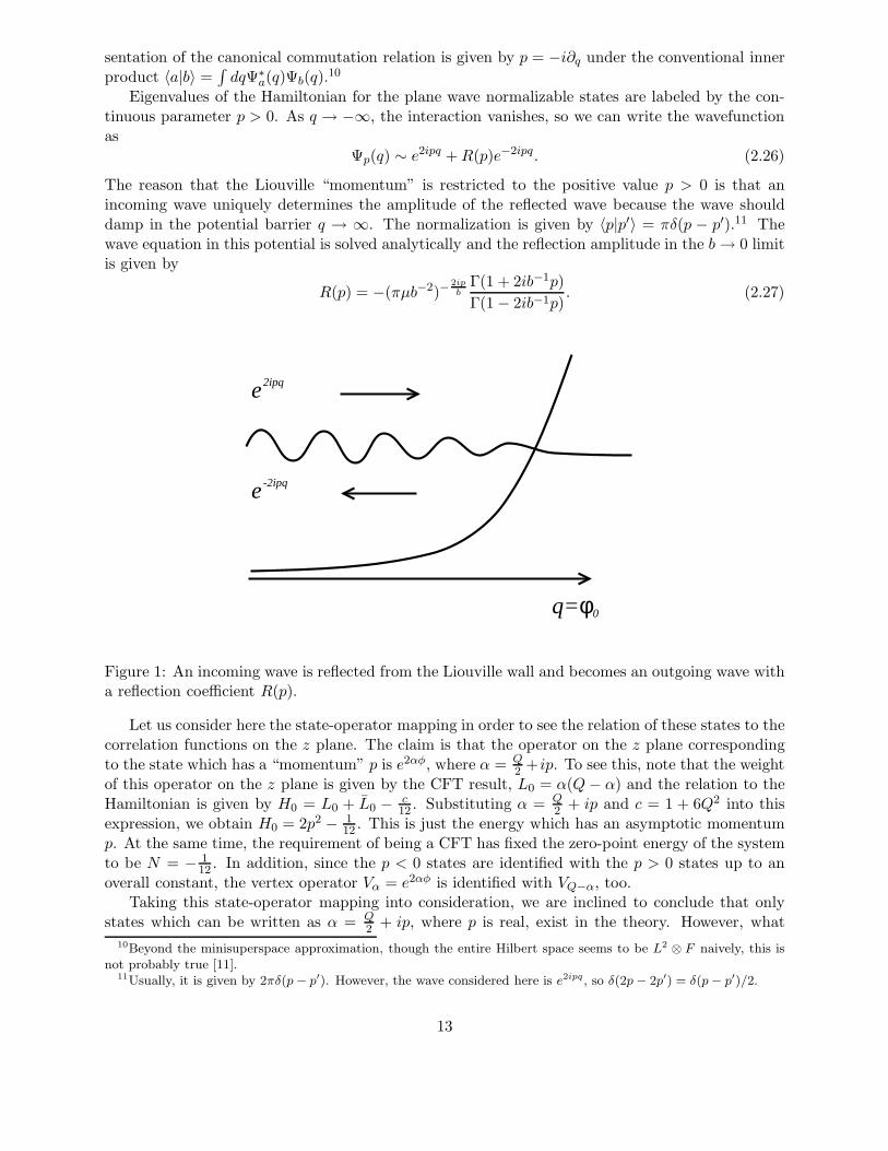
Eigenvalues of the Hamiltonian for the plane wave normalizable states are labeled by the con-tinuous parameter p > 0. As q → −∞, the interaction vanishes, so we can write the wavefunctionas
Ψp(q) ∼ e2ipq +R(p)e−2ipq. (2.26)
The reason that the Liouville “momentum” is restricted to the positive value p > 0 is that anincoming wave uniquely determines the amplitude of the reflected wave because the wave shoulddamp in the potential barrier q → ∞. The normalization is given by 〈p|p′〉 = πδ(p − p′).11 Thewave equation in this potential is solved analytically and the reflection amplitude in the b→ 0 limitis given by
R(p) = −(πµb−2)−2ipb
Γ(1 + 2ib−1p)
Γ(1 − 2ib−1p). (2.27)
e -2ipq
e2ipq
q=φ0
Figure 1: An incoming wave is reflected from the Liouville wall and becomes an outgoing wave witha reflection coefficient R(p).
Let us consider here the state-operator mapping in order to see the relation of these states to thecorrelation functions on the z plane. The claim is that the operator on the z plane correspondingto the state which has a “momentum” p is e2αφ, where α = Q
2 +ip. To see this, note that the weightof this operator on the z plane is given by the CFT result, L0 = α(Q− α) and the relation to theHamiltonian is given by H0 = L0 + L0 − c
12 . Substituting α = Q2 + ip and c = 1 + 6Q2 into this
expression, we obtain H0 = 2p2 − 112 . This is just the energy which has an asymptotic momentum
p. At the same time, the requirement of being a CFT has fixed the zero-point energy of the systemto be N = − 1
12 . In addition, since the p < 0 states are identified with the p > 0 states up to anoverall constant, the vertex operator Vα = e2αφ is identified with VQ−α, too.
Taking this state-operator mapping into consideration, we are inclined to conclude that onlystates which can be written as α = Q
2 + ip, where p is real, exist in the theory. However, what
10Beyond the minisuperspace approximation, though the entire Hilbert space seems to be L2 ⊗ F naively, this isnot probably true [11].
11Usually, it is given by 2πδ(p− p′). However, the wave considered here is e2ipq , so δ(2p− 2p′) = δ(p− p′)/2.
13

happened to the cosmological constant operator e2bφ, for instance? Is it not included in the theory?This is the very peculiar point in the state-operator mapping in the Liouville theory. Generally,the state corresponding to the operator e2αφ, even if α is real, is believed to exist but consideredas nonnormalizable one. Nonnormalizable as it is, there is a difficulty concerning the completenessof the states for example, but introducing the cut-off into φ removes some of the difficulties. In theminisuperspace approximation, this is equivalent to considering the wavefunction which formally hasan imaginary momentum. However, we do not allow every imaginary momentum state. Taking intoaccount that the asymptotic form of the wavefunction in the q → −∞ limit should be dominatedby e2ipq, the condition Re(α) ≤ Q
2 is required. This is what is called the Seiberg bound [1].Seiberg [1] has named the normalizable states (operators) as nonlocal and the nonnormalizable
states (operators) as local. The root of this naming is the behavior of the world sheet metric (e2bφ)under the inserted source in the WKB (semiclassical) approximation as we will see in the following.In fact, the source corresponding to the nonnormalizable states can be seen as the local curvaturesingularity from the world sheet point of view.
Leaving the canonical quantization, we next try to carry out the path integration by the WKB(semiclassical) approximation to calculate the Liouville correlation functions. The semiclassicallimit corresponds to the b → 0 limit. Before doing this, let us first consider the Ward-Takahashi(WT) identity which can be applied to any n-point function. The definition of the n-point functionis
〈e2α1φe2α2φ · · · e2αNφ〉 =
∫Dφe2α1φe2α2φ · · · e2αNφe−S , (2.28)
where the action is given by
S =1
4π
∫d2z
√g(gab∂aφ∂bφ+QRφ+ 4πµe2bφ
). (2.29)
Shifting φ as φ → φ − log µ2b , we can remove the µ dependence in front of the Liouville poten-
tial completely because we have made the path integral measure invariant under the translationas we have considered in the last section. Then using the Gauss-Bonnet theorem which states14π
∫d2z
√gR = 2 − 2g, we obtain the following exact µ dependence of the correlation function on
the genus g Riemann surface
〈e2α1φe2α2φ · · · e2αNφ〉g ∝ µ(1−g)Q−∑ i αi
b , (2.30)
which is what is called the Knizhnik-Polyakov-Zamolodchikov (KPZ) scaling law [41].Interestingly, if we consider the Liouville theory as the string theory, the string coupling constant
gs is multiplied to the genus g correlation function as g2(g−1)s . However, looking at the way the
power of the string coupling constant enters into the amplitude, we observe that this is just thesame way in which the power of µQ/b does (without vertices). That is to say, the partition functionof the Liouville theory does not depend independently on gs and µ, but it actually depends onlyon the particular combination µ−2
r = g2sµ
−Q/b. In addition, the power of the µr is determined asµ2−2gr in the usual manner. 12
Returning back to the semiclassical calculation on the sphere, we try to find the classical solutionφcl of the equation of motion and substitute back into the integrand of the path integral so thatwe obtain the zeroth order approximation of the correlation functions. The classical equation ofmotion (or the saddle point equation) for 〈e2α1φe2α2φ · · · e2αNφ〉 is given by
2
π∂∂φ− 1
4πRQ− 2µbe2bφ +
∑
i
2αiδ(z − zi) = 0. (2.31)
12Although for g = 0, 1, log correction is needed as the partition function diverges.
14
To see the necessary condition of the existence of the real solution of this equation, we integratethis equation over the world sheet. Setting µ > 0 and applying the Gauss-Bonnet theorem, weobtain the following inequality,
Q−∑
i
αi < 0. (2.32)
Under this condition, we will obtain the real semiclassical solution. If we can solve the Liouvilleequation with source, substituting the solution into the action gives the semiclassical correlationfunctions. However, the actual calculation has been done only for the three-point function. Thecalculation is complicated and not so illuminating, so we just quote the result [37]. Setting αi = ηi/band 〈e2α1φe2α2φe2α3φ〉 = exp(−Sc(η1, η2, η3)/b
2), we find
Sc = −(∑
i
ηi − 1
)log(πµb2) − F (η1 + η2 + η3 − 1) − F (η1 + η2 − η3)−
− F (η2 + η3 − η1) − F (η3 + η1 − η2) + F (0) + F (2η1) + F (2η2) + F (2η3), (2.33)
where F (η) =∫ η1/2 log γ(x)dx. Since it is difficult to extract the physical intuition from this result,
let us see the effect of the local vertex insertion instead. In the mean time, we will see the root ofthe local operator and the semiclassical meaning of the Seiberg bound. The solution of the classicalLiouville equation around a vertex is easily found to be
e2bφ =1
πµb2ν2|z|2ν−2
(1 − |z|2ν)2 (2.34)
where µ > 0 and α = 1−ν2b . If we regard this as the Weyl factor of the metric, we can interpret
it as the conical curvature singularity at the insertion point, which is the reason why we call theoperator with real α local. Since the deficit angle of the singularity is πν, it is necessary to haveν ≥ 0 to represent the semiclassical geometry. From this, the semiclassical bound 1
2b ≥ α is derived.Since Q ∼ 1
b in the b → 0 limit where the WKB approximation is good, we find the semiclassical
interpretation of the Seiberg bound α ≤ Q2 .
To conclude this section, we would like to make some comments on the perturbative treatment ofthe “interaction” µe2bφ and perform the one-loop calculation of the partition function. As we haveseen above, the Liouville theory has an exact WT identity for the µ dependence of the correlationfunction, so the perturbation in µ does not make sense for general µ. However, it is believed thatwhen the power of µ becomes an integer, the perturbative treatment gives the correct answer.This is the assumption which appears throughout this review. As the simplest application of thisassumption, let us calculate the one-loop partition function of the c = 1 Liouville theory with acompactified target space whose radius is R.
The reason of the calculability of this partition function is that the power of µ just vanishes forthe torus partition function. Thus, from the previous assumption, we can deal with the Liouvillefield as if they were free.13 The partition function which we would like to obtain becomes
Z1 =
∫[dΥ]
∫DXDφDbDce−S0. (2.35)
Taking the conventional torus moduli as the fundamental region F , this partition function can becalculated as
Z1 = Vφ
∫
F
d2τ
2τ2|η(q)|4(2π√τ2)−1|η(q)|−2Z(R, τ), (2.36)
13To see this more explicitly, we first integrate over the zero mode of φ. Then the non-zero mode path integralbecomes simply free. The only contribution from the zero-mode is given by the Liouville volume.
15
where Vφ =∫dφe−µe
2bφ= − 1
2b log µ is the volume of the Liouville direction and q = e2πiτ . Themeasure of the moduli is from the Beltrami differential and the next |η(q)|4 is from the ghostoscillator. (2π
√τ2)
−1 is from the integration of the Liouville momentum and the final |η(q)|−2 comesfrom the oscillator of the Liouville mode. In addition, the partition function of the compactifiedboson Z(R, τ) is given by
Z(R, τ) = 2πR1
2π√τ2|η(q)|2
∞∑
m,n=−∞exp
(−πR
2|n−mτ |2τ2
). (2.37)
Combining all these, we find the oscillator contribution cancels with that of the ghost:
Z1 = VφR
4π
∫
F
d2τ
τ22
∑
m,n
exp
(−πR
2|n−mτ |2τ2
). (2.38)
The integration over τ can be carried out.14 Using the formula∫Fd2ττ22
= π3 , we obtain
Z1 = Vφ1
12
(R+
1
R
). (2.39)
Note that this expression is invariant under the T-duality R→ 1/R as expected. As we have seenfrom the zero-mode integration, it is appropriate to set Vφ = −1
2 log µ with an implicit cut-off.Therefore the final result becomes
Z1 = − 1
24
(R+
1
R
)log µ, (2.40)
which reproduces the matrix model result (3.97) as we will see later in the next section.
2.4 Rolling Tachyon: Sen’s Conjecture
In this section, we briefly review the connection between the world sheet description of the tachyoncondensation and the Liouville theory. In general non-BPS branes are unstable because of thetachyon living on them. Sen [43] has conjectured that, besides the unstable vacuum, another kindof vacuum solution exists in the full open string field theory which has the perturbative tachyon. Inthis “true” vacuum, there exist only the closed string degrees of freedom without any open stringexcitation, and the energy difference from the unstable vacuum is simply the energy difference ofthe decaying D-brane.
For simplicity, let us discuss this conjecture by taking the bosonic D25-brane for example. Wemainly concentrate on the world sheet description here, so we will not discuss the SFT (stringfield theory) approach much in detail. However, let us in advance point out the major problem ofconsidering the time evolution of the tachyon by using the off-shell effective potential. For instance,suppose that we would like to construct the tachyon effective action from the on-shell scatteringamplitudes (which are obtainable from the first quantized perturbative string theory). From thesimple calculation, we find that the tachyon effective action at the three point level may be writtenas
S =
∫d26x
[−1
2∂µφ∂
µφ+1
2φ2 +
go3φ3
](2.41)
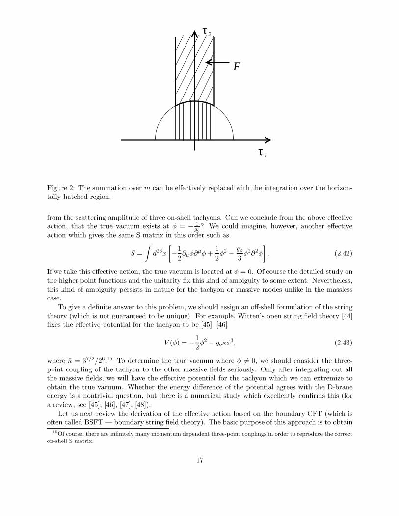
14The trick [42] is, instead of taking the summation over m, we can change the integration range of the moduli τfrom the fundamental region to the −1/2 ≤ τ1 < 1/2 region on the upper half plane τ2 > 0 (see figure 2). Then thecalculation is easily done. See appendix B.7.
16
τ 1
τ 2
F
Figure 2: The summation over m can be effectively replaced with the integration over the horizon-tally hatched region.
from the scattering amplitude of three on-shell tachyons. Can we conclude from the above effectiveaction, that the true vacuum exists at φ = − 1
go? We could imagine, however, another effective
action which gives the same S matrix in this order such as
S =
∫d26x
[−1
2∂µφ∂
µφ+1
2φ2 − go
3φ2∂2φ
]. (2.42)
If we take this effective action, the true vacuum is located at φ = 0. Of course the detailed study onthe higher point functions and the unitarity fix this kind of ambiguity to some extent. Nevertheless,this kind of ambiguity persists in nature for the tachyon or massive modes unlike in the masslesscase.
To give a definite answer to this problem, we should assign an off-shell formulation of the stringtheory (which is not guaranteed to be unique). For example, Witten’s open string field theory [44]fixes the effective potential for the tachyon to be [45], [46]
V (φ) = −1
2φ2 − goκφ
3, (2.43)
where κ = 37/2/26.15 To determine the true vacuum where φ 6= 0, we should consider the three-point coupling of the tachyon to the other massive fields seriously. Only after integrating out allthe massive fields, we will have the effective potential for the tachyon which we can extremize toobtain the true vacuum. Whether the energy difference of the potential agrees with the D-braneenergy is a nontrivial question, but there is a numerical study which excellently confirms this (fora review, see [45], [46], [47], [48]).
Let us next review the derivation of the effective action based on the boundary CFT (which isoften called BSFT — boundary string field theory). The basic purpose of this approach is to obtain
15Of course, there are infinitely many momentum dependent three-point couplings in order to reproduce the correcton-shell S matrix.
17

1g s
V(φ)
φ
Figure 3: Sen’s conjecture: the closed string vacuum is the global minimum of the effective tachyonpotential and the open string vacuum is the extremum of the potential. The potential differencecorresponds to the D-brane tension.
the effective action whose equation of motion yields the condition of vanishing beta functions forthe boundary perturbation on the world sheet. The claim [49] is as follows. When we write thepath integration on the disk as 〈 〉, the partition function with the tachyon and vector backgroundis given by
Z[T,A, ǫ] =
⟨e−∫dθ[
T (x)ǫ
+iAm(X)Xm]⟩
, (2.44)
where dot denotes a tangential differential and ǫ is introduced to imitate the Weyl scaling of themetric. This partition function is renormalizable by the power counting. Thus we should be ableto define the renormalized partition function as
Z[T (ǫ), A(ǫ), ǫ] = ZR[TR, AR]. (2.45)
Then the effective action [50, 51], [52, 53] is given by
S = ZR + βTδ
δTZR, (2.46)
where βT is the beta function for the tachyon.Performing the path integration around the static background and renormalization, we obtain
the final effective action
S =1
g
∫d26xe−T
√det(ηµν + 2πFµν)
[(1 + T )[1 +
1
2γµν∂µT∂νT ]
], (2.47)
where γµν =(
11+2πF
)µν. We have some comments on this effective action. First, since we have
expanded around T = const, we cannot trust this action for the on-shell S matrix while it is believed
18
to be exact as the effective potential of T . It is just accidental that this effective action properlyreproduces the three particle S matrix. Note that when T ∼ eikx, k2 = 1, all higher derivativeterms should contribute to the scattering amplitude. Similarly, though T = a+ uX2 is a solutionof the equation of motion at this order, this is just an artefact of the approximation.16
It is important to note that the extremum of this potential is located at T = ∞ and the energydifference from the perturbatively unstable vacuum is remarkably given by just the D-brane energy.In addition, if we consider the world sheet interpretation of the T = ∞ vacuum, this shows thatall the scattering amplitudes with boundaries on the world sheet becomes zero, which is naturallyinterpreted that after D-brane decays into the true vacuum, there are only closed strings and noopen string excitations in the theory.
As a complementary method to these off-shell effective action computations, there is anotheridea that we follow the time evolution of the decaying D-brane as the on-shell dynamics of thetachyon. For instance, we consider the boundary action
Shalf =
∫dθeX
0, (2.48)
or
Sfull =
∫dθ cosh(X0). (2.49)
It is known (after the Wick rotation of X0) that these are exactly marginal perturbations. 17 Sincethis interaction can be regarded as the time evolution of the rolling tachyon, it has been conjecturedthat the study of this theory leads to the understanding of the tachyon condensation. As we willsee in section 6.2, this theory is very similar to the boundary Liouville theory (in a sense it is an“analytic continuation”). Therefore the understanding of the Liouville theory is expected to resultin the understanding of the time evolution of the rolling tachyon.
The same notion can be applied not only to the open tachyon but also to the closed tachyon.However, the perturbation
Sfull? =
∫d2z cosh(2X0) (2.50)
is known to be not exactly marginal but marginally relevant [54] after we Wick rotate X0 and makeit sine-Gordon theory. As a result this tachyon profile does not become a CFT (= on-shell). Onthe other hand,
Shalf =
∫d2ze2X
0(2.51)
is conjectured to be exactly marginal. The relation between this perturbation and the Liouvilletheory will be discussed in section 6.2, but let us review the idea quickly. As has been discussedin the previous section, the noncritical string in d = 25 has formally b = i and there is no dilatonbackground because Q = 0. In addition, the cosmological constant can be seen as the tachyonbackground e2iφ. After Wick rotating φ as iφ = X0, we can interpret this system as the rollingtachyon system (2.51). Therefore, very formally, the analytic continuation b → i of the Liouvilletheory describes the tachyon dynamics of the critical bosonic string if we believe the Liouville theoryis analytic in b. The partial success and the problems are discussed in detail later in section 6.2.
16Because this solution makes X massive, it is not a marginal perturbation. Nevertheless we can extract a usefulinformation about the RG flow of the boundary field theory and obtain the effective action from this perturbation.This has been originally advocated in [50, 51].
17By the way, if these are really exactly marginal, they should be solutions of the BSFT equations of motion.However, even if we substitute this into the equation of motion, we should sum up all the higher derivative terms toconfirm this. Even if we had known all the higher derivative terms, it would not be necessary for the beta functionsto vanish, since the renormalization prescription could be different.
19

2.5 Ground Ring Structure
In this section, we discuss the BRST cohomology of the c = 1 Liouville theory with the EuclideanX boson. From the familiar discussion on the critical string theory (see also section 3.2.2), we havea massless tachyon vertex
Tq = cceiqX+(2−|q|)φ. (2.52)
At first sight, all other higher excitations are BRST exact with an experience in the critical stringtheory. However, the detailed study on the BRST cohomology reveals that this is not the case.For some special momenta, there exist BRST invariant physical discrete states (see e.g. [55, 56,57, 58, 59], [60, 61], [62], [63]). For a ghost number 1 sector (usual (1,1) vertex operators), we canconstruct them as follows. We prepare the special primary fields of the form
VJ,m(∂X, ∂2X · · · )e2miX(z) (2.53)
with conformal dimension J2. They form SU(2) multiplets with total spin J and Jz = m. Thenwe gravitationally dress them to obtain the dimension 1 operators as
VJ,m(z) = VJ,me2miX−2(J−1)φ(z). (2.54)
These are remnants of the longitudinal modes of the higher dimensional string theory, and as wewill see in the later section, they appear in the Euclidean scattering amplitudes as poles wheneverthe source momentum takes an integral value. This is because the OPE of two integer momentumtachyons is
einX−(−2+|n|)φ(z)e−inX−(−2+|n|)φ(0) ∼ 1
|z|2V|n|−1,0V|n|−1,0 + · · · . (2.55)
Actually, we have one more series of the BRST cohomology classes with ghost number 0 corre-sponding one to one to every VJ,m, which are discovered by Lian and Zuckerman. For example, atthe low excitation level, we have
O0,0 = 1O1/2,1/2 = (cb+ ∂φ+ i∂X)(cb+ ∂φ+ i∂X)eiX−φ
O1/2,−1/2 = (cb+ ∂φ− i∂X)(cb+ ∂φ− i∂X)e−iX−φ, (2.56)
which have dimension 0 and are BRST invariant. Furthermore we can show that ∂Oj,m are BRSTexact and hence the correlation function involving these states does not depend on their insertedpoints. Because of this property, we say these operators form a ground ring [60]. The OPE of theseoperators is given by the following form (modulo BRST exact terms)
Oj1,m1Oj2,m2 = Oj1+j2,m1+m2 (2.57)
if we have set the cosmological constat µ = 0. When we turn on the cosmological constant, thestructure itself remains the same, but the proportional factor changes somewhat. For example, wehave [16]
O1/2,1/2O1/2,−1/2 = µ. (2.58)
To derive this equality (with a precise numerical factor 1), we have to utilize the exact structureconstants of the Liouville OPE we will discuss in section 4, so we will not derive this relation here(see [16]. See also [64] for earlier study.).
20

Another important feature of the ground ring structure is that the tachyon vertex operatorsform a module under the action of the ground ring. If we take q > 0 in (2.52), we have
O1/2,1/2Tq = q2Tq+1
O1/2,−1/2Tq =µ
(q − 1)2Tq−1. (2.59)
On the other hand if we take q < 0, we have
O1/2,1/2Tq =µ
(q + 1)2Tq+1
O1/2,−1/2Tq = q2Tq−1. (2.60)
Though we will not discuss the ground ring structure any further, this ring structure is importantboth physically and mathematically. In the physical application, the ground ring shows a W∞algebra [61], [65], [66] and reveals an underlying integrable structure of the theory (which should beclosely related to the matrix model dual description). On the other hand, the geometrical pictureof the cohomology is beautifully exposed in [61], [59] particularly when we compactify X at theselfdual radius. The recent applications of the ground ring to the Liouville theory and the matrixmodel dual can be found in [16], [67].
2.6 Open-Closed Duality
In this section, we review the basic facts and ideas of the open/closed duality. Since this realm isso vast, we refer to other excellent reviews [68], [69], lecture notes (to name a few [70], [71], [72])or original papers [73], [74], [75] on this subject for details.
The first idea of the open closed duality is very old. Consider a long cylinder diagram of thestring theory. If we cut the diagram vertically, we obtain the cross-section which looks like a closedstring. In fact, the cylinder diagram has a pole when the propagating momentum is on mass-shellof the closed string spectrum. Therefore, the open string knows the existence of the closed string.However, this is not a duality. It simply states that the open string theory includes the closedstring sector naturally.
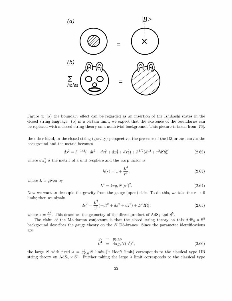
However, this observation makes it possible to write boundary conditions of the open stringtheory in the closed string language, which is just the boundary states or Ishibashi states. Let usconsider a world sheet with many holes. Formally, each hole can be represented by the closed stringboundary states.
VH =∑
n
cn(τ)On, (2.61)
where VH is the “hole operator” and On is the suitable basis of the boundary operators and cn(τ)is the moduli dependence (for large τ , c(τ) ∼ e−nτ ). We hope in some limiting case, the abovereplacement makes sense as a closed string theory after summing up all the hole contributions. Theproper limit is necessary, since the boundary states usually does not possess a normalizable normnor definite weight as the closed string states. The remaining world sheet theory is the closed stringtheory with modified backgrounds. Look at figure 4, where in the left side, the cat’s eyes, nose andmouth are holes where open strings have ends. After summing up those holes, we expect to obtainthe right side figure. Cat remains but grin disappeared.
The first and the most fundamental realization of the idea above is the Maldacena conjecture[73] of the AdS/CFT duality. We consider the N D3-branes in the flat type IIB background, onwhich we have the SU(N) N = 4 super Yang-Mills theory as the low energy effective theory. On
21
=
|B>
Σholes =
(a)
(b)
Figure 4: (a) the boundary effect can be regarded as an insertion of the Ishibashi states in theclosed string language. (b) in a certain limit, we expect that the existence of the boundaries canbe replaced with a closed string theory on a nontrivial background. This picture is taken from [76].
the other hand, in the closed string (gravity) perspective, the presence of the D3-branes curves thebackground and the metric becomes
ds2 = h−1/2(−dt2 + dx21 + dx2
2 + dx23) + h1/2(dr2 + r2dΩ2
5) (2.62)
where dΩ25 is the metric of a unit 5-sphere and the warp factor is
h(r) = 1 +L4
r4, (2.63)
where L is given byL4 = 4πgsN(α′)2. (2.64)
Now we want to decouple the gravity from the gauge (open) side. To do this, we take the r → 0limit; then we obtain
ds2 =L2
z2(−dt2 + d~x2 + dz2) + L2dΩ2
5, (2.65)
where z = L2
r . This describes the geometry of the direct product of AdS5 and S5.The claim of the Maldacena conjecture is that the closed string theory on this AdS5 × S5
background describes the gauge theory on the N D3-branes. Since the parameter identificationsare
gs = gYM2
L4 = 4πgsN(α′)2, (2.66)
the large N with fixed λ = g2YMN limit (’t Hooft limit) corresponds to the classical type IIB
string theory on AdS5 × S5. Further taking the large λ limit corresponds to the classical type
22
IIB supergravity on AdS5 × S5. Note that the symmetry of the both theories match, for theN = 4 super Yang-Mills theory actually has a superconformal symmetry which is isomorphic tothe (supersymmetric extension of the) AdS5 × S5 isometry group.
The Maldacena duality can be extended to other D-brane configurations – D-branes on conifoldor orbifold, wrapped branes around the cycles in the Calabi-Yau space etc. These gauge/gravitycorrespondence techniques have now become a strong tool to investigate the strongly coupled non-perturbative physics of the gauge theory.
Despite many efforts, however, the general proof of this duality along the line with the ideastated in the introductory part of this section is still missing. One of the major difficulties18 isthat the perturbative expansion of the small ’t Hooft coupling corresponds to the small radius limitwhere the world sheet description of the sigma model becomes ill-behaved. However, in the simplersetup, the open/closed duality has been proved.
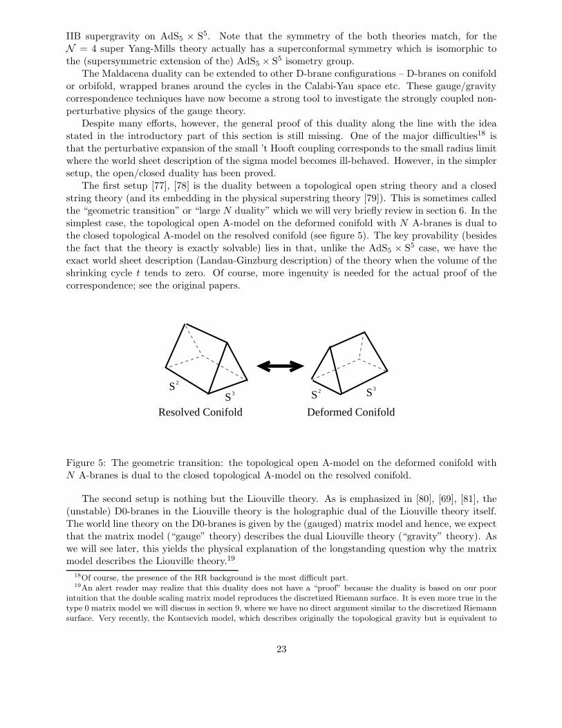
The first setup [77], [78] is the duality between a topological open string theory and a closedstring theory (and its embedding in the physical superstring theory [79]). This is sometimes calledthe “geometric transition” or “large N duality” which we will very briefly review in section 6. In thesimplest case, the topological open A-model on the deformed conifold with N A-branes is dual tothe closed topological A-model on the resolved conifold (see figure 5). The key provability (besidesthe fact that the theory is exactly solvable) lies in that, unlike the AdS5 × S5 case, we have theexact world sheet description (Landau-Ginzburg description) of the theory when the volume of theshrinking cycle t tends to zero. Of course, more ingenuity is needed for the actual proof of thecorrespondence; see the original papers.
S2
S2
S3 S3
Resolved Conifold Deformed Conifold
Figure 5: The geometric transition: the topological open A-model on the deformed conifold withN A-branes is dual to the closed topological A-model on the resolved conifold.
The second setup is nothing but the Liouville theory. As is emphasized in [80], [69], [81], the(unstable) D0-branes in the Liouville theory is the holographic dual of the Liouville theory itself.The world line theory on the D0-branes is given by the (gauged) matrix model and hence, we expectthat the matrix model (“gauge” theory) describes the dual Liouville theory (“gravity” theory). Aswe will see later, this yields the physical explanation of the longstanding question why the matrixmodel describes the Liouville theory.19
18Of course, the presence of the RR background is the most difficult part.19An alert reader may realize that this duality does not have a “proof” because the duality is based on our poor
intuition that the double scaling matrix model reproduces the discretized Riemann surface. It is even more true in thetype 0 matrix model we will discuss in section 9, where we have no direct argument similar to the discretized Riemannsurface. Very recently, the Kontsevich model, which describes originally the topological gravity but is equivalent to
23

To conclude this section, let us summarize what is important in the relation to the Liouvilletheory, some of which we would like to study further in the later section. The Liouville theoryis the simplest example of the open/closed duality. The dual description of the Liouville theory(which is the matrix theory) yields the nonperturbative information of the theory. Furthermore, itis interesting to note that the topological string duality is related to the c = 1 Liouville theory onthe selfdual circle. We will study this connection in section 6.3. It is very surprising that, after em-bedding the topological string duality into the physical superstring theory [83], the nonperturbativephysics of the N = 1 gauge theory is captured by the Liouville partition function.
2.7 Literature Guide for Section 2
The complete reference list for the earlier studies on the Liouville theory is beyond the scope ofthis review. We can find them in the earlier reviews such as [1], [7], [8], [6], [5], [4]. The reviewson the string field theory and the tachyon potential can be found in [45], [46], [47], [48]. For theAdS/CFT correspondence, [68] and [69] are the standard review articles.
3 Basic Facts 2: Matrix Model
In this section, we review the basic facts about the matrix model which is dual to the noncriticalstring theory (hence the Liouville theory). Good references are [7], [8], [6], [5], [84]. We mainlydiscuss the “physical” double scaling limit matrix model, and give only a few words on the “topo-logical” matrix models which actually yield the same information of the noncritical string theory.
The organization of this section is as follows. In section 3.1, we review the basic Hermitian onematrix model in the double scaling limit which describes the c < 1 noncritical string theory (theLiouville theory coupled to the minimal model). In subsection 3.1.1, we introduce the orthogonalpolynomial method to solve the theory and in subsection 3.1.2, we check the results from the WKBapproach. In subsection 3.1.3, we briefly discuss the integrable structure of the matrix models andtry to interpret all the c < 1 matrix models in a unified manner.
In section 3.2, we turn to the c = 1 matrix quantum mechanics. In subsection 3.2.1 we derivethe partition function of the theory, and in subsection 3.2.2, we discuss the tachyon scattering of thec = 1 noncritical string theory from various points of view and compare their results. In subsection3.2.3, we obtain the generating function of the tachyon S matrix which encodes all the scatteringphysics of the c = 1 matrix model (the Liouville theory coupled to a single boson).
3.1 c < 1 Matrix Model
In this section we solve the c < 1 string theory by the matrix model technique [85], [86], [87].We would like to define the noncritical string theory (2D gravity) as the continuum limit of
the random lattice. For simplicity, we first concentrate on the pure 2D gravity without matter(c = 0). The basic strategy is that we approximate the summation over all the metric by therandom triangulations of the world sheet.
Z ∼∫
Dg → limcont
∑
random triangulations
(3.1)
the physical two dimensional gravity, is reconsidered from the open string field theory perspective in [82]. They havegiven a world sheet proof of the duality between the Kontsevich model, which emerges from the open string fieldtheory and the closed topological (or physical) world sheet theory in line with the argument discussed in this section.
24

It is known that the right-hand side summation can be done efficiently by the matrix modeltechnique. Later in section 6, we will review the physical meaning of this matrix. Let us considerthe following matrix integral
eZ =
∫dM exp
[−N
(1
2trM2 +
κ
3!trM3
)], (3.2)
where M is an N ×N Hermitian matrix. It is well-known that when one expands this integral in1/N perturbatively, the expansion becomes the genus g expansion of the topology of each Feynmandiagram as follows
Z =∑
g
N2−2gZg(κ). (3.3)
We would like to connect each of this expansion with the genus expansion of the partitionfunction of the Liouville theory (2D gravity). Since the continuum limit seems to correspond tothe N → ∞ limit, we may conclude at first glance that the only genus 0 amplitude survives in thislimit. To avoid this difficulty, we take the κ→ κc limit at the same time, which is called the doublescaling limit, so that Zg(κ) diverges. It is known that the critical point κc does not depend on thegenus g. The way in which the partition function diverges is well-known and as we will see later,it is given by
Zg(κ) ∼ (κc − κ)(2−Γ)χ/2, (3.4)
where χ = 2−2g and Γ is called the string susceptibility whose value will be explicitly shown soon.Thus, in the double scaling limit, the matrix model perturbative expansion changes from the doubleparameter expansion of (1/N, κ) to the single parameter expansion of µr ≡ N(κ− κc)
(2−Γ)/2:
Z(µr) =∑
g
µ2−2gr fg. (3.5)
Considering that 1/N in the matrix model takes the role of the string coupling gs in the Liouvilletheory, this just corresponds to the fact that the actual expansion of the Liouville theory, contraryto the naive double expansion in gs and µ, is a single expansion of the particular combination ofgs and µ. The purpose of the following calculation is to find fg or its non-perturbative completionZ(µr) by using the matrix model technique.
(a) (b)
Figure 6: (a) the random triangulations of the Riemann surface can be done effectively by thematrix Feynman diagrammatic summation. (b) this nonplanar diagram corresponds to the genusone Riemann surface.
25
3.1.1 Orthogonal polynomial method
In the double scaling limit, we can solve this matrix model completely. In this subsection, wereview the solution which uses the orthogonal polynomials [88], [8], [7]. First, we diagonalize theHermitian matrix M : M = U †ΛU . Then we change the integration variable from M to a unitarymatrix U and diagonal elements λi, (i = 1 · · ·N). This can be done either by the Fadeev-Popovmethod or by the direct calculation. Here, we take the following step: set dU = dTU and introduceT , and the metric can be written as
trdM2 = tr(U †(dΛ + [Λ, dT ])U)2 = dΛ2 +∑
i,j
(λi − λj)2|dTij |2. (3.6)
From this expression, we can see that the independent elements of dM are dλi and the imaginaryand real part of the off-diagonal elements of dTij(i < j). Then the Jacobian of this transformationbecomes √
G =∏
i<j
(λi − λj)2 = ∆2(λ) = (detλj−1
i )2, (3.7)
which is the Vandermonde determinant. Substituting this transformation into the original integral,the dependence of T drops out completely. Consequently, the integral over T (or U integration)simply yields the trivial factor. Dividing this factor (“gauge freedom”), we obtain 20
eZ =
∫dλi∆
2(λ)e−V (λi). (3.8)
Note that the detail of the potential barely affects the final result in the double scaling limit as weare dealing with the critical behavior of the random lattice.21
Now let us introduce the orthogonal polynomials Pm(λ) as follows
∫ ∞
−∞dλe−V (λ)Pn(λ)Pm(λ) = hnδnm, (3.9)
where the polynomials start like Pn(λ) = λn + · · · . We can see from this
∆(λ) = detλj−1i = detPj−1(λi). (3.10)
When we substitute this expression of the Vandermonde determinant into the integral (3.8),the integration is easily done because of the orthogonality, which results in
eZ = N !N−1∏
i=0
hi = N !hN0
N−1∏
k=1
fN−kk , (3.11)
where fk ≡ hk/hk−1.In the double scaling limit, we take N → ∞. In this limit k/N can be regarded as a continuous
parameter 0 ≤ ξ ≤ 1. Also, fk/N can be regarded as a continuous function f(ξ). As a result, wecan write
1
N2Z ∼
∫ 1
0dξ(1 − ξ) log f(ξ). (3.12)
20Since there is a residual gauge freedom which corresponds to the Weyl group of U(N), further division by N ! isneeded in fact. However this does not change the following argument at all.
21When we use the symmetric potential, the resulting partition function is just double as that when we use thegeneric potential. Though the physical interpretation of this fact becomes important in the c = 1 matrix model, wedo not discuss it for the time being here.
26

In the following, in order to simplify the calculation, we take the symmetric potential V (λ) andlater we will divide the final result by 2 if needed. We notice that the following recursion relationfor the orthogonal polynomial holds
λPn = Pn+1 + rnPn−1, (3.13)
where rn does not depend on λ. The right-hand side does not have Pn term because the potentialis even. The lower terms also vanish owing to the orthogonality. Thus, we obtain
∫dλe−V PnλPn−1 = rnhn−1 = hn, (3.14)
which leads to fn = rn. Similarly, by the partial integration, we can derive
nhn =
∫dλe−V P ′
nλPn =
∫dλe−V P ′
nrnPn−1 = rn
∫dλe−V V ′PnPn−1. (3.15)
For concreteness, let us consider the following potential
V (λ) =1
2g
(λ2 +
λ4
N+ b
λ6
N2
), (3.16)
gV ′(λ) = λ+ 2λ3
N+ 3b
λ5
N2. (3.17)
We would like to obtain rn from this potential. First, we substitute (3.13) into the right-hand sideof (3.15). Substituting the same relation several times, we finally obtain the integrations which areproportional to hn−1, namely
∫e−V Pn−1Pn−1. Dividing this by hn−1, we have
gn = rn +2
Nrn(rn+1 + rn + rn−1) +
3b
N2(10 rrr terms). (3.18)
Then, taking the large N limit, we can write the above expression as
gξ = W (r) + 2r(ξ)(r(ξ + ǫ) + r(ξ − ǫ) − 2r(ξ))
= gc +1
2W ′′|r=rc(r(ξ) − rc)
2 + ǫ22rc(1 + 15brc)r′′(ξ) + · · · (3.19)
where ǫ = 1/N , W (r) ≡ r+ 6r2 + 30br3 and rc is the critical point of W (r). If we further tune thepotential and obtain the higher multi critical point, we have a double scaling limit which describesthe (m, 1) minimal model coupled to the two dimensional gravity.
It is important to note that, in the naive N → ∞ limit, (r−rc) ∼ (gc−gξ)1/2. Thus, comparisonof the 0 loop result22 with the above general argument (3.4) determines the string susceptibilityΓ = −1/2. Now, we take the following double scaling limit,
gc − g = gca2z
ǫ = 1/N = a5/2. (3.20)
where a → 0. In this limiting procedure, we fix µr = z5/4 = (g − gc)5/4N . Note this limit
is compatible with the general argument. For the actual calculation, it is convenient to changevariables such that gc − gξ = gca
2x and r(ξ) = rc(1 − au(x)). For the genus 0 amplitude, u2 ∼ x.
22 1N2Z =
∫ 1
0dξ(1 − ξ)(gc − gξ)1/2 = g
3/2c +
∫ 1
0dξ(gc − gξ)3/2 ∼ (gc − g)5/2.
27
With this change of variables (and rescaling of x), we obtain the following differential equation(Painleve I equation)
x = u2 − 1
3u′′. (3.21)
On the other hand, the partition function can be written in this limit as
Z =
∫ 1
0dξ(1 − ξ) log r(ξ) ∼
∫ z
a−2
dx(z − x)u(x). (3.22)
Differentiating this expression twice, we obtain
Z ′′(z) = −u(z). (3.23)
Therefore, if we know the solution of the Painleve I equation, the 2D quantum gravity is solved.The perturbative solution in powers of z−5/2 takes the form
u =√z(1 −
∞∑
k=1
ukz−5k/2), (3.24)
where uk are all positive. Note that this expansion is only asymptotic as we expect from the stringperturbation theory and the full solution has a one parameter ambiguity. The nonperturbative partof this expression will be further studied in section 6.6.
3.1.2 WKB method
In this subsection, we review the WKB (or steepest decent) method [89] to solve the large Nmatrix model. This may seem rather complicated and less efficient if we are only interested in thedouble scaling limit, but this method has a lot of applications including the recent Dijkgraaf-Vafaconjecture [90, 91, 92], [93, 94, 95]. For simplicity we consider here only the one-cut distribution ofthe eigenvalues which is sufficient for our application to the bosonic noncritical string theory.
Originally, we have to calculate the partition function,
eZ =1
N !
∫ N∏
i=1
dλie−N2Seff (λ), (3.25)
where the effective action is
Seff =1
N
N∑
i=1
V (λi) −1
N2
∑
i6=jlog |λi − λj|. (3.26)
In the WKB (large N steepest decent) approximation, we evaluate this by solving the equation ofmotion of the effective action and substituting back its solution into the partition function.
The equation of motion is
V ′(λi) =2
N
∑
j 6=i
1
λi − λj. (3.27)
In the large N limit, we can define the density of states:
ρ(λ) =1
N
N∑
i=1
δ(λ − λi) (3.28)
28
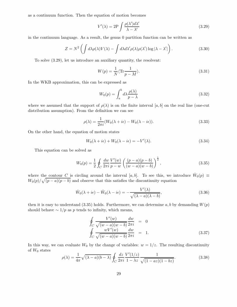
as a continuum function. Then the equation of motion becomes
V ′(λ) = 2P
∫ρ(λ′)dλ′
λ− λ′(3.29)
in the continuum language. As a result, the genus 0 partition function can be written as
Z = N2
(∫dλρ(λ)V (λ) −
∫dλdλ′ρ(λ)ρ(λ′) log |λ− λ′|
). (3.30)
To solve (3.29), let us introduce an auxiliary quantity, the resolvent:
W (p) =1
N〈Tr
1
p−M〉. (3.31)
In the WKB approximation, this can be expressed as
W0(p) =
∫ b
adλ
ρ(λ)
p− λ(3.32)
where we assumed that the support of ρ(λ) is on the finite interval [a, b] on the real line (one-cutdistribution assumption). From the definition we can see
ρ(λ) =1
2πi(W0(λ+ iǫ) −W0(λ− iǫ)). (3.33)
On the other hand, the equation of motion states
W0(λ+ iǫ) +W0(λ− iǫ) = −V ′(λ). (3.34)
This equation can be solved as
W0(p) =1
2
∮
C
dw
2πi
V ′(w)
p− w
((p − a)(p− b)
(w − a)(w − b)
) 12
, (3.35)
where the contour C is circling around the interval [a, b]. To see this, we introduce W0(p) ≡W0(p)/
√(p− a)(p − b) and observe that this satisfies the discontinuity equation
W0(λ+ iǫ) − W0(λ− iǫ) = − V ′(λ)√(λ− a)(λ− b)
, (3.36)
then it is easy to understand (3.35) holds. Furthermore, we can determine a, b by demanding W (p)should behave ∼ 1/p as p tends to infinity, which means,
∮
C
V ′(w)√(w − a)(w − b)
dw
2πi= 0
∮
C
wV ′(w)√(w − a)(w − b)
dw
2πi= 1. (3.37)
In this way, we can evaluate W0 by the change of variables: w = 1/z. The resulting discontinuityof W0 states
ρ(λ) =1
4π
√(λ− a)(b− λ)
∮
C
dz
2πi
V ′(1/z)1 − λz
1√(1 − az)(1 − bz)
. (3.38)
29
a b
CP C∞
Figure 7: The location of the cut and integration contours.
For example, take V = 12tTrM2. This leads to the famous Wigner distribution:
ρ(λ) =1
2πt
√4t− λ2. (3.39)
Next, we take the model V = 12TrM2 + gTrM4 which is relevant for the 2D gravity. In this
case, the location of the cut becomes
b = −a =
√1
6g
(−1 +
√1 + 48g
). (3.40)
Calculating the density of states, we obtain
ρ(λ) =1
π
(1
2+ ga2 + 2gλ2
)√a2 − λ2. (3.41)
Observing this solution, we notice that, for a general value of g, ρ(λ) ∼√a2 − λ2 around the edge
of the distribution a, but if we take g → gc = −1/48 then ρ(λ) ∼ (a2 −λ2)3/2 and this suggests thecritical behavior of g (double scaling limit will exist). To see this, we decompose the first term as2gπ
(14g + a2
2 + λ2), and demand 1
4g = −3a2
2 .
Finally, we can substitute this solution back into the effective action. Then the partition functionbecomes
Z0 = N2
(∫dλρ(λ)V (λ) −
∫dλdλ′ρ(λ)ρ(λ′) log(λ− λ′)
)
= N2
∫dλρ(λ)
(V (λ)
2− log |λ|
)
= N2
(1
24(a2/4 − 1)(9 − a2/4) − 1
2log(a2/4)
)
30
∼ N2(g − gc)5/2. (3.42)
Here, in the second line, we have used the following formula which can be obtained by integratingthe equation of motion,
V (λ) = 2
∫dλ′ρ(λ′)
(log |λ′ − λ| − log |λ′|
), (3.43)
where the integration constant is determined by demanding V (0) = 0. In the last line of (3.42), weactually mean
Z0 = c0 + c1(g − gc) + c2(g − gc)2 + c5/2(g − gc)
5/2 + · · · . (3.44)
The parts which have an integer power of (g − gc) do not show any singular behavior. Note thatthe absence of the term c1/2 and c3/2 is nontrivial. This partition function shows the same criticalbehavior as what we have obtained in the last subsection by using the orthogonal polynomialtechnique. Thus we have reproduced the genus 0 partition function by the WKB method as well.
We can also derive the formula (3.38) by using the loop equation. We concentrate on the one-cutmodel again. The loop equation is most easily derived from the WT identity of the matrix integral.
0 =
∫dMTr
(∂
∂M
)1
p−Mexp (−NTrV (M))
=
⟨(Tr
1
p−M
)2⟩
−N
⟨Tr
(1
p−MV ′(M)
)⟩. (3.45)
In the large N limit, the first term can be factorized as
⟨(Tr
1
p−M
)2⟩
=
⟨(Tr
1
p−M
)⟩2
= N2W0(p)2. (3.46)
We decompose the second term as follows,
⟨Tr
(1
p−MV ′(M)
)⟩=
⟨Tr
(1
p−M(V ′(M) − V ′(p) + V ′(p))
)⟩= NW0(p)V
′(p) +Nf(p),
(3.47)where f(p) is an (n− 1) degree polynomial of p which does not have a singularity.
Then the loop equation becomes in the large N limit
W0(p)2 = W0(p)V
′(p) + f(p), (3.48)
which can be solved as
W0 =1
2
(V ′ −
√(V ′)2 + 4f
). (3.49)
The single cut ansatz states that the above square root factorizes as
√(V ′(p))2 + 4f(p) = M(p)
√(p− a)(p − b) (3.50)
where M(p) is a regular function which does not have a singularity or cut. We have assumed a < bhere. This ansatz means that the eigenvalue density behaves like
ρ(λ) ∼M(λ)√
(a− λ)(λ− b), (3.51)
which can be regarded as a generalization of the Wigner distribution.
31

Now we can completely determine M(p) and hence W0(p) only with this information. SinceM(p) does not have a singularity except at p = ∞, the following relation holds,
M(p) =
∮
C∞
dw
2πi
M(w)
p− w=
∮
C∞
dw
2πi
V ′(w)
p− w
1√(w − a)(w − b)
, (3.52)
where the integral involving W (z) does not contribute because W (z) ∼ 1z as z → ∞ from its
definition. We can see this explicitly by the change of variable z = 1/w
M(p) =
∮
C0
dzV ′(1/z) − 2W0(1/z)
(1 − pz)√
(1 − az)(1 − bz)(3.53)
Substituting this expression into the loop equation, we obtain
W0(p) =1
2
(V ′(p) −
√(p − a)(p− b)
∮
C0
dzV ′(1/z)
(1 − pz)√
(1 − az)(1 − bz)
)(3.54)
We may note that the first term V ′(p) is just the residue at p = w. This observation leads to thefinal expression,
W0(p) =1
2
∮
C
dw
2πi
V ′(w)
p− w
((p− a)(p − b)
(w − a)(w − b)
)12
(3.55)
which is the same formula as above (3.35).
3.1.3 Integrable hierarchy
General c < 1 Liouville theory coupled to the minimal model reveals a very elegant structure whenwe see from the integrable hierarchy point of view. In this subsection we review only elementaryfacts following [7], [8] (see also [96]). For a complete description, we recommend the reader toconsult these reviews and original papers cited therein.
Let us begin with a one-matrix model and consider the possible generalization of the stringequation heuristically. For this purpose, we rescale orthogonal polynomials as
Πn(λ) = Pn(λ)/√hn (3.56)
so that the orthogonality condition simplifies as
∫ ∞
−∞dλe−V ΠnΠm = δnm. (3.57)
Then the recursion relation (3.13) can be rewritten as
λΠn =√rn+1Πn+1 +
√rnΠn−1
= QnmΠm. (3.58)
In the matrix notation, Q is symmetric: QT = Q, and hence becomes an Hermitian operator in thecontinuum limit. Indeed, in the multicritical model, it can be written as
Q = 2r1/2c +a2/m
√rc
(u+ rcκ2∂2x), (3.59)
32
where the first constant part is a non-universal term. It is convenient to introduce another matrixA by
∂
∂λΠn = AnmΠm, (3.60)
which satisfies[A,Q] = 1, (3.61)
by differentiating λΠ = QΠ with respect to λ. We define antisymmetric matrix P as
P =1
2(A−AT ), (3.62)
which also satisfies [P,Q] = 1. This can be easily seen if we notice A+AT = V ′(Q) which is derivedfrom 0 =
∫dλ ∂
∂λ(ΠnΠme−V ). In general if V is of order 2l, we have an order 2l − 1 differential
operator P in the continuum limit. The fundamental commutation relation [P,Q] = 1 is related tothe Lax representation of the KdV equations.
For the simplest example, we set l = 2 and Q = d2 − u. Then the third order anti-Hermitiandifferential operator P is given by P = d3 − 3
4u, d. Then the commutation relation yields
1 = [P,Q] =
(3
4u2 − 1
4u′′)′, (3.63)
which is equivalent to the Painleve I equation (3.21) with a trivial rescaling.In general, it can be shown [97] that the general differential operators satisfying [P,Q] = 1 yield
the string equation which includes the Liouville theory coupled to (p, q) minimal model. First, wetake Q as a qth order differential operator
Q = dq + vq−2(x), dq−2 + · · · + 2v0(x), (3.64)
where the constants vn correspond to various responses of the theory (e.g. vq−2 is the specific
heat). Then we define pth differential operator P as P = Qp/q+ , where Q1/q is a formally defined
pseudodifferential operator and the subscript + means that we take only the positive powers of d.In this way, we can in principle solve all the minimal models coupled to gravity. At the same time,the general theorem by [98] states that in general, P can be taken as
P =∑
k≥1
−(1 + k/q)tk+qQk/q+ , (3.65)
and physically the string equation following from [P,Q] = 1 corresponds to the minimal modelcoupled to gravity with the massive deformation. Since tn couples to the dual operators likeSint =
∫d2ztnOn, the derivative of the partition function with respect to tn yields the corresponding
correlation function. Also it is important to note that the dependence of the susceptibilities vn ontk is governed by the generalized KdV flow (see [8], [96] and references therein for a review onthis point). In a word, the partition function is given by the τ function of the generalized KdVhierarchy.
The integrable hierarchy of the double scaling limit of the (multi)matrix model is a good pointto relate them to the topological matrix model. It is known that the topological matrix model andthe physical double scaling matrix model yield the same integrable structure and hence the samephysical observables. The topological gravity aspect of the generalized KdV hierarchy is reviewedin e.g. [99], [100], [101], [102], [103]. See also [104], [105] for reviews on the integrable structure ofthe matrix models.
33

3.2 c = 1 Matrix Quantum Mechanics
In this section, we solve the c = 1 noncritical string theory (b = 1 Liouville theory) via the matrixquantum mechanics [6, 7].
3.2.1 Partition function
As in the last section, we consider the random triangulations of the world sheet. To obtain thec = 1 theory, we introduce free bosons on each lattice point. First, we consider the case where theboson is not compactified i.e. R = ∞. The partition function of the theory is given by
Z(g0, κ) =∑
g
g2(g−1)0
∑
Λ
κVV∏
i=1
∫dXi
∏
〈ij〉G(Xi −Xj). (3.66)
We suppose this yields the c = 1 noncritical string theory in the double scaling limit. While itis natural to take G(X) = e−
12X2
as the Polyakov action, it is known [106] that the precise formof the propagator does not matter in the double scaling limit. Thus we here take G(X) = e−|X|
for convenience. In fact, there exists a matrix model which reproduce this partition functionperturbatively. Let us consider the following matrix quantum mechanics
eZ =
∫DΦ(t) exp
[−N
∫ ∞
−∞dtTr
(1
2
(dΦ
dt
)2
+1
2Φ2 − κ
3!Φ3
)](3.67)
where, Φ is an N ×N Hermitian matrix and κ =√N/β. Evaluating this partition function by the
Feynman diagram expansion, we obtain
Z =∑
g
N2−2g∑
Λ
κVV∏
i=1
∫dXi
∏
〈ij〉e−|Xi−Xj | (3.68)
which is equivalent to (3.66) up to the propagator difference.Rewriting this path integral into the operator formalism of the quantum mechanics leads to the
following calculationeZ = lim
T→∞〈f |e−βHT |i〉, (3.69)
which means
limT→∞
Z
T= −βE0. (3.70)
Therefore, the evaluation of the partition function is equivalent to obtaining the lowest energyeigenvalue of this quantum system.
In order to know the energy eigenvalue, we canonically quantize this matrix quantum mechanics.As in the last section, we consider the diagonalization of the Hermitian matrix
Φ(t) = Ω†(t)Λ(t)Ω(t). (3.71)
The different point from the matrix integration considered in the last section is the appearance ofthe Ω(t) dependent part from the kinetic term:
TrΦ2 = TrΛ2 + Tr[Λ, ΩΩ†]2. (3.72)
34

To go further, we decompose ΩΩ† as follows
ΩΩ† =i√2
∑
i<j
Tijαij +
N∑
i
αiHi, (3.73)
where Tij is a nondiagonal generator of U(N) and Hi is a generator of the Cartan subalgebra. Sincethe Cartan part decouples from the action, these degrees of freedom are simply the gauge freedom.In other words, when we decompose an Hermitian matrix which has N2 degrees of freedom intoa unitary matrix which has N2 degrees of freedom and a diagonal matrix which has N degrees offreedom, there apparently exists a redundant part. Of course this is just the Cartan generator ofU(N).
Then we substitute this decomposition into the Lagrangian, and we find
L =∑
i
(1
2λ2i + U(λi)
)+
1
2
∑
i<j
(λi − λj)2α2
ij. (3.74)
To construct the Hamiltonian from this Lagrangian, we should be a little bit careful. Naive methodwould lead to a mistake just as it would lead to a mistake if we would try to obtain the Hamiltonianin the polar coordinate from the naive replacement pr → −i∂r etc. The important point is that thereis a Jacobian of the path integral measure which appears when we change the integration variables.We can obtain this Jacobian just as in the last section and it is given by DΦ = DΩ
∏i dλi∆
2(λ).The way to implement this Jacobian factor into the canonical quantization has been known
since the Pauli’s era. The gist is that we should write the Hamiltonian in terms of the generallycovariant Laplacian as in the case of the polar coordinate. The metric in this case is given by√G = ∆2(λ) as in the last section, so the kinetic term of the Hamiltonian is given by
− 1
2β2
1
∆2(λ)
d
dλi∆2(λ)
d
dλi(3.75)
in this coordinate.Taking the fact d2
dλ2i∆(λ) = 023 into consideration, we can rewrite this expression as
− 1
2β2∆(λ)
d2
dλ2i
∆(λ). (3.76)
Thus, the complete Hamiltonian finally becomes
H = − 1
2β2∆(λ)
d2
dλ2i
∆(λ) + U(λi) +Π2ij
(λi − λj)2, (3.77)
where Πij is the conjugate momentum of angular variable αij . Note that if we only need the lowestenergy state of this system, the wavefunction should possess a trivial dependence on the angularparameter because of the last term in the Hamiltonian, which means we can focus only on the trivialrepresentation of the U(N). On the other hand, when we consider the finite temperature situation,we may feel the necessity of including the contribution from the non-singlet representations at firstsight. In fact, however, we should discard these contributions for the calculation of the ordinary
23This expression must be totally antisymmetric with respect to λi, but only the Vandermonde determinant hasthis property. However, the degree of this expression does not match with that of the Vandermonde determinant, soit must vanish identically.
35
Liouville partition function as we will see.24 In any case, the singlet wavefunction is symmetricwith respect to the argument λi. Then we define a new “antisymmetric” wavefunction Ψ(λ) asΨ(λ) ≡ ∆(λ)χsym(λ). For this new wavefunction, the Schrodinger equation is given in a simpleform: (
− 1
2β2
d2
dλ2i
+ U(λi)
)Ψ(λ) = EΨ(λ). (3.78)
Since all the eigenvalues are diagonalized in this Hamiltonian, this is equivalent to the N inde-pendent fermions system with the potential U(λ). Note that the antisymmetry of the wavefunctionmakes the system fermionic. The lowest energy state is simply given by occupying the lowest Nstates with fermions, so the lowest energy becomes
E0 =N∑
i=1
ǫi, (3.79)
where ǫi is the energy of the ith excited state.For the actual calculation of this system, it is convenient to utilize the statistical mechanical
method. To begin with, we introduce the density of states as
ρ(ǫ) =1
β
∑
n
δ(ǫ− ǫn), (3.80)
Then we can write the total particle number and energy as
N
β=
∫ µF
−∞ρ(ǫ)dǫ
βE = β2
∫ µF
−∞ρ(ǫ)ǫdǫ, (3.81)
where µF is the Fermi energy under which the states are all occupied. Differentiating the firstequation and setting ∆ = π(κ2
c − Nβ ), we obtain
∂∆
∂µ= πρ(µF ). (3.82)
We can adjust the height of the potential freely to set the critical point to become µc = 0. Thenwe can write µ = −µF as a function of ∆. On the other hand, differentiating the second equationand leaving only the singular terms, we obtain
∂E
∂∆=
1
πβµ. (3.83)
In this way, the knowledge of ρ(ǫ) is enough to calculate the energy as a function of ∆ and β bysolving these equations. Since the noncritical string theory can be obtained in the double scalinglimit, we take N → ∞ and β → ∞ simultaneously. In this limit, the information of the detailedshape of the potential is almost lost and all we can see is the neighborhood around the critical point.Therefore there is no problem in approximating the potential with the inverted harmonic oscillator.Furthermore, for simplicity, we fill both sides of the potential with fermions (which corresponds totaking the even potential) and divide it by two at the end of the calculation.
24We will see the natural interpretation of this fact from the D-brane point of view later in section 6.
36

Taking the inverted harmonic oscillator as the Hamiltonian: h0 = 12p
2 − 12x
2, we can write thedensity of states as follows,
ρ(µ) = Trδ(h0 + βµ) =1
πIm Tr
[1
h0 + βµ− iǫ
]. (3.84)
The Green function for the harmonic oscillator was given by Feynman:
〈x| 112p
2 + 12ω
2x2 + βµ− iǫ|x〉 =
∫ ∞
0dTe−βµT
∫ x(T )=x
x(0)=xDx(t)e−
∫ T0dt 1
2(x2+ω2x2)
=
∫ ∞
0dTe−βµT
√ω
2π sinhωTe−ω[2x
2 coshωT−2x2]/2 sinhωT .
(3.85)
In this case, ω = −i, so it is convenient to “analytically continue” the Euclid time to the Minkowskitime i.e. T → iT 25.
Substituting this into the expression for the density of states, we obtain
∂ρ
∂(βµ)=
1
πIm
∫ ∞
0dTe−iβµT
T/2
sinh(T/2), (3.86)
after the x integration. Though this is a correct expression perturbatively in the µ−1 expansion, weshould interpret this result as one of the nonperturbative completions for the order e−βµ correction.Actually, it is known that the nonperturbative terms do depend on the precise form of the potentialfar from the critical point. For example, the third order potential, which is supposed to correspondto the bosonic noncritical string theory, is nonperturbatively unstable.
Expanding perturbatively in µ−1 and carrying out the integration over T , we obtain26
ρ(µ) =1
π
[− log µ+
∞∑
m=1
(22m−1 − 1)|B2m|m
(2βµ)−2m
]. (3.87)
The task left is to integrate (3.82) and express µ as the function of ∆. However, in hindsight,the final expression does not have a suitable ∆ expansion in the double scaling limit, rather µ0 isthe actual expansion parameter, which is defined as
∆ ≡ −µ0 log µ0. (3.88)
This special renormalization is related to the fact that c = 1 is the phase transition point of thenoncritical string theory 27. Accepting this ansatz, we find µ is given by
µ = µ0
[1 − 1
log µ0
∞∑
m=1
(22m−1 − 1)|B2m|
m(2m − 1)(2βµ0)
−2m + O(
1
log2 µ0
)], (3.89)
which can be confirmed by differentiating it directly. Integrating (3.83) next, we find
−βE =1
8π
[(2βµ0)
2 log µ0 −1
3log µ0 +
∞∑
m=1
(22m+1 − 1)|B2m+2|m(m+ 1)(2m + 1)
(2βµ0)−2m
]. (3.90)
25ω → −i is indeed an analytic continuation, but the transformation of T is actually not. Because of the iǫ term,this is not a analytic continuation but just a contour deformation, so the result does not change in this procedure.
26Note this is the expansion in terms of µ−1 not in µ. Since this is a nontrivial asymptotic expansion, we reviewthe details of the calculation in appendix B.3.
27In fact, there is a simple heuristic method for this calculation. ∂2Z(µr)
∂µ2r
= ρ(µr) holds. Note this is just the
Legendle transformation.
37

In the double scaling limit, we take the β → ∞ and µ → 0 limit while fixing βµ0 = µr. In thislimit, the sphere and torus contribution (logarithmically) diverges, which is also expected from thecontinuum Liouville analysis. Up to the zero-mode factor for X (and 1/2 for the bosonic string),this reproduces the correct partition functions for the sphere and the torus which are calculatedfrom the Liouville approach. We cannot calculate the comparable higher genus Liouville partitionfunction in the continuum approach yet.
Now we consider the case where the target space X is compact (with radius R). In this case,the matrix quantum mechanical expression becomes
eZR =
∫DΦ(t) exp
[−β∫ 2πR
0dtTr
(1
2
(dΦ
dt
)2
+ U(Φ)
)]. (3.91)
This can be rewritten in the operator formalism as
eZR = Tre−2πRβH , (3.92)
which describes the finite temperature system with the same Hamiltonian at R = ∞. Generallyspeaking, the calculation for the finite temperature system becomes more complicated than thezero-temperature case. However, if we limit ourselves in the singlet sector28, the calculation is notso difficult as it may seem.
First, we introduce the chemical potential as a convenient prescription to deal with the finitetemperature system in the N → ∞ limit:
N
β=
∫ ∞
−∞ρ(ǫ)dǫ
1
1 + e2πRβ(ǫ−µF ). (3.93)
Then, in the thermodynamical limit, the free energy (the string partition function) can be writtenas
∂ZR∂N
= µF . (3.94)
Setting the critical point of the potential to be zero: µc = 0, we obtain by differentiating the aboveequation,
∂∆
∂µ= πρ(µ) = π
∫ ∞
−∞deρ(e)
∂
∂µ
1
1 + e2πRβ(µ−e)∂ZR∂∆
=1
πβµ, (3.95)
where µ = −µc and e = −ǫ. The point is that only the density of states effectively receives somecorrections compared with the zero-temperature case.
Substituting the zero-temperature density of states ρ(e) into (3.95) and carrying out the inte-gration, we obtain
∂∆
∂µ= Re
∫ ∞
µ
dt
te−it
t/2βµ
sinh t/2βµ
t/2βµR
sinh(t/2βµR). (3.96)
Just as in the R = ∞ case, we introduce µ0 and perform the integration perturbatively. Aftersome algebra, the partition function is given by
Z =1
4
[(2βµ0
√R)2 log µ0 − 2f1(R) log µ0 +
∞∑
m=1
fm+1(R)
m(2m+ 1)(2βµ0
√R)−2m
], (3.97)
28As we will see in section 6, there is a physical ground which justifies this restriction. Practically, if we includethe non-singlet sector correction, undesirable properties such as the breakdown of the T-duality emerge [107].
38
where fn is a function of R+R−1 and manifestly invariant under the exchange of R and R−1. The
actual form is given by fm(R) = (2m−1)!∑m
k=0 |22k−2||22(m−k)−2| |B2k ||B2(m−k)|(2k)![(2(m−k)]!R
m−2k. This is the
celebrated Gross-Klebanov formula [108]. After we introduce µr = βµ0 and take the double scalinglimit (and divide it by two), we finally obtain the all-genus partition function of the compactifiedtwo dimensional noncritical string theory which reproduces the Liouville computation for the genuszero and one (see (2.37)).
Note that this expression is manifestly invariant under the following T-duality (up to diverginglog terms):
R → 1
Rµr → Rµr. (3.98)
The transformation of the string coupling constant is familiar, for the T-duality transforms thedilaton expectation value because of the one-loop correction. Finally, we explicitly calculate theR = 1 partition function where the radius is selfdual under the T-duality. This case is importantfor the application to the topological string as we will review in section 6.
Since ρ(µr) is given, we calculate the second derivative of the partition function via the conve-nient method based on the Legendle transformation
∂2Z
∂µ2r
= Re
∫ ∞
0
dt
te−iµrt
(t/2
sinh t/2
)2
. (3.99)
Carrying out the integration, we obtain
Z(µr) =1
2µ2r log µr −
1
12log µr +
∞∑
g=2
(−1)gB2g
2g(2g − 2)µ2−2gr . (3.100)
3.2.2 Tachyon scattering
Next we review the tachyon scattering in the two dimensional string theory. Since there are manygood review articles [6], [9], [7], [10] on the subject, the description here will be brief. In thefollowing, we derive the tachyon scattering amplitudes in three different but (should-be) equivalentways: the direct Liouville calculation, the direct matrix calculation and the collective field theoryof the Fermi surface.
Let us consider the on-shell vertex of the two dimensional (Liouville + time-like boson) stringtheory. After Wick rotating the X direction as X → it, the on-shell tachyon vertex is given by
V ±ω = e±iωt+iωφ+2φ, (3.101)
which has the weight (1, 1) as it should be. The minus sign corresponds to the incoming rightmoverand the plus sign corresponds to the outgoing leftmover. In the actual calculation, it is convenientto do in the Euclidean signature. This is done by
−iω → |q| (3.102)
so that the vertices become
V −ω → e−i|q|X+(2−|q|)φ
V +ω → e+i|q|X+(2−|q|)φ. (3.103)
39

These can be combined as Vq = eiqX+(2−|q|)φ, which represents the incoming wave when q < 0 andoutgoing wave when q > 0 respectively.29
The direct Liouville calculation is the most challenging program. We here consider the particularamplitude where the violation of the Liouville charge is an integer; then we analytically continuethe result [109], [110]. Of course, the calculation here is limited to the tree level amplitude.
The setup is the following. We consider the situation where one incoming wave is scatteredinto N outgoing waves whose (Euclidean) momenta are (q1, · · · , qN ) respectively. The simplestscattering occurs if we set the momentum of the incoming wave qN+1 to be 1 − N so that theLiouville momentum is conserved without any insertion of the Liouville potential. Here we havealso used the “energy” conservation:
∑N+1i=1 qi = 0.
Using the free field correlator, we can evaluate the N -point function explicitly. In addition, theintegration over the sphere can be carried out [111, 110]. The result is given by
〈Vq1Vq2 · · ·VqN+1〉 = lim
s→0
µs
2Γ(s)
πN−2
(N − 2)!
N∏
i=1
γ(1 − |qi|)
=πN−2
2
N∏
i=1
γ(1 − |qi|)Γ(1 − (N − 1))
Γ(N − 1)(N − 2)!
=(N − 2)!
2
N+1∏
i=1
γ(1 − |qi|)
= lims→0
1
2
N+1∏
i=1
γ(1 − |qi|)(∂
∂µ
)N−2
µs+N−2. (3.104)
Taking the appropriate decoupling limit, we can obtain the similar expression for non-zero (butinteger) s = 1 −N + |qN+1| with qi > 0, i = 1 · · ·N .
〈Vq1Vq2 · · ·VqN+1〉 =
1
2
N+1∏
i=1
γ(1 − |qi|)(∂
∂µ
)N−2
µs+N−2 (3.105)
This form has an obvious analytic continuation for non-integer s which is given by,
〈Vq1Vq2 · · ·VqN+1〉 =
1
2
N+1∏
i=1
γ(1 − |qi|)(∂
∂µ
)N−2
µs+N−2. (3.106)
In the above formula, the pole from the integer s should be renormalized as lims→0 µsΓ(s) =
log µ. In this case, we call the process as the “bulk scattering” because the scattering amplitudeis proportional to the Liouville volume. In this terminology, only the bulk scattering has beencalculated in the direct Liouville approach. The other amplitudes are conjectured by the analyticcontinuation.
We next consider the direct matrix model calculation. The natural object which correspondsto the tachyon vertex is given by the following puncture operator
P (q) ∼ liml→0
l−|q|O(q, l), (3.107)
where the loop operator O(q, l) is defined as
O(q, l) =
∫dxeiqxTre−lΦ(x). (3.108)
29Note that the normalization of the momentum here is somewhat different from what is used in the most of theother sections: qhere = 2pthere.
40

We can easily see that the insertion of this operator into the matrix model path integral correspondsto eliminating the loop of length l. We naturally expect the following correspondence
Vq ⇐⇒ P (q). (3.109)
The direct matrix model evaluation of the correlator is performed in the second quantized formalism,where we take the second quantized action as
S =
∫dλdxψ†
(− ∂
∂x+
∂2
∂λ2+λ2
4+ µ
)ψ. (3.110)
We rewrite the loop operator in this formalism as
O(q, l) =
∫dxeiqx
∫dλe−lλψ†ψ(x, λ). (3.111)
The calculation left is the application of the Wick theorem (at least in principle). The actualevaluation is highly technical, so we simply quote some of the lowest order results [7]30
〈P (q)P (k)〉 = −δ(q + k)Γ(1 − |q|)2µ|q|(
1
|q| + · · ·)
(3.112)
〈P (q1)P (q2)P (q3)〉 = δ(q1 + q2 + q3)
3∏
i=1
(Γ(1 − |qi|)µ|qi|/2
)( 1
µ+ · · ·
), (3.113)
where the omitted terms are the higher loop terms (which can be obtained explicitly in this formal-ism). Comparing these amplitudes with the previous direct Liouville calculation, we observe thatthe extra wavefunction renormalization factor 1
Γ(|q|) is needed to reproduce the amplitude. Hence,the exact correspondence is given by
T (q) =P (q)
Γ(|q|) , (3.114)
which is only confirmed at the tree level. However, the correspondence is believed to remain correctat the higher genus.
Finally, let us review the collective field method which is sometimes called the Das-Jevicki fieldtheory [112]. This can be obtained in various ways. Gross and Klebanov [113] have derived it fromthe bosonization of the non-relativistic fermion. Recall that the matrix model is equivalent to thenon-relativistic fermionic system whose second quantized Hamiltonian is given by
H =
∫dλ
[1
2∂λψ
†∂λψ − λ2
2ψ†ψ + µψ†ψ
]. (3.115)
First, we introduce new fermionic variables ΨL and ΨR as
ψ(λ, t) =eiµt√v(λ)
[e−i
∫ λ dλ′v(λ′)+iπ/4ΨL(λ, t) + ei∫ λ dλ′v(λ′)−iπ/4ΨR(λ, t)
], (3.116)
30Actually, there exists a very elegant graphical rule to calculate these matrix elements. We will briefly review themethod in the next subsection.
41

where v(λ) = dλdτ =
√λ2 − 2µ, which also determines a new variable τ in terms of λ. This makes
the Hamiltonian almost relativistic. Then we bosonize the chiral fermions as
ΨL(τ, t) =1√2π
: exp
[i√π
∫ τ
(ΠS − S′)dτ ′]
:
ΨR(τ, t) =1√2π
: exp
[i√π
∫ τ
(ΠS + S′)dτ ′]
:, (3.117)
where S is a massless bosonic field and ΠS is its canonical conjugate momentum. With thesevariables, the Hamiltonian is now
H =1
2
∫ ∞
0dτ
(Π2S + (S′)2 −
√π
2µ sinh2 τ
[ΠSS
′ΠS +1
3(S′)3
]+ tadpole
), (3.118)
where the tadpole term can be found in the literature [113], [6]. We can calculate the S matrix byusing this Hamiltonian. In this sense, S can be regarded as the space-time tachyon field (up to thewavefunction renormalization we will see later).
What is the physical meaning of the Hamiltonian? This can be clearly seen from the originalderivation of this collective Hamiltonian by Das and Jevicki [112], [9]. Going back to the originalmatrix Lagrangian:
L =1
2Tr(Φ2 + Φ2
), (3.119)
we introduce the collective density field as
φ(λ, t) =N∑
i=1
δ(λ − λi(t)). (3.120)
Then the action can be rewritten as follows
S =
∫dtdλ
[1
2
∂−1λ φ∂−1
λ φ
φ− π2
6φ3 + (−µ+
λ2
2)φ
]. (3.121)
In order to treat the tadpole term correctly, we consider the fluctuation around the classical solution
φ =1
π(v −
√π
v∂τS), (3.122)
where τ and v have already been introduced: v(λ) = dλdτ =
√λ2 − 2µ. Substituting this back into
the action (3.121), we rederive the bosonized action (3.118) up to the tadpole term which is relatedto the normal ordering and renormalization needed for the collective field theory to be finite. Thephysical interpretation of the collective field theory is now clear. The bosonic field S describes thesmall fluctuation of the Fermi surface (eigenvalue density).
We can use this Hamiltonian to calculate the scattering amplitude to any order of the pertur-bation. Instead of doing that, we would like to obtain the tree level (classical) scattering amplitudefollowing Polchinski [10] (see also [114]) by using the hidden symmetry of the theory (W∞ symme-try). Given the classical equation of motion
λ = p, p = λ, (3.123)
we have conserved quantities
v = (−λ− p)e−t, w = (−λ+ p)et. (3.124)
42
Furthermore, arbitrary powers of these are conserved31. Let us consider the following conservedquantity
vmn =
∫
F−F0
dpdx
2πvmwn, (3.125)
where F0 is the static Fermi surface. When t tends to −∞, the rightmoving fluctuation of theFermi surface is given by ǫ+(τ, t) = ǫ(t− τ) =
√π(ΠS − ∂τS).32 Evaluating the conserved quantity
in this limit, we obtainv → eτ−tǫ+(τ − t), w → 2e−τ+t. (3.126)
Similarly, in the t→ ∞ limit, we have
v → 2e−τ−t, w → eτ+tǫ−(τ + t), (3.127)
where ǫ−(τ, t) = ǫ(t + τ) =√π(−ΠS − ∂τS). In these variables, the conserved quantity can be
written as
vmn =2n
2π(m+ 1)
∫ ∞
−∞dte(n−m)(t−τ) ((ǫ+(t− τ))m+1 − µm+1
)
=2m
2π(n+ 1)
∫ ∞
−∞dte(n−m)(t+τ)
((ǫ−(t+ τ))n+1 − µn+1
)(3.128)
This expression enables us to calculate the tree level S matrix. To do this, we consider the modeexpansion of the incoming (outgoing) wave as
S(τ, t) =
∫ ∞
−∞
dk√8π2k2
[ake
−i|k|t+ikτ + a†kei|k|t−ikτ
](3.129)
where incoming k > 0 operators and outgoing k < 0 operators are not independent because ofthe Liouville wall. Substituting this into (3.128) with m = 0 and n = iω, we have the nonlinearexpression which reveals the relation between incoming modes and outgoing modes.
a†k = (1
2µ)−ik
∞∑
n=1
1
n!
(i√2πµ
)n−1 Γ(1 − ik)
Γ(2 − n− ik)∫ 0
−∞dk1 · · · dkn(a†k1 − ak1) · · · (a†kn
− akn)δ(±|k1| · · · ± |kn| − k), (3.130)
where ± sign in the delta function is related to whether we have chosen a creation operator oran annihilation operator in the braces before. Mode operators satisfy the canonical commutationrelation
[ak, a†k′ ] = 2π|k|δ(k − k′). (3.131)
Defining the in-states as
|k1 · · · kn : in〉 = a†k1 · · · a†kn|0〉, ki > 0, (3.132)
and similarly for the out-states, we can calculate the tree level S matrix using the canonical com-mutation relation (3.131). For example, the now familiar 1 → n amplitude is given by
〈k1 · · · kn; out|k; in〉 =
(i√2πµ
)n−1 Γ(1 + ik)
Γ(2 − n+ ik)2πδ(k1 + · · · + kn − k)
n∏
i=1
2πki. (3.133)
31If we define Cm,n ≡ vmwn, they constitute the generators ofW∞ algebra. We can easily see that Cm,n, Cm′,n′ =2(m′n− n′m)Cn+n′−1,m+m′−1 hold under the classical Poisson bracket.
32It is important to note that τ = − log(−λ) and ǫ± = ±(p± λ) in this limit. We will use this fact later in section6.
43

which agrees with the previous calculation if we further introduce the leg factor −i(µ)−ik2
Γ(ik)Γ(−ik) for
each external leg (for the Euclidean S matrix, this becomes −µ|q|/2 Γ(−|q|Γ(|q|) ). Note that this leg pole
factor is simply a pure phase in the Minkowski signature. Therefore this factor does not affect thecross-section unless we prepare the superposition states of the different momenta.
To see the origin of the leg factor, let us reconsider what we should expect as the external lineattached to the rest of the Feynman diagram in the collective field theory. Let us recall that thetachyon vertex corresponds to the puncture operator in the matrix model. Then, the correspondingoperator in the collective field theory becomes
O(l, q) =
∫dxeiqxTre−lΦ
=
∫dxeiqx
∫dλe−lλ∂τS
∂τ
∂λ
=
∫dxeiqx
∫dτe−lλ(τ)∂τS, (3.134)
where we have used the correspondence between the matrix model and the collective field theory:TrO(Φ) ∼
∫dλO(λ)S′(λ). We perform the Fourier transformation as O(l, q) = i
∫dkF (k, l)kS(q, k),
where
F (k, l) =
∫ ∞
−∞dτe−lλ(τ) cos(kτ)
S(x, τ) =
∫dqe−iqx
∫dk sin(kτ)S(q, k). (3.135)
Evaluating this with the classical motion λ(τ) =√
2µ cosh τ , we find
F (k, l) =π
2 sin(ikπ)
(I−ik(l
√2µ) − Iik(l
√2µ))
(3.136)
We need the small l limit of this function where we can replace it with
Iν(l√
2µ) → (l√
2µ/2)ν1
Γ(ν + 1). (3.137)
In calculating the Euclidean Feynman diagram, every external line should include this factor withthe propagator 1
q2+k2 and the momentum integration over k and q. We deform the k integration
in a special way [6]: for I−ik we pick up the pole at k = i|q|, while for Iik we pick up the pole atk = −i|q|. This seems strange but it is actually necessary in order to ensure the convergence of theintegral. Consequently we obtain the desired external leg factor
−(l√µ/2)|q|Γ(−|q|). (3.138)
Finally, we must not forget the additional leg factor needed to connect the matrix model punctureoperator with the Liouville vertex operator, T (q) = P (q)
Γ(|q|) . This completes the explanation of theleg factor in the collective field theory.
Let us summarize what we have learned in this (rather lengthy) subsection. There are threedifferent (but supposed to be equivalent) methods to calculate the tachyon scattering in the 2Dnoncritial string theory.
1. The direct Liouville calculation of the correlation functions of the vertex operators: this isconceptually straightforward but has only been performed for the tree level (special) ampli-tudes.
44
2. The direct matrix model calculation of the correlation functions of the puncture operatorswith the leg factor 1
Γ(|q|) : this provides the finite full genus answer, but the actual calculationis involved.
3. The collective field calculation of the S matrix for the massless S field with the leg factor−µ|q|/2 Γ(−|q|)
Γ(|q|) : S describes the fluctuation of the Fermi surface. However this method some-what hides the nonperturbative nature of the matrix model.
3.2.3 From MPR formula to DMP formula
In the last subsection, we studied how to calculate the tachyon S matrix from the matrix quantummechanical point of view. Actually, there is a very elegant graphical method to evaluate the tachyonS matrix even nonperturbatively. This has been done by Moore, Plesser and Ramgoolam (MPR)[115]. We briefly review their philosophy and the elegant and intuitive results without delving intothe detailed derivation.
The main claim is the following intuitive formula:
SCF = ιf→b SFF ιb→f , (3.139)
where ιf→b is the bosonization map and ιb→f is its inverse, and SFF is the S matrix for the freefermion (under the inverted harmonic oscillator potential). The tachyon S matrix is related to thecollective field S matrix SCF via multiplying the leg pole factors (see the last subsection). Theintuitive meaning of this formula is as follows. We first fermionize the incoming bosonic collectivefield by the asymptotic fermionization formula33
a(ω) →∫ ∞
−∞dξb(µ+ ξ)b†(µ− (ω − ξ)), (3.140)
where the incoming boson is normalized as [a(ω), a(ω′)] = ωδ(ω + ω′) and a†(ω) = a(−ω). Thenwe calculate the S matrix for the fermion. This is very easy since the fermion is free in thisrepresentation. Therefore the S matrix (just the reflection amplitude) is diagonal
bout(ω) = R(ω)bin(ω) = Sbin(ω)S−1, (3.141)
where
S = exp
[−∫ ∞
−∞dω logR(ω)b†in(ω)bin(ω)
]. (3.142)
Then we rebosonize again the scattered fermion, which yields the final state.Thus, the only nontrivial information needed to calculate the S matrix is the reflection amplitude
R(ω). This can be calculated by solving the quantum mechanical scattering problem. For example,the inverted harmonic oscillator which is restricted to the left side only34 has the following reflectionamplitude
R(ω) = µiωi
√1 + ie−π(µ+ω)
1 − ie−π(µ+ω)
√Γ(1
2 − i(µ+ ω))
Γ(12 + i(µ+ ω))
, (3.143)
33For the nonrelativistic fermion, bosonization-fermionization is only possible in the asymptotic region where bysuitable transformation we can treat them as if they were relativistic (see the last subsection), but for the S matrix,only the asymptotic region is necessary.
34This is the theory I in the language of [115]. In the modern sense, this theory is rather ad hook. We will seein part II of this review, how these stable (and unitary) theories emerge from the supersymmetric extension of theLiouville theory.
45

where we have omitted the irrelevant ω independent phase factor.The important corollary of the MPR formula (3.139) is that the collective S matrix is unitary
if and only if SFF is unitary and the bosonization map yields the complete set of states. Forexample, if we allow the tunneling amplitude which goes from the left-hand side of the potentialinto the right-hand side of the potential and only consider the left-hand side as the physical bosonicexcitation (theory II in the language of [115]), we have a non-unitary theory, which leads to theconclusion that the naive bosonic Liouville theory is not unitary nonperturbatively.
Let us go into the actual evaluation of the amplitude. There is a very intuitive diagrammaticrule to calculate the S matrix. We just list the rule (in the Minkowski signature for definiteness)here. To each incoming and outgoing boson, associate a vertex in the (t, τ) space. Connect pointsvia line segments to form a one-loop graph. Each line segment carries a momentum (energy) andan arrow. Once the line hits the “reflection line” the propagator is reflected as in figure 8 with thereflection factor R. These lines are joined according to the following rule:
1. Lines with positive (negative) momenta slope upwards to the right (left),
2. At any vertex arrows are conserved and momentum is conserved as time flows upwards. Inparticular momentum ωi is inserted at the vertex as in figure 8.
3. Outgoing vertices at (tout, τout) all have later times than incoming vertices (tin, τin): tout > tin.
To each graph we associate an amplitude, with reflection factors R and ± for upwards (down-wards) sloping direct propagators. Finally, we sum over graphs and integrate over kinematicallyallowed momenta, schematically
S = in∑
graph
±∫dω
∏
reflection
R(ω)R∗(−ω) (3.144)
For example, 1 → 2 scattering is represented by two diagrams (figure 9); then we have
S(ω → ω1 + ω2) =
∫ ω2
0dxR(ω − x)R∗(−x) −
∫ ω
ω1
dxR(ω − x)R∗(−x). (3.145)
In the actual evaluation, we can expand the reflection amplitude in the series of 1/µ as
R(ω) = 1 +∑
k
Qk(ω)
µk. (3.146)
Then we have the perturbative expansion of the S matrix to any desired order.Now that we have learned how to calculate any S matrix, let us consider the generating functional
of the tachyon amplitudes in the Liouville theory. First, we define the renormalized vertex operatoras
V ±ω =
Γ(−iω)
Γ(iω)µ1+iω/2V ±
ω , (3.147)
and define the following generating functional of the vertex correlators:
µ2F [t(ω), t(ω)] ≡⟨⟨e∫∞0 dωt(ω)V +
ω e∫∞0 dωt(ω)V −
ω
⟩⟩, (3.148)
where 〈〈· · · 〉〉 means a sum over genus and integration over the moduli space. On the other hand,the matrix model duality and the MPR formula suggest that the same generating functional canbe written as
µ2F [t(ω), t(ω)] = 〈0|eµ∫∞0 dωt(ω)α(−ω)Seµ
∫∞0 t(ω)α(ω)|0〉, (3.149)
46

R(-w1)*
R(w-w1)
-w
w
w1
w-w1
-w1
-w+w1
t
τ
Figure 8: The diagram for the MPR formula.
t
-w
-x
x-w
w-xw1
w2
x
w2-x
τ
-wx-w
-x τ
t
x
w1
w2
w1-x
w-x
0 ≤ x ≤ w2 w1 ≤ x ≤ w1+w2
Figure 9: The three body scattering calculation from the MPR formula.
47

where α(ω) is a bosonic creation operator and S is the fermionic S matrix (3.142). This conciseformula was first derived in [116] by Dijkgraaf, Moore and Plesser (DMP). Furthermore it has asimple compactified Euclidean analog. With a compactified radius β, we have
µ2F ≡⟨⟨e∑
n≥1 tnVn/β+∑
n≥1 tnV−n/β
⟩⟩
= − 1
β〈0|eiµ
∑n≥1 tnαnSeiµ
∑n≥1 tnα−n |0〉, (3.150)
where
S =: exp
(∑
m
logRpmψout−(m+1/2)ψ
outm+1/2
): (3.151)
and αn and ψn are related by the usual bosonization formula: ∂φ = ψψ.Now we take the special radius, namely the selfdual radius β = 1. Using the explicit expression
for R, we can show (see [116] for the derivation) that Z(t, t) = eF (t,t) is a τ -function of the Todahierarchy, satisfying an infinite set of constraints that form a W∞ algebra. Surprisingly theseconstraints can be integrated to another matrix model! We are not going into the derivation herebut just quote the final result [117].
We make use of the large N × N matrix A instead of tk whose relation is given by the Miwatransformation
tk =1
νkTrA−k, (3.152)
where ν = −iµ. Then the generating function is given by
Z(t, t) = eF (t,t) =
∫dM exp
[Tr
(−νM + (ν −N) logM − ν
∞∑
k=1
tk(MA−1)k
)]. (3.153)
This is what is called the W∞ matrix model. However we should note that this generating functiondoes not include the winding mode of the theory. It is not yet known how to implement them intothe matrix form.
3.3 Literature Guide for Section 3
In this section, we have provided only the minimal knowledge of the matrix model which is necessaryto follow the arguments in the later sections, and the complete reference list for the matrix modelis beyond the scope of this review. We can find the reference list of the matrix model in the reviewssuch as [7], [8], [6], [5], [84].
While in the main text, we have mainly discussed the physical matrix models, which are derivedfrom the discretization of the Riemann surface, there is another topological approach (the Kont-sevich model and the Penner model) to the noncritical string theory (topological matrix model).Surprisingly they give exactly the same result as the physical matrix models. The recent reviewon the topological matrix model and relation to the physical matrix model (emphasizing the c = 1R = 1 model) is [13]. The topological matrix model yields a discretization of the moduli space ofthe Riemann surface in a sense [118], [119], [120] as opposed to the Riemann surface itself, and itis a finite matrix model as opposed to the double scaling limit of the physical matrix model.
The connection between these two different perspective35 is curious and has caught a lot ofattention recently (e.g. [13], [122]). The former discusses the D-instanton physics which may
35Yet another formulation of c = 1 noncritical string theory has been given in [121], where they have used the“normal matrix” as a building block.
48
connect c = 1, R = 1 matrix model and the Penner model (or the W∞ matrix model). The latterproposes that the topological B model on CY3 is the right language to unify all these formulationsof the noncritical string theory (and others).
4 DOZZ Formula
In this section we derive the DOZZ formula [123], [37] and study its properties. The DOZZ formulais a proposal for the Liouville three-point function on the sphere which is the fundamental buildingblock of the Liouville theory as a CFT.
The organization of this section is as follows. In section 4.1, we review its original derivationby [37], where the analytic continuation of the perturbatively calculable amplitudes are utilized.In section 4.2, we study the reflection property of the DOZZ formula and its physical implication.In section 4.3, we rederive the DOZZ formula by using what is called Teschner’s trick [124], wherethe properties of degenerate operators are fully utilized. This trick will be repeatedly used in thisreview to derive many other Liouville amplitudes. In section 4.4, we review the higher equationsof motion as an application of the DOZZ formula, which may lead to the understanding of theintegrability of the minimal model coupled to the two dimensional gravity from the continuumLiouville perspective.
4.1 Original Derivation
Though the three-point functions (or the structure constants) in the Liouville theory have notbeen calculated from the first principle, there is a proposal by Dorn-Otto and Zamolodchikov-Zamolodchikov. We review their derivation and its properties in this section.
To begin with, we should note that for any CFT (on the sphere), the three-point function takesthe following general form
〈Vα1(z1)Vα2(z2)Vα3(z3)〉 = |z12|2∆12 |z23|2∆23 |z31|2∆31C(α1, α2, α3), (4.1)
where zij = zi − zj , ∆12 = ∆3 − ∆2 − ∆1 and ∆i is the weight of Vi.The claim of the DOZZ formula is
C(α1, α2, α3) =[πµγ(b2)b2−2b2
](Q−∑3
i=1 αi)/b
× Υ′(0)Υ(2α1)Υ(2α2)Υ(2α3)
Υ(α1 + α2 + α3 −Q)Υ(α1 + α2 − α3)Υ(α1 − α2 + α3)Υ(−α1 + α2 + α3), (4.2)
where Vα = e2αφ. We refer to appendix A.3 for the special functions such as Υ function. We usethe standard notation: γ(x) ≡ Γ(x)/Γ(1 − x). It may be just a trivial check, but note that thepower of µ satisfies the exact WT identity or the KPZ scaling law (2.30) .
The basic strategy to derive this three-point function is as follows. As we have seen in thelast section, the power of µ is determined from the exact WT identity for the general correlationfunctions in the Liouville theory. Thus, in general, the perturbation of µ is not reliable at all.However, if we adjust α or b properly, the power of µ becomes an integer, so there is a possibilitythat the perturbative calculation is valid. Here, we “assume” that the three-point function canbe calculated perturbatively when the power of µ becomes an integer.36 For the other part of
36This reminds us of the instanton calculation for the supersymmetric gauge theory (for reviews, see [125], [126]).In general, the naive instanton (not fractional) calculation does not yield the answer which satisfies the conditionsuggested by the symmetry argument, but in the particular situation where the symmetry argument and the nonva-
49

the parameter region, we will define it by the analytic continuation of s ≡ (Q −∑i αi)/b. Inthe actual calculation, we immediately observe the following basic fact. Since we calculate theperturbative Liouville theory by the Coulomb gas integral, the charge conservation yields the zero-mode divergence of the Liouville direction whenever the power of µ becomes an integer. We regardthis divergence as the pole of the analytically continued three point structure constant in terms ofs. This yields a very strict constraint on the analytic property of C(α1, α2, α3).
In order to study the actual structure of the poles, we try to obtain the three-point function byapplying the “perturbation theory”,
〈Vα1(z1)Vα2(z2)Vα3(z3)〉 =
∫Dφ
3∏
i=1
e2αiφ(zi)e−SL
∼∫
[Dφ]free
3∏
i=1
e2αiφ(zi)∞∑
n=0
(−µ)n
n!
(∫d2ze2bφ
)ne−SCG . (4.3)
We separate the zero mode of the path integration over φ(z) from the non-zero mode: φ(z) =φ0 + φ(z), and integrate over the zero mode first,
〈Vα1(z1)Vα2(z2)Vα3(z3)〉 ∼ −∞∑
n=0
(−µ)n
n!
1
2b(s− n)
∫[Dφ]free
3∏
i=1
e2αiφ(zi)
(∫d2ze2bφ
)ne−SCG .
(4.4)We assume this yields the pole structure of the Liouville three-point functions. We can calcu-
late the residue at s = n by using the formula for the correlation functions of the Coulomb gasrepresentation:
〈e2α1φ1 · · · e2αNφN 〉C.G;Q = δ
(Q−
∑
i
αi
)∏
i>j
|zij |−4αiαj (4.5)
after the elimination of the delta function (which becomes the pole instead). After a long calculation[127, 128] involving the nontrivial integration which we will not reproduce here (the final result issummarized in (A.14)), we obtain the residues of the correlator (4.4), calling it Gnα1,α2,α3
(z1, z2, z3),
Gnα1,α2,α3(z1, z2, z3) = |z12|2∆12 |z23|2∆23 |z31|2∆31In(α1, α2, α3) (4.6)
In(α1, α2, α3) =
( −πµγ(−b2)
)n ∏nj=1 γ(−jb2)∏n−1
k=0 γ(2α1b+ kb2)γ(2α2b+ kb2)γ(2α3b+ kb2), (4.7)
where∑3
i=1 αi = Q− nb.We would like to analytically continue this expression in s and determine C(α1, α2, α3). As we
will review later, this analytic continuation is unique if we demand the b→ b−1 duality [124]. Thuswe only check that the DOZZ formula actually satisfies this relation.
First, note that the residues satisfy the following functional relations,
In−1(α1 + b, α2, α3)
In(α1, α2, α3)= −γ(−b
2)
πµ
γ(b(2α1 + b))γ(2bα1)γ(b(α2 + α3 − α1 − b))
γ(b(α1 + α2 + α3 −Q))γ(b(α1 + α2 − α3))γ(b(α1 + α3 − α2)).
(4.8)
nishing instanton amplitude matches, the instanton calculation yields the exact answer. For other cases (in which wecannot use the naive instanton calculation), we can “analytically continue” the answer for the exact case because ofthe holomorphy of the theory.
50

To see this, we substitute the definition
(LHS) = −γ(−b2)
πµ
γ(2α1b+ nb2)γ(2α2b+ (n− 1)b2)γ(2α3 + (n− 1)b2)γ(2α1b)γ(2α1b+ b2)
γ(−nb2) ,
and use the relation γ(x) = 1/γ(1 − x).It is natural to assume that this functional relation holds for general s. The claim is
C(α1 + b, α2, α3)
C(α1, α2, α3)= −γ(−b
2)
πµ
γ(b(2α1 + b))γ(2bα1)γ(b(α2 + α3 − α1 − b))
γ(b(α1 + α2 + α3 −Q))γ(b(α1 + α2 − α3))γ(b(α1 + α3 − α2)).
(4.9)It is easy to see (4.2) satisfies this functional relation by using the difference formula of Υ function(A.59) which we have derived in appendix A.3. Furthermore, the fact that the DOZZ formula has apole at s = n follows immediately from the structure of the zeros of the Υ functions. Therefore, theDOZZ formula indeed satisfies the desired properties at the pole s = n which have been proposedby the perturbative calculation.
We have several comments on the DOZZ formula. As is remarked above on the uniqueness ofthe analytic continuation with respect to s, this formula has the following (quantum) symmetry,
b → b = b−1
µ → µ =(πµγ(b2))b
−2
πγ(b−2). (4.10)
This means that the DOZZ formula also has poles at
sb = Q− α1 − α2 − α3 = nb+mb−1, (4.11)
where Υ function indeed has a zero. This corresponds to the fact that the Liouville field theory hasdegenerate states besides V−nb/2, namely the dual series V−mb−1/2 as we will see in the alternativederivation of the DOZZ formula (what is called Teschner’s trick). In terms of the path integral, itcan be interpreted as follows. When we split the path integral measure Dφ(z) into the zero modeand non-zero mode, there should be a renormalization of the action which involves the Jacobianof the transformation (because the path integral is not free, this is nontrivial). We expect thisgenerates the “dual cosmological constant term37”
∆S =
∫d2zµe2bφ(z) (4.12)
However, this term violates the Seiberg bound as is discussed in section 2. Therefore some subtletiesexist when we include this term in the action.
On the other hand, this duality, with some further technical assumptions, enables us to provethe uniqueness (up to a constant multiplicity) of the solution of (4.9) [124].38 We sketch the proofhere.
The assumptions we need are the continuity of C with respect to α and the irrationality ofb2. Suppose we have another solution of the functional relation which we call D. If we define
37Since this does not actually contribute in the semi classical limit b → 0, it is appropriate to think of it as aquantum correction. Also, including this term in the action makes the above duality manifest. It is important to
note that the dual cosmological constant µ does not spoil the KPZ scaling law only if it scales as µb−2
.38Without this duality, there are actually infinitely many solutions of the functional relation. For instance, we can
take any function C(α) which is defined in the interval (0, b) and satisfies C(0) = C(b) = 0. Then we define the entireC(α) by the functional relation itself. These functions obviously satisfy the functional relation.
51
R = D/C, R has a period b and b−1 at the same time. However, when b2 is an irrational number,the function R must be a constant (which was first proven by Liouville himself! [129]). Thistheorem can be proven by the Fourier analysis. Thus the structure constant C is unique up to aconstant multiplication.
When b2 is a rational number, though this case has important applications such as a couplingto the minimal model, the above proof fails. We just assume the continuity of C with respect to band claim it to be unique for the time being. Besides, when c > 1, b being a complex number, thereexists a double periodic function in this case, so the derivation is completely invalid. As a specialcase, when c = 25, b becomes pure imaginary, and the above derivation becomes a little subtle andwe will reconsider it with special care later in section 6.
4.2 Reflection Amplitude
The DOZZ formula has the following remarkable reflection property:
C(Q− α1, α2, α3) = C(α1, α2, α3)S(iα1 − iQ/2), (4.13)
where S(P ) is what is called the “reflection amplitude”
S(P ) = −(πµγ(b2))−2iP/bΓ(1 + 2iP/b)Γ(1 + 2iP b)
Γ(1 − 2iP/b)Γ(1 − 2iP b). (4.14)
In the b→ 0 limit, this reproduces the result from the minisuperspace approximation (2.27).Let us discuss some physical implications of this result. The first thing to note is that we
can identify VQ−α with S(iα1 − iQ/2)Vα even quantum mechanically, which explains the quantumSeiberg bound. The second thing to note is that it is unitary when P is real in the sense thatS†S = 〈α|α〉〈α−Q|α−Q〉 = 1. Since S(P ) represents the scattering matrix of a particle from theLiouville wall, this should be so. Note the condition that P is real is needed to have a normalizablewave to test the scattering.
The last thing is the connection between the reflection amplitude and the spectrum (densityof states) of the theory. At first sight, there is no connection between them, so let us explainthis in the simpler quantum mechanics setup (see e.g. [130], [131]). Consider the one-dimensionalscattering problem from a potential U(x), where U(x) → ∞ as x→ ∞ and U(x) → 0 as x→ −∞.The energy eigenstate of this system can be written as follows (x→ −∞)
ψ(x) ∼ e2ipx + e−2ipx+iδ(p), (4.15)
where δ(p) is the phase shift of the outgoing wave with respect to the incoming wave. To relatethe phase shift to the density of states, we introduce a perfectly reflecting wall at x = −V . TheDirichlet boundary condition at x = −V quantizes the spectrum as
4pV + δ(p) = 2π
(n+
1
2
). (4.16)
In general situation, p and n are one-to-one, so we define the density of states as ρ = dndp . In this
setup, it becomes
ρ(p) =1
2π
(4V +
dδ(p)
dp
)(4.17)
This formula shows the connection between the phase shift (or the logarithm of the reflectionamplitude) and the density of states of the spectrum.
52

Now let us apply this formula to the Liouville reflection amplitude,
ρ(P ) =1
2π
(4V − 2
blog(πµγ(b2)) − i log
(Γ(1 + 2iP/b)Γ(1 + 2iP b)
Γ(1 − 2iP/b)Γ(1 − 2iP b)
)). (4.18)
At first sight, in the Liouville theory, it may seem that the volume is V ∼ 1/2b log µ and the firsttwo terms cancel out. However, as we will see, this is not the case. Rather, the volume factor makeslog µ→ log(µ/Λ) providing the cut-off.
Note that the density of states possess a nontrivial dependence on the Liouville momentum P .How is this fact consistent with the free path integral one-loop calculation done in section 2, wherewe have treated the density of states as if it did not depend on P? The answer is simple. When weonly consider the logµ dependent factor in the one-loop partition function, this does not make anydifference. The integration over the P dependent density of states simply yields a finite numberwhich can be absorbed into the cut-off log Λ.39 However, when we treat the tadpole cancellationetc, we must be careful about those finite parts. We will return to this issue later.
δ (p) e2ipq
e -2ipq+iδ
V
Figure 10: The reflection amplitude is related to the density of states.
4.3 Teschner’s Trick
In the following, we would like to rederive the DOZZ formula by what is called Teschner’s trick [124]which makes use of the degenerate representation of the Virasoro algebra in the Liouville theory.For this purpose, we can study the bulk degenerate states by the Kac formula [132], [133].40 TheKac formula states that the degenerate representation exists if and only if the weight of the highest
39At the same time, recall we have neglected the term log(∫d2ze2bφ) which can be obtained after the integration
over the zero-mode of φ. This may provide a certain number whose direct calculation seems impossible, whichcorresponds to the cut-off Λ
40Since the Liouville theory is not compact nor the degenerate operators are normalizable, some of the assumptionsneeded to derive the Kac formula are not satisfied. However the equation obtained in this way is consistent andcorrect a posteriori. This is close to the spirit of the Coulomb gas representation.
53

operator satisfies
∆rs =c− 1
24+
1
4(rα+ + sα−)2, (4.19)
where α± = 1√24
(√
1 − c±√
25 − c). For the Liouville theory, we have c = 1+6Q2 and Q = b+b−1.
For instance, setting (r, s) = (1, 2), we can immediately see V−b/2 is the degenerate representation.Similarly setting (r, s) = (1, 3), we obtain V−b. In general, we have a degenerate representation ifand only if α = −nb
2 − m2b , where (n,m) are positive integers. We can also derive the differential
equation which the degenerate representation satisfies. For (r, s) = (1, 2), this is written as
0 =
(L−2 −
3
2(2∆ + 1)L2−1
)φ21. (4.20)
In the Liouville theory, it becomes
(1
b2∂2 + T (z)
)V−b/2 = 0. (4.21)
For (r, s) = (1, 3), the differential equation is
0 =
[L−3 −
2
∆ + 2L−1L−2 +
1
(∆ + 1)(∆ + 2)L3−1
]φ31, (4.22)
and applying this to the Liouville theory we obtain
(1
2b2+ 2T (z)∂ + (1 + 2b2)∂T (z)
)V−b = 0. (4.23)
Note that although the equation for (1, 2) state might be obtained by using the semiclassicalequation of motion, the equation for (1, 3) state has an order b2 ambiguity of the operator orderingif we attempt to derive it from the equation of motion. This method which uses the degenerateconformal states removes this kind of ambiguity.
In order to derive the general three-point functions, we consider an auxiliary four-point functionfirst. Because of the conformal invariance, the four-point function essentially depends only on thecross-ratio:
z =z21z43z31z42
. (4.24)
Then the four-point function becomes
〈Vα4(z4)Vα3(z3)Vα2(z2)Vα1(z1)〉= |z42|−4∆2 |z41|2(∆3+∆2−∆1−∆4)|z43|2∆1+∆2−∆3−∆4)|z31|2(∆4−∆1−∆2−∆3)Gα4α3α2α1(z, z)(4.25)
This four-point function can be calculated either by first taking the OPE of (4, 3) and (1, 2) or bytaking the OPE of (1, 3) and (2, 4), which is the crossing symmetry. In terms of the three-pointfunction, this states
Gα4α3α2α1(z, z) =∑
α
C(α4, α3, α)C(Q− α,α2, α1)
∣∣∣∣Fs[α3 α2
α4 α1
]∣∣∣∣2
= |z|−4∆2Gα1α3α2α4(1/z, 1/z), (4.26)
where we implicitly set the Zamolodchikov metric of the vertex operator to be 〈Q− α|α〉 = 1.
54

In general we cannot solve this bootstrap equation because the number of the intermediatestates is infinite. The trick here is to set α2 = − b
2 so that it becomes a degenerate operator.Thanks to the differential equation derived above, the four-point function satisfies
(− 1
b2d2
dz2+
(1
z − 1+
1
z
)d
dz− ∆3
(z − 1)2− ∆1
z2+
∆3 + ∆2 + ∆1 − ∆4
z(z − 1)
)G(z, z) = 0, (4.27)
which means there are only two intermediate states in (4.26), α = α1 + sb/2, s = ±1. Furthermorethe differential equation determines Fs = Fα1+sb/2 in terms of the hypergeometric functions as
Fs(z) = zas(1 − z)βF (αs, βs, γs, z), (4.28)
where as = ∆α1+sb/2 − ∆2 − ∆1, β = ∆α3−b/2 − ∆3 − ∆2 and
αs = −sb(α1 −Q/2) + b(α3 + α4 − b) − 1/2βs = −sb(α1 −Q/2) + b(α3 − α4) + 1/2γs = 1 − sb(2α1 −Q). (4.29)
α 4 α 2 = -b/2
α 3 α 1
α 1 ± b/2
α 1α 3
α 4 α 2 = -b/2
=α 4 ± b/2
Figure 11: The conformal bootstrap enables us to obtain the functional relation for the three-pointfunctions.
To obtain the functional relation from the conformal bootstrap equation, we utilize the inversionformula of the hypergeometric function (A.47), which yields the following relation
Fs
[α3 α2
α4 α1
](z) = z−2∆2
∑
t=±BstFt
[α3 α2
α1 α4
](1/z). (4.30)
Substituting this relation into the crossing symmetry equation (4.26) and comparing the cross termsof the F+ and F ∗
−, which are absent in the right-hand side, we find the structure constant mustsatisfy
C(α4, α3, α1 + b/2)
C(α4, α3, α1 − b/2)= −C(α1,−b/2, Q− (α1 − b/2))
C(α1,−b/2, Q− (α1 + b/2))
B−+B−−B++B+−
. (4.31)
The right-hand side of this expression is actually calculable, as B’s are known from the inversionformula
B+− =Γ(γ+)Γ(β+ − α+)
Γ(β+)Γ(γ+ − α+)
55
B−− =Γ(γ−)Γ(β− − α−)
Γ(β−)Γ(γ− − α−)
B++ =Γ(γ+)Γ(α+ − β+)
Γ(α+)Γ(γ+ − β+)
B−+ =Γ(γ−)Γ(α− − β−)
Γ(α−)Γ(γ− − β−)(4.32)
and C in the right-hand side can be calculated by the perturbative Coulomb gas integral under theperturbative saturation assumption. First, C(α1,−b/2, Q − (α1 − b/2)) = 1 because this satisfiesthe conservation of the Liouville charge and we do not need any insertion of the Liouville potential.To calculate C(α1,−b/2, Q − (α1 + b/2)), we just need one insertion of the Liouville potential:
C(α1,−b/2, Q− (α1 + b/2)) = −µ⟨e2α1φ(1)e−bφ(0)e2(Q−α1−b/2)φ(∞)
∫d2ze2bφ(z)
⟩
Q,free
= −µ∫d2z|1 − z|−4α1b|z|2b2
= −πµ 1
γ(−b2)γ(2α1b)γ(2 + b2 − 2bα1).(4.33)
Substituting this and the actual form of B’s into the equation (4.31), we obtain the desiredfunctional relation for the structure constant after a little algebra,
C(α1 + b, α2, α3)
C(α1, α2, α3)= −γ(−b
2)
πµ
γ(b(2α1 + b))γ(2bα1)γ(b(α2 + α3 − α1 − b))
γ(b(α1 + α2 + α3 −Q))γ(b(α1 + α2 − α3))γ(b(α1 + α3 − α2)),
(4.34)where we have shifted α1. This is the same functional relation we have already derived in (4.9).The rest of the calculations to derive the DOZZ formula are the same and we will not repeat themhere.
By the way, note that we can redo the same reasoning above by replacing α2 = −b/2 withα2 = −1/(2b). In this way, we seem to obtain the second functional relation which determines thestructure constant uniquely. However this is not so automatic as it may seem. The point is if wereplace b→ b−1, we cannot calculate C(α1,−1/(2b), Q−(α1+1/(2b))) without a further assumption.Of course, the natural guess is that the quantum correction provides the dual cosmological constantterm ∆S =
∫d2zµe2bφ(z) in the functional integration as we have discussed above41, but this is
rather an assumption or a conjecture. Therefore Teschner’s trick suggests the b→ b−1 duality of theLiouville theory, but does not prove it. Alternatively saying, to fix the ambiguity of the quantization,we should demand this duality to define the quantum Liouville theory. However, the generalLiouville bootstrap suggests that the DOZZ formula is compatible with the CFT requirement,so perhaps the duality symmetry is the fundamental requirement for the Liouville theory to beconsistent as a CFT. The nature of the duality in the Liouville theory has been further studied in[134], [135] and [136].
4.4 Higher Equations of Motion
As an application of the DOZZ formula, we review the higher equations of motion in the Liouvilletheory, which is proposed in [137]. The rough idea can be seen from the simplest Liouville equationof motion. The Liouville equation of motion is given by
∂∂φ = πbµe2bφ. (4.35)
41It is interesting to note that µe2bφ = µS(b)e2b−1φ = µb2e2b−1φ.
56

As a result, the derivative of any correlation function with respect to the cosmological constantbecomes
∂
∂µ〈U1 · · ·Un〉 =
−1
πµb
∫d2z〈U1 · · ·Un∂∂φ(z)〉. (4.36)
The integration over d2z turns to the boundary integration which results in the KPZ scaling relation:
∂
∂µ〈U1 · · ·Un〉 = −
∑i αi − (1 − g)Q
µb〈U1 · · ·Un〉. (4.37)
The purpose of this section is to obtain the higher derivative counterparts of the above argument.To begin with, let us introduce the logarithmic degenerate field as
V ′α =
1
2
∂
∂αVα = φe2αφ, (4.38)
and we take α as the degenerate representations: V ′mn = V ′
α|α=αmn . The first proposition [137] isthatDm,nDm,nV
′m,n is a primary field. HereDm,n denotes the differential operator which annihilates
the degenerate primary operator Vm,n (like in (4.21) and (4.23)).The proof of this proposition is as follows. Consider Dm,nVα in the vicinity of α = αm,n. From
the analyticity in α, we have Dm,nVα = (α − αm,n)Am,n + O((α − αm,n)2), where Am,n is an
operator of dimension (∆m,n,∆m,n +mn) which is no more right primary but still a left primarywith the same dimension of the degenerate operator.42 Because of the degenerate dimension,Dm,nAm,n = 2Dm,nDm,nV
′m,n is also a left primary. Since we could inverse the roles of Dm,n and
Dm,n, Dm,nDm,nV′m,n is a primary field of dimension (∆m,n +mn,∆m,n +mn). That is to say
Dm,nDm,nV′m,n = Bm,nVαm,n , (4.39)
where αm,n = −(m− 1)b−1/2 + (n + 1)b/2. Bm,n can be calculated from the DOZZ formula (4.2)by applying (4.39) to the three-point function. The direct calculation shows that it is given by
Bm,n =(πµγ(b2)b2−2b2
)n Υ′(2αm,n)Υ(2αm,n)
=(πµγ(b2)
)nb1+2n−2mγ(m− nb2)
n−1,m−1∏
k=1−n,l=1−m,(k,l)6=(0,0)
(lb−1 + kb) (4.40)
As a possible application of this formula, [137] has considered the two dimensional minimalgravity theory. The (p, q) minimal model has a central charge
cM = 1 − 6(b−1 − b)2, (4.41)
where b =√p/q and the same b is used for the Liouville part. The matter primary field Φm,n has
a conformal dimension∆Mm,n = 1 − ∆m,n −mn. (4.42)
Thus the gravitationally dressed (1, 1) primary fields are given by
Um,n = ΦMm,nVm,n, (4.43)
42We have a different left and right notation from [137]. The left primary which has the same dimension as thedegenerate operator may seem to vanish, as in the rational conformal theory, when we act Dm,n, but this is not thecase here. It remains to be a nonvanishing left primary field. The same thing happens in the boundary operator suchas B− b
2
as we will see in the next section.
57

where Vm,n = Vαm,n is the operator which appears in the higher equations of motion (4.39). Fur-thermore, since ΦM
m,n is the degenerate field, DMm,nΦ
Mm,n = DM
m,nΦMm,n = 0. If we define the joint
operators Dmn asDm,n = Dm,n −DM
m,n, (4.44)
we finally have the following identity for the correlation function in the minimal gravity,∫d2z〈Um,n(z) · · · 〉MG =
1
Bm,n
∫d2z〈Dm,nDm,nΘ
′m,n(z) · · · 〉MG, (4.45)
where Θ′m,n = ΦM
m,nV′m,n and the subscript MG stands for the path integration over the minimal
model, the Liouville field and the conformal ghost.The further conjecture by [137] is that Dm,nDm,nΘ
′m,n(z) is actually BRST exact up to the total
derivative:Dm,nDm,nΘ
′m,n(z) = ∂∂(Hm,nHm,nΘ
′m,n) + BRST exact, (4.46)
where Hm,n are operators of level mn−1 with ghost number 0 constructed from Ln, LMn and ghosts
(see e.g. [62] for explicit construction).If this conjecture is true, the evaluation of any BRST closed correlation function and its in-
tegration over the moduli space is reduced to the boundary terms. However, we expect that thisis the case from the matrix model integrability of the minimal gravity. Indeed, the equivalence ofthe physical matrix model and the topological gravity states that the integration of BRST closedcorrelation functions over the moduli space should be reduced to the cohomological integration.We expect that this observation and higher equations of motion play significant roles in provingthe integrability of the minimal gravity from the continuum Liouville approach. This has not yetbeen done, but it is an important problem and we hope it will be solved in the near future.
4.5 Literature Guide for Section 4
For a general review of the subjects discussed in this section, we recommend an excellent review[11]. In this section and the followings, we assume the basic knowledge about the conformal fieldtheory. For the standard references of the CFT, we refer to [138], [139] and [140].
The original proposal of the DOZZ formula has been given independently in [123], [37]. In themain text, we have not done consistency checks, but of course, we have many supporting checksof the proposal in the literature. Besides the original checks done in [37], where the semiclassicallimit (see also [141]) and the numerical conformal bootstrap are discussed, consistency checks withthe general fusion and braiding property of the chiral part of the Liouville operators proposed byGervais and his collaborators [142, 143, 144, 145, 146, 147] have been done (those authors haveused the similar technique to Teschner’s trick). The perturbative check of the DOZZ formula canbe found in [148] by applying the method in [149]. For the canonical quantization approach, see[150, 151].
With these developments, the consistency of the DOZZ formula as a CFT is finally given (witha mild assumption) by proving the general conformal bootstrap in [152], which is reviewed in [11],[153] and [12]. This is important because at least we have a nontrivial irrational CFT defined bythe DOZZ formula irrespective of whether or not the CFT is actually describing the quantizationof the Liouville action. Unfortunately, we have not been able to discuss this issue in the main text,so an interested reader should consult these papers.
The higher equations of motion and possible application to the Liouville theory coupled to theminimal model is proposed in [137]. The logarithmic behavior is also observed in [154]. We expectthat this observation is the first important step to prove the integrability of the minimal gravity
58
from the continuum Liouville perspective. It may be possible in the near future that the integrationover the higher genus Liouville correlator dressing the minimal matter is explicitly reduced to thetopological gravity without a help of the matrix model.
5 Boundary Liouville Theory
In this section, we discuss the boundary Liouville theory. The Liouville theory admits two kinds ofboundary states, the FZZT (Fateev-Zamolodchikov-Zamolodchikov [2], Teschner [155]) brane andthe ZZ (Zamolodchikov-Zamolodchikov [3]) brane. They correspond to the brane extending in theLiouville direction and the one localized in the Liouville direction respectively. We review theirbasic properties here. The organization of this section is as follows.
In section 5.1, we discuss the FZZT brane. In subsection 5.1.1, we derive the one-point functionby the boundary bootstrap method. In subsection 5.1.2, we derive the boundary two-point function.In subsection 5.1.3, and subsection 5.1.4 we show the bulk-boundary structure constant and theboundary three-point function.
In section 5.2, we discuss the ZZ brane. In subsection 5.2.1, we derive the bulk one-pointfunction by the boundary bootstrap method as has been done in the FZZT brane. In subsection5.2.2, we present a unified way to view various boundary states from the modular bootstrap method,which also reveals the nature of the open strings propagating on these branes. In subsection 5.2.3we show the bulk-boundary structure constant.
5.1 FZZT Brane: D1-Brane
The FZZT brane is the brane which exists in the open sector of the Liouville theory [2], [155]. Thisbrane is extending in the Liouville direction, so we can think of it as a D1-brane on which the openstrings have the Neumann boundary condition (if we take c = 1 and regard X as time).
The starting point is the Liouville action for the open sector, namely on the world sheet withboundaries:
S =
∫
Γd2z
√g
(1
4πgab∂aφ∂bφ+
1
4πQRφ+ µe2bφ
)+
∫
∂Γdxg1/4
(QKφ
2π+ µBe
bφ
), (5.1)
where K is the extrinsic curvature on the boundary. Here, we discuss only the case of the disktopology. The boundary interaction ebφ is determined by the geometrical requirement from thepower of g1/4, and the coupling to K is uniquely fixed by the relationship between the perturbativeexpansion of the string interaction and the Euler number of the world sheet which can be countedby the Gauss-Bonnet theorem with boundaries:
1
4π
∫
Σ
√gR+
1
2π
∫
∂Σg1/4K = χ = 2 − 2g − h. (5.2)
In the actual calculation, it is convenient to take the upper half side of the complex plane as theworld sheet coordinate.
The primary fields which we would like to consider now are the bulk operator Vα = e2αφ and theboundary operator Bβ = eβφ. The central discussion below is to obtain the correlation functionsinvolving these. The conformal weight of the boundary primary operator Bβ is given by
∆β = β(Q− β). (5.3)
59
We can see this from the fact that the “charge conjugated operator” (which means it has a unitZamolodchikov metric with respect to the original one) BQ−β should have the same dimension asBβ and that its dimension should become ∆β = β2 when Q = 0.
Moreover, since the path integral measure is invariant under the change of variable: φ(z) →φ(z) − 1
2 log µ, the exact WT identity for the correlation functions holds,
〈Vα1 · · ·VαnBβ1 · · ·Bβm〉 = µ(Q−2∑
i αi−∑
j βj)/2bF
(µ2B
µ
). (5.4)
Note the power of µ, which was Q−∑i αi for the sphere, but now becomes Q−2∑
i αi−∑
j βj forthe disk. This is because the Gauss-Bonnet theorem requires the “charge” of Q to be proportionalto the world sheet Euler number.
Solving this boundary CFT amounts to determining the following correlation functions in prin-ciple.
1. Bulk one-point function (FZZ) [2].
〈Vα(z)〉 =U(α|µB)
|z − z|2∆α(5.5)
2. Boundary two-point functions (FZZ) [2].
〈Bµ1µ2
β (x)Bµ2,µ1
β (0)〉 =d(β|µ1, µ2)
|x|2∆β, (5.6)
where we have introduced the Chan-Paton Hilbert space so that we can think of the possibility thatthe vertex insertion changes the boundary condition to that of attaching to the other D-branes. µ1
and µ2 here denote the different cosmological constants (the expectation value of the tachyon field)on each brane.
3. Bulk-boundary structure constant [156].
〈Vα(z)Bβ(x)〉 =R(α, β|µ)
|z − z|2∆α−∆β |z − x|2∆β(5.7)
4. Boundary three-point function [157].
〈Bµ2µ3
β1(x1)B
µ3µ1
β2(x2)B
µ1µ2
β3(x3)〉 =
c(β1, β2, β3|µ1, µ2, µ3)
|x12|∆1+∆2−∆3|x23|∆2+∆3−∆1|x31|∆3+∆1−∆2(5.8)
We will derive these constants in the following. We can obtain them in principle by the analyticcontinuation of the perturbative treatment which is valid when the Liouville charge is “conserved”up to the perturbation of the Liouville potential. However this is cumbersome in practice. Instead,we use Teschner’s trick for this purpose. The trick has been already used in the last section toderive the DOZZ formula. The crucial point of Teschner’s trick is to insert the degenerate operatorinto the correlator we would like to calculate, which yields the functional relations constrainingthe structure constants. With the dual relation which can be obtained from b → b−1, we find thesolution is unique.
5.1.1 Bulk one-point function
In order to obtain the bulk one-point function, we consider the following auxiliary two-point func-tion,
G−b/2,α(z, x) = 〈V−b/2(z)Vα(x)〉. (5.9)
60
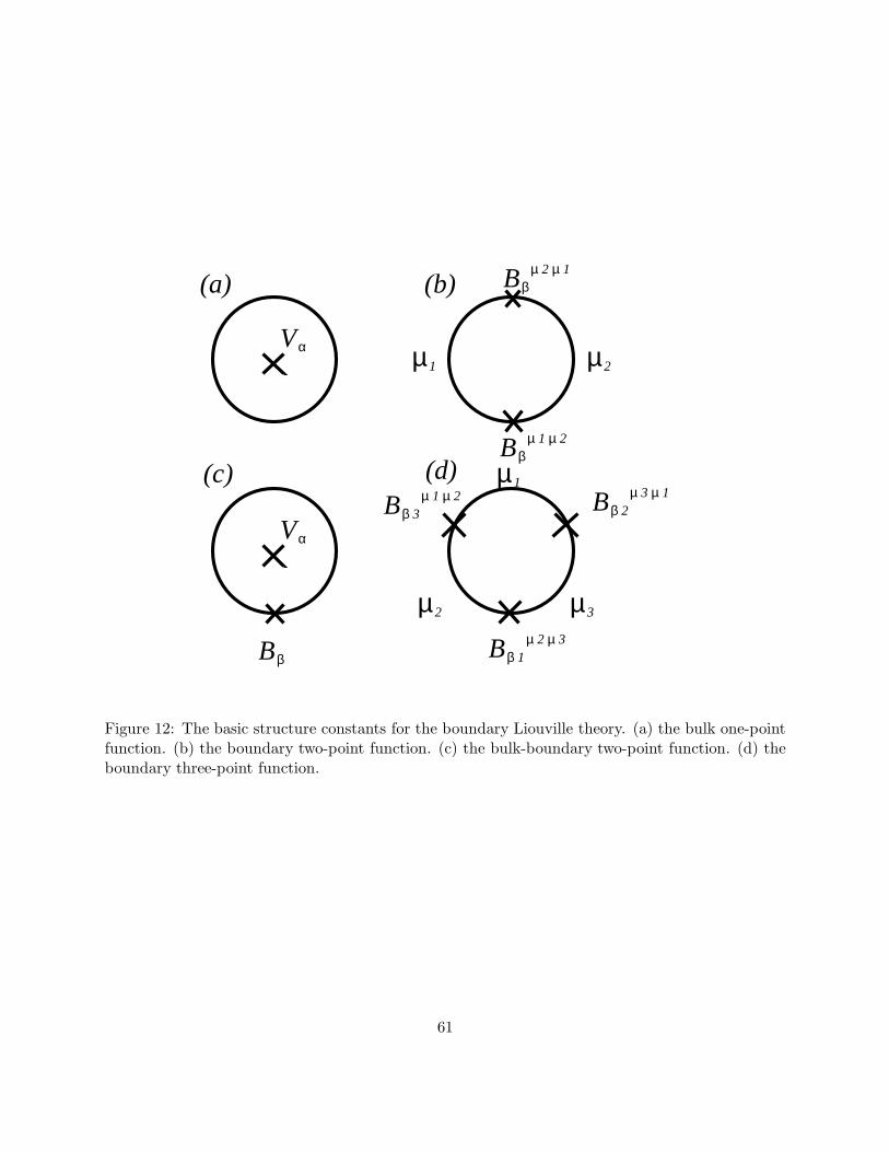
Vα
Vα
Bβ
Bβµ 2 µ 1
Bβµ 1 µ 2
µ1 µ2
µ1
µ2 µ3
Bβ 1µ 2 µ 3
Bβ 3µ 1 µ 2 Bβ 2
µ 3 µ 1
(a)
(c) (d)
(b)
Figure 12: The basic structure constants for the boundary Liouville theory. (a) the bulk one-pointfunction. (b) the boundary two-point function. (c) the bulk-boundary two-point function. (d) theboundary three-point function.
61
To calculate this two-point function, we use the z → x OPE. Since V−b/2 belongs to the degeneraterepresentation, its OPE with any operator begins only with the two primary fields such as
V−b/2Vα = C+[Vα−b/2] + C−[Vα+b/2]. (5.10)
To prove this, note the more general correlator satisfies
0 = 〈:(
1
b2∂2 + T (z)
)V−b/2(z) : Vα(z1) · · · 〉. (5.11)
Taking the z → z1 limit and substituting the general OPE relation
V−b/2(z)Vα(z1) ∼ (z − z1)∆α′−∆α−∆−b/2Vα′ + · · · , (5.12)
we obtain the second order equation for ∆α′ . The solution of the equation yields α′ = α± b/2.Next, we would like to know the fusion coefficient C±. Fortunately (or deliberately), since the
mismatch of the Liouville charge conservation is just the integral multiple of what can be providedby the perturbative treatment of the Liouville potential, we can calculate this by assuming theperturbative calculation saturates the amplitude. Considering the Zamolodchikov innerproductbetween the OPE and the “charge conjugated” out state,
C+ = 〈VQ−α+b/2(∞)V−b/2(1)Vα(0)〉= 〈VQ−α+b/2(∞)V−b/2(1)Vα(0)〉Q,free= δ(0)∞2∆α−b/2 ≡ 1, (5.13)
where in the last line, we have normalized our result properly. Under the same normalization, weobtain
C− = 〈VQ−α−b/2(∞)V−b/2(1)Vα(0)〉= −µ
∫d2z〈VQ−α−b/2(∞)e2bφ(z)V−b/2(1)Vα(0)〉
= −µπγ(2bα− 1 − b2)
γ(−b2)γ(2bα). (5.14)
Collecting these pieces of information, we can determine G−b/2,α as follows
G−b/2,α =|x− x|2∆α−2∆−b/2
|z − x|4∆α[C+U(α− b/2)F+(η) + C−U(α+ b/2)F−(η)], (5.15)
where we have introduced the SL(2,R) invariant cross-ratio:
η =(z − x)(z − x)
(z − x)(z − x). (5.16)
Since the whole two-point function obeys the second order differential equation, we can calculateF±(η). This is essentially the hypergeometric function whose precise form was calculated by BPZ[138], and it is written as
F+(η) = ηαb(1 − η)−b2/2F (2αb− 2b2 − 1,−b2, 2αb − b2, η)
F−(η) = η1+b2−αb(1 − η)−b2/2F (−b2, 1 − 2αb, 2 + b2 − 2αb, η) (5.17)
On the other hand, to calculate the same correlation function, we can also do it by expandingthe bulk operator by the boundary OPE. Since the intermediate states have only two primary fields,
62

the degenerate operator V−b/2 has only two OPE expansion with respect to the boundary operator,namely, B0 and B−b. Particularly, if we concentrate on the coupling to B0, the fusion coefficientwith respect to Vα is of course the one-point function U(α) and the fusion coefficient with respect toV−b/2 is given by R(−b/2, Q) which can be interpreted as the innerproduct between V−b/2 and the“charge conjugated” boundary operator BQ. This bulk-boundary structure constant R(−b/2, Q)can be calculated perturbatively because the charge conservation is violated by just the integralmultiple of b. Assuming the perturbative saturation, we obtain
R(−b/2, Q) = −22∆12µB
∫dx〈V−b/2(i)Bb(x)BQ(∞)〉Q,free
= −2πµBΓ(−1 − 2b2)
Γ(−b2)2 . (5.18)
The coupling to the descendant is also determined as above. Solving the differential equation, weobtain
G−b/2,α =|x− x|2∆α−2∆−b/2
|z − x|4∆α[B+G+(η) +B−G−(η)], (5.19)
where
G+(η) = ηαb(1 − η)−b2/2F (−b2, 2αb − 2b2 − 1,−2b2, 1 − η)
G−(η) = ηαb(1 − η)1+3b2/2F (1 + b2, 2αb, 2 + 2b2, 1 − η), (5.20)
and the information available so far states B− = U(α)R(−b/2, Q).
V− b/2 Vα
V− b/2 + α or Vb/2 + α
V− b/2 Vα
BQ
or BQ+b
B0
or Bb
Figure 13: The auxiliary bulk two-point function can be calculated in two different ways.
Comparing the two different calculation for the same two-point function: (5.15) and (5.19), thefunctional relation for U(α) can be derived. In order to do that, we rewrite F± in terms of G±.Using the inversion formula for the hypergeometric function (A.46), we can rewrite F± as
F+(η) =Γ(2αb− b2)Γ(1 + 2b2)
Γ(1 + b2)Γ(2αb)G+(η) +
Γ(2αb− b2)Γ(−1 − 2b2)
Γ(2αb− 2b2 − 1)Γ(−b2)G−(η)
F−(η) =Γ(2 + b2 − 2αb)Γ(1 + 2b2)
Γ(1 + b2)Γ(2 + 2b2 − 2αb)G+(η) +
Γ(2 + b2 − 2αb)Γ(−1 − 2b2)
Γ(1 − 2αb)Γ(−b2) G−(η). (5.21)
63
Substituting this and comparing the term proportional to G−(η), we obtain the functional relationfor U(α):
− 2πµBΓ(−b2)U(α) =
Γ(−b2 + 2bα)
Γ(−1 − 2b2 + 2bα)U(α− b/2) − πµΓ(−1 − b2 + 2bα)
γ(−b2)Γ(2bα)U(α+ b/2), (5.22)
after substituting C− and working with some algebra.The solution of this functional relation is given by
U(α) =2
b(πµγ(b2))(Q−2α)/2bΓ(2bα − b2)Γ
(2α
b− 1
b2− 1
)cosh(2α−Q)πs, (5.23)
where, instead of µB , we have introduced a new parameter s:
cosh2 πbs =µ2B
µsinπb2. (5.24)
We sometimes use the related quantity σ:
cos2 (2πb(σ −Q/2)) =µ2B
µsinπb2 (5.25)
The calculation for showing that this quantity satisfies the functional relation (5.22) is straightfor-ward. For instance, after dividing the both sides by U(α), use the formula cosh(a−b)+cosh(a+b) =2 cosh a cosh b, and we have cosh πbs. Then, writing this as
√sinπb2, we cancel this term with the
remaining factor Γ(1− b2)Γ(b2) = sin(πb2)/π. The rest of the calculation is simply the applicationof the Γ function formula.
Let us comment on the properties of this solution. The solution is invariant under the dualtransformation b → b−1, µ → µ, s → s, µB → µB (the last transformation for µB is definedsuch that s is invariant under this transformation). With the same reasoning as in the DOZZformula, this solution is unique up to an overall normalization factor. The overall normalizationis determined by the requirement that the residue at 2α = Q − nb reproduces the perturbativecalculation.
5.1.2 Boundary two-point function
Next, we proceed to the determination of the boundary two-point function by Teschner’s trick.Although the basic strategy is the same — we derive the functional equation from the OPE of theboundary degenerate operator, there is a difference concerning the boundary degenerate operator.
For example, it may seem that we have a null vector if we take the boundary operator B−nb/2for a positive integer n because the central charge and the conformal dimension suggest so fromthe Kac formula. However, when we take n = 1, we find from the semiclassical (b→ 0) analysis,
T (x) = −1
4φ2x +
1
2bφxx + π(πµ2
Bb2 − µ)e2bφ, (5.26)
and consequently, the left-hand side does not vanish as follows,
(d2
dx2+ b2T
)e−bφ/2 = πb2(πµ2
Bb2 − µ)e3bφ/2. (5.27)
Since we are dealing with nonnormalizable states, this kind of peculiarity could happen. Therefore,we cannot use the n = 1 degenerate state. However, the n = 2 degenerate state Bss
−b can be used
64
because this satisfies the following third order homogeneous differential equation (we have labeledits cosmological constant by s instead of µB),
(1
2b2∂3 + 2T (z)∂ + (1 + 2b2)∂T (z)
)Bss
−b = 0. (5.28)
The intuitive reason why the third order differential equation is valid is that Bss−b can be regarded
as the limit of the bulk degenerate operator V−b/2 to the boundary. Since the bulk degenerateoperator satisfies the corresponding differential equation we expect the boundary limit obeys thesimilar equation unlike the n = 1 case.43 Using this degenerate operator, we can derive the fusionformula:
Bss−bB
ss′β = c+[Bβ−b] + c0[Bβ] + c−[Bβ+b], (5.29)
which is based on the same reasoning as in the one-point function.Let us consider the auxiliary three-point function 〈Bss
−b(x1)Bss′β (x2)B
s′sβ+b(x3)〉. First, comparing
the result from the x1 → x2 OPE with that from the x1 → x3 OPE, we obtain
d(β + b|s, s′)c−(β) = c+(β + b)d(β|s, s′). (5.30)
We set c+ =1 because this fusion coefficient can be calculated from the zeroth order perturbationtheory. For c−, since the charge non-conservation is 2, we can calculate this, under the perturbativesaturation assumption, as the sum of the the bulk first order perturbation contribution and theboundary second order perturbation contribution. The former contribution is given by
cv− = −µ∫
Imz>0d2z〈e2bφ(z)Bss′
β (0)Bs′s′−b (1)Bs′s
Q−β−b(∞)〉Q,free
= µ
∫
Imz>0d2z
|1 − z|4b2
|z|4bβ |z − z|2b2 , (5.31)
and the latter contribution is given by
cb− =∑
ij
µiµj2
∫
Ci
∫
Cj
dx1dx2〈ebφ(x1)ebφ(x2)Bss′β (0)Bs′s′
−b (1)Bs′sQ−β−b(∞)〉Q,free
=∑
ij
µiµj2
∫
Ci
∫
Cj
dx1dx2|(1 − x1)(1 − x2)|2b2
|x1 − x2|2b2 |x1x2|2bβ. (5.32)
Performing the integration, we obtain
c−(β) = 4µ sin
(πb
2β + i(s+ s′)2
)sin
(πb
2β − i(s+ s′)2
)
× sin
(πb
2β + i(s − s′)2
)sin
(πb
2β − i(s − s′)2
)I0(β) (5.33)
where
I0(β) = −γ(1 + b2)
πΓ(1 − 2bβ)Γ(2bβ − 1)Γ(1 − b2 − 2bβ)Γ(2bβ − b2 − 1). (5.34)
Substituting this into the functional relation, we have to solve
d(β + b|s, s′)d(β|s, s′) = c−1
− (β). (5.35)
43This can be directly seen semiclassically by using the equation of motion.
65
As usual, enforcing the dual relation b → b−1 makes the solution unique up to an overall normal-ization. Using the special function Γb(x) and Sb(x) which have been introduced in appendix A.3,we can write the solution as
d(β|s, s′) =(πµγ(b2)b2−2b2)(Q−2β)/2bΓb(2β −Q)Γ−1
b (Q− 2β)
Sb(β + i(s + s′)/2)Sb(β − i(s+ s′)/2)Sb(β + i(s − s′)/2)Sb(β − i(s − s′)/2)(5.36)
To check this, we use the difference relation of Γb(x) and Sb(x) (four sins are from the shift ofSb. Since each Γb(x) is shifted twice, we obtain four Γ functions, which reproduces I0(β)). Thenormalization of the two-point function is determined by the “unitarity” 44:
d(β|s, s′)d(Q− β|s, s′) = 1. (5.37)
5.1.3 Bulk-boundary correlator
We consider the bulk boundary correlation function. We present the final result [156] first. Weintroduce the Fourier transformation of R(α, β, s), calling it R(α, β, p), as
R(α, β, p) =1
2
∫ ∞
−∞dse4πspR(α, β, s), (5.38)
then the result is given by
R(α, β, p) = 2π(µπγ(b2)b2−2b2)(Q−2α−β)/2bΓb(Q− β)3Γb(2Q− 2α− β)Γb(2α− β)Υ(2α)
Γb(Q)Γb(β)Γb(Q− 2β)
×Sb(p+β + 2α−Q
2)Sb(p+
β − 2α +Q
2)Sb(−p+
β + 2α−Q
2)Sb(−p+
β − 2α +Q
2). (5.39)
Let us sketch the proof. As we discussed before, B−b/2 does not satisfy the fusion rule of
the degenerate operator. However FZZ [2] conjectured that Bs,s±ib−b/2 does satisfy the second order
differential equation. Actually the two-point functions which can be obtained independently fromthis conjecture are consistent with the result of the last subsection. Here, we just assume thisconjecture and set
Bs,s±ib−b/2 Bs±ib,s′
β = [Bs,s′
β−b/2] + c±[Bs,s′
β+b/2], (5.40)
where we have set the fusion coefficient to be 1 as usual in the case where the Liouville charge isconserved. c± is calculated perturbatively and given by
c± = 2
(− µ
πγ(−b2)
)1/2
Γ(1 − 2bβ)Γ(2bβ − b2 − 1)
× sinπb(β ∓ ib(s1 + s2)/2) sin πb2(β ∓ ib(s1 − s2)/2). (5.41)
Now, consider the auxiliary three-point function 〈Vα(z)Bβ(x)ss′B−b/2(y)
s′s〉, where s±s′ = ±ib.Using the conformal invariance, we can map the upper half plane to the disk of a unit radius. Thenthe three-point function can be written as
〈Vα(z)Bβ(x)ss′B−b/2(y)
s′s〉u.h.p= (x− z)−∆β−∆−b/2(x− z)−∆β+∆−b/2(z − z)∆β−2∆α+∆−b/2(y − z)−2∆−b/2
44The meaning of the unitarity is as follows. We regard this relation as 〈β|β〉〈Q − β|Q − β〉. If we realize|Q − β〉 = S|β〉, the above relation means SS† = 1. S can be interpreted as the reflection amplitude of the openstring state. Note that the S matrix is diagonal in this representation.
66
× 〈Vα(0)Bβ(1)ss′Bs′s
−b/2(η)〉disk , (5.42)
where η = (y−z)(x−z)(y−z)(x−z) . We would like to derive the functional relation taking the η → 1 OPE. At
first sight, we cannot solve R from this equation because we cannot evaluate the left-hand sidedirectly. The trick is that when η approaches from the upper and lower, the answer is different sothat we can obtain the closed equations (in other words, there is a monodromy and B is not localwith each other).
The equations are
〈Vα(0)Bβ(1)ss′Bs′s
−b/2(η)〉disk
= R(α, β − b/2; s′)Gα,β(η)eiπbβ/2 + c−(β, s, s′)R(α, β + b/2; s′)Gα,Q−β(η)e
iπb(Q−β)/2
= R(α, β − b/2; s)Gα,β(e−2πiη)e−iπbβ/2 + c−(β, s′, s)R(α, β + b/2; s)Gα,Q−β(e
−2πiη)e−iπb(Q−β)/2,(5.43)
where G is given by the hypergeometric function as
Gα,β(η) = ηbα(1 − η)bβF (b(2α + β −Q− b/2), b(β − b/2), b(2β − b), 1 − η). (5.44)
Solving this equation, we finally obtain R. The answer has been given at the beginning of thissubsection.
5.1.4 Boundary three-point function
We present the boundary three-point function here. The result is [157]
Cσ3σ2σ1
(Q−β3)β2β1
=Γb(2Q− β1 − β2 − β3)Γb(β2 + β3 − β1)Γb(Q+ β2 − β1 − β3)Γb(Q+ β3 − β1 − β2)
Γb(2β3 −Q)Γb(Q− 2β2)Γb(Q− 2β1)Γb(Q)
× (πµγ(b2)b2−2b2)(β3−β2−β1)/2bSb(β3 + σ1 − σ3)Sb(Q+ β3 − σ3 − σ1)
Sb(β2 + σ2 − σ3)Sb(Q+ β2 − σ3 − σ2)
× 1
i
∫ i∞
−i∞dtSb(U1 + t)Sb(U2 + t)Sb(U3 + t)Sb(U4 + t)
Sb(V1 + t)Sb(V2 + t)Sb(V3 + t)Sb(Q+ t), (5.45)
where we have used the notation:
U1 = σ1 + σ2 − β1, V1 = Q+ σ2 − σ3 − β1 + β3
U2 = Q− σ1 + σ2 − β1, V2 = 2Q+ σ2 − σ3 − β1 − β3
U3 = β2 + σ2 − σ3, V3 = 2σ2
U4 = Q− β2 + σ2 − σ3. (5.46)
See (5.25) for the relation among σ, s and µB.We will not delve into the detailed calculation here, but the basic strategy is the same. We use
the conformal bootstrap method to find the functional relation which can be derived by insertingthe degenerate operator B−b.
5.2 ZZ Brane: D0-Brane
Zamolodchikov brothers showed [3] that in the Liouville theory there exists a D0-brane whichis localized in the Liouville direction. We call it the ZZ brane. Semiclassically, this boundarycondition corresponds to the solution of the Liouville equation on the disk which describes the
67
Poincare disk metric (or the Euclidean AdS2 metric on the upper half plane). The solution of theclassical Liouville equation: ∆ϕ = 2R−2eϕ is given by
eϕ(z) =R2
(Imz)2, (5.47)
which means ϕ → ∞ at the boundary.45 Another explanation why the D0-brane is localized inφ → ∞ is that there is a linear dilaton background so that the brane tension which is inverselyproportional to the string coupling constant becomes smaller as the brane goes into the deeper φregion. The purpose of this section is to understand the quantum description of this boundarycondition.
5.2.1 Bulk one-point function
As in the FZZT brane case discussed in the last section, we consider the one-point function whichis given by
〈Vα(z)〉 =U(α|µB)
|z − z|2∆α. (5.48)
The basic strategy is the same as before, so we consider the auxiliary two-point function 〈V−b/2(z)Vα(x)〉.We expand this in two different ways and compare them to obtain the functional relations whichconstrain U(α). First, using the bulk OPE, we obtain
G−b/2,α =|x− x|2∆α−2∆−b/2
|z − x|4∆α[C+U(α− b/2)F+(η) + C−U(α+ b/2)F−(η)] (5.49)
Second, using the boundary OPE, we obtain
G−b/2,α =|x− x|2∆α−2∆−b/2
|z − x|4∆α[B+G+(η) +B−G−(η)] (5.50)
These equations are almost the same as those obtained in the last section. The only differenceis B−(α). If we assume that our results reproduce the Poincare disk metric semiclassically, thephysical distance between the two point will diverge in the limit Imz → 0. Then we expect, fromthe cluster decomposition theorem, that the two-point function factorizes to the product of theone-point functions of each operator. Since the surviving intermediate state on the boundary hereis the identity only, we expect
B−(α) = U(α)U(−b/2) (5.51)
to hold.46 Substituting the inversion formula for the hypergeometric function, we obtain the func-tional relation for U(α) which states
Γ(−b2)U(α)U(−b/2)Γ(−1 − 2b2)Γ(2αb − b2)
=U(α− b/2)
Γ(2α− 2b2 − 1)− πµΓ(1 + b2)U(α+ b/2)
(2αb− b2 − 1)Γ(−b2)Γ(2αb). (5.52)
45Note that the Liouville equation originally describes the constant negative curvature metric. In the semiclassicallimit b → 0, we identify ϕ = 2bφ and R−2 = 4πµb2.
46More precisely, it is U(α)U(−b/2)D(0) from the correspondence with the FZZT brane discussed above. Whilewe take the innerproduct between the boundary operators to be 〈Q|0〉 = 1 in the last section, in this case we haveset D(0) = 〈0|0〉 = 1. This is because we cannot define the natural charge conjugation of the boundary operator inthis boundary condition unlike the FZZT boundary condition.
68
The solutions (after demanding the b → 1/b duality as usual) of this equation are labeled bytwo positive integers m and n and can be written as
Um,n(α) =sin(πb−1Q) sin(πmb−1(2α−Q)) sin(πbQ) sin(πnb(2α−Q))
sin(πmb−1Q) sin(πb−1(2α−Q)) sin(πnbQ) sin(πb(2α −Q))U1,1(α), (5.53)
where the fundamental solution U1,1(α) is given by
U1,1(α) =[πµγ(b2)]−α/bΓ(2 + b2)Γ(1 + 1/b2)
Γ(2 + b2 − 2bα)Γ(1 + b−2 − 2α/b). (5.54)
Since the functional relation here is nonlinear unlike the ones treated so far, it is not obvious (at leastto the author) that there are no other solutions. In any case, we can check these solutions satisfythe functional relation. For example, we transform all the gamma functions into the trigonometricfunctions by the formula Γ(1− x)Γ(x) = π
sinπx ; then we can see the both sides of the equations areequivalent.
Although many solutions labeled by (m,n) exist, only m = 1 survives in the b→ 0 semiclassicallimit. This fact suggests that the m 6= 1 solutions are difficult to interpret as the quantizationof the Poincare disk. Among other solutions, it is believed that the (1, 1) solution has a specialmeaning. Its remarkable property is vanishing of B+
1,1(α), which means that this boundary couplesto the bulk only through the identity operator (and its descendants). This is very interesting. Ifwe regard these boundary conditions as the D0-brane localized in φ→ ∞, it is natural to considerthe (1, 1) state as the ground state of the D0-brane and other states as the discrete excited states.
5.2.2 Boundary states and modular bootstrap
The one-point function obtained above is normalized as Um,n(0) = 1. Though the superficialreason is that the functional relation is nonlinear and determines the normalization uniquely, themore fundamental reason is that we have used the cluster decomposition theorem to derive thefunctional relation. Clearly, for the relation 〈1〉〈1〉 = 〈1〉 to hold, we should have 〈1〉 = 1. In somecases, however, we would like to know the unnormalized one-point function which is not divided by〈1〉unnormalized. In the following, we consider this case.
For this purpose, we use the open/closed correspondence of the cylinder diagram. First, wedefine the open Virasoro character as
χP (τ) =qP
2
η(τ). (5.55)
On the other hand the character for the (m,n) degenerate representation is given by
χm,n(τ) =q−(m/b+nb)2/4 − q−(m/b−nb)2/4
η(q). (5.56)
The modular transformation of this character to the exchange channel is given by
χm,n(τ′) = 2
√2
∫ ∞
−∞χP (τ) sinh(2πmP/b) sinh(2πnbP )dP, (5.57)
where τ ′ = −1/τ . Especially the modular transformation of χ1,1 which corresponds to U1,1 can bewritten as
χ1,1(τ′) = 2
√2
∫ ∞
−∞χP (q) sinh(2πbP ) sinh(2πP/b)dP. (5.58)
69
Then we can see this cylinder amplitude from the closed channel exchange point of view as
χ1,1(τ′) =
∫ ∞
−∞Ψ1,1(P )Ψ1,1(−P )χP (q)dP = 〈1, 1|qH
2 |1, 1〉, (5.59)
where the “wavefunction” for the (1, 1) state is given by
Ψ1,1(P ) =23/42iπP
Γ(1 − 2iP b)Γ(1 − 2iP/b)(πµγ(b2))−iP/b. (5.60)
Comparing this with the normalized one-point function U1,1(α) (5.54), we find that the normaliza-tion is different for the α independent constant. From the derivation above, we should regard (5.60)as the unnormalized disk one-point function which is not normalized by 〈1〉unnormalized. To fix the(P dependent) phase of the wavefunction, we have required the wavefunction to satisfy the bulkreflection property (4.13), which completely determines the unnormalized disk one-point functionup to truly meaningless P independent total phase. This wavefunction can also be seen as theexpansion coefficient of the boundary state by the Ishibashi states
〈1, 1| =
∫ ∞
−∞Ψ1,1(P )〈P |dP, (5.61)
where the Ishibashi states [158] are defined as
〈P |qH2 |P ′〉 = δ(P − P ′)χP . (5.62)
From this (1, 1) wavefunction, we can obtain the (m,n) wavefunction. The P dependence ofthe one-point function derived above suggests
Ψm,n = Ψ1,1(P )sinh(2πmP/b) sinh(2πnbP )
sinh(2πP/b) sinh(2πbP )(5.63)
up to an over all normalization factor. To confirm the normalization to be correct, we compare(5.63) with the open loop diagram which can be obtained by the modular transformation
χm,n(τ′) =
∫ ∞
−∞Ψm,n(P )Ψ1,1(−P )χP (q)dP = 〈m,n|qH
2 |1, 1〉, (5.64)
which shows that the open/closed duality works with this normalization. Note, as a bonus, wehave learned that the open string spectrum which stretches between (1, 1) brane and (m,n) branecontains only the (m,n) degenerate state. This is the interpretation of the (m,n) brane from theCFT point of view.
Similarly we can obtain the wavefunction for the FZZT brane, which is given by
Ψs(P ) =2−1/4Γ(1 + 2ibP )Γ(1 + 2iP/b) cos(2πsP )
−2iπP(πµγ(b2))−iP/b. (5.65)
This expression is of course proportional to the previous FZZT one-point function (5.23). Theexact normalization can be determined as follows, consider the general non-degenerate characterwith P = s/2,
χs/2(q′) =
√2
∫ ∞
−∞χP (q) cos(2πsP )dP. (5.66)
70
This can be interpreted as follows
χs/2(q′) =
∫ ∞
−∞Ψ1,1(P )Ψs(−P )χP (q)dP, (5.67)
which means that the open string stretching from the FZZT brane with the boundary parameters to the (1, 1) ZZ brane is the nondegenerate state with the momentum P = s/2 whose weight is
then ∆ = Q2
4 + s2
4 .Now, using the above boundary states, we can obtain the spectrum stretching between various
branes considered so far. For example, the partition function between (m,n) and (m′, n′) branebecomes
Z(m,n)(m′,n′) =
∫ ∞
−∞Ψm,n(P )Ψm′,n′(−P )χP (q)dP
=
min(m,m′)−1∑
k=0
min(n,n′)−1∑
l=0
χm+m′−2k−1,n+n′−2l−1(q′), (5.68)
which is just the fusion algebra of the degenerate representations. In this way, we can obtainthe operator contents of the (m,n) ZZ brane. They consist of the finite degenerate operators.Furthermore we can obtain the density of states of the FZZT brane by calculating the cylinderdiagram
Zs,s′ =
∫ ∞
−∞Ψs(P )Ψs′(−P )χP (q)dP
=
∫ ∞
−∞ρ(P ′)χP ′(q′)dP ′, (5.69)
where the density of states is
ρ(P ′) = 2√
2
∫ ∞
−∞Ψs(P )Ψs′(−P )e−4πiPP ′
dP
=
∫ ∞
−∞
2 cos(st) cos(s′t)sinh(bt) sinh(t/b)
e−2πiP ′t dt
2π. (5.70)
This expression has a divergence as t → 0 which signals that the FZZT brane is extending alongthe φ direction (on the other hand we can see that the wavefunction for the ZZ brane vanishes asP → 0 which means that the ZZ brane localizes in the φ direction). If we properly regularize thisexpression we should have ρ ∼ 1
2b log(µ) + ρr(p), where ρr(p) is finite. Instead of doing that, weconsider the relative density of states here which is defined as
ρrel(P, s, s′) = ρ(P, s, s′) − ρ(P, sref ), (5.71)
where the reference boundary parameter sref has been introduced. From the discussion in section4.2, we have a nontrivial consistency check about the relationship between the (relative) density ofstates and the boundary two-point function:
ρrel(P, s, s′) = − i
2π
d
dPlog
(d(P |s, s′)d(P |sref )
). (5.72)
Substituting (5.36) into the left-hand side and using the integral formula for the logarithm of thedouble sine function (A.71), we can see that the relation actually holds.
71
However, the change of integration order in (5.69) is not legitimate if s is pure imaginary [155].In this case, we deform the contour of the modular transformation formula as
χα(q′) =√
2
∫
r+iRdβe4πi(α−
Q2
)(β−Q2
)χβ(q), (5.73)
where r is in the range r > max(|σ+|, |σ−|, Q2 ) with σ± = i(s2 ± s1) ∈ R. Now we can change theintegration order, but if we deform the integration in the density of states to the original rangeQ2 + iR, we have other contributions from poles in Sb, which yield the discrete spectrum. Thediscrete spectrum is unitary only if |σ±| < Q, in which case, the discrete spectrum is just the (1, 1)degenerate state. On the other hand, if |σ±| > Q, the nonunitary (m,n) degenerate states appearin the spectrum. There is no discrete spectrum when |σ±| < Q/2.
To conclude this subsection, let us make some comments on the boundary states and spectrumof the open modes.
First, as has been noticed by Martinec [159], the (m,n) boundary states are formally related tothe FZZT boundary states as
|m,n〉 = |FZZT; s(m,n)〉 − |FZZT; s(m,−n)〉, (5.74)
where the boundary parameter s(m,n) is defined as
s(m,n) = i(mb
+ nb). (5.75)
It is interesting to note that the boundary cosmological constants for s(m,±n) have actually thesame value
µB(m,n) = (−1)m√µ
cos(πnb2)√sin(πb2)
. (5.76)
This is possible when s takes the pure imaginary value. In a sense, we can make different FZZTbranes of the same boundary cosmological constant by adding (m,n) ZZ branes, which is one of thefundamental reasons why we have the additional discrete degenerate spectrum in the open stringsstretching between the FZZT branes with an imaginary boundary parameter s. This viewpointand its application to the boundary perturbation theory has been further developed in [160] (seealso [161] and [67] for the discussion on the nature of the monodromy).
Second, for the future application, we consider the spectrum of the open string which stretchesbetween the ZZ branes when c = 1 with a time-like X boson which has the Neumann boundarycondition. The mass formula for the (m,n) degenerate state is given by
Ltotal0 = −(n+m)2
4, (5.77)
which means that the ground state becomes more tachyonic with increasing m or n. While thedynamics of (1, 1) tachyon will be further studied in the later section, the physical meaning of theremaining “heavy” tachyon is rather mysterious.47
Let us further study the spectrum on the (1, 1) brane. In the two dimension, the oscillatorpartition function becomes
Z = qH0η(q)2(1 − q)1
η(q)2= qH0(1 − q) (5.78)
47However see section 6.6 for the nonperturbative contribution from these states.
72

Because of the nature of the degenerate state, the partition function looks non-unitary. 48 The lowenergy on-shell spectrum consists of a tachyon whose mass is (−1), a time-like vector, the ghost andanti-ghost whose energy is zero (recall no ghost decouples). Since the dynamics is one-dimensional,it is not obvious whether this has a deep meaning or not. It is important to note, however, thatthere is no degree of freedom which moves the ZZ brane in the φ direction, which guarantees thatthe ZZ brane is fixed in the φ→ ∞ region.
Finally let us consider the spectrum of the open string stretching between the FZZT brane withboundary parameter s and the (m,n) ZZ brane. The character is given by
∫ ∞
−∞Ψm,n(P )Ψs(−P )χp(q)dP =
m−1∑
k=1−m,2
n−1∑
l=1−n,2χ(s+i(k/b+lb))/2(q
′), (5.79)
where∑n−1
k=1−n,2 denotes the summation over the set k = −n + 1,−n + 3 · · · , n − 1. However,the right-hand side shows that the mass (weight) of the open string becomes imaginary unless s ispure imaginary. Even in that case, the mass is tachyonic. This further shows the difficulty of thephysical interpretation of (m,n) 6= (1, 1) branes. The only meaningful possibility may be the (1, 1)brane. When we take c = 1, the open string state between the FZZT brane and the (1, 1) brane
can be either tachyonic or massive, which is given by m = s2
4 .
5.2.3 Bulk-boundary structure constant
The bulk-boundary two-point function on the ZZ brane is derived by Ponsot [164]. We review hisderivation and result here. The bulk boundary two-point function on (m,n) brane is given by
〈Vα(z)Bβ(x)〉m,n =Rm,n(α, β)
|z − z|2∆α−∆β |z − x|2∆β, (5.80)
where the notation here is β = −ub− vb−1 with positive integers (u, v) which corresponds to the(2v + 1, 2u + 1) degenerate operator. Note that the notation is just for the convenience and Bβhas nothing to do with any exponential operator of the Liouville field. Also, recall that the (m,n)boundary state has only u < n and v < m operators in the spectrum. For simplicity we concentrateon the (1, 2u + 1) operator here (for more general cases, see [164]). The direct derivation of thetwo-point function is as follows.
Consider an auxiliary bulk two-point function 〈V−ub/2Vα〉. This auxiliary two-point functioncan be calculated in two ways: by taking the OPE of the two bulk operators first or by taking theboundary OPE first. Equating the B−ub contribution of the both calculations, we obtain
u∑
k=0
C(α,−ub/2, Q− α+ ub/2 − kb)Um,n(α− ub/2 + kb)Fα−ub/2+kb,−ub/2
[−ub/2 −ub/2α α
]
= Rm,n(α,−ub)Rm,n(−ub/2,−ub)Dm,n(−ub).
(5.81)
Almost all the structure constants in (5.81) have been calculated. Thus Rm,n(α,−ub) is calculablefrom the expression above. First, the three-point function with α1 +α2 +α3 = Q− kb is given by
Ck(α1, α2, α3) =
( −πµγ(−b2)
)k ∏kj=1 γ(−jb2)∏k−1
l=0 γ(2α1b+ lb2)γ(2α2b+ lb2)γ(2α3b+ lb2), (5.82)
48At first glance, there is a contradiction with the generalized no ghost theorem [162, 163]. However, the situationhere just corresponds to the exceptional cases considered there.
73

from the (pre) DOZZ formula (4.7). Second, the one-point function Um,n(α) is given by (5.53).Third, Dm,n(−ub) and Rm,n(−ub/2,−ub) can be set to one as long as the corresponding operatorexists in the boundary spectrum (otherwise zero). 49
Finally, the fusion matrix Fα−ub/2+kb,−ub/2
[−ub/2 −ub/2α α
]is the transformation matrix be-
tween t channel conformal block and s channel conformal block. For the simplest case, we havederived it from the inversion formula of the hypergeometric function. In principle, we can redo thesame procedure to obtain the degenerate fusion matrix. In practice, it is easier to obtain it fromreading off the residue of poles of the known general results. The general fusion matrix has beenfound in [152], which we are not going to derive here. It is given by
Fα−ub/2+kb,−ub/2
[−ub/2 −ub/2α α
]=
u∏
l=1
Γ(bQ+ ub2 + (l − 1)b2)
u−1∏
l=k
Γ(2bα− ub2 + (l + k)b2)
Γ(2bα + lb2)Γ(bQ+ lb2)
×k∏
j=1
Γ(bQ+ (j − 1)b2)Γ(2bQ− 2bα+ ub2 − 2kb2 + (j − 1)b2)
Γ(bQ+ ub2 − jb2)2Γ(2bQ− 2bα+ ub2 − jb2).
(5.83)
Combining these factors, we can calculate Rm,n(α,−ub). The result can be also expressed insomewhat different form as (perhaps up to factor π2)
Rm,n(α,−ub) =
−1
b(πµγ(b2))
12b
(−2α+ub) sin(πb−1Q) sin(πbQ)
sin(πmb−1Q) sin(πnbQ)Γ(bQ)Γ(Q/b)Qb−ub(b−b
−1)
×Γ(2bα− b2)Γ(2b−1α− 1 − b−2)u−1∏
j=0
Γ(2bα − bQ− ub2 + jb2)Γ(bQ+ ub2 + jb2)
Γ(2bα + ub2 − (j + 1)b2)Γ(bQ+ jb2)b1−b(−ub+2j)
× sinπmb−1(2α − ub−Q)
×
u∑
k=0
sinπnb(2α− ub−Q+ 2kb)k−1∏
j=0
sinπb(2α − ub−Q+ jb) sin πb(−ub+ jb)
sinπb(2α+ jb) sin πb(Q+ jb)
. (5.84)
We can check that the expression above becomes zero whenever u > n. Since there is no suchboundary operator in this case, this is obvious physically, but the actual cancellation occurs aftersumming over k and it is nontrivial. This yields a further consistency check on the spectrum of the(m,n) boundary operators.
Finally we note that the above expression is shown to satisfy Hosomichi’s proposal [156].Roughly speaking, if we Fourier transform the two-point function of the FZZT brane with respectto the boundary parameter s as
R(α, β, p) =
∫ ∞
−∞e4πspRs(α, β)ds (5.85)
and perform the further transformation
∫ +i∞
−i∞sin(2πnpb) sin(2πmpb−1)R(α, β, p)dp, (5.86)
49The former is simply the normalization convention of our boundary operators. Note that the nontrivial reflectionamplitude does not exist in this case. The latter is considered to be the ‘no screening charge case’ which means thecase where the spin just adds up with the coefficient 1. The author would like to thank B. Ponsot for clarifying thispoint to the author.
74
then we can obtain the two-point function on the (m,n) ZZ brane up to the factor
−(πµγ(b2))−Q/2bsin(πb−1Q) sin(πbQ)
sin(πmb−1Q) sin(πnbQ)Γ(bQ)Γ(Q/b)Q. (5.87)
Using the explicit formula of the Rs(α, β) (5.39), we can reproduce the direct result in this way.To conclude this section, let us list the remaining structure constants which have not been
derived yet.
• Boundary two-point functions. However, on the same brane, they are trivially set to one(unless zero because of the weight mismatch). On the different branes, they can be nontrivial(though we think it is natural to have one also in this case).
• Boundary three-point functions. Knowing these constants will certainly improve our under-standing of the (m,n) 6= (1, 1) ZZ branes.
5.3 Literature Guide for Section 5
The general boundary conformal theory was pioneered by Cardy [165, 166, 167]. These ideas wereapplied to the boundary Liouville theory in [2], [155]. Besides the various consistency checks donein the original papers, the comparison of those amplitudes reviewed in the main text with the loopgas approach [168, 169, 170] to the two dimensional gravity has been done in [171, 15].
Before the work of ZZ [3], the pseudosphere geometry was studied in [38, 172]. While the ZZbrane is the most natural brane existing in the irrational CFT with a continuum spectrum from theopen string perspective50, the geometrical interpretation of the pseudosphere is surprising. Thoughwe have not treated in the main text, the direct way to see its connection is to calculate correlationfunctions on the pseudosphere by the background field path-integral, which means that we expandthe Liouville field around the classical pseudosphere background as a perturbation in b. In theiroriginal paper [3], they have verified that the calculation reproduces the (1, 1) brane solution up tothe two loop order. The three loop calculation has been done in [173].
6 Applications
In this section, we review (only a few) applications of the bosonic Liouville theory. Some of themare taken from the recent developments and some of them are older ones. Since the realm of thesubject is so vast, we omit the detailed derivation of the many statements in this section. Thereader can find them in the original papers. Even without details, we cannot review all the relatedworks in the main text. We will list other works in the literature guide section. The organizationof this section is as follows.
In section 6.1, we revisit the matrix model as a holographic (gauge/gravity) dual of the openstring theory on the unstable ZZ branes, which provides us a new interpretation and insight of theold matrix models. In section 6.2, we discuss the time-like Liouville theory which is obtained fromthe analytic continuation of the Liouville theory to c = 25. In section 6.3, we discuss a close relationbetween the topological string theory and the Liouville theory. After reviewing the basic propertiesof the topological string theory, we will see that the Liouville theory coupled to the c = 1, R = 1compactified boson can be described by the topological string theory via various dualities.
50The author feels that one cannot imagine any other simple possibility of the open spectrum satisfying the Cardycondition with only the conformal symmetry.
75
In section 6.4, we return to the matrix model description and discuss the decaying D-brane inthe two dimensional string theory from the matrix (and Liouville) point of view. In section 6.5,we discuss the two dimensional black hole which is closely related to the Liouville theory. Thedual matrix model and the brane in this model are also discussed there. In section 6.6, we discussthe nature of the nonperturbative effect encoded in the matrix model partition function from thecontinuum Liouville perspective, where the ZZ type branes play an important role. In section 6.7,we discuss the connection between the branes in the minimal model coupled to the two dimensionalgravity (Liouville theory) and the degenerate Riemann surface.
6.1 Matrix Reloaded
In section 3, we have shown that the closed Liouville theory can be described by the double scalinglimit of the matrix quantum mechanics. There, we have given the interpretation that the c = 1Liouville theory emerges in the continuum limit of the free-boson on the discretized world sheet.However, the new physically deeper interpretation of the matrix quantum mechanics has beenproposed recently by McGreevy and Verlinde [81] (see also [80], [69] for an earlier argument). Wewould like to review the idea quickly.
The idea is that we regard the matrix quantum mechanics as the quantum mechanics of thetachyon field which lives on the N unstable D0-branes (ZZ branes). As is discussed in section 5,the ZZ branes have a tachyon which transforms as an adjoint representation of the Chan-Patongauge group U(N). Its effective action is given by
Seff =
∫dt
1
2Tr(DtT )2 − Tr[V (T )] + · · · , (6.1)
where the kinetic term has been gauged since the ZZ branes also have a non-dynamical gauge field.This action yields clearly the (gauged) matrix quantum mechanics! From the open/closed duality,we expect that the open string dynamics of the D0-branes describes the pure closed string physics(here, the Liouville theory) in an appropriate limit. The appropriate limit is nothing but thedouble scaling limit. Recall that the double scaling limit means the simultaneous limit of gs → 0and N → ∞ with the fixed Fermi level µ.51 In this limit, the physics of D0-branes completelydecouples from the closed string, namely “gravity”. Thus, this observation yields the foundationthat the effective action on the D0-brane is the decoupled tachyon system above (the Maldacenalimit!). In fact, since the Liouville theory is given by the double scaling limit of the tachyon matrixquantum mechanics, we can say that the open/closed correspondence of this system is proved insome sense.
Before considering the physical implication of this new interpretation, we would like to commenton the tachyon potential. While the field theory on the D0-branes is generally unknown, the D0-branes considered here have a free Neumann boson X0 whose spectrum is well-known. The openspectrum is given by the tachyon 1 and the (non-dynamical) gauge field X0. 52 Since the gauge fielddoes not have a kinetic term in the space of dimension one, the actual effect is simply truncating thestates of the matrix quantum mechanics onto the gauge invariant states. As we will see later, thishas an important meaning which gives the strong evidence of the open/closed duality. However,the problem is the tachyon potential. Around T = 0, it is given by the tachyonic (−1 in our unit)mass term from the tree level spectrum, but the higher form of the potential is difficult to obtain.In principle, we can calculate the perturbative S matrix from the boundary correlation functions,
51By the way, as long as we fix µ, the physics does not change if we change N or gs. This is called the “newduality” in [81].
52The subtlety concerning the ghost has been discussed in the previous section.
76

but the evaluation of the effective potential is rather difficult. It is natural to assume the boundaryCFT type effective potential which has been reviewed in section 2 (Actually, we expect T = eX
0
becomes the time-like CFT). In any case, in the double scaling limit, the detailed shape of thepotential fortunately does not matter.
Let us list evidence and comments about this duality, some of which we will discuss furtherlater in this section.
• The gauging of the tachyon by coupling to the world line gauge field plays a significant rolewhen we consider the partition function of the compactified X0 theory. As we have seen insection 3, the matrix quantum mechanics does not describe the continuum Liouville theoryunless we restrict the spectrum to the gauge invariant sector. Otherwise the T-duality becomesruined for example. We will discuss the physical interpretation of including the twisted sectorlater in this section in relation to the two dimensional black hole. As for the Liouville theory,the gauging of the matrix quantum mechanics naturally solves this problem.
• From the discretized surface point of view, it is ambiguous whether we should take the parityeven potential or the more general potential which does not preserve the parity. Empirically,the matrix-Liouville correspondence chooses the general potential (or we should divide thefinal answer by two in the parity even case). However, the proposal here naturally yields theleft-right asymmetric potential, so this is indeed consistent with the Liouville theory choice.
• As we will see in part II of this review, there is stronger evidence of this kind of duality.The same reasoning also applies to the supersymmetric extension of the Liouville theory.Particularly the matrix model dual for the N = 1 super Liouville theory coupled to c = 1matter has been proposed in Takayanagi-Toumbas [174] and Douglas et.al. [16]. The ideais that we regard the matrix quantum mechanics of the tachyon on the unstable D0-braneswhich exist in the (type-0A or type-0B) super Liouville theory as the dual description ofthe parent super Liouville theory. In fact, it can be shown that the one-loop super Liouvillepartition function and the proper scattering amplitudes are exactly reproduced from thematrix quantum mechanics which is different for 0A and 0B.
• While closed tachyon fluctuations become the collective excitations of the Fermi surface, theextra addition of an eigenvalue corresponds to the addition of an unstable D0-brane into thetheory in this new interpretation. Actually, the matrix model description of the decay andthe Liouville theory direct calculation match [175], [176], [114] as we will see later in thissection. In particular, the emission rate of the closed string and the final state distributionbeyond the lowest order are given by the semiclassical matrix quantum mechanics.
• Let us rephrase this in the string field theory language [177], [178]. The D0-brane quantummechanics is in a sense an open string field theory because we treat the theory fully quantummechanically (not only on mass shell). The new interpretation of the duality states that theopen string field theory does know the closed string theory as the collective field theory ofthe D0-brane Fermi surface. In this sense, Sen’s conjecture is marvelously realized in theLiouville theory though the open string field theory is the “holographic dual” of the closedstring theory. It is important to note that the rolling tachyon can be regarded as the rollingeigenvalue of the fermion. In the later time, this can be interpreted as the disturbance of theFermi surface, i.e. the closed string background. The tachyon matter [179] is just the closedtachyon coherent states and conserves the energy. We will see this issue more closely in thefollowing sections.
77
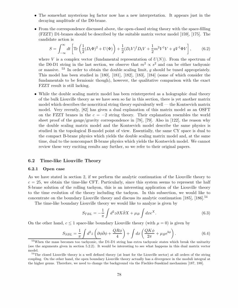
• The somewhat mysterious leg factor now has a new interpretation. It appears just in thedecaying amplitude of the D0-brane.
• From the correspondence discussed above, the open-closed string theory with the space-filling(FZZT) D1-branes should be described by the suitable matrix vector model [159], [175]. Thecandidate action is
S =
∫ ∞
−∞dt
[Tr
(1
2(DtΦ)2 + U(Φ)
)+
1
2(DtV )†DtV +
1
2m2V †V + gV †ΦV
], (6.2)
where V is a complex vector (fundamental representation of U(N)). From the spectrum ofthe D0-D1 string in the last section, we observe that m2 ∝ s2 and can be either tachyonicor massive. 53 In order to obtain the double scaling limit, g should be tuned appropriately.This model has been studied in [180], [181], [182], [183], [184] (some of which consider thefundamentals to be fermionic though), however, the qualitative comparison with the exactFZZT result is still lacking.
• While the double scaling matrix model has been reinterpreted as a holographic dual theoryof the bulk Liouville theory as we have seen so far in this section, there is yet another matrixmodel which describes the noncritical string theory equivalently well — the Kontsevich matrixmodel. Very recently, [82] has given a dual explanation of this matrix model as an OSFTon the FZZT branes in the c = −2 string theory. Their explanation resembles the worldsheet proof of the gauge/gravity correspondence in [78], [79]. Also in [122], the reason whythe double scaling matrix model and the Kontsevich model describe the same physics isstudied in the topological B-model point of view. Essentially, the same CY space is dual tothe compact B-brane physics which yields the double scaling matrix model and, at the sametime, dual to the noncompact B-brane physics which yields the Kontsevich model. We cannotreview these very exciting results any further, so we refer to their original papers.
6.2 Time-like Liouville Theory
6.2.1 Open case
As we have stated in section 2, if we perform the analytic continuation of the Liouville theory toc = 25, we obtain the time-like CFT. Particularly, since this system seems to represent the halfS-brane solution of the rolling tachyon, this is an interesting application of the Liouville theoryto the time evolution of the theory including the tachyon. In this subsection, we would like toconcentrate on the boundary Liouville theory and discuss its analytic continuation [185], [186].54
The time-like boundary Liouville theory we would like to analyze is given by
STBL = − 1
π
∫d2z∂X∂X + µB
∫dxeX . (6.3)
On the other hand, c ≤ 1 space-like boundary Liouville theory (with µ = 0) is given by
SSBL =1
π
∫d2z
(∂φ∂φ+
QRφ
4
)+
∫dx
(QKφ
2π+ µBe
bφ
). (6.4)
53When the mass becomes too tachyonic, the D1-D1 string has extra tachyonic states which break the unitarity(see the arguments given in section 5.2.2). It would be interesting to see what happens in this dual matrix vectormodel.
54The closed Liouville theory is a well defined theory (at least for the Liouville sector) at all orders of the stringcoupling. On the other hand, the open boundary Liouville theory actually has a divergence in the moduli integral atthe higher genus. Therefore, we need to change the background via the Fischler-Susskind mechanism [187, 188].
78

closed tachyon
unstable D-brane
µ = 1/geff
Figure 14: The schematic picture of the decaying D-brane and the closed tachyon excitation fromthe open string field (= fermion) perspective.
Thus the formal analytic continuation b → i and Wick rotation X = iφ lead to (6.3). The reasonwhy we call it “formal” is that it is not trivial at all whether we can analytically continue the c ≤ 1Liouville theory to b → i. Actually this “analytic continuation” has an ambiguity which seems tocorrespond to the different choice of the vacuum states in the time-dependent quantum theory.
We here consider the bulk one-point function and the boundary two-point function each of whichhas a specific physical significance. The former can be interpreted as the interaction between theclosed string states and the boundary (brane) states. In the space-like Liouville theory (c ≤ 1), thelatter can be interpreted as the reflection amplitudes. This goes as follows. In the minisuperspaceapproximation, the zero-mode wavefunction is given by
Ψp(φ) → e+ipφ +Rb(p)e−ipφ, φ→ −∞, (6.5)
where φ is regarded as space and Rb is what is called the reflection amplitude which can be readoff from the boundary two-point function as
Rb(p) = db(Q/2 − ip). (6.6)
Intuitively, we can imagine the process where an incoming wave eipφ reflected from the Liouvillepotential becomes an outgoing wave with the phase shift (or S matrix) Rb(p). Note that we haverequired that the wave should damp as φ→ ∞ in order to obtain this wavefunction uniquely. Nowwe try to “analytically continue” this to b→ i. Wick rotating the coordinate as φ→ −iX and theenergy as p→ −iω, we obtain
Ψω(φ) → e−iωX + di(ω)eiωX , X → −∞, (6.7)
where di(ω) is given bydi(ω) = 〈e−iωXe−iωX〉TBL, (6.8)
79
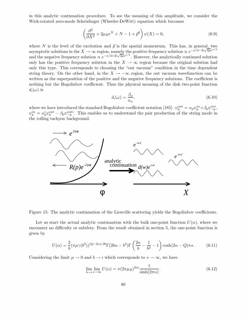
in this analytic continuation procedure. To see the meaning of this amplitude, we consider theWick-rotated zero-mode Schrodinger (Wheeler-DeWitt) equation which becomes
(∂2
∂X2+ 2µBe
X +N − 1 + ~p2
)ψ(X) = 0, (6.9)
where N is the level of the excitation and ~p is the spatial momentum. This has, in general, twoasymptotic solutions in theX → ∞ region, namely the positive frequency solution ∝ e−x/4−2i
√2µex/2
and the negative frequency solution ∝ e−x/4+2i√
2µex/2. However, the analytically continued solution
only has the positive frequency solution in the X → ∞ region because the original solution hadonly this type. This corresponds to choosing the “out vacuum” condition in the time dependentstring theory. On the other hand, in the X → −∞ region, the out vacuum wavefunction can bewritten as the superposition of the positive and the negative frequency solutions. The coefficient isnothing but the Bogoliubov coefficient. Thus the physical meaning of the disk two-point functiondi(ω) is
di(ω) =βωαω, (6.10)
where we have introduced the standard Bogoliubov coefficient notation [185]: ψoutp = αpψinp +βpψ
in∗−p ,
ψinp = α∗pψ
outp − βpψ
out∗−p . This enables us to understand the pair production of the string mode in
the rolling tachyon background.
analyticcontinuation
e2ipφ
R(p)e -2ipφ
φ X
e -iwX
d(w)e iwX
e -iwX
Figure 15: The analytic continuation of the Liouville scattering yields the Bogoliubov coefficients.
Let us start the actual analytic continuation with the bulk one-point function U(α), where weencounter no difficulty or subtlety. From the result obtained in section 5, the one-point function isgiven by
U(α) =2
b(πµγ(b2))(Q−2α)/2bΓ(2bα − b2)Γ
(2α
b− 1
b2− 1
)cosh(2α−Q)πs. (6.11)
Considering the limit µ → 0 and b→ i which corresponds to s→ ∞, we have
limb→i
lims→∞
U(α) = π(2πµB)2iα1
sinh(2πα). (6.12)
80

Let us check the correctness of this procedure by comparing this result with what can be obtainedfrom the boundary perturbation of the time-like boundary Liouville theory which we have reviewedin appendix B.4. Of course the perturbation theory can be used only to evaluate 〈e−nX〉 for apositive integer n. This can be calculated as
〈e−nX(z)〉TBL = µnB〈e−nX(z)
∫dx1 · · · dxn
∏
i
eX(xi)〉free
= |z − z|−n2/2µnB(2π)nΓ(n+ 1)Γ(−n), (6.13)
where we have used∫dxe−nx−e
x= Γ(−n) as the zero-mode integration. Analytically continuing
this result for general momentum, we expect to obtain
〈e−iωX(z)〉TBL = |z − z|−2∆ω(2πµB)iωπ
i sinhπω, (6.14)
which is the same amplitude we have obtained as the analytic continuation of the boundary Liouvilletheory.
Then we consider the analytic continuation of the boundary two-point function, which is a littlebit subtler. From the b ≤ 1 result in section 5, we have
d(β|s, s′) =(πµγ(b2)b2−2b2)(Q−2β)/2bΓb(2β −Q)Γ−1
b (Q− 2β)
Sb(β + i(s + s′)/2)Sb(β − i(s + s′)/2)Sb(β + i(s− s′)/2)Sb(β − i(s − s′)/2). (6.15)
Taking the s = s′ → ∞ limit, we obtain55
lims→∞
d(ω) =
(π2µb1−b
2
Γ(1 − b2)
)(Q−2ω)/bΓb(−Q+ 2ω)
Γb(−2ω +Q)
1
Sb(ω)2. (6.16)
The problem is that Γb(x) is not defined in the b→ i limit. In fact, Γb(x) has a simple pole atx = −mb − n/b for positive integers n and m. In the b → i limit, it is easy to see that infinitelymany poles accumulate to the integer multiple of i. Therefore (6.16) appears to be meaningless atfirst sight.
Nevertheless, we can formally transform (6.16) so that we obtain an integral expression which wecan interpret physically by choosing the proper contour. The existence of the contour dependenceis because we are dealing with the time-dependent theory. From the formula found in appendix(A.3), we have
Γb(2ω −Q)
Γb(Q− 2ω)
1
Sb(ω)2
= Yb(ω)b2ω/b−2bω−1/b2+b2 Γ(2ω/b− 1/b2)Γ(2ωb− 1 − b2)Γ(−2ω/b+ 1)Γ(−2ωb)
Γ2(−ω/b+ 1)Γ2(−bω), (6.17)
where
Yb(ω) ≡ Γb(2ω)Γb(−ω)2
Γb(−2ω)Γb(ω)2=
∏
m,n≥0
(2ω + Ω
−2ω + Ω
)(−ω + Ω
ω + Ω
)2
. (6.18)
We have used the infinite product formula (A.62) for the Γb function found in appendix A.3 withΩ = mb+ n/b.
55For simplicity, we consider one kind of brane or a diagonal element of the several kinds of branes. However, theinclusion of the off-diagonal elements does not affect most of the following argument. Note that s− s′ is finite in theµ→ 0 limit.
81
To give a precise meaning to the Yb(ω) in the b → i limit, we first take b = iβ with real β andthen we take β → 1 limit. In this limiting prescription, Yb(ω) keeps to be a pure phase [185]. Theactual analytic continuation keeping this property can be found in the original paper. Omittingthe detailed calculation, we present the final result
Yi(ω) = −eiθ(ω), (6.19)
where the phase is given by
θ(ω) =1
2
∫ ∞
0
dτ
τ
sin(4ωτ) − 2 sin(2ωτ)
sinh2(τ). (6.20)
Therefore, the whole two-point function is now analytically continued to
di(ω) =(2πµ)2iωeiθ
4 cosh2(πω). (6.21)
The remarkable property of this expression is that this reproduces the result of the minisuperspaceapproximation in the large ω limit [185] (though it is not clear at least to the author why theminisuperspace approximation becomes better in the large ω limit). Note that we would have hada different result which does not reproduce the minisuperspace approximation if we had taken thelimit of Y (ω) from the other side.
Thus the analytic continuation of the space-like boundary Liouville theory to c = 25 time-like boundary Liouville theory has a subtlety concerning the analytic continuation of the specialfunctions. In addition, there is no physically satisfying principle how to remove the ambiguity ofthe analytic continuation procedure for three- or higher multi-point functions.
6.2.2 Closed case
Let us now consider the analytic continuation of the bulk Liouville correlation functions to c = 25[189], [190]. The time-like Liouville action which we would like to study is given by
STL =1
4π
∫d2z
(−4∂X∂X + 4πµe2X
). (6.22)
We would like to understand the theory from the analytic continuation b → i of the space-likeLiouville theory
S =1
4π
∫d2z
√g(gab∂aφ∂bφ+QRφ+ 4πµe2bφ
)(6.23)
as in the boundary Liouville theory considered in the last subsection. Here, we specifically focus onthe two-point function and the three-point function. As we will see, the two-point function can beanalytically continued without much trouble, but the three-point function has many subtle points.
Let us first study the two-point function. For c ≤ 1, the two-point function is given by
D(α) = (πµγ(b2))(Q−2α)/b γ(2bα − b2)
b2γ(2 − 2α/b + 1/b2). (6.24)
Setting b = iβ, we take the β → 1 − 0 limit. Then, we have
d(ω) = limβ→1−0
−(πµγ(−β2))iω/βΓ(1 − iω/β)Γ(1 + iωβ)
Γ(1 + iω/β)Γ(1 − iωβ). (6.25)
82
Since the first term diverges in this limit, we introduce the renormalized cosmological constant asµR ≡ |µγ(−β2)|. Fixing the value of µR, we can now take the µ→ 0, β → 1 − 0 limit:
d(ω) → −(πµR)iωe−πω, (6.26)
which reproduces the minisuperspace amplitude [189].56
Let us go on to the three-point function. The c ≤ 1 result is given by the DOZZ formula
C(α1, α2, α3) =[πµγ(b2)b2−2b2
](Q−∑3i=1 αi)/b
× Υ′(0)Υ(2α1)Υ(2α2)Υ(2α3)
Υ(α1 + α2 + α3 −Q)Υ(α1 + α2 − α3)Υ(α1 − α2 + α3)Υ(−α1 + α2 + α3). (6.27)
Along the same line of reasoning and calculation, Strominger and Takayanagi [189] proposed thefollowing expression for the b = i three-point functions
〈e2iω1Xe2iω2Xe2iω3X〉 = C(ω1, ω2, ω3) (6.28)
where the obvious conformal factors are suppressed and the structure constant is given by
CST (ω1, ω2, ω3) = (πµR)i∑
j ωje2πω×
× exp
∫ ∞
0
dτ
τ
1
sinh2 τ/2
sin2 ωτ +∑
j
(sin2 ωjτ − sin2 ωjτ)
, (6.29)
where ωjs are defined as
ω =1
2(ω1 + ω2 + ω3), ω1 =
1
2(−ω1 + ω2 + ω3)
ω2 =1
2(ω1 − ω2 + ω3), ω3 =
1
2(ω1 + ω2 − ω3). (6.30)
The first factor comes from the prefactor of the DOZZ formula and the exponential factor comesfrom the careful evaluation of the b→ i limit of the Upsilon functions. The puzzle of this formulaappears when we take the naive limit ω1 → 0. We expect this reproduce the two-point functionderived above. However this does not hold. The fact that the correlation functions with ω2 6= ω3
survives in this limit is especially puzzling, for this breaks the conformal invariance.In [190], Schomerus has made an attempt to solve this puzzle. His strategy is basically as follows.
When we take the b → i limit, the obvious obstacle is the nonexistence of the Γb. However, thefunctional recursion relation itself does not suffer from this subtlety. Then we solve the recursionrelation for the pure imaginary b, which is unique if we demand the dual relation at the same time.This corresponds to solving the “Liouville theory” whose central charge is less than 1. Now wecan take the limit b → i as we take the limit b → 1 in the usual DOZZ formula. The limit exists,but it is different according to whether we consider the Euclidean continuation or the Minkowskicontinuation.
56While the renormalization of the Liouville potential is also needed for b = 1, the physical interpretation in b = iseems not so clear to the author. Particularly, in the open case, the boundary cosmological constant never needs tobe taken infinitesimally. Note that the value of the boundary cosmological constant does have a physical meaning forthe full S-brane (µB = 1 corresponds to the no tachyon vacuum). This may or may not result from the fundamentaldifference between the open string tachyon and the closed string tachyon.
83

In the Euclidean limit, we have the Runkel-Watts theory [191] as a limit of the unitary minimalmodels. In the Minkowski limit, the essential difference from the Strominger-Takayanagi proposalis the additional factor
P (ω1, ω2, ω3) =
(1 + Θ(ω)
3∏
i=1
Θ(ωj)
), (6.31)
where we have introduced the step function
Θ(x) =
−1 for x < 0+1 for x > 0.
This factor does not make difference if all the ωj are positive. Remarkably the factor solves thepuzzling issue stated above as it gives zero unless ω2 = ω3 in the ω1 → 0 limit. Can we obtainthe correct reflection amplitude in this limit? This seems difficult, for the identity operator is notthe simple α→ 0 limit of Φα = eiωX as in the Runkel-Watts theory. However, we can read off thereflection amplitude from the behavior under ω1 → −ω1, which yields d(ω) = (πµR)2iωe−2πω asdesired.
6.3 Topological String Theory
6.3.1 Topological sigma model, topological Landau-Ginzburg model
The easiest construction of the topological theory is twisting the supersymmetric theory. Since theaction of the supersymmetric theory is invariant under the fermionic transformation, the changeof its spin makes it a scalar BRST invariant theory. In addition, the energy momentum tensorcan be represented as the anticommutator of the SUSY generator, which follows from the SUSYalgebra. Therefore, the energy momentum tensor is automatically BRST exact, which guaranteesthe topological nature. In the following, we twist two dimensional (1, 1) supersymmetric theoriesto make topological world sheet theories. If we couple these twisted theories to the (topological)gravity in some sense, they become topological string theories.
First of all, we consider twisting the supersymmetric sigma model (see e.g. [192, 193]). In thiscase, there are two different ways to twist the theory. What we call the A-model is given by thefollowing action
S = 2t
∫d2z
(1
2gIJ∂zφ
I∂zφJ + iψizDzχ
igii + iψizDzχigii −Riijjψ
izψ
izχ
jχj), (6.32)
where ψiz is (1, 0) form and χi is scalar as fields on the world sheet. We take CY3 as the targetspace. The supersymmetric (BRST) transformation is given by
δφi = iαχi
δφi = iαχi
δχi = δχi = 0δψiz = −α∂zφi − iαχjΓijmψ
mz
δψiz = −α∂zφi − iαχjΓijmψmz . (6.33)
The action is BRST invariant up to the surface term from the general argument of the supersym-metric theory. This can be rewritten in a manifestly BRST invariant way as
S = it
∫
σd2zQ,V + t
∫Φ∗(K), (6.34)
84

where V = gij(ψiz∂zφ
j + ∂zφiψjz). The total derivative term is the pull back of the Kahler form of
the target space which is given by
∫Φ∗(K) =
∫d2z(gij∂zφ
i∂zφj − gij∂zφ
i∂zφj). (6.35)
This depends only on the Kahler class of the original target space and the degrees of map from theworld sheet. Therefore, the contribution is simply from the world sheet instanton. The remarkablefeature of this model is that the physical amplitudes do not depend on the complex structure ofthe targetspace at all (Indeed the variation comes only from the BRST exact term Q,V ). Onthe other hand, the dependence on the Kahler moduli is determined from the world sheet instantoncontribution.
Similarly, if we twist the left and right fermions on the world sheet differently, the twisted theorybecomes what we call the B-model. The action is given by
S = 2t
∫d2z
(1
2gIJ∂zφ
I∂zφJ + iηi(Dzρ
iz +Dzρ
iz)gii + iθi(Dzρ
iz −Dzρ
iz) +Riijjρ
izρjzηiθkg
kj
).
(6.36)Its BRST transformation is given by
δφi = 0δφi = iαηi
δηi = δθi = 0δρi = −αdφi. (6.37)
The action can be rewritten in a manifestly BRST invariant form. Defining V = gij(ρiz∂zφ
j +
ρiz∂zφj), we obtain
S = it
∫d2zQ,V + tW, (6.38)
where W is given by
W =
∫d2z
(−θiDρi −
i
2Riijjρ
i ∧ ρjηiθkgkj). (6.39)
We can see that the B-model does not depend on the Kahler moduli but only depends on thecomplex moduli of the target space.
The other model we would like to discuss is the Landau-Ginzburg model [194]. Using superfieldsXi, we have the following action
S =
∫d2zd4θXiX i +
∫d2zd2θW (X) + c.c.
=
∫d2z(|∂xi|2 + |∂iW |2) + (ρi∂ψi + ρi∂ψi + ρi∂i∂jWρj + ψi∂i∂jWψj), (6.40)
where we have considered the B-model so that ψ is a world sheet scalar and ρ is a world sheetone-form. The BRST transformation is given by
δxi = ψi + ψi
δψi = −∂iWgii
δψi = ∂iWgii
δρi = −∂xi
85
δρi = −∂xi.δxi = 0 (6.41)
This model is not a CFT even at the classical level, but the energy momentum tensor is BRST exact.Therefore, the correlation function does not depend on the two dimensional metric. Then, rescalingthe metric as g → λ2g, we can see the path integral localizes at the points where dW = 0. As aresult, any correlation function can be evaluated at the extrema of W . The nontrivial contributionwe should evaluate in the path integral is simply the one-loop determinant. However, this cancelsout almost completely except the zero-mode because of the supersymmetry. From the evaluationof the Gaussian integral
∫d2xi exp(−|λ∂iW |2), the contribution from the bosonic zero-mode x0
i isgiven by
Zb = λ−2n(HH)−1, (6.42)
where H is the Hessian of W . On the genus g world sheet, the number of the fermionic zero-modesare g for each ρ and one for each ψ from the index theorem, so their contribution is given by
Zf = λ2nHgH. (6.43)
Combining them, we finally have the total contribution from the zero-mode: Z = Hg−1. Applyingthis calculation, we can easily obtain the correlation functions on the world sheet with any genus.Assuming one superfield for simplicity, we can write them explicitly
〈F1 · · ·FN 〉g =
∮F1 · · ·FN (W ′′)g
W ′ , (6.44)
where the integration contour is a large circle which encircles all the poles. Intuitively speaking,W ′′ can be regarded as the operator which inserts a handle into the world sheet.
6.3.2 Landau-Ginzburg model for c = 1 Liouville theory
Let us consider the c = 1 Liouville theory compactified on the circle whose radius is R = 1. Thefirst claim here [195, 196] is that this theory is equivalent to the Landau-Ginzburg topologicalstring theory with the superpotential W = −µX−1. This superpotential is singular, but we canalso regard this theory as a twisted Kazama-Suzuki SU(2)/U(1) coset theory with level k formallyanalytically continued to k = −3. The primary fields of this Landau-Ginzburg theory can bewritten as Xk−1. On the other hand, the (physical) primary field of the Liouville theory coupled tothe c = 1, R = 1 compactified boson can be classified by the integer momentum k because the Xspace is compactified and the momentum becomes quantized. Then the proposed correspondenceis Tk = Xk−1 up to leg factors.57 The claim is that the correlation functions (scattering amplitude)calculated from the Landau-Ginzburg theory are the same as those obtained by the matrix model.
By using the basic facts about the Landau-Ginzburg theory that we have introduced in thelast subsection, let us see the simplest example. Consider the tachyon three-point function on thesphere 〈Tk1Tk2Tk3〉0. The previous result (6.44) yields
〈Tk1Tk2Tk3〉0 = Res
(xk1−1xk2−1xk3−1
x−2
)= δk1+k2+k3,0. (6.45)
Though this example seems almost trivial, it is generally known that these calculations reproducethe matrix model results [195, 196]. In addition, the loop calculations can be basically done by
57However, the leg factor always diverges when R = 1, so it is natural to define the renormalized operator whoseleg factor is omitted as Tk = Xk−1. We have done the same renormalization in the DMP formula. See (3.147).
86

using the handle operator which we have introduced in the last subsection. However, to perform theintegration over the moduli space properly, we should introduce the contact terms. Furthermore,we should change the picture of the vertex operator with the negative momenta k in order to pickout the correct gravitational descendant which is necessary to integrate over the moduli space.58
Considering all these, we can show that all correlation functions including the partition functionare the same as those from the matrix model calculation at any loop. However, the derivation ofthe contact term from the first principle is still lacking, so we will not delve into the detail anyfurther.
Assuming this correspondence, we would like to show [199] that the c = 1 Liouville theory canbe understood as the topological B-model on a certain CY3 via the correspondence between theLandau-Ginzburg theory and the topological string on CY [193]. As we will see later, the dualitychain enables us to calculate the partition function of the topological string on this CY3 exactly,which matches the all-order matrix model calculation. This means that we have proved the LiouvilleLandau-Ginzburg correspondence indirectly. Since the critical dimension of the topological stringis 3, we consider the following superpotential
G(X) = −X−10 +X2
1 +X22 +X2
3 +X24 . (6.46)
The addition of massive fields does not change the behavior in the IR from the Landau-Ginzburgpoint of view. Therefore nothing has changed as long as we consider the behavior of X0. If weattribute the U(1) charge as q0 = −2, qi = 1, (i 6= 0), then the superpotential G(X) has a charge 2.Since we would like to gauge this U(1) charge, we further introduce a new field P whose charge is−2 in order to cancel U(1) anomaly. This gauged supersymmetric theory has the following potentialwhich can be obtained from the direct dimensional reduction of the d = 4 superQED:
U =1
2e2D2 + |G|2 + |p|2|∂iG|2 + (A2
2 +A23)
(4|p|2 + 4|x0|2 +
4∑
i=1
|xi|2), (6.47)
with the D term condition
D = −e2(−2(|p|2 + |x0|2) +
4∑
i=1
|xi|2 − r
). (6.48)
where r is the F.I. parameter and A2, A3 are from the second and third component of the 4d vector.Let us first consider the r ≫ 0 case. In this case we have the vacuum condition p = 0,
A2 = A3 = 0 and∑4
i=1 |xi|2 − 2|x0|2 = r, so G(X) = 0. Since the fluctuation becomes massiveunless this condition is satisfied, the IR theory is on G(X) = 0. Further division by the U(1) gaugesymmetry of X suggests that they are naturally regarded as the inhomogeneous coordinates onWCP4
−2,1,1,1,1. That is to say, this theory is just the sigma model on the toric CY3. In addition,
from the condition∑4
i=1 |xi|2 − 2|x0|2 = r and the fact that the metric of the sigma model is givenby the pull back of the original flat metric (though the renormalization makes it flow into the Ricciflat one), we can see that the size of the CY manifold is given by r. The actual form of the CY3
can be seen as follows. Fixing X0 = 159, we obtain
1 = X21 +X2
2 +X23 +X2
4 . (6.49)58On the very intuitive level, this can be explained as follows. Just as we practically carry out the supermoduli
integration by the picture change in the superstring calculation, we replace the integration over the moduli spacewith the calculation of correlation functions in Witten’s topological gravity [197, 198] by the picture change.
59Since X0 is the singular point of the potential, it is infinitely far away in the field space. Therefore, there is noobstruction to suppose X0 6= 0.
87
This is the deformed conifold whose original singularity is A1.On the other hand, by studying the behavior when r ≪ 0, we can show this theory is equivalent
to the Landau-Ginzburg theory with the superpotential G(X). To see this, we first note that thevacuum is given by xa = A2 = A3 = 0 with a = 1 · · · 4 and x0 → ∞ with finite |p| in this limit.Considering the fluctuation around the vacuum solution, we obtain the effective superpotential
W (X) = 〈p〉G(X) (6.50)
if we ignore the massive excitations.The important point here is the fact that the B-model does not depend on the Kahler moduli
at all. However, the F.I. parameter r is the size of the manifold in the sigma model perspective, sothis is just the Kahler moduli. We can also see explicitly that the F.I. term is indeed a BRST exactterm in the gauged non-linear sigma model action. Therefore, although this gauged theory looksdifferent in the different r limit, these are equivalent as the B-model. This proves the equivalenceof the B-model on the deformed conifold and the topological Landau-Ginzburg theory with thesuperpotential X−1
0 . Combining this fact with the Liouville Landau-Ginzburg correspondence, wecan see the following Ghoshal-Vafa conjecture [199] “The c = 1, R = 1 Liouville theory is equivalentto the topological B-model on the deformed conifold.” to be plausible.
6.3.3 Gopakumar-Vafa duality
Let us pause here for a moment and review the Gopakumar-Vafa duality [200, 201, 202] briefly. Tobegin with, let us see the partition function of the A-model topological string more closely. Thepartition function with g > 1 is defined as
F (t) =
∫
Mg
d3g−3Υd3g−3Υ〈3g−3∏
k=1
∫µkG
−∫µkG
−〉, (6.51)
where µ is the Beltrami differential and G− is the supersymmetric current. From the BRST (SUSY)algebra, we regard the supersymmetric current as the antighost b of the bosonic string. The indextheorem states that the complex dimension of the target space should be three in order to absorball the fermionic zero-modes only by these insertions. This shows that the critical dimension of thetopological string is three.
Using the duality between M-theory [201, 202], Gopakumar-Vafa60 calculated the partitionfunction of the topological A-model whose target space is the resolved conifold. For g > 0, we have
Fg = g2g−2s
[(−1)g−1χg
2ζ(2g − 2)
(2π)2g−2− χg
(2g − 3)!
∞∑
n=1
n2g−3e−2πns
], (6.52)
where χg is the (virtual) Euler characteristic of the moduli space of the genus g Riemann surface
whose precise value is given by χg =B2g
2g(2g−2) . s is the area of the S2 which is the deformation
parameter (Kahler moduli) from the conifold. Similarly, the lower genus calculation shows
F0 =1
g2s
[−ζ(3) +
π2
6s+
i
4πs2 − 1
12s3 +
∞∑
n=1
e−2πns
n3
](6.53)
and
F1 =1
24s+
1
12log(1 − e−2πs). (6.54)
60Recently Ooguri-Vafa [78] gave the purely world sheet derivation of this calculation.
88
The Gopakumar-Vafa duality claims that this closed A-model partition function (and otherphysical quantities) transforms into the open A-model on the deformed conifold. This is also calledthe “large N duality” because of the natural connection with the AdS/CFT (or gauge/gravity) cor-respondence. From the AdS/CFT point of view, the rough idea is as follows. We consider wrappingtopological A-branes (which becomes D6-branes in the superstring embedding) on the S3 in thedeformed conifold. Taking into account the fact that the gauge theory living on the branes shouldbe topological, it is given by the U(N) Chern-Simons theory on the S3. In addition, Witten [203]conjectured that this topological open A-model decouples from the closed sector completely. Thisfact is equivalent to the automatic Maldacena limit from the AdS/CFT perspective. Furthermore,since the size of S3 does not affect the topological A-model at all, we can take the conifold limitfreely. Now, from the AdS/CFT analog, the gravity dual should correspond to the closed topolog-ical string theory in the deformed background without branes. The claim of Gopakumar-Vafa isthat it is the closed A-model on the resolved conifold. The parameter correspondence is given by
s = iλ
gs = iλ
N, (6.55)
where λ is the ’t Hooft coupling of the gauge theory.To check the duality, we compare the partition function of the Chern-Simons theory. Since the
Chern-Simons theory has been solved, this comparison is possible. The partition function of theChern-Simons theory is given by
e−Z =1
(N + k)N/2
N−1∏
j=1
[2 sin
(jπ
N + k
)]N−j, (6.56)
where the renormalized ’t Hooft parameter is given by λ = 2πNk+N . We can see the actual equivalence
of the partition function by expanding this expression and performing the resummaion.The particular point to which we would like to pay attention is the nonperturbative contribution
of the Chern-Simons theory to its partition function. This is the part where we cannot write thecontribution as the ’t Hooft (or Feynman) diagram, and it corresponds to the lowest order in s foreach genus. For g > 1, the nonperturbative part is given by
Fg,n.p. =B2g
2g(2g − 2)s2g−2. (6.57)
For g = 0, 1, it is given by
F0,n.p. =s2
2log(s) (6.58)
and
F1,n.p. = − 1
12log(s), (6.59)
respectively. Actually this is from the measure factor of the path integral in the Chern-Simonstheory. When we expand the path integral around A = 0, the residual global gauge freedom is U(N).Therefore, the measure factor contribution to the partition function is essentially log(Vol(U(N))).The volume of the group was calculated by a mathematician [204], which is given by
Vol(U(N)) =(2π)N
2/2+N/2
G2(N + 1), (6.60)
89
where G2(x) is a kind of double gamma function whose defining property is G2(x+1) = Γ(x)G2(x),G2(1) = 1. In our notation, this is essentially the inverse of Γb(x) with b = 1 (times (2π)x/2).61
The logarithm of this expression can be expanded asymptotically as
logG2(N + 1) =N2
2logN − 1
12logN − 3
4N2 +
1
2N log 2π+ ζ ′(−1) +
∞∑
n=2
B2g
2g(2g − 2)N2g−2, (6.61)
which clearly explains the nonperturbative part of the partition function of the Chern-Simonstheory.
6.3.4 Relation to the Liouville theory
Contemplating on the previous result, we notice that the partition function of the c = 1 Liouvilletheory on the R = 1 circle (3.100) has a striking resemblance to the logarithm of the volume of theU(N) group which represents the non-perturbative contribution to the gauge theory. We wouldlike to consider the duality which connects these.
The duality between R = 1 Liouville theory and the topological string theory has already beendiscussed. It is given by the B-model on the deformed conifold. Now, we apply the large N conifoldtransition here. Then the closed B-model on the deformed conifold should be equivalent to the openB-model on the resolved conifold (holomorphic Chern-Simons theory on CP1). In fact, this is justthe mirror symmetry of the A-model large N transition. However, note that this duality is strongerin the A side because the mirror of the deformed conifold on B is the s→ 0 limit of the A-model onthe resolved conifold.62 Hence, by the mirror symmetry, the s → 0 limit, i.e. the nonperturbativepart of the A-model, reproduces the partition function of the closed topological B-model on thedeformed conifold which yields the Liouville partition function.
Though the above statement may sound very complicated, the gist is that the Liouville partitionfunction is given by the log of the U(N) group volume from the chain of dualities. By the way,according to the Dijkgraaf-Vafa proposal, we can argue, without resorting to the mirror symmetry,that the partition function of the closed string on the deformed conifold is given by the Gaussianmatrix model (which is not the c = 1 matrix quantum mechanics). Since the usual matrix modelis defined with the division by the U(N) volume, its log naturally gives the Liouville partitionfunction. In addition, the Dijkgraaf-Vafa correspondence yields the more general matrix duals ofthe conifold deformations. It is interesting to see whether these deformations can be understoodfrom the c = 1 Liouville language. See e.g [91, 122] for a recent discussion on the subject.
6.4 Decaying D-brane
Generally, D-branes in the bosonic string theory are unstable. The on-shell description of theunstable D-brane has been reviewed in section 2. We would like to apply this technique to thebranes existing in the Liouville theory. Though the method can be applied to both the ZZ braneand the FZZT brane, we consider the decay of the (ZZ) D0-brane here anticipating the relationbetween D0-brane decay and the rolling fermion from the top of the potential [175], [114], [207].63
61Note that b = 1 means c = 1 in the Liouville theory, which seems to indicate the relation to the c = 1 Liouvilletheory.
62The exact mirror of finite s is also known [205], [206]. In this case, the B-model theory becomes the matrix modelwith the unconventional measure factor, which becomes sin(λij) after the diagonalization.
63However, note that the classical probe eigenvalue has been discussed in [81] to be described by the decayingFZZT brane with a special boundary parameter. See also [176], [208] for a related discussion.
90
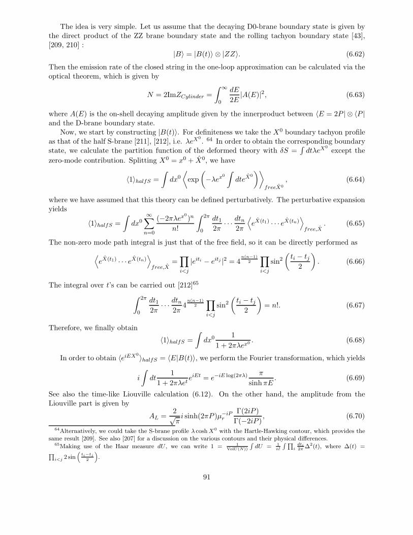
The idea is very simple. Let us assume that the decaying D0-brane boundary state is given bythe direct product of the ZZ brane boundary state and the rolling tachyon boundary state [43],[209, 210] :
|B〉 = |B(t)〉 ⊗ |ZZ〉. (6.62)
Then the emission rate of the closed string in the one-loop approximation can be calculated via theoptical theorem, which is given by
N = 2ImZCylinder =
∫ ∞
0
dE
2E|A(E)|2, (6.63)
where A(E) is the on-shell decaying amplitude given by the innerproduct between 〈E = 2P | ⊗ 〈P |and the D-brane boundary state.
Now, we start by constructing |B(t)〉. For definiteness we take the X0 boundary tachyon profileas that of the half S-brane [211], [212], i.e. λeX
0. 64 In order to obtain the corresponding boundary
state, we calculate the partition function of the deformed theory with δS =∫dtλeX
0except the
zero-mode contribution. Splitting X0 = x0 + X0, we have
〈1〉halfS =
∫dx0
⟨exp
(−λex0
∫dteX
0
)⟩
freeX0
, (6.64)
where we have assumed that this theory can be defined perturbatively. The perturbative expansionyields
〈1〉halfS =
∫dx0
∞∑
n=0
(−2πλex0)n
n!
∫ 2π
0
dt12π
· · · dtn2π
⟨eX(t1) · · · eX(tn)
⟩
free,X. (6.65)
The non-zero mode path integral is just that of the free field, so it can be directly performed as
⟨eX(t1) · · · eX(tn)
⟩
free,X=∏
i<j
|eiti − eitj |2 = 4n(n−1)
2
∏
i<j
sin2
(ti − tj
2
). (6.66)
The integral over t’s can be carried out [212]65
∫ 2π
0
dt12π
· · · dtn2π
4n(n−1)
2
∏
i<j
sin2
(ti − tj
2
)= n!. (6.67)
Therefore, we finally obtain
〈1〉halfS =
∫dx0 1
1 + 2πλex0 . (6.68)
In order to obtain 〈eiEX0〉halfS = 〈E|B(t)〉, we perform the Fourier transformation, which yields
i
∫dt
1
1 + 2πλeteiEt = e−iE log(2πλ) π
sinhπE. (6.69)
See also the time-like Liouville calculation (6.12). On the other hand, the amplitude from theLiouville part is given by
AL =2√πi sinh(2πP )µ−iPr
Γ(2iP )
Γ(−2iP ), (6.70)
64Alternatively, we could take the S-brane profile λ coshX0 with the Hartle-Hawking contour, which provides thesame result [209]. See also [207] for a discussion on the various contours and their physical differences.
65Making use of the Haar measure dU , we can write 1 = 1VolU(N))
∫dU = 1
n!
∫ ∏i
dti2π
∆2(t), where ∆(t) =∏
i<j 2 sin(
ti−tj
2
).
91

from the calculation in section 5, where we have defined the renormalized cosmological constant asµr = πµ0γ(b
2), b2 → 1. Combining these, we obtain
A = At(E = 2P )AL(P ) = 2√πie−iE log(2πλ)eiδ(P ). (6.71)
Note that we have reproduced the proper leg factor eiδ(P ). Since it is a pure phase, the emissionrate is not affected. Now, we can calculate the emission rate and energy,
N =
∫ ∞
0
dE
2E|const|2, (6.72)
which diverges logarithmically in the infrared and ultraviolet. In addition, the emitted energydiverges linearly (because the emitted energy is given by E =
∫dE|const|2). Note that the final
state produced by the decay is a coherent state of the form
|ψ〉 ∼ e∫∞0
dp√2Ea†pAp |0〉. (6.73)
If Sen’s conjecture is correct, the decaying D-brane energy changes into some different form. Theabove lowest emission rate calculation indicates that it becomes closed string tachyons. However,the result has an apparent divergence. We will see in the following the nature of this divergencefrom the matrix quantum mechanical point of view. Anticipating the result, we will see that thequantum treatment of the D-brane cures the divergence. The divergence here is just from localizingthe eigenvalue at a point, whose energy should be divergent in the quantum mechanics.
Let us move on to the matrix model calculation. The useful picture to keep in mind is figure16. The tachyon scattering is described by the collective excitation of the Fermi surface and theD0-brane is described by the excitation of the eigenvalue. In the later time, the decaying D0-brane approaches the Fermi surface and can be regarded as the fluctuation of the Fermi surface.This is the intuitive picture of the rolling D0-brane into the closed tachyon background from thematrix quantum mechanical point of view. Note that we have used here the wave packet picturedeliberately to ensure the semiclassical picture.66
Suppose we would like to add a new rolling eigenvalue (D0-brane) to the matrix quantummechanical system. From section 3, this is described by the relativistic (right) chiral fermion fieldoperator (similar consideration can be done for the left part)
ΨR(τ, t) =1√2π
: exp
[i√π
∫ τ
ΠS − S′dτ ′]
: . (6.74)
Single fermion states are obtained by acting with the operator on the filled Fermi sea. However, ifwe consider the wave packets which have very small overlap with the Fermi sea, we can effectivelytreat them as acting on the Fock vacuum. The state ΨR(τ, t)|0〉 can be expanded by the bosoniza-tion formula (3.117) as the superposition of the incoming tachyon states or the outgoing tachyonstates. We are interested in the outgoing expansion. Using the mode expansion (3.129) and thesemiclassical S matrix elements (3.130), we obtain
√2πΨR(t− τ + log
µ
2)|0〉 = exp
[2i√π
∞∑
n=1
1
n!
∫ ∞
0
dk√8π2k2
∫ 0
−∞dk1 · · · dkneiθ(k)
(i√2πµ
)n−1 Γ(1 − ik)
Γ(2 − n− ik): (a†k1 − ak1) · · · (a†kn
− akn) : δ(±|k1| · · · ± |kn| − k)
]|0〉, (6.75)
66The semiclassical description of the fermionic eigenvalue from the bosonic collective field has a small subtlety.See [213] for a recent discussion on this point.
92
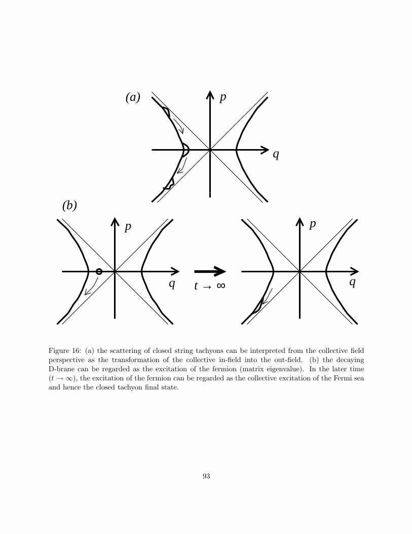
t → ∞
p
p p
q
q q
(a)
(b)
Figure 16: (a) the scattering of closed string tachyons can be interpreted from the collective fieldperspective as the transformation of the collective in-field into the out-field. (b) the decayingD-brane can be regarded as the excitation of the fermion (matrix eigenvalue). In the later time(t→ ∞), the excitation of the fermion can be regarded as the collective excitation of the Fermi seaand hence the closed tachyon final state.
93

where eiθ(k) = −2ike−i log λ and t− τ = − log λ2 . The lowest term is given by
exp
[2i√π
∫ 0
−∞
dk1√8π2k2
1
eiθ(|k|)a†k1
]|0〉. (6.76)
Recalling that the collective field S and the tachyon T differs by the leg pole factor, this is thesame final state calculated from the continuum Liouville field approach (6.73).
What about the rest of the terms in the expansion? If we only keep terms with all creationoperators, the amplitude corresponds to the disk diagrams with any number of tachyon vertexoperators. That is to say, it describes the multi-particle decaying process. Note this is a predic-tion from the matrix model, and whether this amplitude can be obtained from the Liouville diskamplitude is an interesting open question. Furthermore, terms with both creation and annihilationoperators have more µ−1 than the inserted vertices. These terms are naturally regarded as thecontribution of the world sheet with many boundaries. Since the closed S matrix has been treatedsemiclassically, the contribution of the world sheet with handles has not been considered above.For a more detailed argument, see the original paper [114].
Though the matrix model calculates the higher order effects, the situation does not seem im-proved at first sight because the emitted energy remains infinite. As we stated above, however, thisis a wrong setup quantum mechanically. This issue has been studied in [175], [114], [214]. Actually,the appropriate wavefunction should be multiplied to the chiral fermion creation operator. Forexample, if we consider the definite energy state, we obtain
∫dτeiE(t−τ)ΨR(t− τ)|0〉 =
∫dτeiE(t−τ)e
i2√π∫ dp
2π√
2pe−ip(t−τ)a†pAp |0〉, (6.77)
which simply projects the final state onto a definite energy state. Therefore, the energy conservationis manifest. The lesson from here is that it is necessary to treat D-brane quantum mechanically inorder to obtain the proper rolling tachyon energy which should be finite.
Let us finally consider the effect of (unstable but) static D0-brane on the scattering amplitudes.In the matrix model language, this corresponds to the localized eigenvalue at λ = 0. By thecollective field method, the effective change in the Hamiltonian is shown to be
H =1
2p2 − 1
2λ2 +
1
λ2+ µ. (6.78)
See [114] for the derivation of this Hamiltonian. Intuitively speaking, the extra eigenvalue (fermion)produces the repulsive effect which is the Calogero-Moser type. The equation of motion under thepotential is
d2
dt2λ− λ− 2
λ3= 0 (6.79)
which can be solved exactly
λ = a
√cosh2(t− σ) + b, b = −1
2
(1 −
√1 − 8
a4
), (6.80)
where a and σ are integration constants. From this explicit solution, we can calculate the time delayof the scattering. Concentrating on the large (negative) λ region where we can write τ = − log(−λ),the time delay between the given x and back can be calculated from the above explicit solution as
t′ − t = 2τ + log
(a4
4
)(6.81)
94
Using the relation ǫ± = ±(p± λ)λ in the large λ region, we have
ǫ−(t+ τ) =a2
2
√1 − 8
a4. (6.82)
In order to obtain the S matrix elements67, we use the relation ǫ−(t + τ) = ǫ+(t′ − τ) whichfollows from the definition of t′ (i.e. at the time t′, the particle is located at λ but with the minusmomentum as opposed to the incoming particle). Then, substituting (6.81) and (6.82), we obtainthe non-linear relation between incoming and outgoing waves:
ǫ−(t+ τ) = ǫ+
(t+ τ + log(
1
2
√ǫ−(t+ τ)2 + 2)
)(6.83)
We can obtain the S matrix by expanding ǫ as has been done in section 3. The surprising conse-quence is that the S matrix is modified only at the order g2, which means that the disk amplitudeswith any on-shell closed vertex operators are actually zero. It is an interesting open questionwhether this property can be derived from the continuum Liouville field approach. The vanishingof the one-point function can be explained as follows. Since the Neumann X direction forces theenergy and momentum of the on-shell vertex operator to be zero, the vanishing property of theone-point function on the ZZ brane in the p→ 0 limit makes the whole amplitude vanish. For theT-dualized version of this conjecture, see section 6.6 (particularly around the equation (6.152)).
6.5 2D Black Hole
In this section, we review the physics of the 2D black hole and its relation to the Liouville theory.
6.5.1 SL(2,R)/U(1) coset model
Witten [215] has discovered that the SL(2,R)/U(1) WZW model admits the semiclassical proper-ties of the 2D black hole and he proposed that a string theory propagating in this exactly solvableCFT describes the string theory in the 2D black hole. Here, we briefly review this string theoryand its connection with the Liouville theory (or, strictly speaking, a certain kind of 2D noncriticalstring theory).
To begin with, we introduce the gauged WZW model. The action for the ungauged SL(2,R)WZW model at level k is given by
SWZW =k
8π
∫d2z
√hhabtr(g−1∂agg
−1∂bg) +ik
12π
∫
Bd3yǫabctr(g−1∂agg
−1∂bgg−1∂cg), (6.84)
where g is an element of the SL(2,R) and B is a three dimensional manifold whose boundary isgiven by the world sheet Riemann surface. We would like to gauge the following U(1) subgroup ofthe global symmetry of this theory g → agb−1:
a = b−1 = h = 1 + iǫσ2. (6.85)
To do this, we introduce a connection field Ai which transforms under the gauge transformation asδAi = −∂iǫ. Then we replace the ordinary derivative with the covariant derivative so that the space
67Alternatively we can just use the MPR formalism here. We will use this formalism to obtain the loop scatteringamplitudes of the same model in the different context in section 10.1.
95

dependent transformation ǫ(z) becomes a symmetry of the theory. As a consequence we obtain thegauged action
Sgauged = SWZW +k
π
∫d2z(Atr(iσ2g
−1∂g) +Atr(iσ2∂gg−1) +AA(−2 + tr(−σ2gσ2g
−1))). (6.86)
We fix the gauge by imposing the Lorentz (Landau) gauge condition, so we demand ∂aAa = 0.This can be solved in the two dimension as
A = ∂XA = −∂X. (6.87)
Substituting this into the action and picking up the ghost action from the Jacobian of the changeof variables from A to X, we obtain the following gauge fixed action
Sgf = SWZW +k
π
∫d2z∂X∂X +
1
π
∫d2z(B∂C + B∂C), (6.88)
where the ghost system is a spin (1, 0) fermion system. In addition, since the gauged U(1) iscompact, X is compactified on the circle of radius
√k (after rescaling the kinetic term as a con-
ventionally normalized boson). To obtain this action, we have used the global transformation of g[216].
So far, the treatment has been exact in the quantum mechanical sense. However, to see theconnection between this action and the 2D black hole, it is better to do the different gauge fixing.Since the following gauge fixing is semiclassical, we should understand the procedure is exact onlyin the limit k → ∞. The gauge fixing is done by requiring the following form of the group action
g = cosh r + sinh r
(cos θ sin θsin θ − cos θ
). (6.89)
After substituting this into the above action (6.86) and performing the Gaussian integral, we obtainthe gauge fixed action
S =k
π
∫d2z(∂r∂r + tanh2 r∂θ∂θ), (6.90)
where the determinant of the Gaussian integral has been neglected. Therefore we can see that thesemiclassical SL(2,R)/U(1) WZW model is equivalent to the nonlinear sigma model whose metricis given by
ds2 = k(dr2 + tanh2 rdθ2). (6.91)
However, the consistent condition for the string background requires the one-loop Ricci flatness ofthe target space, and this metric does not satisfy this condition. To overcome this difficulty, weshould recall the neglected determinant of the Gaussian integral over A, which probably providesthe dilaton background. We determine the induced dilaton background by requiring that the one-loop Einstein equation Rµν = −2∇µ∇νΦ should hold. Then the dilaton background is given byΦ = 2 log cosh r. Of course, the procedure stated above is valid only semiclassically and highercorrections are needed when k is small which may drive us from the 2D black hole description.
By the way, to obtain the Minkowski version of the above metric, we rotate θ as θ = it andtake the periodicity for t to be infinite. Thus the Minkowski metric becomes ds2 = dr2− tanh2 rdt2
which indeed has a (Minkowski) black hole property after extending the coordinate system. Fromthe gauged WZW model point of view, this corresponds to the gauging of the noncompact U(1)subgroup. Dijkgraaf-Verlinde-Verlinde [216] has studied this semiclassical equivalence quantum
96

mechanically by using the minisuperspace approximation. Though it is interesting, here we willnot delve into the detail any further.
Returning to the SL(2,R)/U(1) WZW model, we try to obtain the correlation functions of thetheory. Since the direct use of the action is inconvenient, we introduce the free field (Wakimoto)representation of the algebra [217]. We first introduce a (1,0) βγ superghost system and a Coulombgas free boson as follows
S =
∫d2z
(1
π∂φ∂φ+
QR
4πφ+
1
π(β∂γ + β∂γ)
), (6.92)
where the background charge is given by Q2 = 1k−2 . Using this action, we define the following
current
J+ = iβ
J3 = βγ +1
Q∂φ
J− = −iβγ2 − i2
Qγ∂φ+ ik∂γ. (6.93)
Via the free field OPE (for our convention, see appendix A.1), we can check the following currentalgebra
J+(z)J−(0) =k
z2− 2J3(0)
z+ · · ·
J3(z)J±(0) = ±J±(0)
z+ · · ·
J3(z)J3(0) = −k2
z2+ · · · (6.94)
which indeed yield the level k SL(2,R) algebra.68 The energy momentum tensor of this theory canbe calculated by the Sugawara construction (or we can directly calculate it because they are free),
T = −β∂γ − (∂φ)2 +Q∂2φ. (6.95)
The central charge is given by c = 3kk−2 .
Now we would like to define the vertex operator in order to calculate the correlation function.Since SL(2,R) does not have a finite dimensional unitary representation, there might be somedifficulties. Requiring that the Casimir J3 and J2 = −1
2(J+J−+J−J+)+J3J3 have a real eigenvalue,we find that the corresponding vertex operator is given by
Tjm(z) = γj−me−2Qjφ, (6.96)
where j takes the same value as in the Liouville momentum, namely j is real or j = −12 + ip where
p is real. Furthermore m takes a real value but the available values are determined by a given j.For example, for j = −1
2 + ip with real p, we can take any real m, but for real j, we have twodifferent representations. One is the highest or lowest representation with j +m or j −m integerrespectively, and the other is the supplementary series with neither j +m nor j −m integer. Theconformal dimension of this operator is given by
∆jm = −j(1 + j)
k − 2. (6.97)
68Our convention is t1 = σ1/2, t2 = σ2/2, t
3 = iσ3/2 and J± = J1 ± iJ2.
97
However, this is not the end of the story. While the current algebra and the vertex operatorsrepresented by the free field indeed provide the correct OPE of the current algebra, most of thecorrelation functions turn out to be zero if we calculate the actual correlation function. This isbecause of the “momentum” and ghost number conservation from the zero-mode path integral ofthe boson and the ghost. To remedy this difficulty, we take the screening charge trick. We add thefollowing term to the action
δS = Q =
∫d2zJ(z) =
∫d2zββe2Qφ, (6.98)
whose weight is one and this does not spoil the differential equation which the current algebrashould satisfy (Knizhnik-Zamolodchikov equation). This can be shown by the following OPE
J3(z)J(w) ∼ regJ+(z)J(w) ∼ reg
J−(z)J(w) ∼ ∂
∂w
(e2Qφ
z − w
). (6.99)
Inserting this term into the correlation function, (at least as long as the charge nonconservation isgiven by the integer unit) we can render them non-zero.
Now we are ready to write down the action of the free field (Wakimoto) representation for theSL(2,R)/U(1) model. After gauge fixing by the Landau gauge, it is given by
S =
∫d2z
(1
4π(∂aφ)2 +
QR
4πφ+
1
π(β∂γ + β∂γ) +Mββe2Qφ+
+1
4π(∂aX)2 +
1
π(B∂C + B∂C) +
1
π(b∂c+ b∂c)
), (6.100)
where X is compactified on the circle of radius√k. For this whole action to be conformally
invariant, the total central charge should vanish, which yields the condition k = 94 and Q = 2.
The BRST symmetry of this theory comes from the diffeomorphism of the world sheet and thegauged U(1), whose BRST charge are given by
QDiff =
∮c(z)
(Tmatter +
1
2Tbc
)
QU(1) =
∮C(z)
(J3 + i
√k∂X
). (6.101)
The BRST invariance under U(1) determines the physical vertex operator as
Vjm = γj−me−2Qjφe2im√
kX. (6.102)
Moreover, the usual diffeomorphism BRST invariance and the compactness of X requires
2j + 1 = ±2
3m
m =1
2(n1 + n2k)
m = −1
2(n1 − n2k), (6.103)
where n1 and n2 are integers.
98
At this point, we would like to see the (semiclassical) relation between this free field represen-tation and the sigma model whose target space is the 2D black hole. To do so we bosonize theβγ ghost. 69 This can be written as β = i∂veiv−u, γ = eu−iv. Then the vertex operator for thescreening charge becomes V = i∂veiv−u+2Qφ (for the left moving part). Now, using the fact that
[QU(1), B] = i∂v +1
Q∂φ+ i
√k∂X (6.104)
holds, we can rewrite the vertex operator for the screening charge as
V ≃ e−u+ive−u+iv
(1
Q∂φ+ i
√k∂X
)(1
Q∂φ+ i
√k∂X
)e2Qφ (6.105)
up to BRST exact terms. However, since the bosonized ghost u and v always appear as thecombination −u+iv, the both contribution cancel in every contraction of these operators. Thereforewe can ignore the factor in practice. Then the action becomes
S =
∫d2z
[1
4π(∂aφ)2 +
QRφ
4π+
1
4π(∂aX)2 +M
(1
Q∂φ+ i
√k∂X
)(1
Q∂φ+ i
√k∂X
)e2Qφ
].
(6.106)This action can be seen from the noncritical string point of view (recall Q = 2.) as the 2D stringperturbed not by the cosmological constant (tachyon) but by the discrete state operator.
On the other hand, we can regard this as a sigma model whose metric is given by
Gφφ = 1 +Mπ
Q2e2Qφ
GφX = iMπ√k
Qe2Qφ
GXX = 1 −Mπke2Qφ. (6.107)
In addition if we introduce θ = X + if(φ), f ′(φ) = 1e2φ−1
and φ = log cosh r we reproduce thesemiclassical black hole metric (6.91) which has been introduced by Witten. We have two commentshere. First, the last transformation needs a quantum correction. Second, the transformation to thesigma model is given by the “complex” transformation which seems a little bit strange. However,if we stick to the Minkowski signature, this is not a problem as we can see from the way i entersthe game [218].
Let us move on to another interpretation of the 2D black hole or SL(2,R)/U(1) model. FZZ[219] and Kazakov-Kostov-Kutasov (KKK) [220] conjectured that the model is also equivalent tothe sine-Liouville theory. We first introduce the sine-Liouville theory and show several pieces ofevidence of this equivalence. 70 The action of the sine-Liouville model is given by
S =1
4π
∫d2z
[(∂aφ)2 + (∂aX)2 +QRφ+ 4πλebφ cos
√k(XL −XR)
], (6.108)
where Q2 = 1k−2 and b = 1
Q as in the above case. Similarly X is compactified on the circle of the
radius√k. As in the Liouville theory Q = 2 is the critical dimension. The corresponding vertex
operator is given byVj;mm ⇐⇒ eipLXL+ipRXR−2Qjφ, (6.109)
69See appendix A.1 for our conventions70The direct proof can be given for the supersymmetric extension of this duality, which we will review in the later
section 12. It is also interesting to note that the claim (6.106) and (6.108) describe the same physics is the bosonicanalog of the conjectured duality in the N = 2 super Liouville theory. See section 11.2 and 12.3.
99

where, with the given integers n1, n2, m and m, the momenta are
pL =n1√k
+ n2
√k
pR =n1√k− n2
√k. (6.110)
We would like to see the equivalence of the two-point functions 〈Vj1m1Vj2m2〉 on the sphere. Ifwe take m = m, the conservation law enforces m1 = −m2 and j1 = j2. We first calculate this two-point function in the free field representation. The ghost conservation, with consideration of theanomaly on the sphere, or the conservation of the zero-mode of φ which gives the same condition,leads to
〈Vj,m(1)Vj,−m(0)〉 =⟨γj−mγj−me−2Qjφe2im/
√kX(1)γj+mγj+me−2Qjφe−2im/
√kX(0)
×M sββe2Qφ(∞)
[∫d2zββe2Qφ
]s−1⟩, (6.111)
where s = 2j + 1 and we have fixed three points by using the SL(2,C) invariance of the worldsheet. Since the contribution of the bc ghost is trivial, we have not apparently included. Although,this expression is only meaningful when s is an integer, the pole at the integer s is believed to begiven by this expression as in the Liouville theory.71 Because this expression is given in terms ofthe free field, the calculation is straightforward. The result is given by
〈Vj,m(1)Vj,−m(0)〉 = (−πMγ(Q2))sγ(1 + j −m)γ(1 + j +m)sγ(1 − s)γ(−Q2s) (6.112)
Now we concentrate on the γ(−Q2s) term. Since this term is proportional to Γ(1− 2j+1k−2 ), it has a
pole at
1 − 2j + 1
k − 2= −n, (6.113)
where n is a positive integer. Around the pole, the amplitude can be written as
〈Vj,m(1)Vj,−m(0)〉 ∼(−πMγ( 1
k−2 ))sΓ(−2j − 1)Γ(j −m+ 1)Γ(1 + j +m)
n!(n+ 1 − 2j+1k−2 )Γ(2j+1
k−2 )Γ(2j + 2)Γ(−j −m)Γ(m− j). (6.114)
On the other hand, we consider the sine-Liouville calculation. Performing the path integral overthe zero-mode of φ, we obtain
〈Vj,m(1)Vj,−m(0)〉 =
= λs′Γ(−s′)
⟨eipLXL+ipRXR−2jQφeipLXL+ipRXR−2jQφ
[∫d2zebφ cos
√k(XL −XR)
]s′⟩
free
,(6.115)
where s′ = 2(2j+1)k−2 . If we take s′ to be a positive integer, there exists a pole from Γ(−s′). This
is the same condition (6.113) calculated from the free field SL(2,R)/U(1) model. The rest of thepath integral is free and we can explicitly confirm that the residue at the pole is also same.
Similarly, the match of the three-point function has been discussed in the literature [219], [220],[221]. The explicit calculation shows that they match exactly. In addition, the equivalence of thespectrum of the theory has been calculated there.
So far, we have only considered the case where the integral screening charge saturates theviolation of the charge conservation. This restriction has enabled us to calculate the correlationfunctions by using the free path integral. In more general situations, the “analytic continuation”which corresponds to the DOZZ formula and Teschner’s trick is needed (see e.g. [221]).
71We can explicitly see this by integrating over the zero-mode of φ.
100

6.5.2 Matrix model dual
Let us consider the matrix model dual of the 2D black hole which is quantum mechanically givenby the SL(2,R)/U(1) coset model [220]. The matrix model we will consider here is the direct dualof the sine-Liouville theory which we have discussed above to be equivalent to the 2D black hole.Taking Q = 2, the action of the sine-Liouville model is given by
S =1
4π
∫d2z
[(∂aφ)2 + (∂aX)2 + 2Rφ+ λebφ cos
√k(XL −XR)
]. (6.116)
Since we know the matrix model dual of the Liouville theory in detail, we regard the sine-Liouvillemodel as the perturbation of the usual 2D Liouville theory. The perturbed action is
S =1
4π
∫d2z
[(∂aφ)2 + (∂aX)2 + 2Rφ+ µe2φ + λe(2−r)φ cos r(XL −XR)
], (6.117)
where r is the radius of the compactification circle. If we set r = 3/2 and µ = 0, we reproduce thesine-Liouville action. As usual, we can derive the exact WT identity governing the power of theLiouville coupling µ and λ. Shifting φ→ φ− 1
2 log µ, we observe the genus g partition function canbe written as
Fg = µ2−2gFg
(λµ
r−22
). (6.118)
First, we consider the unperturbed action. Then the partition function is given by the Gross-Klebanov formula72 whose derivation was reviewed in section 3,
F (µ, λ = 0) = −r2µ2 log µ− 1
24
(r +
1
r
)log µ+ r
∞∑
g=2
µ2−2gCg(r)+O(e−2πµ)+O(e−2rπµ), (6.119)
where the precise form of Cg(r) can be found in section 3 (see equation (3.97)). The omitted termis the asymptotic completion of the series.
For the perturbed partition function, the above argument for the exact WT identity suggeststhe following expansion
F0(λ, µ) = −r2µ2 log µ+ µ2A0(z)
F1(λ, µ) = − 1
24
(r +
1
r
)log µ+A1(z)
Fg(λ, µ) = rµ2−2gAg(z), (6.120)
where we have defined the actual expansion parameter z ≡√r − 1λµ
r−22 . Clearly Ag(0) = Cg(r).
Note that the 2D black hole limit corresponds to z → ∞, so this perturbative expansion is notuseful (or the existence of the limit is not a priori apparent).
The matrix model dual of this perturbed theory has been conjectured to be the twisted finitetemperature matrix quantum mechanics. The partition function is given by
ZN = eF =
∫DΩ exp(1 + λTr(Ω + Ω−1))
∫
M(2πr)=Ω†M(0)ΩDM exp
[−∫ 2πr
0dt
(1
2M2 − 1
2M2
)],
(6.121)
72The first term has an extra minus here because of the Legendle transformation. The string partition functioncan be obtained by reversing the sign of the first term.
101

where we have implicitly taken the double scaling limit. Ω is a Unitary matrix which represents thetwist or the vortex in the time evolution. This matrix quantum mechanics looks complicated. Forthe actual evaluation of this matrix integral, we refer to the original paper. The net result of [220]is summarized in the following differential equation (often called the Toda differential equation)which the free energy of the matrix quantum mechanics should satisfy
1
4λ−1∂λλ∂λF (µ, λ) + exp
[−4 sin2
(1
2∂µ
)F (µ, λ)
]= 1. (6.122)
The initial condition of this differential equation is given by the Gross-Klebanov formula. Bysolving the Toda differential equation, we can in principle obtain the perturbed partition function.Then we hope that the black hole limit will exist. Actually the black hole limit z → ∞ exist when1 < r < 2, so we can find the partition function of the 2D critical black hole in this way.
Let us see some of the limiting solutions of the Toda differential equation. First, the perturbativesolution of the genus 0 partition function is given by
F0(λ) = −rµ2
2log µ+ rµ2
∞∑
n=1
1
n!((r − 1)µr−2λ2)n
Γ(n(2 − r) − 2)
Γ(n(1 − r) + 1)(6.123)
On the other hand, the partition function in the black hole limit is given by
F (λ, µ = 0) = −1
4(2 − r)2(r − 1)
r2−r λ
42−r − r + r−1
48log(λ
42−r ) + · · · . (6.124)
Relating the sine-Liouville parameter λ with the black hole mass M by the formula M = λ8(r−1)4
which can be obtained from the comparison of the free field calculations, we have finally reachedthe matrix model conjecture for the partition function of the 2D black hole (with r = 3
2)
F = −1
8M − 13
288logM + · · · . (6.125)
The validity of this formula has been discussed in the literature. Especially, the torus partitionfunction agrees with the continuum calculation [220].
6.5.3 Branes in 2D black hole
Recently in [222], exact boundary states of the D-branes living in the 2D black hole are proposed.We will review their proposal without a derivation. We have three kinds of D-branes in the 2Dblack hole (or SL(2,R)/U(1) coset model), namely the D0-, D1- and D2-brane. Since we are in theEuclidean signature, the D0-brane means the point-like brane in the space and so on. See figure17.
The one-point function (Φjn1n2 is the vertex oprator introduced in (6.102) with the right-hand
part) on the D0-brane is given by
〈Φjn1n2
(z, z)〉D0m = δn1,0
(b2
2
) 14 sinπb2m√
2π sinπb2(−1)mn2
(k
2
) 14 Γ(−j + kn2
2 )Γ(−j − kn22 )
Γ(−2j − 1)
× sinπb2
sinπb2m
sinπb2m(2j + 1)
sinπb2(2j + 1)
Γ(1 + b2)νj+1b
Γ(1 − b2(2j + 1))
1
|z − z|hjn1n2
+hjn1n2
, (6.126)
where b2 = Q2 = 1k−2 and νb = Γ(1−b2)
Γ(1+b2) have been introduced, m is a positive integer parameter
which characterizes the nature of the D0-brane. Note the resemblance between this D0-brane and
102
the ZZ brane in the Liouville theory. It would be interesting to see whether this brane describesthe matrix model dual of the 2D black hole which has been reviewed in the last section, just as isthe case in the Liouville theory.
The second brane is the D1-brane which descends from the AdS2 brane in H3, where H3 is theWick rotated version of SL(2,R). The one-point function is given by
〈Φjn1n2
(z, z)〉D1rθ = δn2,0(8b
2)−14 ein1θ(2k)−
14
Γ(2j + 1)
Γ(1 + j + n12 )Γ(1 + j − n1
2 )
×(e−r(2j+1) + (−1)n1er(2j+1))Γ(1 + b2(2j + 1))νj+ 1
2b
1
|z − z|hjn1n2
+hjn1n2
, (6.127)
where r and θ parameterize the D1-brane.The final brane is the D2-brane which expands along the whole space. The one-point function
is given by
〈Φjn1n2
(z, z)〉D2σ = δn1,0(8b
2)−14
(Γ(−j + kn2
2 )
Γ(j + 1 + kn22 )
eiσ(2j+1) +Γ(−j − kn2
2 )
Γ(j + 1 − kn22 )
e−iσ(2j+1)
)
×(k/2)1/4Γ(2j + 1)Γ(1 + b2(2j + 1))νj+ 1
2b
1
|z − z|hjn1n2
+hjn1n2
, (6.128)
where the parameter σ takes values in the interval [0, π2 (1+ b2)]. In order to introduce two differentkinds of D2-branes consistently, the parameter σ must satisfy the following condition:
σ − σ′ = 2πm
k − 2(6.129)
with an integer m. The physical meaning of this restriction and the nature of the parameter σhave been studied in [222]. By studying the open spectrum stretching between these two kinds ofbranes, we can interpret m as the extra D0-brane charge attached to the D2-brane. This remindsus of the FZZT brane with an imaginary boundary parameter which has an interpretation as thesuperposition of the FZZT brane and the ZZ brane. However, we should note that the D2-braneboundary state here is not so simple as the superposition of these branes.73
6.6 Nonperturbative Effects
The matrix model calculation gives not only the perturbative string coupling gs expansion of theLiouville theory, but also (one of) its nonperturbative completion(s). This is because the matrixmodel calculation yields a finite answer while the expansion in gs or µ−1
r is only the asymptotic seriesand not convergent. In this section, we would like to show that the nonperturbative contribution ofthe matrix model comes from the ZZ brane in the continuum approach [224], [225]. This stronglysupports the general observation that the D-brane plays an important role in the nonperturbativeeffects of the string theory. It also suggests that the nonperturbative completion by the matrixmodel [226, 227], [228], [229] is very plausible.
To see the nature of the nonperturbative effects, we take c = 0 model for simplicity. The matrixmodel prediction is summarized in the Painleve I equation
u2(µ) − 1
6u′′(µ) = µ, (6.130)
73In the dual sine-Liouville model, some results on the possible brane solutions have been obtained in [223], whereW algebra plays an important role.
103

D0-brane
r
ρ
D2-brane
D1-brane
Figure 17: The branes in the two dimensional Euclidean black hole.
where we are using the convention which corresponds to filling the only half side of the Fermi surface.The string partition function is given by Z ′′(µ) = −u(µ), where µ is related to the coefficient of theLiouville potential up to a multiplicative normalization. This equation has an asymptotic solutionu =
√µ + · · · , but it is not unique. Let us take another solution u which is different from u but
has the same asymptotic behavior. Then the difference between the solutions ǫ = u − u satisfiesthe differential equation ǫ′′ = 12uǫ. Substituting the asymptotic form of u, we obtain
ǫ′
ǫ= r
√u+ · · · , (6.131)
where r is a parameter which expresses the nonperturbative effects. In this case it is given byr = −2
√3. Thus the nonperturbative effects can be written as
ǫ ∼ e−8√
35µ
54 . (6.132)
On the other hand, considering the instanton effects of the D-brane, we find the nonperturbativecorrection can be written as ǫ ∼ eZdisk from Polchinski’s combinatoric argument [230]. Comparingthese, we find the prediction for r, which is given by
r =
∂∂µ log ǫ√u
=
∂∂µZdisk√−Z ′′(µ)
. (6.133)
The important point from the calculational perspective is that this combination does not dependon the multiplicative normalization of µ.
104

However, since it depends on the overall normalization of the partition function (because thedenominator is square root and the degree is different from the numerator), it is more desirableto compare this factor with the theory which has a sequence of parameters. Fortunately, theprediction of r from the multi-matrix model which corresponds to the 2D gravity coupled to theunitary minimal model is known. For the pth minimal model whose central charge is c = 1− 6
p(p+1) ,
the parameters which show the nonperturbative ambiguity of the partition function are known [228]to be labeled as
rm,n = −4 sinπm
psin
πn
p+ 1, (6.134)
where m and n are positive integers. Let us compare this result with the Liouville theory.Since the source of the nonperturbative correction is supposed to be D-branes, we first consider
the contribution from the D-brane in the minimal model. The D-branes in the minimal model arewell-known [167] and correspond to the boundary states labeled by two positive integers (m,n),whose disk partition function is given by
Zm,n =
(8
p(p+ 1)
) 14 sin πm
p sin πnp+1
(sin π
p sin πp+1
) 12
, (6.135)
respectively.Next, we consider the disk contribution from the Liouville direction. The candidate brane is
the ZZ brane. The ZZ brane also has two positive integer parameters (m,n). However, the branewhich contributes to the leading nonperturbative effects is only the basic (1, 1) brane in hindsight.Whether the other branes contribute to the higher correction or not is an interesting question whichrequires a further argument.74 In any case, the contribution from (1, 1) brane is
∂
∂µZdisk = Zm,n × 〈Vb〉(1,1). (6.136)
To calculate this quantity, we need the unnormalized one-point function which is not divided by〈1〉. From the result in section 5, we find
〈Vb〉(1,1) = C1√2π
Ψ(1,1)
(P =
b− b−1
2i
), (6.137)
where C is a constant which we will determine by comparing it with the matrix model calculation.Substituting the actual form, we obtain
〈Vb〉(1,1) = −C 21/4√π[πµγ(b2)]12(b−2−1)
bΓ(1 − b2)Γ(b−2). (6.138)
Now, we move on to the calculation of the numerator. This is essentially the two-point functionon the sphere 〈VbVb〉sphere. To avoid the subtlety concerning the SL(2,C) gauge fixing, we firstcalculate the three-point function and then we integrate the result by −µ. The three-point functionis given by the DOZZ formula,
〈VbVbVb〉sphere = b−1[πµ]b−2−2[γ(b2)]b
−2γ(2 − b−2). (6.139)
Integrating this, we obtain
〈VbVb〉sphere =b−2 − 1
πb[πµγ(b2)]b
−2−1γ(b2)γ(1 − b−2). (6.140)
74As we will see later, at least the (1, n) branes contribute to the c = 1 Liouville theory.
105
Combining these results, we can calculate r from the continuum theory, which is given by
rm,n = −2C sinπm
psin
πn
p+ 1. (6.141)
If we have taken C = 2, this reproduces the matrix model prediction. Note that it is nontrivialthat C does not depend on p, n, and m.
We next consider the nonperturbative effect for the c = 1 Liouville theory. Following [224], [225]we consider the sine-Liouville perturbation of the Liouville theory which is given by the action
S =1
4π
∫d2z
[(∂aφ)2 + (∂aX)2 + 2Rφ+ µe2φ + λe(2−R)φ cosR(XL −XR)
], (6.142)
where R is the world sheet curvature and R is the compactification radius. As has been studied inthe last section, the partition function is given by the solution of the Toda differential equation
1
4λ−1∂λλ∂λF (µ, λ) + exp
[−4 sin2
(1
2∂µ
)F (µ, λ)
]= 1 (6.143)
whose initial condition is given by the Gross-Klebanov formula (3.97). Note that the Gross-Klebanov formula admits nonperturbative effects of order O(e−2πµ) and O(e−2πRµ). Let us considerthe effect of λ perturbation for these nonperturbative effects. Interestingly, the λ correction to thefirst kind of nonperturbative effects is actually none. This is because the nonperturbative correction
∆F =∞∑
n=1
Cne−2πnµ (6.144)
provides an exact solution of the full equation (6.143). Thus this kind of correction is not modifiedby the λ perturbation. On the other hand, the second type nonperturbative effect has a λ correc-tion. To see this, consider the non-perturbative correction ǫ(µ, y) ∼ e−µf(y), where y is the actual
expansion parameter y = µ(λ√R− 1)
2R−2 = z
2R−2 . Substituting the asymptotic expansion and the
nonperturbative correction ǫ(µ, y) into the Toda differential equation (6.143), we obtain the formof the nonperturbative correction f(y). Setting the initial condition limλ→0 fk(y) = 2πRk, we find
fk(y) = 2πkR+ 4 sin(πRk)µ−2−R
2 λ+ · · · . (6.145)
Can we interpret this nonperturbative effect from the continuum Liouville point of view? Theanswer is yes. Actually, the kth correction comes from the (1, k) ZZ brane. The matrix modelprediction for the quantity r is given by
rk = − 2kπ√R√− log µ. (6.146)
On the other hand, from the Liouville analysis, the disk partition function for the X boson is givenby
ZNeumann = 2−1/4√R (6.147)
and the disk one-point function of the Liouville theory is given by
〈V1(0)〉1,k = − limb→1
k25/4√π
Γ(1 − b2). (6.148)
106

The two-point function in the denominator can be calculated as
∂2µZ0 = − lim
b→1
log µ
πΓ2(1 − b2). (6.149)
Combining all these factors, we reproduce rk correctly. We can also compare the O(λ) term. Todo so, we first define the dimensionless quantity ρ as
ρk = limλ→0
∂∂λ log ǫk√−∂2
λZ0
. (6.150)
Then the matrix model calculation predicts ρ = −2√
2 sin(kπR). On the other hand, the Liouvillecounterpart is given by
ρ =〈cos(R(XL −XR))〉X〈V1−R
2〉(1,k)
√−〈cos(R(XL −XR))V1−R
2cos(R(XL −XR))V1−R
2〉sphere
. (6.151)
Straightforward calculation reveals that this reproduces the matrix model prediction correctly [224],[225].
We have two comments in order. First, the same nonperturbative effects could have beenobtained by the (k, 1) brane instead of (1, k) brane, for there is no difference between them whenb = 1. Whether (k, 1) brane makes sense quantum mechanically (of course not semiclassically)is an intriguing question. Second, the nonexistence of the λ perturbation in the (1, k)× Dirichletboundary nonperturbative effect (D-instanton correction) predicts a remarkable property of thedisk amplitude, i.e.
⟨(∫d2ze(2−R)φ cos(R(XL −XR))
)n⟩
(1,1)×Dirichlet= 0. (6.152)
Though this is trivial when n is odd, it is a nontrivial statement even for n = 2. The T-dual versionof this statement is that the closed tachyon scattering amplitude on the (1, k) disk is zero, whichwe have addressed in the previous section 6.4 as a conjecture.
6.7 Branes and Riemann Surfaces
In this section we closely follow the discussion of [67], and we review their interpretation of theFZZT branes and the ZZ branes in the Liouville theory coupled to the minimal model (“minimalgravity”) as certain integrals over the degenerate Riemann surfaces.
To begin with, let us review the ground ring structure of the (p, q) minimal gravity (see also[231]. Very recently [232] has discussed the boundary ground ring structure). The tachyon isdefined as an on-shell vertex operator:
Tr,s = ccΦr,sVβr,s , (6.153)
where Φr,s is the minimal model (r, s) primary operator and Vβr,s = e2βr,sφ is the correspondingLiouville dressing whose Liouville momentum is given by
2βr,s =p+ q − rq + sp√
pq, rq − sp ≥ 0. (6.154)
107
The ground ring structure is given by
Or,s = Hr,sHr,sΘr,s, (6.155)
where Θr,s = Φr,sVαr,s and Hr,s is defined in (4.46). It is easy to see that the Liouville momentumof Or,s is given by
2αr,s =p+ q − rq − sp√
pq. (6.156)
The ring structure can be summarized as follows (see [67] for a derivation, but in principle we cancalculate them from the Liouville and minimal model OPE). Set the fundamental objects x and yas
y =1
2õO2,1
x =1
2õO1,2, (6.157)
where we have normalized the dual cosmological constant as µ = µ1/b2 = µq/p, which is slightlydifferent from the other part of this review. Then the ring elements are expressed as
Or,s = µq(r−1)+p(s−1)
2p Ur−1(y)Us−1(x), (6.158)
and the relations
Uq−1(x) = 0
Up−1(y) = 0, (6.159)
where Ur−1(cos θ) = sin(rθ)sin θ are the Chebyshev polynomials of the second kind. It is important to
note that the tachyons form a (nonfaithful) module under the ring structure (see also section 2.5),which means
Tr,s = µ1−sOr,sT1,1 = µq(r−1)−p(s−1)
2p Ur−1(y)Us−1(x)T1,1. (6.160)
Since there are only (p−1)(q−1)/2 tachyons in contrast to (p−1)(q−1) ring elements, the followingadditional condition on the module exists,
(Uq−2(x) − Up−2(y))Tr,s = 0. (6.161)
It is easy to see that the condition (6.161) with the condition (6.159) is summarized as
(Tq(x) − Tp(y))Tr,s = 0, (6.162)
with the Chebyshev polynomials of the first kind Tp(cos θ) = cos(pθ).The next ingredients are branes in the minimal gravity. The FZZT brane in the minimal gravity
is written as
|σ; k, l〉 =∑
k′,l′
∫ ∞
−∞dP cos(2πPσ)
Ψ(−P )S(k, l; k′, l′)√S(1, 1; k′, l′)
|P 〉|k′, l′〉. (6.163)
Here, the wavefunction Ψ(P ) and S(k, l; k′, l′) are given by
Ψ(P ) = µ−ipb−1 Γ(1 + 2iP b−1)Γ(1 + 2iP b)
2iπP
S(k, l; k′, l′) = (−1)kl′+k′l sin(
πpll′
q) sin(
πqkk′
p), (6.164)
108
and |P 〉 are the Liouville Ishibashi states and |k, l〉 are the minimal model Ishibashi states. Thesebranes are actually not independent. We can show [67] that
|σ; k, l〉 =∑
m′,n′|σ +
i(m′q + n′p)√pq
; 1, 1〉 (6.165)
holds up to BRST exact states, where (m′, n′) runs over
m′ = −(k − 1),−(k − 1) + 2, · · · , k − 1n′ = −(l − 1),−(l − 1) + 2, · · · , l − 1. (6.166)
The ZZ brane is subtler because of the rationality of b2. Particularly, for the higher degenerateZZ branes, we should be more careful about the subtraction of the degenerate module (see e.g. [58]),for the subtraction done in section 5 is now overcounting. The careful analysis shows, however,independent branes can be labeled by the degenerate states label 1 ≤ m ≤ p − 1, 1 ≤ n ≤ q − 1with mq − np > 0 as in the usual ZZ branes. They call these (p − 1)(q − 1)/2 branes as principalZZ branes. The explicit boundary states can be written as
|m,n〉 =∑
k′,l′
∫ ∞
−∞dP sinh(
2πmP
b) sinh(2πnPb)Ψ∗(P )
√S(1, 1; k′, l′)|P 〉|k′, l′〉. (6.167)
It is also interesting to note that the principal ZZ brane has the following one-point functions forthe ground ring operator:
〈Or,s|m,n〉 = Ur−1
((−1)n cos
πqm
p
)Us−1
((−1)m cos
πpn
q
)〈1|m,n〉, (6.168)
which is consistent with the ring multiplication rule and shows that the principal ZZ branes areeigenstates of the ring generator
x|m,n〉 = xm,n|m,n〉 = (−1)m cosπnp
q|m,n〉
y|m,n〉 = ym,n|m,n〉 = (−1)n cosπmq
p|m,n〉. (6.169)
With these preparations, we can state the following geometrical interpretation of the FZZTbranes and the ZZ branes in the minimal gravity proposed in [67] (see also [161]). With somerescaling of the cosmological constant, we can easily show from the result in section 5 that thepartition function on the disk with the FZZT boundary condition satisfies
∂µBZ =
õ cosh
(πσ
√q
p
)
µB =√µ cosh
(πσ
√p
q
). (6.170)
This equation can be rewritten as
F (x, y) = Tq(x) − Tp(y) = 0, (6.171)
with x = µB√µ and y =
∂µBZ√µ
. The equation (6.171) defines a degenerate Riemann surface whose
singularities are located at (p−1)(q−1)/2 distinct points. Surprisingly, the singularities are locatedjust at the positions of the principal ZZ branes (6.169).
109
The disk partition function of the FZZT brane and the ZZ brane now have a geometricalinterpretations on the degenerate Riemann surface (6.171). The FZZT disk partition function isgiven by
Z(µB) = µp+q2p
∫ x(µB)
ydx, (6.172)
which follows directly from the definition of x and y. On the other hand, the principal ZZ branepartition function is written as
Zm,n = µp+q2p
∮
Bm,n
ydx, (6.173)
where Bm,n is a cycle through the singularity (xm,n, ym,n). This is the direct consequence of therelation (5.74) and the above FZZT brane’s result.
6.8 Literature Guide for Section 6
The observation that the matrix model dual of the Liouville theory is the holographic dual of theZZ brane is first made in [69], and it is further developed in [81], [176], [175]. The connection withthe string field theory is emphasized in [177], [178]. On the other hand, the Kontsevich matrixmodel is proposed to be dual to the open string field theory of the FZZT brane in the c = −2theory in [82]. In [122], the equivalence of the description from the double scaling matrix modeland the Kontsevich matrix model is studied from the topological string perspective.
The time-like Liouville theory is studied in [185], [186], [190], [189]. The relation between thetopological string theory on the conifold and c = 1 Liouville theory has been studied in [117], [195],[196]. The decaying D-brane in the two dimensional string has been studied in [175], [114], [207],[214], [208].
The string theory on the two dimensional black hole has attracted much attention not onlybecause the theory is tractable but also it is a good toy model to understand the physical propertiesof the quantum black hole. After the seminal work by Witten [215], much work has been done onthe subject including [216], [233], [217], [234], [235], [217], [218], [236]. For a review, see e.g. [237],[238], [239], [240]. On the matrix model dual side, the contribution of the non-singlet sector hasbeen studied in [108], [107], [241], and the connection with the gravitational sine-Gordon model hasbeen studied in [242], [243]. While the conventional Liouville theory is not a two dimensional blackhole as we have seen in the main text, [244] has discovered that the two dimensional topological
black hole (N = 2 twisted SL(2,R)/U(1) model) is equivalent to the conventional c = 1 Liouvilletheory, which also reveals the topological nature of the c = 1 Liouville theory.
The parent theory of the two dimensional black hole is the SL(2,R) WZW model, which isclosely related to the AdS3. Since the string theory on AdS3 is related to some CFT2 from theAdS/CFT correspondence, there have been many studies on the subject (note that unlike in theAdS5 case, we do not necessarily have the R-R flux background, so the string theory is moremanageable). Some references are [245], [246], [247], [248], [249], [250], [251], [252], [253], [254],[130], [255], [256], [257], [258], [259], [260]. The brane in the AdS3 has been studied in [261], [262],[263], [131].
The study of the D-brane decay from the boundary CFT was initiated by Sen [43, 179, 264].More detailed discussion on the D-brane decay can be found in [265], [266], [267], [211], [268], [212],[185], [269], [270], [271], [272], [273], [274], [275], [276], [277], [278], [279], [209], [280], [281], [282],[283], [284], [210], [285], [286], [287], [288].
Other topics which we have not covered in the main text include
110
• The time dependent two dimensional background from the matrix model point of view, [289],[290], [291], [292].
• The application of the recent development of the Liouville theory to the quantum Riemannsurfaces, [293], [294], [295], [296] (see also [297], [298], [299]).
• The application to the three dimensional quantum gravity, [300], [301].
• A nonperturbative formulation related to Gromov-Witten and instanton theories, [302], [303].
Part II
Supersymmetric Liouville Theory
The Part II of this review deals with the supersymmetric extension of the Liouville theory. In thispart α′ = 2 unless otherwise stated.
7 N = 1 Super Liouville Theory
In this section, we discuss the N = 1 supersymmetric extension of the Liouville theory focusing onthe bulk physics. The organization of this section is as follows.
In section 7.1, we review its basic setup and the properties of the theory as an SCFT. Insection 7.2, we obtain various bulk structure constants of the theory including two-point functions(reflection amplitudes) and three-point functions. In section 7.3, we derive the torus partitionfunction of the c = 1 (two dimensional type 0 noncritical) string theory.
7.1 Setup
The N = 1 super Liouville theory can be introduced by the quantization of the two dimensionalsupergravity [304], [305] as we have reviewed in appendix B.1.
Its action is given by
S =1
2π
∫d2zdθdθDΦDΦ + 2iµ
∫d2zdθdθebΦ
=1
2π
∫d2z
[∂φ∂φ+
QRφ
4+ ψ∂ψ + ψ∂ψ − F 2
]+ 2iµ
∫d2z
[ibFebφ + b2ψψebφ
](7.1)
See appendix A.2 for our superfield notation. After eliminating the auxiliary field F by the equationof motion, we have
Sint =
∫d2z[2πµ2b2 : ebφ :2 +2iµb2ψψebφ]. (7.2)
Note that eliminating F introduces contact terms in the correlator. In practice, however, we cansimply neglect contact terms such as : ebφ :2 in general correlators [111], [306], [307]. Therefore aslong as we stick to the superconformal properties at every step, we do not need to take care of thecontact term problem for the time being (in any case, we do not have any chance to use the : ebφ :2
term below).Although the relation Q = b+ 1/b has been confirmed in the superfield formalism in appendix
B.1, we would like to check it again in the component formalism here. To see this, let us calculate
111
the conformal dimension of the interaction term and confirm that it is a marginal perturbation.For the weight of the ψψebφ term to be (1, 1), we demand
1 =1
2+b
2
(Q
2− b
2
)2, (7.3)
which leads to Q = b+ 1/b. Recall that we use α′ = 2 notation here in contrast to the bosonic casein part I of this review. On the other hand, the dimension of : ebφ :2 becomes
∆(: ebφ :2) = 2b
2
(Q
2− b
2
)2, (7.4)
which is also (1, 1) if we take Q = b + 1/b. It is important to note that the normal ordering isnecessary to obtain this result correctly.
The stress energy tensor and the superconformal current of this theory is given by
T = −1
2(∂φ∂φ−Q∂2φ+ ψ∂ψ)
G = i(ψ∂φ−Q∂ψ), (7.5)
and its central charge is c = 32 c = 3
2 + 3Q2.The superconformal algebra is written as
[Lm, Ln] = (m− n)Lm+n +c
12(m3 −m)δm,−n
Gr, Gs = 2Lr+s +c
12(4r2 − 1)δr,−s
[Lm, Gr] =m− 2r
2Gm+r, (7.6)
where r, s takes an integer for the Ramond algebra and a half integer for the Neveu-Schwarz algebra.Let us move on to the operator contents of the super Liouville theory. For the primary states
of this theory, we introduce the following notation. For NS-NS primary operators, we have justVα ≡ eαφ whose weight is ∆α = α
2 (Q− α). To construct R-R operators, we first introduce the leftand right spin operators (we follow the notation of [308]) as
ψ(z)σ±(0) ∼ σ∓(0)√2z1/2
σ±(0)ψ(z) ∼ iσ∓(0)√2z1/2
. (7.7)
Then we define the left and right part of the R operator as follows
Θ±α = σ±eαφ(z)
Θ±α = σ±eαφ(z). (7.8)
The R-R operator itself is defined as
Θǫ,ǫα (z, z) ≡ σǫσǫeαφ(z, z), (7.9)
where ǫ and ǫ take either + or −. Let us assume here that σ+ and σ+ commute with fermions and σ−
and σ− anticommute with fermions. Then Θ±±α commutes with fermions and Θ±∓
α anticommuteswith fermions.
112

In the free case (µ = 0), the normalization of the spin field is given by
〈σ±±(z)σ±±〉free = |z|−1/4
〈σ±∓(z)σ±∓〉free = i|z|−1/4, (7.10)
while other correlators vanish because of their grassmannian nature. Then the dimension of theR-R operator Θǫ,ǫ
α (z, z) is 116 + α
2 (Q− α).As in the bosonic Liouville theory, the vertex operator which has the same dimension has to be
identified. Anticipating the result of the next section, we have
Vα = D(α)VQ−αǫǫΘǫǫ
α = D(α)Θ−ǫ−ǫQ−α , (7.11)
where the reflection amplitudes D(α) and D(α) can be obtained from the two-point functions
〈Vα1(z1)Vα2(z2) = |z12|−4∆α1 [δ(p1 + p2) +D(α1)δ(p1 − p2)]−i〈Θ±∓
α1(z1)Θ
±∓α2
(z2)〉 = 〈Θ±±α1
(z1)Θ±±α2
(z2)〉 = |z12|−4∆α1−1/4δ(p1 + p2)
i〈Θ±∓α1
(z1)Θ∓±α2
(z2)〉 = 〈Θ±±α1
(z1)Θ∓∓α2
(z2)〉 = |z12|−4∆α1−1/4D(α1)δ(p1 − p2), (7.12)
with the standard Liouville momentum notation α = Q2 + ip.
In order to make use of the (supersymmetric version of) Teschner’s trick, we need to know thedegenerate operators in this theory. The supersymmetric version of the Kac formula [309], [310],[311] states that the degenerate operators appear if and only if the condition
αm,n =1
2(Q−mb− nb−1) (7.13)
satisfies. In addition, for R operators, m + n must be odd and for NS operators m + n must beeven. The simplest and trivial example is (1, 1) degenerate operator, namely NS identity. The firstnontrivial and most useful degenerate operator is the (2, 1) degenerate operator, which is given bythe R operator Θ±
− b2
. It satisfies the following equation
(L−1 −
2b2
2b2 + 1G−1G0
)Θ±
− b2
= 0. (7.14)
In the later sections, we heavily utilize this operator to derive the various structure constants aswe have done in the bosonic Liouville theory.
7.2 Bulk Structure Constants
In this section, we review the derivation of the supersymmetric counterpart of the DOZZ formula.That is to say, we derive the various three-point functions in the super Liouville theory. Theformula has been proposed in [312] and [313] by using different methods. The former uses theanalytic continuation of the pole structure as in the original derivation of the DOZZ formula whichwe have reviewed in section 4.1 and the latter uses Teschner’s trick which we have reviewed insection 4.3. Here, we follow the argument given in [308] in which Teschner’s trick is used.
First, we derive the two-point functions (or reflection amplitudes). In this simple setup,Teschner’s trick works quite well and we can learn the basic strategy which we will repeatedlyuse. For this purpose, we assume that the OPE between the (2, 1) degenerate operator Θ++
−b/2 anda general primary operator yields just two primary operators
Θ++−b/2Vα ∼ C+Θ++
α−b/2 + C−Θ−−α+b/2
. (7.15)
113

As in the bosonic Liouville theory, we can determine C+ and C− via the free field method. Wehave C+ = 1 because there is no need for the perturbation. On the other hand, we need one superLiouville insertion to calculate C− as
C− = 〈Θ−−Q−α−b/2(∞)Θ++
−b/2(0)Vα(1)
∫d2z[−2iµb2ψψebφ(z)]〉free
= µπb2γ(bQ
2)γ(1 − bα)γ(bα − bQ
2), (7.16)
where we have used the formula (A.13) and the free field correlator for the spin field75
〈σ±±(z1)σ∓∓(z2)ψψ(z3)〉free = i〈σ±∓(z1)σ
∓±(z2)ψψ(z3)〉free =i
2|z12|3/4|z13z23|−1. (7.17)
Similarly with the more general spin, we have
Θǫǫ−b/2Vα ∼ Θǫǫ
α−b/2 + ǫǫC−Θ−ǫ−ǫα+b/2. (7.18)
Substituting the reflection property (7.11), we obtain the following functional relations
D(α) = C−(α)D(α+ b/2), D(α− b/2) = C−(Q− α)D(α). (7.19)
With further assumptions, i.e. the unitarity and the b → b−1 duality, the solution of the abovefunctional relations is uniquely fixed as
D(α) = −(µπγ(bQ
2))
Q−2αb
Γ(b(α − Q2 ))Γ(b−1(α− Q
2 ))
Γ(−b(α− Q2 ))Γ(−b−1(α− Q
2 ))
D(α) = (µπγ(bQ
2))
Q−2αb
Γ(12 + b(α − Q
2 ))Γ(12 + b−1(α− Q
2 ))
Γ(12 − b(α − Q
2 ))Γ(12 − b−1(α− Q
2 )). (7.20)
We can obtain the same functional relations, hence the consistency check if we consider the degen-erate OPE with general R-R operators. For example, we have
− 2Θ±∓−b/2Θ
∓±α = 2iΘ±±
−b/2Θ∓∓α
∼ C+(α)ψψVα−b/2 + C−Vα+b/2, (7.21)
where the structure constant is given by
C+ = 1
C− = 2iµπb2γ(bQ
2)γ(
1
2− bα)γ(−b
2
2+ bα), (7.22)
which can be obtained from the perturbative calculation.Now that we understand the basic strategy for using the supersymmetric extension of Teschner’s
trick, our next task is to obtain various three-point functions. The relevant three-point functionswe would like to determine are
〈Vα1Vα2Vα3〉 = C1(α1, α2, α3), 〈Vα1Θ±±α2
Θ∓∓α3
〉 = C1(α1;α2, α3)
−α21〈ψψVα1Vα2Vα3〉 = C2(α1, α2, α3), 〈Vα1Θ
±±α2
Θ±±α3
〉 = C2(α1;α2, α3), (7.23)
75Note that if we had taken other spin components in the second term in the OPE, C− would be zero.
114
where the obvious conformal factors are omitted.To utilize Teschner’s trick, we introduce an auxiliary four-point function 〈Vα3Vα2Θ
++− b
2
Θ−−α1
〉.Evaluating it in various channels and comparing the results, we obtain the functional relationbetween structure constants.
By using the ΘΘ OPE as in (7.21), the four-point function is given by
〈Vα3Vα2Θ++− b
2
Θ−−α1
〉 ∼ − 1
(α1 − b/2)2C+(α1)C2(α1 − b/2, α2, α3)|G1(α1, α2, α3; η)|2
+ C−(α1)C1(α1 + b/2, α2, α3)|G2(Q− α1, α2, α3; η)|2, (7.24)
where η = z01z23z03z21
is the cross-ratio and the conformal factors are omitted for brevity. Gi are deter-mined from the superconformal property and the differential equation for the degenerate operatorwhose explicit form is given in the original literature [312], [308] (essentially the hypergeometricfunction). C±(α) are calculable from the free field method whose actual value is given in (7.22).To obtain the functional relation, we use the crossing symmetry condition which fixes the relativefactor in front of the Gi independently of the OPE argument. Requiring these76, we obtain
P = − 1
(α1 − b/2)2C+(α1)C2(α1 − b/2, α2, α3)
C−(α1)C1(α1 + b/2, α2, α3). (7.25)
where the crossing symmetry condition states
P = −(1
2+ ibp1)
−2γ(1
2− ibp1)
2
γ(3
4+ib
2(p1 + p2 + p3))γ(
3
4+ib
2(p1 + p2 − p3))
× γ(3
4+ib
2(p1 − p2 + p3))γ(
3
4+ib
2(+p1 − p2 − p3)) (7.26)
In addition, taking another auxiliary four-point function 〈Vα3Vα2Θ++
− b2
Θ++α1
〉 into consideration, we
have another functional relation which states
P (p1 → −p1) =1
(2Q− 2α1 − b)2C−(α1)C2(α1 + b/2, α2, α3)
C+(α1)C1(α1 − b/2, α2, α3). (7.27)
Now we can solve these functional relations by further requiring the b → b−1 duality. The resultsare
C1 =
(µπγ(
bQ
2)b1−b
2
)Q−∑ i αib Υ′
NS(0)ΥNS(2α1)ΥNS(2α2)ΥNS(2α3)
ΥNS(α1+2+3 −Q)ΥNS(α1+2−3)ΥNS(α2+3−1)ΥNS(α3+1−2)
C2 = i
(µπγ(
bQ
2)b1−b
2
)Q−∑ i αib 2Υ′
NS(0)ΥNS(2α1)ΥNS(2α2)ΥNS(2α3)
ΥR(α1+2+3 −Q)ΥR(α1+2−3)ΥR(α2+3−1)ΥR(α3+1−2), (7.28)
where the notations ΥNS(x) = Υ(x2 )Υ(x+Q2 ), ΥR(x) = Υ(x+b2 )Υ(x+b−1
2 ) and α1+2−3 ≡ α1 +α2−α3
have been introduced as in [308].Similarly we can take the VΘ OPE to calculate the rest of the structure constants.
〈Vα3Vα2Θ++− b
2
Θ−−α1
〉 ∼ C+(α2)C1(α3;α2 − b/2, α1)|H1(α1, α2, α3; 1 − η)|2
+ C−(α2)C2(α3;α2 + b/2, α1)|H2(α1, Q− α2, α3; 1 − η)|2, (7.29)
76We consider the η → 1/η transformation and require that the cross term vanish as in the bosonic case. Seesection 4.3.
115

The ratio of C1 and C2 is determined from the crossing symmetry, so we have a functional relationwhich is similar to (7.25)(7.26). Solving these functional relations, we obtain
C1(α1;α2, α3) =
(µπγ(
bQ
2)b1−b
2
)Q−∑ i αib Υ′
NS(0)ΥNS(2α1)ΥR(2α2)ΥR(2α3)
ΥR(α1+2+3 −Q)ΥNS(α1+2−3)ΥR(α2+3−1)ΥNS(α3+1−2)
C2(α1;α2, α3) =
(µπγ(
bQ
2)b1−b
2
)Q−∑ i αib Υ′
NS(0)ΥNS(2α1)ΥR(2α2)ΥR(2α3)
ΥNS(α1+2+3 −Q)ΥR(α1+2−3)ΥNS(α2+3−1)ΥR(α3+1−2).
(7.30)
(7.28) and (7.30) are the final form of the supersymmetric analog of the DOZZ formula.
7.3 c = 1 Torus Partition Function
In this section, we calculate the torus partition function of c = 1 super Liouville theory [16]. In thelater section 9, we calculate the same partition function from the matrix quantum mechanics andcompare the results.
Generally speaking, the fermionic string theory needs a proper GSO projection to become amodular invariant string theory. In the c = 1 string, the basic GSO projection is the type 0A andthe type 0B theory, whose spectrum is given by
type 0A : (NS−, NS−) ⊕ (NS+, NS+) ⊕ (R+, R−) ⊕ (R−, R+)type 0B : (NS−, NS−) ⊕ (NS+, NS+) ⊕ (R+, R+) ⊕ (R−, R−), (7.31)
where ± denotes allowed (left and right) fermion number (−1)F . We could also imagine twodimensional type IIA and type IIB theory. However, they project out tachyon, so the super Liouvillepotential is impossible in these theories and we will not consider them here.
The space-time physics of these type 0 theories is as follows. In the type 0A theory, we havean NS-NS massless tachyon and two (nondynamical) R-R vectors.77 In the type 0B theory, wehave an NS-NS massless tachyon and an R-R scalar (actually, it is the combination of selfdual andanti-selfdual scalar potential).
The world sheet description of this system is c = 1, b = 1 super Liouville theory and the freeX,χsuperconformal theory which provides the (Euclidean) time direction. Let us calculate the toruspartition function with X compactified on the circle of radius R. As has been done in the bosonictheory, we ignore the nontrivial density of states in the super Liouville theory and concentrate onthe singular part which is proportional to Vφ = − 1√
2log µ.78 For the three even spin structures
(r, s) = (0, 1), (1, 0), (1, 1), where (r, s) represents the spin structure (eiπr, eiπs), the contributionfrom the free field X,χ is given by
Z(R, τ τ) =R√α′
1√τ2|Dr,s|2
∑
m,n
e−Sm,n . (7.32)
where Dr,s is the corresponding fermionic determinants divided by the square root of the scalardeterminant and
∑m,n e
−Sm,n is given by the momentum and winding summation of the zero-mode
77The constant flux background is possible. However, as is shown [16], only one kind of R-R vectors can yield theflux background. Moreover, the charge is quantized in this case, as we will see in section 9. In this section, we onlyconsider the case where no flux is introduced.
78The Liouville volume factor for the supersymmetric Liouville theory is√
2 times that of the bosonic Liouvilletheory [16]. This
√2 is necessary to obtain the correct matrix model result, but the physical nature of this factor is
not clear to the author.
116
(see (2.37)). The contribution of the super Liouville theory isVφ
2π√τ2|Dr,s|2, while the contribu-
tion from the superghost (with the Beltrami differential) is 12τ2
|Dr,s|−4. Combining all these, andsupplementing further 1/2 because of the projection, we have
Zeven(R) =1
2
RVφ
2π√α′
∫
F
d2τ
2τ22
(3∑
m,n
e−Sm,n
)=
3
2
− log µ
12√
2
(R√α′ +
√α′
R
), (7.33)
where we have performed the summation over (m,n) and integration over τ as has been done in thebosonic Liouville theory. Note that all oscillator summations are canceled in the two dimension.
However, this is not the end of the story. We have to deal with the odd spin structure sector.In the higher dimensional theory, we have simply set its contribution zero because of the supertraceover the Ramond sector. In the two dimension, in contrast, we have 0
0 owing to the superghostzero-mode. Anticipating the results, its contribution is
Zodd(R) = ±− log µ
24√
2
(R√α′ −
√α′
R
), (7.34)
where ± corresponds to 0A and 0B respectively. Before giving its proof, we consider the physicalimplication first. The part of the partition function which is proportional to 1/R corresponds tothe T 2 coefficient of the free energy of the theory.79 This part of the free energy (per unit volume)just counts the propagating degrees of freedom in the free theory, so the coefficient in the type 0Bshould be double that of the type 0A or bosonic theory as we can verify by adding (7.34) to (7.33).In addition, we can check that the T-duality holds with this odd spin structure contribution. Thewhole partition function is
Z0B = − log µ
12√
2
(R√α′ + 2
√α′
R
)
Z0A = − log µ
12√
2
(2R√α′ +
√α′
R
). (7.35)
We can easily see that R→ α′/R exchanges these theories with each other.Now, we provide the proof of the (7.34) following the method 1 in [16]. An alternative derivation,
which we will not discuss here, is also given there. We have four bosonic zero-modes γ, γ, β, β andfour fermionic zero-modes χ, χ, ψ, ψ. The geometric nature of γ, γ is the covariantly constant spinorand that of ψ, ψ is the conformal Killing spinor on the torus. Therefore we expect that these zero-modes precisely cancel with each other. On the other hand, the β and β zero-mode is related tothe gravitino freedom which is not fixed by the superconformal gauge in this odd spin structuresector. As in the b field case, we absorb this factor by inserting the left and right supercharges
G(z)G(w) = (χ∂X(z) + ψ∂φ(z) − 2∂ψ(z))(χ∂X(w) + ψ∂φ(w) − 2∂ψ(w)). (7.36)
Note that the insertion of this operator does not depend on the position z or w after integrating overthe moduli. Now that all fermion zero-modes are absorbed, we can calculate the odd spin structurecontribution to the partition function. The remaining nontrivial contribution is proportional to
〈∂X(z)∂X(w)〉, (7.37)
79The free energy and the string partition function is related via the relation: F = −TZ, T = 12πR
.
117
where the path integral is X field only. Setting w = z and integrating over z, we have
Zodd ∝ 〈∫d2z∂X(z)∂X(z)〉X = R
∂
∂R〈1〉X ∼ R
∂
∂Rlog µ
(R√α′ +
√α′
R
)= log µ
(R√α′ −
√α′
R
)
(7.38)The proportional factor can be fixed by the physical consideration as above.
7.4 Literature Guide for Section 7
The super Liouville theory has been studied for decades and the earlier references on the subjectinclude [314], [315], [316], [317], [318], [319], [320], [321], [322], [323]. As we have discussed inthe main text, the basic structure constants which are analogous to the DOZZ formula have beenproposed in [312] and [313]. The partition function for the super Liouville theory has been studiedoriginally in [324], which is reviewed in [16].
8 Branes in N = 1 Super Liouville Theory
In this section, we review the properties of the branes in the N = 1 super Liouville theory. Theorganization of this section is as follows.
In section 8.1, we review the basic setup and discuss the classical boundary condition and theIshibashi states which become the building blocks of the boundary states. In section 8.2, we derivethe super ZZ brane states and discuss their properties. In section 8.3, we derive the super FZZTbrane states and discuss their properties. In both cases, we mainly focus on the modular bootstrapmethod. We also use the conformal bootstrap method with Teschner’s trick to check the results,but the detailed calculations are left to the original papers.
8.1 Setup and Preparation
We consider the super Liouville theory on the world sheet with boundaries. For simplicity, weconcentrate on the super Liouville theory on the disk. The bulk action is given by
S =1
2π
∫
Σd2z
(∂φ∂φ+
QRφ
4+ ψ∂ψ + ψ∂ψ − F 2
)
+
(2iµ
∫d2zibFebφ + b2ψψebφ
). (8.1)
This action is supersymmetric up to the boundary term:
δS = −i∫ ∞
−∞dx(ζL|θ + ζL|θ)|y=0, (8.2)
where we have taken the upper half plane as the world sheet with a boundary. To preserve somesupersymmetry, we should add the boundary action:
SB = iη
∫ ∞
−∞dxL|θ=θ=0, (8.3)
with η = ±1. Then one of the combination of the supercharge Q+ηQ is conserved. If the boundarycondition preserves the conformal invariance, the supercurrent satisfies G+ ηG = 0.
For the total variation δS+ δSB to vanish, two kinds of boundary condition can to be imposed.
118

1. Dirichlet boundary condition (super ZZ brane). We set φ(y = 0) = ∞, ψ(y = 0) + ηψ(y =0) = 0. As in the bosonic Liouville theory, we should place the brane in the deep φ region soas to preserve the conformal invariance. In the brane language, the linear dilaton backgroundenforces the brane to localize at the strong coupling region.
2. Neumann boundary condition (super FZZT brane). We set ψ(y = 0) − ηψ(y = 0) = 0. Onthe other hand, for the bosonic part, we could add the following boundary term [16] withoutbreaking the superconformal invariance
S′B = −1
2
∫ ∞
−∞dx[γ∂xγ − µ′bγ(ψ + ηψ)e
b2φ + (µ′)2 : e
b2φ :2]. (8.4)
Thus we have a final expression for the boundary interaction of the supersymmetric extensionof the FZZT brane as
SB =
∫ ∞
−∞dx
[QKφ
4π+ γµBbψe
bφ/2
], (8.5)
where we have reintroduced the boundary curvature and we have used the bulk fermionboundary condition. We treat the boundary fermion γ as nondynamical and normalize it as
γ2 = 1 here. In addition, contact terms such as : eb2φ :2 are neglected for the same reason as
in the bulk structure constants calculation.
So far, we have dealt with the super Liouville theory with a boundary only classically. Tomake the precise quantum description of the branes, we use the boundary state formalism. Letus first review the supersymmetric extension of the Ishibashi states which are building blocks forconstructing appropriate boundary states.
The conformal boundary condition states
(Ln − L−n)|B, η〉 = (Gr + iηG−r)|B, η〉, (8.6)
where r takes a value in integers for R states and half integers for NS states. The formal solutionof this equation can be written from closed primary states as
|h,NS, η〉 = |h,NS〉L|h,NS〉R + descendants|h,R, η〉 = |h,R+〉L|h,R+〉R + iη|h,R−〉L|h,R−〉R + descendants, (8.7)
which satisfies the following defining property
〈h,NS, η|eiπτc(L0+L0− c12
)|k,NS, η′〉 = δh,kTrNS [e2iπτc(L0− c24
)(ηη′)F ]
〈h,R, η|eiπτc(L0+L0− c12
)|k,R, η′〉 = δh,kTrR[e2iπτc(L0− c24
)(ηη′)F ]. (8.8)
Our conventions and the properties of these modular functions are reviewed in appendix A.4. Inthe super Liouville theory, we take the following normalization
〈P,NS, η|eiπτc(L0+L0− c12
)|P ′, NS, η′〉 = δ(P − P ′)χηη′
P (NS)(τc)
〈P,R, η|eiπτc(L0+L0− c12
)|P ′, R, η′〉 =1√2δ(P − P ′)χηη
′
P (R)(τc). (8.9)
Using these Ishibashi states, the Cardy states should be expressed as
|h,NS, η〉 =
∫ ∞
−∞dPΨNS(−P, h, η)|P,NS, η〉
119
|h,R, η〉 =
∫ ∞
−∞dPΨR(−P, h, η)|P,R, η〉, (8.10)
where we have assumed ΨR,NS(P, h)† = ΨR,NS(−P, h). These wavefunctions can be regarded asthe unnormalized one-point functions on the disk as in the bosonic Liouville theory. In the followingsections, we would like to derive the wavefunctions Ψ(P ) which correspond to the super FZZT andsuper ZZ branes [308], [325].
8.2 Super ZZ Brane
We focus on the super ZZ brane first. This is because the (1, 1) boundary state has only identityoperator in the spectrum and it is useful to construct the FZZT boundary state by utilizing theproperty of the (1, 1) boundary state.
For degenerate representations, the characters are given by the following subtraction,
χ+m,n(NS) = χ+
i2(mb+nb−1)(NS)
− χ+i2(mb−nb−1)(NS)
χ−m,n(NS) = χ−
i2(mb+nb−1)(NS)
− (−1)mnχ−i2(mb−nb−1)(NS)
χ+m,n(R) = χ+
i2(mb+nb−1)(R)
− χ+i2(mb−nb−1)(R)
. (8.11)
Note that the alternating sign in the second line is due to the (−1)F insertion. With an analogy tothe bosonic Liouville theory, we expect that the ZZ branes correspond to the degenerate represen-tations. Thus our guess is that the open spectrum stretching between (1, 1) ZZ brane and (m,n)ZZ brane consists of the (m,n) degenerate state. In the language of the wavefunction, it becomes
ΨNS(P, (m,n), η)ΨNS(−P, (1, 1), η) = sinh(πPmb) sinh(πPn/b)
ΨR(P, (m,n), η)ΨR(−P, (1, 1), η) = sinh(πPmb+iπmn
2) sinh(πPn/b− iπmn
2) (8.12)
where we have modular transformed (8.11) via the modular transformation formula (A.77). To fixthe normalization, we use the following reflection property
ΨNS(P, h, η) = D(Q
2+ iP )ΨNS(−P, h, η)
ΨR(P, h, η) = ηD(Q
2+ iP )ΨR(−P, h, η). (8.13)
Note the η dependent reflection property. This is because our reflection also reverses the spin andthe R Ishibashi states are defined η dependently as80
|P,R, η〉 = |Θ++Q/2−iP 〉 + η|Θ−−
Q/2−iP 〉 + descendants. (8.14)
These equations determine the wavefunctions as
ΨNS(P, (1, 1), η) = π(µπγ(bQ
2))−iP/b (iPΓ(−iP b)Γ(−iP/b))−1
ΨNS(P, (m,n), η) = − 1
π(µπγ(
bQ
2))−iP/biPΓ(iP b)Γ(iP/b) sinh(πPmb) sinh(πPn/b)
ΨR(P, (1, 1),+) = π(µπγ(bQ
2))−iP/b
(Γ(
1
2− iP b)Γ(
1
2− iP/b)
)−1
80We will not consider the mixed spin components for the time being. But we hope the extension in this case isnot so different.
120
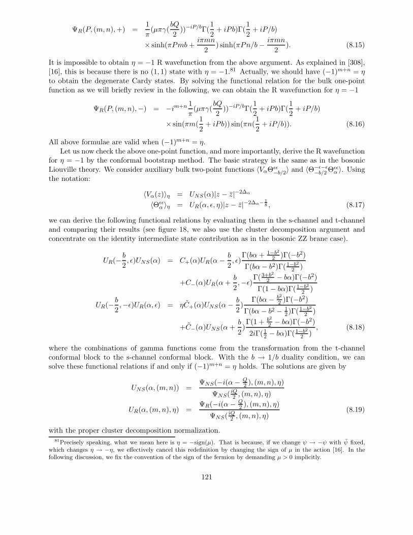
ΨR(P, (m,n),+) =1
π(µπγ(
bQ
2))−iP/bΓ(
1
2+ iP b)Γ(
1
2+ iP/b)
× sinh(πPmb+iπmn
2) sinh(πPn/b− iπmn
2). (8.15)
It is impossible to obtain η = −1 R wavefunction from the above argument. As explained in [308],[16], this is because there is no (1, 1) state with η = −1.81 Actually, we should have (−1)m+n = ηto obtain the degenerate Cardy states. By solving the functional relation for the bulk one-pointfunction as we will briefly review in the following, we can obtain the R wavefunction for η = −1
ΨR(P, (m,n),−) = −im+n 1
π(µπγ(
bQ
2))−iP/bΓ(
1
2+ iP b)Γ(
1
2+ iP/b)
× sin(πm(1
2+ iP b)) sin(πn(
1
2+ iP/b)). (8.16)
All above formulae are valid when (−1)m+n = η.Let us now check the above one-point function, and more importantly, derive the R wavefunction
for η = −1 by the conformal bootstrap method. The basic strategy is the same as in the bosonicLiouville theory. We consider auxiliary bulk two-point functions 〈VαΘǫǫ
−b/2〉 and 〈Θ−ǫ−ǫ−b/2 Θǫǫ
α 〉. Usingthe notation:
〈Vα(z)〉η = UNS(α)|z − z|−2∆α
〈Θǫǫα 〉η = UR(α, ǫ, η)|z − z|−2∆α− 1
8 , (8.17)
we can derive the following functional relations by evaluating them in the s-channel and t-channeland comparing their results (see figure 18, we also use the cluster decomposition argument andconcentrate on the identity intermediate state contribution as in the bosonic ZZ brane case).
UR(− b2, ǫ)UNS(α) = C+(α)UR(α− b
2, ǫ)
Γ(bα+ 1−b22 )Γ(−b2)
Γ(bα− b2)Γ(1−b22 )
+C−(α)UR(α+b
2,−ǫ)Γ(3+b2
2 − bα)Γ(−b2)Γ(1 − bα)Γ(1−b2
2 )
UR(− b2,−ǫ)UR(α, ǫ) = ηC+(α)UNS(α− b
2)
Γ(bα− b2
2 )Γ(−b2)Γ(bα− b2 − 1
2)Γ(1−b22 )
+C−(α)UNS(α+b
2)Γ(1 + b2
2 − bα)Γ(−b2)2iΓ(1
2 − bα)Γ(1−b22 )
, (8.18)
where the combinations of gamma functions come from the transformation from the t-channelconformal block to the s-channel conformal block. With the b → 1/b duality condition, we cansolve these functional relations if and only if (−1)m+n = η holds. The solutions are given by
UNS(α, (m,n)) =ΨNS(−i(α− Q
2 ), (m,n), η)
ΨNS( iQ2 , (m,n), η)
UR(α, (m,n), η) =ΨR(−i(α− Q
2 ), (m,n), η)
ΨNS( iQ2 , (m,n), η)(8.19)
with the proper cluster decomposition normalization.81Precisely speaking, what we mean here is η = −sign(µ). That is because, if we change ψ → −ψ with ψ fixed,
which changes η → −η, we effectively cancel this redefinition by changing the sign of µ in the action [16]. In thefollowing discussion, we fix the convention of the sign of the fermion by demanding µ > 0 implicitly.
121
Θ− b/2 Vα
Θ− b/2 + α or Θb/2 + α
Θ− b/2 Vα
1 1
Figure 18: The auxiliary two-point function can be calculated in two different ways.
Let us comment on the peculiar feature that only one type of branes is available as the super-symmetric ZZ brane. In the type 0 setup, we naively expect two kinds of branes — electric oneand magnetic one (in addition to the usual brane and its anti-brane). The nature of this doublingcomes from the fermionic boundary conditions ψL = ψR or ψL = −ψR. Actually, the two typesof D-branes are related by the transformation ψL → −ψL. However, this transformation is nolonger a symmetry once the Liouville superpotential is turned on. Therefore it is possible that onekind of brane becomes infinitely heavy and decouples from the theory. We will see the space-timeinterpretation of this result in the later section 9.
As in the bosonic theory, only (1, 1) brane has a semiclassical description as the Poincare diskmetric. In this case, the spectrum of c = 1 theory can be easily derived by suitability tensoringthe X,χ SCFT boundary states and the superghost boundary states. The spectrum depends onthe GSO projection (or the combination of the boundary states), but essentially the low energyspectrum consists of the tachyon with m2 = − 1
2α′ and massless (nondynamical) gauge boson (pro-vided they are not projected out). As in the bosonic theory, the movement of the ZZ-brane in theLiouville direction does not exist regardless of the GSO projection. We will see in section 9, thesebranes play a significant role in the holographic dual description of the super Liouville theory.
8.3 Super FZZT Brane
Next, we consider the quantum description of the super FZZT brane whose classical boundarycondition is given by (8.5). Our natural guess is that the non-degenerate state in the open channelis related to the spectrum of the string stretching between the super FZZT brane and the super(1, 1) ZZ brane as in the bosonic Liouville theory. By comparing its wavefunction and disk one-point function, we will obtain the precise relation between the weight of the non-degenerate stateand the boundary cosmological constant µB .
With this assumption we can write the following equations for the FZZT wavefunction Ψ(P, s, η)as
ΨNS(P, s, η)ΨNS(−P, (1, 1)), η) =1
2cos(2πPs)
ΨR(P, s, η)ΨR(−P, (1, 1), η) =1
2cos(2πPs). (8.20)
122
We can solve these equations from the knowledge of the (1, 1) wavefunctions. The solutions are
ΨNS(P, s, η) = − 1
2π(µπγ(
bQ
2))−iP/biPΓ(iP b)Γ(iP/b) cos(2πPs)
ΨR(P, s,+) =1
2π(µπγ(
bQ
2))−iP/bΓ(
1
2+ iP b)Γ(
1
2+ iP/b) cos(2πPs) (8.21)
As in the super ZZ brane case, we cannot obtain the R wavefunction for η = −1 by this methodbecause there is no (1, 1) state. However, using the functional relation for the one-point functionson the disk, we will obtain the η = −1 R wavefunction as
ΨR(P, s,−) =1
2π(µπγ(
bQ
2))−iP/bΓ(
1
2+ iP b)Γ(
1
2+ iP/b) sin(2πPs). (8.22)
It is important to note that the FZZT branes have indeed a second kind of brane unlike the ZZbranes. The magnetic and electric branes have different R wavefunctions, hence the different RRcharge.
Let us now check the above one-point function and derive the R wavefunction for η = −1 bythe conformal bootstrap method. The basic strategy is the same as in the ZZ case. We calculateauxiliary two-point functions 〈VαΘǫǫ
−b/2〉 and 〈Θ−ǫ−ǫ−b/2 Θǫǫ
α 〉 in two ways and compare the results. Theonly difference from the super ZZ case is that we calculate the bulk-boundary structure constantby the perturbation method
Θǫǫ−b/2 → r+ψB−b + r−B0
r− = −γbµB∫dx〈Θǫǫ
−b/2(i)ψBb(x)BQ(∞)〉free = ±√
2πbµBΓ(−b2)Γ(1 − b2
2)−2, (8.23)
where the last sign is somewhat subtle and we determine it from the consistency conditions. Thenthe functional relation becomes
r−UNS(α, s) = C+(α)UR(α− b
2, ǫ, s)
Γ(bα+ 1−b22 )Γ(−b2)
Γ(bα− b2)Γ(1−b22 )
+C−(α)UR(α+b
2,−ǫ, s)Γ(3+b2
2 − bα)Γ(−b2)Γ(1 − bα)Γ(1−b2
2 )
√2λ−2ir−UR(α, ǫ, s) = 2iηC+(α)UNS(α− b
2, s)
Γ(bα− b2
2 )Γ(−b2)√2Γ(bα− b2 − 1
2)Γ(1−b22 )
+C−(α)UNS(α+b
2, s)
Γ(1 + b2
2 − bα)Γ(−b2)√2Γ(1
2 − bα)Γ(1−b22 )
, (8.24)
where λ−2 is an ambiguity parameter from the four spin operator mixing we will not discuss here[308]. The consistency condition states it should be unity. Solving these equations with the usualduality constraint b → 1/b, we can obtain the one-point functions (8.21) and (8.22). Moreover,we have the following relation between the boundary parameter s and the boundary cosmologicalconstant µB:
µB =
(2µ
cos(πb2/2)
)1/2
cosh(πsb) (8.25)
for η = 1, and
µB =
(2µ
cos(πb2/2)
)1/2
sinh(πsb) (8.26)
123
for η = −1. It is interesting to note that the relation is different for the different choice of η.In the literature [308], another structure constant, namely the boundary two-point function
is derived, too. As in the bosonic Liouville theory, we expect that the logarithmic derivative oftwo-point functions is related to the density of states on the strip, which we can directly calculatefrom the boundary states derived above. Indeed it has been shown this is satisfied up to a divergentterm which needs a regularization (or we can consider the relative density of states as we have donein the bosonic case in section 5.1.2).
The derivation of the boundary two-point function is somewhat complicated but conceptuallystraightforward. As is the case with the bosonic Liouville theory, we make use of Teschner’s trickto calculate OPE of the degenerate boundary operator and a general boundary operator; then wesubstitute the reflection ansatz into the OPE (recall that the reflection amplitude is nothing but theboundary two-point function), and we obtain functional relations between these two-point functions.Solving these functional relations, we obtain the desired two-point functions. An interested readerwill consult the original paper for the further explanation and the actual calculation.
For the later purpose, we calculate here just one kind of density of states for illustration. Weconsider the partition function bounded by the following Cardy states
|FZZT, s,+〉 =
∫ ∞
−∞dP [ΨNS(−P, s,+)|P,NS,+〉 + ΨR(−P, s,+)|P,R,+〉] . (8.27)
The partition function becomes
Z =
∫ ∞
−∞dPΨNS(P, s,+)ΨNS(−P, s,+)χ+
P (NS)(τc) +1√2ΨR(P, s,+)ΨR(−P, s,+)χ+
P (R)(τc)
=
∫ ∞
−∞dP
∫ ∞
−∞dP ′e2πiPP
′(ΨNS(P, s,+)ΨNS(−P, s,+)χ+
P ′(NS)(τo)
+1√2ΨR(P, s,+)ΨR(−P, s,+)χ−
P ′(NS)(τo))
=1
2
∫ ∞
−∞dP ′
[ρ(P ′, s)(χ+
P ′(NS) + χ−P ′(NS))(τo) + ρ′(P ′, s)(χ+
P ′(NS) − χ−P ′(NS))(τo)
], (8.28)
where the open modular parameter τo is defined as τo = −1/τc, and the density of states here isgiven by
ρ(P ′, s) =
∫ ∞
−∞dP
e2πiPP′cosh(πQP ) cos(2πsP ) cos(2πsP )
sinh(2πbP ) sinh(2πP/b)
ρ′(P ′, s) =
∫ ∞
−∞dP
e2πiPP′cosh(π(b− b−1)P ) cos(2πsP ) cos(2πsP )
sinh(2πbP ) sinh(2πP/b). (8.29)
These density of states are divergent, so we must impose an infrared regularization. It is interestingto note that the R contribution to the density of states is very small because the P → 0 divergencemostly comes from the NS-NS exchange. As a consequence, the open GSO projection is notimposed in this spectrum as opposed to the naive free field expectation.82 Note, in addition, eventhe infrared bulk singular behavior P → 0 which corresponds to the logµ term is not reproducedwith this wavefunction.
82In the free field case, both NS wavefunction and R wavefunction behave as δ(P ), so ρ′(P ) actually vanishes andthe open GSO projection is imposed for this Cardy state. Of course, in the free field, if we consider an “unstable”brane whose wavefunction is only NS, the GSO projection is not imposed.
124

8.4 Literature Guide for Section 8
On the structure constants of the boundary super Liouville theory, the bulk one-point functionhas been studied in [308], [325], and the boundary two-point function has been studied in [308].The remaining structure constants which have not been obtained so far are the bulk boundarytwo-point function and the boundary three-point function. These cannot be obtained from themodular bootstrap and require a thorough investigation of the boundary bootstrap, which seemsto be a hard work.
9 Matrix Model Dual
In this section, we consider the matrix model dual of the supersymmetric Liouville theory whosecontinuum properties have been discussed in section 7. The fundamental observation behind thisduality lies in the holographic perspective we have discussed in section 6.1. We will construct thematrix model duals from the tachyon dynamics on the unstable ZZ branes. The organization ofthis section is as follows.
In section 9.1, we review the c = 1 matrix quantum mechanics. In subsection 9.1.1, we recallthe possible branes in the two dimensional type 0 noncritical string theory. In subsection 9.1.2,we discuss the dual matrix model for the type 0B theory. In subsection 9.1.3, we discuss the dualmatrix model for the type 0A theory. We will see that the matrix model reproduces the continuumLiouville results in some examples. At the same time, we obtain the matrix model descriptionwhich cannot be handled from the world sheet NS-R formulation, e.g. the theory with the fluxbackground.
In section 9.2, we review the c = 0 matrix models. In subsection 9.2.1, we discuss the unitarymatrix model which is the dual matrix model for the type 0B theory. In subsection 9.2.2, we discussthe complex matrix model which is the dual matrix model for the type 0A theory. The comparisonwith the continuum super Liouville theory will be done in subsection 9.2.3.
9.1 c = 1 Matrix Quantum Mechanics
In this section, we focus on the c = 1 super Liouville theory whose dual matrix theory should be acertain matrix quantum mechanics. First, we review the brane contents in the c = 1 super Liouvilletheory and then we present the dual matrix model proposal made in [174], [16].
9.1.1 Branes in c = 1 theory
We have briefly reviewed the space-time spectrum of the type 0A and type 0B theory in section7.3, so let us now list the D-branes in this setup from the space-time point of view.
For the type 0B theory, we have two kinds of massless scalar fields (NS-NS and R-R) in thespectrum. The closed GSO projection determines the allowed boundary states in the theory. Inthe type 0B theory, any D-brane allows NS boundary states, but only the odd space dimensionbranes allow R boundary states. Therefore, for the “stable brane” we have only the D1-branein the Minkowski signature.83 It is charged under the R-R two-form which does not propagate.Therefore, we should consider only D1-D1 pair for the R-R tadpole cancellation (NS-NS tadpolecan be canceled by the Fischler-Susskind mechanism if one wants). Here, by antibrane D, we mean
83In the Minkowski signature, we only consider the time-like brane, i.e. we take the Neumann boundary conditionfor X.
125

the brane whose R wavefunction is reversed:
|D-brane,±〉 = |NS,±〉 + |R,±〉|D-brane,±〉 = |NS,±〉 − |R,±〉. (9.1)
Therefore there are four kinds of brane. We distinguish ± by calling electric and magnetic respec-tively. Note that in the super Liouville theory they are actually different branes.
However, there is a small subtlety here. The natural candidate for this brane is the FZZT ⊗X Neumann brane in the exact super Liouville description. We recall that there are two kindsof FZZT R wavefunction corresponding to η = ±, and whose cylinder divergence from the R-Rexchange is much weaker than the usual NS-NS exchange divergence. Particularly, for η = −,the R-R tadpole cylinder diagram actually converges. The author is not quite sure whether theR-R tadpole (non)divergence should be canceled in this case or not. In addition, by saying “stablebrane”, we usually mean that the (massless) tachyon on them are projected out by the open GSOprojection. As we have seen in the last section, however, the GSO projection on them actually doesnot work because of the wavefunction difference for NS sector and R sector even if we take µB = 0.The true meaning of this observation is unclear to the author. Also there is a subtlety concerningthe allowed D1-brane. See appendix B.5 for a further discussion on the discrepancy between thefree field observation and the super Liouville treatment.
Now let us go on to the unstable brane whose dynamics we expect to be the dual description ofthe bulk system. We have D0-brane in the type 0B theory whose boundary state is given by the NS(1,1) ZZ brane (no R wavefunction). With N such branes, we have U(N) adjoint tachyons whosemass is m2 = − 1
2α′ . The conjecture made in [174], [16] is that the matrix quantum mechanicsrealized by these tachyons in the double scaling limit provides the holographic dual description ofthe type 0B super Liouville theory.
For the type 0A, we have one NS-NS tachyon and two R-R nondynamical vectors as the closedstring spectrum. The closed GSO projection determines allowed branes in the type 0A theory. Forstable branes, we have a D0-brane which is the source of the R-R one-form. Because of the GSOprojection (recall that for the ZZ brane, the open GSO projection works properly), we have toconsider D0-D0 pair to have nontrivial tachyon dynamics. The proposal made in [16] is that thequantum mechanics on N D0 branes and (N + q) D0 antibranes provides the holographic dual ofthe super Liouville theory with q background R-R charge installed. Note that the ZZ brane in thiscase actually has one kind (no magnetic one) because the (1, 1) ZZ brane necessarily has η = +.
In the type 0A theory, we also have the “unstable” D1-brane whose property is similar to theD1-D1 pair in the 0B case. The natural extension of the bosonic Liouville theory (6.2) leads to thematrix vector theory for this case. The study on this matrix-vector model, however, is only limitedup to date.
9.1.2 Type 0B matrix quantum mechanics
The type 0B matrix quantum mechanics is proposed as the dynamics of the tachyon matrix onthe N D0-branes. The mass of the tachyon is given by m2 = −1/2α′ and more importantly, thepotential for the tachyon is symmetric under M → −M . The symmetry under M → −M comesfrom the world sheet symmetry (−1)FL , where FL is the space-time fermion number, and the bothsides of the Fermi sea should be filled with. Therefore, the matrix quantum mechanics for the type0B theory is expected to be stable as opposed to the bosonic Liouville theory which is believed tobe nonperturbatively unstable. In this way, we are naturally led to the two-cut Hermitian matrixmodel.
S =
∫ ∞
−∞dtTr
(1
2(DtM)2 + V (M)
)(9.2)
126
In the double scaling limit, which corresponds to the Maldacena limit in the AdS/CFT language,we consider the following inverted harmonic oscillator potential
V (λ) = − 1
4α′λ2, (9.3)
where we have diagonalized the Hermitian matrix. In the following we will check the proposal bycomparing two quantities, which can be also derived in the continuum super Liouville formalism,the finite temperature free energy and the scattering amplitudes.
The finite temperature free energy (or the string partition function with compactified EuclideanX) can be obtained very easily [16] once we know the result for the matrix dual of the bosonicLiouville theory. The difference from the bosonic Liouville theory is simply the tachyon mass− 1α′ → − 1
2α′ and the final division by two. Thus we can immediately borrow the result for thebosonic theory which is summarized in the Gross-Klebanov formula (3.97) and replace α′ → 2α′
and not divide by two84:
∂ρ
∂µ=
√2α′
πµIm
∫ ∞
0dte−it
t/(2βµ√
2α′)
sinh[t/2βµ√
2α′]
t/(2βµR)
sinh[t/2βµR], (9.4)
where the partition function itself is given by
∂2Z
∂µ2= ρ. (9.5)
For example, the torus partition function can be calculated as
Z = − log µ
12
(R√2α′ +
√2α′
R
), (9.6)
which reproduces the continuum result (7.35).Now let us go on to the comparison of the S matrix. The important point we should consider
first is the leg pole factor which is the momentum dependent, hence non-local, wavefunction renor-malization factor connecting the collective field operators with the spacetime tachyon operators.As in the bosonic Liouville theory, this factor can be calculated from the decaying amplitude of theunstable (ZZ) D0-brane.
For the time part, we use the following boundary action [326], [174], [16]:
δS = λ
∫
∂Σηψe
12X0, (9.7)
where η is the anticommuting boundary fermion with η2 = 1. The NS-NS tachyon amplitude forthe X0 part is given by
At = 〈eiEX0〉 = − 1√2π
(√
2λπ)−2iE π
sinh(πE). (9.8)
On the other hand, the NS-NS one-point function for the (1, 1) ZZ brane is given by (see (8.15)),
Aφ = 〈e(iP+1)φ〉 = −i(µr)−iPΓ(iP ) sinh(πP )
Γ(−iP )(9.9)
84As in the bosonic Liouville theory, since the adjoint tachyon is gauged, only the singlet representation contributeto the thermal path integral.
127
where we have introduced a renormalized cosmological constant µr = µ0γ(1)π. With the mass-shellcondition E = P , we have
ANS = AtAφ = µ−iPr
Γ(iP )
Γ(−iP )e−iP log(2π2λ2), (9.10)
which yields the NS-NS leg pole factor eiδNS times the time delay factor e−iP log(2π2λ2). We cancheck that the tachyon scattering in the continuum super Liouville formalism factorizes with thisfactor attached to every external leg as in the bosonic Liouville theory [110]. For the R-R sector,the only difference in the X0 part is the factor cosh(πE) instead of sinh(πE). With the (1, 1) ZZamplitude for the R-R wavefunction, we have
AR = µ−iPr
Γ(12 + iP )
Γ(12 − iP )
e−iP log(2π2λ2), (9.11)
which is known to provide the correct leg pole factor for the R-R field.85
The matrix model for the type 0B theory fills both sides of the Fermi sea. Therefore, the smalldisturbances of the Fermi sea on the left side TL(k) and the right side TR(k) are perturbativelyindependent. Actually the same thing holds in the super Liouville calculation on the sphere. Thisnaturally leads to the following identification:
T (k) = eiδNS (TR(k) + TL(k))V (k) = eiδR (TR(k) − TL(k)) . (9.12)
We can also see that the S matrix for the odd number V (k) insertion is zero. In the original matrixmodel language, the corresponding vertex operator is proposed to be [174]86
T (q) ∼ PNS(q) = liml→0
l−|q|/2ONS(q, l)
V (q) ∼ PR(q) = liml→0
l(−|q|+1)/2OR(q, l), (9.13)
where the NS and R puncture operators are
ONS(q, l) =
∫dxeiqxTr[e−lM(x)2 ]
OR(q, l) =
∫dxeiqxTr[M(x)e−lM(x)2 ]. (9.14)
Now, the central problem is whether this vertex shows the correct leg pole factor after fermionizationand rebosonization as in the bosonic Liouville theory which has been treated in section 3.2.
Let us consider the NS operator first. The bosonization procedure is just the same as in thebosonic theory87, so we write the puncture operators as
ONS(q, l) = i
∫dkF (k, l)kS(q, k), (9.15)
85This can be obtained by analyzing the R-R correlator when the Liouville momentum is conserved up to pertur-bative insertions as in the bosonic Liouville theory in section 3.2.2. The reason why zero momentum R-R field doesnot decouple is that the R-R zero-mode minisuperspace wave equation (Dirac equation) has a normalizable solutionfor the zero energy as opposed to the NS-NS sector. At the same time, we should recall that the (−1/2,−1/2) vertexconsidered here is associated with the R-R field strength rather than the potential itself.
86Following [174], we use the convention α′ = 1/2 here in order to borrow the bosonic theory formulae in section3. In the end of the calculation we set p,E → 2p, 2E to obtain the α′ = 2 results.
87Strictly speaking, the bosonization deals just the half part of the Fermi surface, so we should have two kinds ofbosonization at the same time. For the NS part, the diagonal matrix is implicitly suppressed in the following formula.
128

TL TR
Figure 19: The matrix model dual of the type-0B is given by the double scaling matrix quantummechanics with both sides of the potential filled.
where
F (k, l) =
∫dτe−ly
2(τ) cos(kτ). (9.16)
Evaluating F (k, l) with the classical trajectory y(τ) =√
2µ cosh(τ), we obtain
F (k, l) =e−lµ
2Kik/2(lµ). (9.17)
In the small l limit, we find
F (k, l) ∼ π
4 sin( ikπ2 )
((lµ/2)−ik/2
1
Γ(−ik/2 + 1)− (lµ/2)ik/2
1
Γ(ik/2 + 1)
). (9.18)
As in the bosonic Liouville theory, we should add this factor to every external line of the EuclideanFeynman diagram. Picking up the pole for the integration over k, we obtain the leg factor
(lµ/2)|q|/2Γ(−|q|/2). (9.19)
Further multiplying by 1/Γ(|q|/2), which yields the precise operator mapping from the super Liou-ville theory to the matrix puncture operator, we have reproduced the full leg pole factor (9.10) forthe S bosonic theory
µ−iPΓ(iP )
Γ(−iP ), (9.20)
where we have translated the final result into the α′ = 2 notation.Now let us consider the RR sector. The corresponding wavefunction for the bosonization is
given by
F (k, l) =
∫dτye−ly
2cos(kτ). (9.21)
For y =√
2µ cosh τ , we find
F (k, l) =1
2
õ
2e−lµ
(K(1+ik)/2(lµ) +K(−1+ik)/2(lµ)
). (9.22)
129
In the small l limit, we have
F (k, l) =
õ
2(lµ/2)−1/2
[π
4 sin((ik + 1)π/2)(lµ/2)−ik/2
1
Γ((−ik − 1)/2 + 1)+ cc
], (9.23)
which yields the following external leg factor for every external line of S bosonõ
2(lµ/2)(|q|−1)/2Γ((1 − |q|)/2). (9.24)
Returning to the Lorentzian signature and multiplying 1/Γ(1/2− iP ), we have the correct leg polefactor (9.11)
µ−iPΓ(1/2 + iP )
Γ(1/2 − iP ). (9.25)
They are associated with the S boson scattering amplitude which decouples in the zero momentumlimit. To relate this amplitude with the continuum calculation of the (−1/2,−1/2) picture R-Rvertex insertion, further division by 2iP is needed because the string calculation deals with thefield strength.
9.1.3 Type 0A matrix quantum mechanics
The matrix dual for the type 0A theory can be obtained similarly from the double scaling limit ofthe matrix quantum mechanics on the unstable N D0 branes and (N+q) D0 antibranes system [16].The open string theory on these branes is from the tachyon which transforms as the U(N)×U(N+q)bifundamental. The Lagrangian (in the double scaling limit) is given by
L = Tr
[(DtT )†DtT +
1
2α′T†T
], (9.26)
where T is an N × (N + q) complex matrix.To solve this system, it is convenient to diagonalize T . However, the special care is needed
because it is not an Hermitian matrix as has been exclusively studied so far. For the time being,let us concentrate on the q = 0 case. Recall that any N ×N complex matrix T can be decomposedas
T = V xW †, (9.27)
where V and W are unitary matrices and x is a real and nonnegative diagonal matrix. The changeof variables to V, x,W needs a Jacobian [327], [328], [329]. To obtain this Jacobian J , we use thefollowing trick (see e.g. [328]). First, we write the infinitesimal variation of (9.27) as
V †δTW = δSx− xδM + δx, (9.28)
where δS = V †δV and δM = W †δW . On the other hand, with the flat measure for δT, δM andδS, we have
Const =
∫d(δT ) exp
[−TrδT †δT
]
=
∫d(δS)d(δM)dN (δx)J exp [−Tr(xδS − δMx− δx)(δSx − xδM + δx)] . (9.29)
Making the linear substitution
δSαβ → δSαβ +2δMαβxαxβx2α + x2
β
, (9.30)
130

we end up with
TrδT †δT =∑
αβ
((x2α + x2
β)δSαβδS∗αβ + δMαβδM
∗αβ
(x2α − x2
β)2
(x2α + x2
β)
)+∑
α
δx2α. (9.31)
Carrying out the Gaussian integration (9.29), we have
J = const∏
α
xα∏
α<β
(x2α − x2
β)2 (9.32)
as the Jacobian. Note that the symmetric part of δM is the redundant variable.Then we can write down the Schrodinger equation for the diagonal elements via Pauli’s method.
Setting χ =∏i<j(x
2i − x2
j )ψ(x), we obtain
(− 1
2xi
∂
∂xixi
∂
∂xi− 1
4α′x2i
)χ = Eχ. (9.33)
The simple generalization for the q 6= 0 yields
(− 1
2x1+2qi
∂
∂xix1+2qi
∂
∂xi− 1
4α′ x2i
)x−qχ = Ex−qχ. (9.34)
Or equivalently, (− 1
2xi
∂
∂xixi
∂
∂xi+
q2
2x2i
− 1
4α′x2i
)χ = Eχ. (9.35)
This quantum mechanical problem is exactly solvable and the finite temperature free energy iscalculable.88 In [16], it is given by
∂ρ
∂µ=
√α′/2
πµIm
∫ ∞
0dte−it
t/(2βµ√α′/2)
sinh[t/(2βµ√α′/2)]
t/2βµR
sinh[t/2βµR]e−qt/(2β|µ|
√α′/2). (9.36)
The one-loop contribution becomes
Z = log µ
[− 1
24
(4
R√2α′ +
√2α′
R
)+
1
2q2
R√2α′
](9.37)
The first term reproduces the continuum results (7.35) and the second term which is proportionalto q2 yields the background charge contribution to the partition function as was studied in [16] fromthe space-time point of view. To derive the expression (9.36), we need to know the zero energydensity of states as in the bosonic Liouville theory (see section 3.2). The zero energy density ofstates is easily obtained by calculating the phase shift of the scattering event
ρ(e) =1
2π
∂δ(e)
∂e. (9.38)
See section 4.2 for the explanation of this formula. By the suitable change of variable, the phaseshift can be exactly calculable for the Hamiltonian (9.34). An interested reader should consultappendix B of [16].
88To see this explicitly, it is convenient to redefine ψ = x1/2χ.
131

Figure 20: The matrix model dual of the type-0A is given by the complex rectangular matrixquantum mechanics. In the eigenvalue basis, the potential is slightly deformed.
9.2 c = 0 Matrix Model
In [161], the matrix model dual for the c = 0 (or more generally, some classes of the superconformalc < 1 matter coupled to the world sheet supergravity) string theory is proposed. The analogy to thelast section’s argument suggests that the type 0A theory is dual to the double scaling limit of theHermitian matrix models with two-cut eigenvalue distribution (or the unitary matrix model) andthe type 0B theory is dual to the rectangular complex matrix model. In this section, we exclusivelydeal with the simplest c = 0 model, namely the pure 2D supergravity theory. For the multi criticalmatrix model which is related to the c < 1 theory coupled to minimal matters, we refer to [161],[330].
9.2.1 Unitary matrix model
The double scaling limit of the unitary matrix model is first solved in [331, 332]. First, we reviewits solution for the simplest case. The string partition function is given by
eZ =
∫dU exp
(−Nγ
TrV (U + U †)
). (9.39)
where U is unitary and the simplest potential which we consider here is given by V (x) = x. We
diagonalize the unitary matrix as V†UV = diag(eα1 , · · · eαN ). With these variables, the measure
becomesdU =
∏
i
dαi∆(α)∆(α), (9.40)
132

where the Jacobian is given by
∆ =∏
i<j
(exp(iαi) − exp(iαj)) . (9.41)
Using the notation zi = eiαi , we can write the matrix integral (9.39) as
eZ =
∫dα∆(α)∆(α) exp
[−Nγ
∑
i
V (zi + z−1i )
]. (9.42)
As we have done in the Hermitian matrix model in section 3.1, we make use of the orthogonalpolynomial technique. The orthogonal polynomials in this case are normalized as
∫ 2π
0dµpn(z)pm(z−1) = hnδn,m, (9.43)
where dµ ≡ dz2πiz exp(−V (z + z−1)) and pm(z) = zm + · · · + Rm−1. From the definition, we can
derive the following recursion relation
pn+1(z) = zpn(z) +Rnznpn(z
−1). (9.44)
By multiplying pn or pn+1 and integrating over dµ, we can easily obtain the relation hn+1/hn =1 − R2
n. Then as in the Hermitian matrix model (see section 3.1.1), we can rewrite the partitionfunction as
eZ ∝ N !∏
i
(1 −Ri−1)N−i. (9.45)
Therefore the remaining task is to obtain the expression for R in the double scaling limit. In thislimit the partition function is given by −Z ′′ = f2 where f is proportional to R. Just as we haveobtained (3.15), we can use the partial integration to obtain
(n+ 1)(hn+1 − hn) = −∫dµV ′(z + z−1)(1 − 1/z2)pn+1(z)pn(z
−1). (9.46)
With the simplest potential V ′ = Nγ , we obtain the discrete “string equation”:
γ
N(n+ 1)R2
n = Rn(Rn+1 +Rn−1)(1 −R2n). (9.47)
From this expression, we can see that the critical point is given by γ = 2, nN = 1 and Rn = 0. In
order to take the double scaling limit, we introduce the following scaling ansatz:
ξ =n
Ny = (2 − γ)N2/3
z = (2 − γξ)N2/3
f = N1/3R. (9.48)
Fixing y and taking the N → ∞, γ → 2 limit of (9.47), we can obtain89 the following continuumstring equation
−2zf + 2f3 = ∂2zf, (9.49)
89The calculation is the same as has been done in section 3.1.1.
133

which is what is called the Painleve II equation with a rescaling of y by a numerical factor.90 Thesolution of the equation yields the partition function after we integrate it twice.
The slight extension of the model has been considered in [161] (see also [334]). Without aderivation (see [161]), we just assume the following extended string equation:
f ′′ − 1
2f3 +
1
2zf +
q2
f3= 0. (9.50)
We would like to see its consequence and the physical meaning of the q2 term in the following.The perturbative solution of (9.50) 91 for large positive z is given by
u(z) = f2(z)/4 =z
4+
(q2 − 1
4
)[1
2z2+
(q2 − 9
4
)[− 2
z5+ · · ·
]], (9.51)
whereas, for the large negative z, the solution is given by
u(z) = f2(z)/4 =|q|
√2
4|z|1/2 − q2
4|z|2 +5|q|(1 + 4q2)
√2
64|z|7/2 − q2(7 + 8q2)
8|z|5 · · · , (9.52)
The important point is that u(z) is not an analytic function of q. This leads the authors of [161]to the conclusion that for z < 0, the physical R-R vertex which turns on the q perturbation doesnot exist. We will see in section 9.2.3 its explanation from the super Liouville theory.
The physical interpretation of this (second derivative of the) partition function is as follows.First, we note that the world sheet genus expansion is given by the term proportional to |z|1−3(g+b/2)
with g handles and b boundaries. From this (and the analytic property of q dependence which wehave seen above), we can guess the physical interpretation of the q deformation. When z ∼ µ > 0,we have the closed string theory, where the R-R flux operator is inserted which produces the qcontribution. On the other hand, when z ∼ µ < 0, we have the open string theory where |q| yieldsthe number of branes. With this interpretation, it is natural to consider that q is quantized.
As is emphasized in [161], we have actually the smooth description when we change µ fromthe large negative value to the large positive value. This is because the original matrix model (orthe extended action) is smooth in the change of z as long as q > 0. However, the perturbativedescription is very different — on one hand we have the open string theory, and on the other handwe have the closed string theory with the R-R flux. This suggests the geometric transition typeof duality [77], [335], [336], [83]. We have encountered the exact description of the sophisticatedduality of the string theory in the Liouville - matrix model setup again!
While the last statement holds perturbatively in q, the large q ’t Hooft limit also has beenstudied in [161]. Here by the ’t Hooft limit, we mean q → ∞ and z → ±∞ with t = q−2/3z fixed.In this limit, the second derivative of the partition function behaves as
v(t) =
√2
|t|1/2 − 1
|t|2 +5√
2
4|t|7/5 + · · · , t < 0
90This equation can be also obtained from the double cut Hermitian matrix model as it should be. The applicationto the gauge theory in the context of the Dijkgraaf-Vafa proposal has been recently studied in [333]. However weshould think seriously the existence of poles in the solution of the Painleve equation in this case. This is becausethe Dijkgraaf-Vafa matrix model is a holomorphic matrix model, i.e. the coefficient of the potential is complex innature. The physical meaning of this kind of singularity in the double scaling limit of the prepotential (which shouldcorrespond to the nonperturbative completion of the nonperturbative graviphoton correction) is not clear so far.Perhaps, there may be other branches of solution which is regular.
91Since z is related to the cosmological constant, hence the string coupling, this is the weak coupling expansion.
134
v(t) = t+2
t2− 8
t5+
56
t8− · · · t > 0. (9.53)
This expression has the obvious geometric transition type interpretation. For negative t, we haveD-branes and the ’t Hooft limit is given by the planer graph. For positive t, we have no D-branes,but instead we have R-R flux background. It is important to note that the latter expansion is basedon the R-R flux t−3 expansion and not the world sheet (loop) expansion.
9.2.2 Complex matrix model
The natural candidate for the matrix model dual of the type 0A c = 0 string theory, which isequivalent to the 2D pure supergravity, is the double scaling limit of the rectangular complexmatrix model. In this subsection, we review its solution and the physical meaning of the result[161].
The string partition function is given by the following matrix integral [337], [338, 339], [340],[327], [161]:
eZ =
∫dMdM † exp
[−NγV (MM †)
], (9.54)
where M is given by the complex N × (N + q) complex matrix. The diagonalization of this matrixand the associated Jacobian have been reviewed in section 9.1.3. Setting y = x2, we have
eZ =
N∏
i=1
∫ ∞
0dyiy
qi e
−NγV (yi)∆(y)2, (9.55)
where ∆(y) =∏i<j(yi−yj) is the usual Vandermonde determinant. Then we define the orthogonal
polynomials Pn as ∫dµPnPm =
∫ ∞
0dyyqe
−NγVPnPm = δnm, (9.56)
which begins like Pn = yn + · · · . For simplicity, we show the calculation for the q = 0 case in thefollowing. First, from the definition of the orthogonal polynomials, we have the recursion relation
yPn = Pn+1 + snPn + rnPn−1 (9.57)
with rn = hn/hn−1. Next, by using the partial integration we can derive the following relation:
h−1n
∫dµPnV
′Pn = Ωn
h−1n−1
∫dµPn−1V
′Pn = xn + Ωn, (9.58)
where we have introduced xn, Ωn and Ωn as
xn ≡ γn
N
Ωn ≡ γ
N
Pn(0)2
hne−
NγV (0)
Ωn ≡ γ
N
Pn−1(0)Pn(0)
hn−1e−
NγV (0). (9.59)
From its definition, we immediately obtain
rnΩnΩn−1 = Ω2n. (9.60)
135
In addition, by multiplying V ′Pn to (9.57) and integrating over dµ, we have
Ωn + Ωn+1 = −snΩn. (9.61)
With the simplest potential V (y) = −y + y2
2 , which corresponds to the pure supergravity theory,we have the following string equations:
rn − xn = Ωn
Ωn + Ωn+1 = −(Ωn + 1)Ωn
rnΩnΩn−1 = Ωn2. (9.62)
As has been shown in the literature [161], the double scaling ansatz is given by
r =1
4− ǫ(u+ z/2), x =
1
4− ǫz, Ω = ǫΩ, Ω = −ǫR, N = γǫ−3/2. (9.63)
With these variables, the continuum limit of the string equations and the partition function become
0 = 8uR2 − 1
2RR′′ +
1
4(R′)2
R = u− z/2Z ′′ = −4u. (9.64)
The extension for nonzero q is straightforward, and the result is
q2
4= 8uR2 − 1
2RR′′ +
1
4(R′)2
R = u− z/2Z ′′ = −4u. (9.65)
It is convenient to rescale the parameter as u = 25/3u, z = 22/3z and R = 25/3R. Substitutingu(z) = f(z)2 + z, we have
∂2zf − f3 − zf +
q2
f3= 0. (9.66)
Surprisingly, up to the trivial rescaling and important sign in front of z, this is just the PainleveII equation derived in the last subsection for the matrix model dual for the type 0B theory. Thisleads the authors of [161] to the conjecture that the c = 0 super Liouville theory has the duality:the type 0A with µ > 0 is dual to the type 0B with µ < 0 and the type 0A with µ < 0 is dualto the type 0B with µ > 0. Typically, the unitary matrix model and the complex matrix modelhave a corresponding model with each other. Therefore we expect the similar duality holds for thegeneral c < 1 model.
At the same time, this duality strongly suggests the D-brane like contribution of the quantity qin the partition function because we regard the double scaling limit of the complex matrix theoryas the super Liouville theory with q extra D-branes background.
9.2.3 Comparison with super Liouville theory
So far, we have solved the unitary and complex matrix model without any reference to the underlingsuper Liouville theory. Here, we list some of the comparisons made in [161] which confirms thematrix model proposal for the super Liouville theory.
136
• The first point is the physical state for the one dimensional noncritical fermionic string theory.To describe the theory in the super Liouville language, we take Q = 3√
2and b = 1√
2. The
cosmological constant scales as µ3(2−2g)/2 in the partition function. The physical vertexoperators are as follows. For the NS-NS sector, we have ebφ in the (−1,−1) picture. Forthe R-R sector, the naive free field guess is that we have V± = σ±eQφ/2 in the (−1/2,−1/2)picture.92 In the nonzero energy sector, the both ± vertices appear, but in the zero energysector considered here, the one of the zero-mode wavefunction does not damp in the φ→ ∞region in the minisuperspace approximation. The behavior is correlated with the sign of µ.Thus for µ < 0, only V+ is acceptable while for µ > 0 only V− is acceptable, which meansthat in the type 0A theory there is one R-R operator for µ < 0 and no operator for µ > 0. Inthe type 0B, the situation is reversed. This fact is compatible with the claim that µ → −µexchanges 0A and 0B theory.
• In [161], the connection between the FZZT brane and the matrix resolvent has been studied.The dependence of the boundary and bulk cosmological constant of the FZZT brane revealsthat the η = −1 brane in the type 0B theory is related to the resolvent of the two cut matrixmodel. On the other hand, the FZZT brane with η = 1 is related to the resolvent of thecomplex matrix model. See also [67] for the interpretation of the ZZ and FZZT branes inthe super Liouville theory coupled to the super minimal models from the Riemann surfaceviewpoint.
• The torus partition functions have been calculated and compared with the matrix modelprediction [161]. Although the odd spin structure partition function is difficult to evaluate,the other calculable partition functions match with each other.
9.3 Literature Guide for Section 9
The matrix quantum mechanics dual of the c = 1 super Liouville theory (two dimensional fermionicstring theory) has been proposed in [174], [16]. In addition to the check we have reviewed in themain text, the ground ring structure has been studied in [16]. The earlier references on the BRSTcohomology and the ground ring for the two dimensional fermionic string theory include [341], [342],[343], [344].
The earlier studies on the c < 1 unitary matrix model (or the double cut Hermitian matrixmodel) can be found in [345], [331], [338], [332], [346], [347], [348], [349], [334], some of which (e.g.[348]) connect the multiple critical behavior with the Zakharov-Shabat hierarchy. Since we havefocused on the simplest example, we have not emphasized the point in the main text, but thisviewpoint is useful when we extend the string equation to the multicritical theory which is relatedto the super Liouville theory coupled to the super minimal model.
On the other hand, the earlier studies on the complex rectangular matrix model can be foundin [339, 350], [337], [340]. More recently, extending the type 0A string interpretation of this modelproposed in [161], [330] has argued the more general gravitational coupling to the super minimalmodels and has studied particularly the tricritical Ising model coupled to the world sheet super-gravity (super Liouville theory) in detail.
92We have used the two dimensional diagonal representation here. See appendix B.5 for the zero-mode algebra.The dimension of the operator is obtained in the following manner: the ghost and superghost contribute − 5
8and the
spin field contribute 116
, finally the Liouville part is given by 12
Q2(Q− Q
2) = 9
16, hence the total dimension is zero.
137
10 Applications
In this section we review various applications of the N = 1 super Liouville theory and its matrixmodel dual. The organization of this section is as follows.
In section 10.1, we discuss the scattering amplitudes in the R-R background, which cannot beeasily obtained from the world sheet theory. In section 10.2, the unitarity of the type 0B S matrixwill be discussed, where we will find that the θ vacua like degeneration emerges. In section 10.3,the hole interpretation of the matrix model from the boundary states is reviewed. The hole statesare interpreted as the boundary states with an extra minus sign which has a negative energy ifthe plus sign is assigned. In section 10.4, we review the nonperturbative generation of the R-Rpotential, which stabilizes the moduli.
10.1 Scattering in R-R Background
Matrix model dual prediction enables us to calculate the scattering amplitudes in an R-R back-ground for the type 0A theory [351]. The type 0A matrix model has one integer parameter q whichrepresents the number of extra stable D0-branes (hence, the remaining R-R flux in the double scal-ing limit closed theory). After the diagonalization of the complex rectangular matrix, the effectivepotential for the eigenvalue becomes
V (λ) = − λ2
2α2+q2 − 1
4
2λ2, (10.1)
where we have introduced α =√
2α′ to relate the potential to the bosonic convention. It isimportant to note that the eigenvalue is restricted to λ > 0.
By the way, this potential reminds us of the bosonic Liouville theory with an unstable D-braneon top of the potential (see section 6.4), where we have the same potential. There we have observedthat the scattering amplitudes are not modified at the tree level or the disk level. Since the potentialis the same, we expect the same result.
The only information needed to obtain the S matrix in the MPR formalism (see section 3.2.3)is just the reflection amplitude of the potential (10.1). Since the theory is solvable quantummechanically (see section 9.1.3 or [352]), we can find that the amplitude is given by
R(p) =
∣∣∣∣∣q2 − 1
4 + α2µ2
4
∣∣∣∣∣
−α|p|/2Γ(1
2 + |q|2 − i
2αµ+ 12α|p|)
Γ(12 + |q|
2 + i2αµ− 1
2α|p|). (10.2)
(We have considered the Euclidean amplitudes here. To obtain the Minkowski amplitudes we simplysubstitute |p| → iω). In the following we set α = 1.
Following the MPR rule, we can calculate any S matrix via the reflection amplitude (10.2). Forexample, the three-point amplitude is given by
A3(p1, p2;−p) = −i(∫ p
p1
R(p − x)R∗(x)dx+
∫ p
p2
R(p− x)R∗(x)dx−∫ p
0R(p− x)R∗(x)dx
),
(10.3)where we have suppressed the momentum conservation factor δ(p1 + p2 = p). The one-loop resultis given by
A3(p1, p2;−p) =−p1p2p
µ
(1 − 1
24(p4 − 2p3(p1 + 2) + 2p2(p2
1 + 3p1 + 2)
− p(6p21 + 4p1 − 1) + 4(p2
1 − 2) + 24q2)µ−2 + · · ·). (10.4)
138
Usually, the scattering amplitudes in the R-R background is difficult to calculate because thesensible R-NS formulation in the R-R background perturbation theory is limited. The world sheetderivation of these amplitudes is a challenging problem.93
With the exact MPR formula, we can calculate the scattering amplitudes in various limits. Forexample, in [351], the following two limits have been considered. The strong field limit is the limitwhere we fix q = fµ and expand in 1/µ. The three-body S matrix becomes
A3(p1, p2,−p) =−p1p2p
(1 + f2)µ+ · · · , (10.5)
It is interesting to observe that the renormalization
µ→ µ = (1 + f2)µ, (10.6)
yields the same tree level amplitudes for any correlation function (but not for the loop correction).The dual string limit is defined as follows. We set g′s = 1/q and q′ = µ with fixed f ′ = 1
f . Thenthe three-point function becomes
A3(p1, p2;−p) = −f ′g′sp1p2p+ · · · (10.7)
and other amplitudes also admit a g′s expansion under the dual R-R flux f ′. The nature of thisdual theory is not well-known.94
Actually, the more radical limit is possible as long as the partition function is concerned. In
[353], the type 0A potential without a harmonic term, namely V (λ) = − q2
λ2 is proposed to be dualto the AdS2 geometry. This is plausible since this quantum mechanical system is known to beCFT1 and hence we can regard it as AdS2/CFT1 correspondence (see e.g. [354], [355], [356]). Seealso [357], [358], [359] for a related discussion, where the classical solution is studied in [358] andthe µ→ 0 limit is studied in [359]. The µ→ 0 singularity is removed once we turn on q.
10.2 Unitarity of Type 0B S Matrix
We consider the unitarity of the type 0B S matrix from the matrix model point of view [360]. Thecentral formula for the S matrix of the matrix model is given by the MPR formula (3.139):
SCF = ιf→b SFF ιb→f . (10.8)
The major difference in the type 0B theory is that we have two fluctuations of the Fermi surfaceTL,R = 1√
2(T ± V ) which correspond to the left and right Fermi surface fluctuation respectively.
Therefore, we consider two kinds of fermion field b+ and b− with
ψ(t, λ) =
∫ ∞
−∞dωeiωt[b+(ω)ψ+(ω, λ) + b−(ω)ψ−(ω, λ)], (10.9)
where ψ± is the even(odd) eigenstates with respect to λ→ −λ for the inverted harmonic oscillatorHamiltonian:
H = −1
2
d2
dλ2− 1
2α2λ2. (10.10)
93However, note that this amplitude is nothing but a normal bosonic Liouville theory amplitude with boundariesin the approximation taken in section 6.8.
94In [351] they have argued that the field content of the theory should be a massless R-R scalar only.
139

The fermionic mode operator b satisfies
bǫ(ω), b†ǫ′(ω′) = δǫ,ǫ′δ(ω − ω′). (10.11)
We also use their linear combination:
bL,R =1√2(b+ ± b−). (10.12)
Now we state the central problem of the 0B S matrix raised in [360] and solved there. Actually,there is a small (suppressed as e−O(1/g)) probability that the fermion/hole tunnels into the otherside of the Fermi sea. See figure 21 for example. The process (a) and (d) are easy to interpret:a single quantum of TL or TR emerges from the Liouville wall (reflection or tunneling) and goesout to infinity. However what happens in the process (b) and (c)? From the bosonic fluctuationpoint of view, it seems difficult to interpret them because one fermion or hole does not related toa single outgoing massless boson. At the same time, we should note that just throwing away thesepossibilities ruins the unitarity as we can easily see from the MPR formula.
(c)
(d)
(b)
(a)
Figure 21: The schematic picture of the tachyon scattering in the type 0B theory. (a)-(d) is thepossible final states.
The solution of this problem is given in [360], where they have introduced the concept ofk vacuum in which the fermion number is nonzero in the fermionic language. In the physicalperspective, they are related to the existence of the D-instanton much like the n vacuum in thefour dimensional Yang Mills theory. In the following, we would like to briefly review their idea andresults.
For simplicity, we consider the compactified (Euclidean) version of the bosonization. For achiral part we have
∂X(z) = −i∑
m
amzm+1
(10.13)
andψ(z) =
∑
r=Z+1/2
z−r−1/2br, (10.14)
140
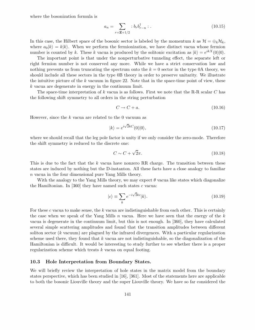
where the bosonization formula is
an =∑
r=Z+1/2
: brb†r−n : . (10.15)
In this case, the Hilbert space of the bosonic sector is labeled by the momentum k as H = ⊕kHk,where a0|k〉 = k|k〉. When we perform the fermionization, we have distinct vacua whose fermionnumber is counted by k. These k vacua is produced by the solitonic excitation as |k〉 = eikX(0)|0〉.
The important point is that under the nonperturbative tunneling effect, the separate left orright fermion number is not conserved any more. While we have a strict conservation law andnothing prevents us from truncating the spectrum onto the k = 0 sector in the type 0A theory, weshould include all these sectors in the type 0B theory in order to preserve unitarity. We illustratethe intuitive picture of the k vacuum in figure 22. Note that in the space-time point of view, thesek vacua are degenerate in energy in the continuum limit.
The space-time interpretation of k vacua is as follows. First we note that the R-R scalar C hasthe following shift symmetry to all orders in the string perturbation
C → C + a. (10.16)
However, since the k vacua are related to the 0 vacuum as
|k〉 = ei√
2kC(0)|0〉, (10.17)
where we should recall that the leg pole factor is unity if we only consider the zero-mode. Thereforethe shift symmetry is reduced to the discrete one:
C ∼ C +√
2π. (10.18)
This is due to the fact that the k vacua have nonzero RR charge. The transition between thesestates are induced by nothing but the D-instanton. All these facts have a close analogy to familiarn vacua in the four dimensional pure Yang Mills theory.
With the analogy to the Yang Mills theory, we may expect θ vacua like states which diagonalizethe Hamiltonian. In [360] they have named such states c vacua:
|c〉 ≡∑
k
e−i√
2kc|k〉. (10.19)
For these c vacua to make sense, the k vacua are indistinguishable from each other. This is certainlythe case when we speak of the Yang Mills n vacua. Here we have seen that the energy of the kvacua is degenerate in the continuum limit, but this is not enough. In [360], they have calculatedseveral simple scattering amplitudes and found that the transition amplitudes between differentsoliton sector (k vacuum) are plagued by the infrared divergences. With a particular regularizationscheme used there, they found that k vacua are not indistinguishable, so the diagonalization of theHamiltonian is difficult. It would be interesting to study further to see whether there is a properregularization scheme which treats k vacua on equal footing.
10.3 Hole Interpretation from Boundary States.
We will briefly review the interpretation of hole states in the matrix model from the boundarystates perspective, which has been studied in [16], [361]. Most of the statements here are applicableto both the bosonic Liouville theory and the super Liouville theory. We have so far considered the
141
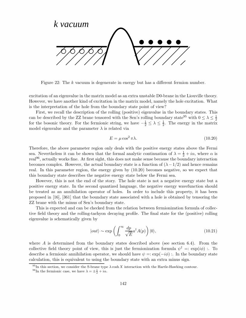
k vacuum
Figure 22: The k vacuum is degenerate in energy but has a different fermion number.
excitation of an eigenvalue in the matrix model as an extra unstable D0-brane in the Liouville theory.However, we have another kind of excitation in the matrix model, namely the hole excitation. Whatis the interpretation of the hole from the boundary state point of view?
First, we recall the description of the rolling (positive) eigenvalue in the boundary states. Thiscan be described by the ZZ brane tensored with the Sen’s rolling boundary state95 with 0 ≤ λ ≤ 1
2for the bosonic theory. For the fermionic string, we have −1
2 ≤ λ ≤ 12 . The energy in the matrix
model eigenvalue and the parameter λ is related via
E = µ cos2 πλ. (10.20)
Therefore, the above parameter region only deals with the positive energy states above the Fermisea. Nevertheless it can be shown that the formal analytic continuation of λ = 1
2 + iα, where α isreal96, actually works fine. At first sight, this does not make sense because the boundary interactionbecomes complex. However, the actual boundary state is a function of (λ−1/2) and hence remainsreal. In this parameter region, the energy given by (10.20) becomes negative, so we expect thatthis boundary state describes the negative energy state below the Fermi sea.
However, this is not the end of the story. The hole state is not a negative energy state but apositive energy state. In the second quantized language, the negative energy wavefunction shouldbe treated as an annihilation operator of holes. In order to include this property, it has beenproposed in [16], [361] that the boundary state associated with a hole is obtained by tensoring theZZ brane with the minus of Sen’s boundary state.
This is expected and can be checked from the relation between fermionization formula of collec-tive field theory and the rolling-tachyon decaying profile. The final state for the (positive) rollingeigenvalue is schematically given by
|out〉 ∼ exp
(∫ ∞
0
dp√Ea†A(p)
)|0〉, (10.21)
where A is determined from the boundary states described above (see section 6.4). From thecollective field theory point of view, this is just the fermionization formula ψ† =: exp(iφ) :. Todescribe a fermionic annihilation operator, we should have ψ =: exp(−iφ) :. In the boundary statecalculation, this is equivalent to using the boundary state with an extra minus sign.
95In this section, we consider the S-brane type λ coshX interaction with the Hartle-Hawking contour.96In the fermionic case, we have λ = ± 1
2+ iα.
142
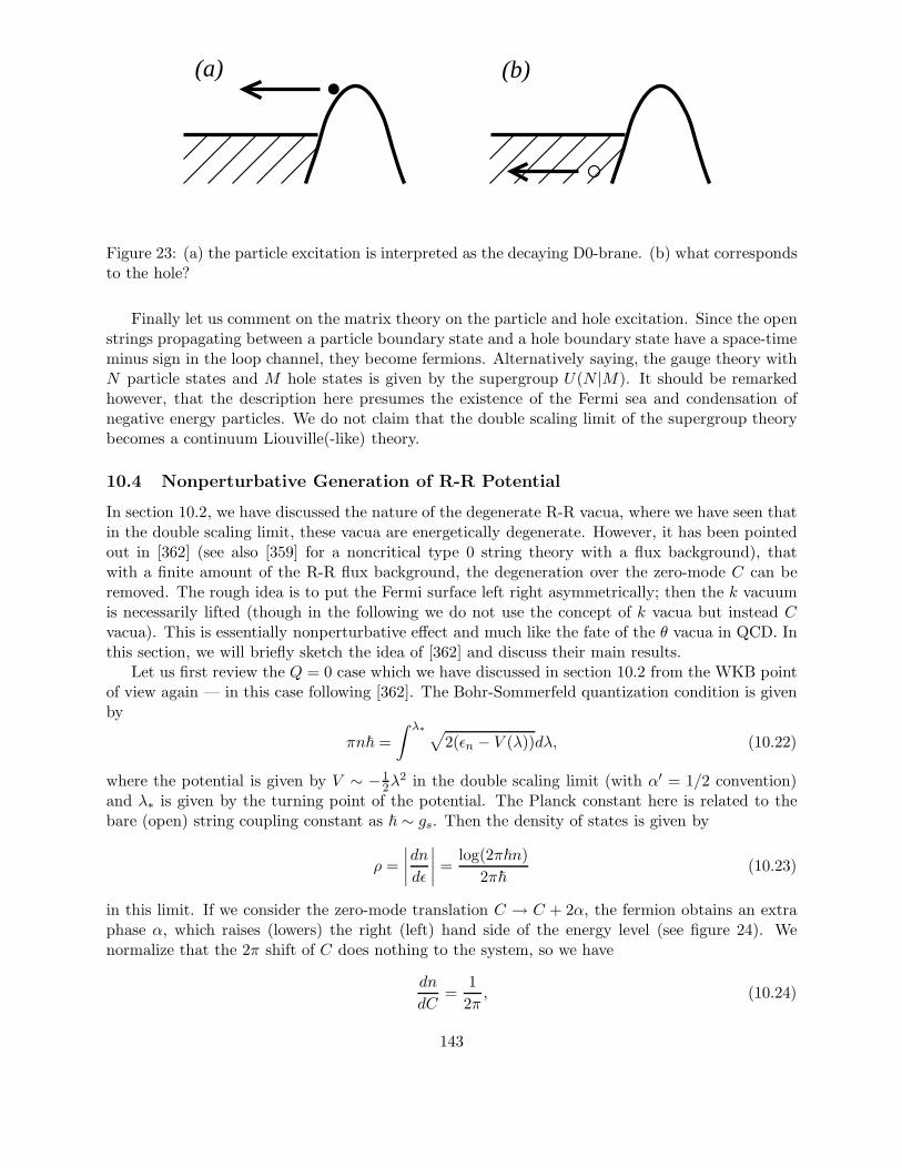
(a) (b)
Figure 23: (a) the particle excitation is interpreted as the decaying D0-brane. (b) what correspondsto the hole?
Finally let us comment on the matrix theory on the particle and hole excitation. Since the openstrings propagating between a particle boundary state and a hole boundary state have a space-timeminus sign in the loop channel, they become fermions. Alternatively saying, the gauge theory withN particle states and M hole states is given by the supergroup U(N |M). It should be remarkedhowever, that the description here presumes the existence of the Fermi sea and condensation ofnegative energy particles. We do not claim that the double scaling limit of the supergroup theorybecomes a continuum Liouville(-like) theory.
10.4 Nonperturbative Generation of R-R Potential
In section 10.2, we have discussed the nature of the degenerate R-R vacua, where we have seen thatin the double scaling limit, these vacua are energetically degenerate. However, it has been pointedout in [362] (see also [359] for a noncritical type 0 string theory with a flux background), thatwith a finite amount of the R-R flux background, the degeneration over the zero-mode C can beremoved. The rough idea is to put the Fermi surface left right asymmetrically; then the k vacuumis necessarily lifted (though in the following we do not use the concept of k vacua but instead Cvacua). This is essentially nonperturbative effect and much like the fate of the θ vacua in QCD. Inthis section, we will briefly sketch the idea of [362] and discuss their main results.
Let us first review the Q = 0 case which we have discussed in section 10.2 from the WKB pointof view again — in this case following [362]. The Bohr-Sommerfeld quantization condition is givenby
πn~ =
∫ λ∗√2(ǫn − V (λ))dλ, (10.22)
where the potential is given by V ∼ −12λ
2 in the double scaling limit (with α′ = 1/2 convention)and λ∗ is given by the turning point of the potential. The Planck constant here is related to thebare (open) string coupling constant as ~ ∼ gs. Then the density of states is given by
ρ =
∣∣∣∣dn
dǫ
∣∣∣∣ =log(2π~n)
2π~(10.23)
in this limit. If we consider the zero-mode translation C → C + 2α, the fermion obtains an extraphase α, which raises (lowers) the right (left) hand side of the energy level (see figure 24). Wenormalize that the 2π shift of C does nothing to the system, so we have
dn
dC=
1
2π, (10.24)
143

which shifts the energy bydǫL/R
dC= ± 1
2πρ, (10.25)
in the double scaling limit where ρ diverges as log ~. From this, when the original Fermi level inthe left and right potential is the same, the shift of C does not change the total energy, which iscompatible with what we have learned in section 10.2.
(a) (b)
Figure 24: Turning on the zero-mode of C corresponds to raising and lowering the left and righteigenvalues respectively.
Let us now fill the eigenvalues asymmetrically. Set µL = µ+Q and µR = µ−Q with a positiveQ < µ. Later, we will identify the parameter Q as the background flux of the theory.97 In thisbackground, the deformation by the shift of C changes the energy of the system, which is now givenby
V (C) =
∫ µL
µR
dǫρ(ǫR(C) − ǫR(0)) = −CQπ, (10.26)
in the double scaling limit. This is a perturbative result and requires a nonperturbative completion,for we should have a periodic potential because of the original identification C ∼ C + 2π. In otherwords, when C approaches π, the perturbed eigenvalues cross and the repulsion occurs as is alwaysthe case with the perturbation theory in the one dimensional quantum mechanics (see figure 25).
-2π-π -2π 2π2π -π0 π 0 π
Figure 25: When perturbed eigenvalues cross, the repulsion of eigenvalues occurs.
The identification of the Fermi level difference Q as the background flux can be understoodfrom the coupling of the flux to the world line tachyon, which is described by
S =
∫F(T ) ∧ F , (10.27)
97Note that the introduction of Q requires an infinite energy, and we should regard it as a different superselectionsector as opposed to the value of the infinitesimal deformation by the zero-mode C. This is much like the backgroundflux q in the type 0A theory. Indeed they are perturbatively related by the T-duality.
144
where F(T ) is in general an odd function of T and F is the dual field strength made from C [363].The contribution of this effect to the second quantized Hamiltonian for the fermion becomes
δH =
∫dλQΨ†(λ)Ψ(−λ), (10.28)
which directly implies that the (anti)symmetric part of Ψ has a Fermi level µ± = µ ± Q. Thesymmetric/antisymmetric classification used here is more suitable than the left/right classificationin the nonperturbative definition because of the tunneling effect. Also, it shows the stability ofthe nonzero Q background though energetically unfavored. It can be also seen from the fact thatthe T-dual of this configuration is the type 0A theory which has an imaginary R-R flux, where adifferent (real) R-R flux means a different nonperturbatively stable background.
In the following, we derive the full shape of the potential from the matrix model consideration.The Schrodinger equation for the eigenvalue in the double scaling limit can be written as
(d2
dx2+x2
4− a
)ψ(a, x) = 0, (10.29)
where λ =√
~
2x and ǫ = 12−~a. The Fermi level mismatch can be emulated by setting the system in
a box whose range is between xL/R = ∓√
2~+√
~
2C. Using the explicit solutions of the Schrodinger
equation, we can find that the energy a± which corresponds to the even/odd mode respectively isgiven by
φ0(a±) = ∓1
2arccos
[cosC√
1 + e−2πa±
]+ nπ, (10.30)
for each integer n, where φ0(a) = 12~
− 2a log√
2/~ + π2 + arg Γ(1
2 + ia). From this result, we canobtain the energy difference which depends only on C in the double scaling limit (other parts aredivergent as log ~ in this limit).
V (C) =1
2π
∫ µ+Q
µ−Qda arccos
[cosC√
1 + e−2πa
], (10.31)
which shows a correct periodicity and weak coupling limit µ→ ∞.Some comments are in order.
• At first sight, C is very massive with V ′′ ∼ eπµ. But as it is emphasized in [362], this does notmean that the space-time field C is massive. This is because the potential here is obtainedafter integrating over the Liouville volume Vφ ∼ log µ, and hence the actual “mass” in thespace-time is zero.
• We can do the same calculation with the compactified Euclidean time (finite temperaturematrix mode). The perturbative calculation shows the T-duality to the type 0A matrix modelwith an imaginary flux. Imaginary here should be related to the Wick rotation.98 However,it has been pointed out in [362] that the nonperturbative completion does not show the naiveT-duality. On the other hand, the “S-duality” which involves µ → −µ and C → C and aparticle/hole duality which exchanges NS and RR background are strict symmetries. See also[359], [364] for discussions on the T-duality. In the latter paper, the T-duality is studied fromthe duality between the double scaling matrix quantum mechanics and the instanton matrixmodel.
98We have encountered the imaginary flux also in the c = 0 model. See [334], [161].
145

• All those considered in this section are derived from the matrix model. It would be interestingto see its connection with the super Liouville theory. The D-instanton effects (with ZZ brane)must be one of the major sources.
10.5 Literature Guide for Section 10
While the study on the matrix model corresponding to the type 0 noncritical string theory hasa long history over a decade, its application to the type 0 theory has begun only recently [161],[351], [360], [16], [361], [330], [362], [67], [357], [353], [359], [358], [364]. However, we have alreadydiscovered many concrete (and exact) realizations of the nonperturbative string physics includingSen’s conjecture, the geometric transition, the nonperturbative generation of the R-R potential,various dualities which we have not met so far, and so on. We hope we will find more examples ofthese phenomena by investigating matrix models or the Liouville theory.
11 N = 2 Super Liouville Theory
In this section, we discuss the N = 2 supersymmetric Liouville theory. The N = 2 Liouville theoryis in a sense very different from the N = 0, 1 Liouville theory discussed so far. One of the majordisinctions is the nonrenormalization of the cosmological constant operator and the consequentdisappearances of the c(c) = 1 barrier. Because of this lack of the barrier, we can use the N = 2super Liouville theory as an “internal SCFT” in the general d > 2 superstring theory. In the nextsection, we use the N = 2 super Liouville theory as a building block of the superstring theorypropagating in the singular CY space. The organization of this section is as follows.
In section 11.1, we discuss the bulk theory. In subsection 11.1.1, we review the basic setup ofthe N = 2 super Liouville theory and its CFT properties. In subsection 11.1.2, we attempt toobtain the bulk structure constants but face a difficulty which we have not met in the N = 0, 1theory. The dual action proposal will be discussed to overcome this difficulty.
In section 11.2, branes in the N = 2 super Liouville theory are discussed. After reviewing thebasic modular transformation properties of the N = 2 characters in subsection 11.2.2, and 11.2.3,we construct the boundary states by using the modular bootstrap method.
In section 11.3, we review the matrix model proposal of the N = 2 super Liouville theory. Insubsection 11.3.1 and 11.3.2 we discuss the basic properties of the Marinari-Parisi model which isa supersymmetric matrix model and proposed to be the dual of the N = 2 super Liouville theory.In subsection 11.3.3, we discuss its connection with the world sheet N = 2 super Liouville theory.
11.1 Bulk Theory
11.1.1 Setup
The N = 2 supersymmetric Liouville theory [365] can be seen in two ways. The first one is thatwe regard it as the quantization of the N = 2 supergravity on the worldsheet (see e.g. [305],[366], [367]). The second one is that we simply regard it as a particular (irrational) CFT withan accidental N = 2 supersymmetry [368], [4], [369]. Though the first perspective seems naturalfrom the experience with the N = 0, 1 super Liouville theory we have discussed so far, we will takethe second point of view. That is because if we take the first standpoint, we have to gauge theN = 2 algebra, which leads to the so called (2, 2) (noncritical) string. While it is mathematicallyinteresting, the physical application of the (2, 2) string is less clear.99 Therefore, to utilize our
99However, see [370] for a relation to the topological LST which involves the N = 2 Liouville sector.
146
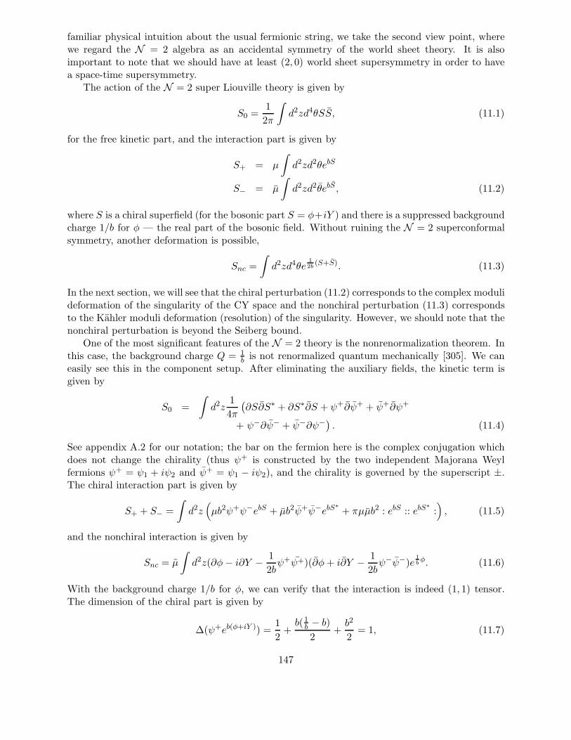
familiar physical intuition about the usual fermionic string, we take the second view point, wherewe regard the N = 2 algebra as an accidental symmetry of the world sheet theory. It is alsoimportant to note that we should have at least (2, 0) world sheet supersymmetry in order to havea space-time supersymmetry.
The action of the N = 2 super Liouville theory is given by
S0 =1
2π
∫d2zd4θSS, (11.1)
for the free kinetic part, and the interaction part is given by
S+ = µ
∫d2zd2θebS
S− = µ
∫d2zd2θebS , (11.2)
where S is a chiral superfield (for the bosonic part S = φ+iY ) and there is a suppressed backgroundcharge 1/b for φ — the real part of the bosonic field. Without ruining the N = 2 superconformalsymmetry, another deformation is possible,
Snc =
∫d2zd4θe
12b
(S+S). (11.3)
In the next section, we will see that the chiral perturbation (11.2) corresponds to the complex modulideformation of the singularity of the CY space and the nonchiral perturbation (11.3) correspondsto the Kahler moduli deformation (resolution) of the singularity. However, we should note that thenonchiral perturbation is beyond the Seiberg bound.
One of the most significant features of the N = 2 theory is the nonrenormalization theorem. Inthis case, the background charge Q = 1
b is not renormalized quantum mechanically [305]. We caneasily see this in the component setup. After eliminating the auxiliary fields, the kinetic term isgiven by
S0 =
∫d2z
1
4π
(∂S∂S∗ + ∂S∗∂S + ψ+∂ψ+ + ψ+∂ψ+
+ ψ−∂ψ− + ψ−∂ψ−) . (11.4)
See appendix A.2 for our notation; the bar on the fermion here is the complex conjugation whichdoes not change the chirality (thus ψ+ is constructed by the two independent Majorana Weylfermions ψ+ = ψ1 + iψ2 and ψ+ = ψ1 − iψ2), and the chirality is governed by the superscript ±.The chiral interaction part is given by
S+ + S− =
∫d2z
(µb2ψ+ψ−ebS + µb2ψ+ψ−ebS
∗+ πµµb2 : ebS :: ebS
∗:), (11.5)
and the nonchiral interaction is given by
Snc = µ
∫d2z(∂φ− i∂Y − 1
2bψ+ψ+)(∂φ+ i∂Y − 1
2bψ−ψ−)e
1bφ. (11.6)
With the background charge 1/b for φ, we can verify that the interaction is indeed (1, 1) tensor.The dimension of the chiral part is given by
∆(ψ+eb(φ+iY )) =1
2+b(1b − b)
2+b2
2= 1, (11.7)
147
and that of the nonchiral interaction, for example for the first term, is given by
∆(∂φe1bφ) = 1 +
1b (
1b − 1
b )
2= 1. (11.8)
Therefore, the background charge is not renormalized unlike in the bosonic or N = 1 Liouvilletheory. Because of this property, there is no analog of the c = 1 barrier in the N = 2 superLiouville theory. Note that the central charge of this theory is given by c = 3c = 3 + 3
b2and b can
be chosen as an arbitrary real number. Consequently, the central charge can become small enoughto introduce other transverse dimensions as opposed to the bosonic or N = 1 Liouville theory.Owing to this property, we can embed the N = 2 super Liouville theory into the superstring theorypropagating in the nontrivial background whose dimension is larger than two as we will see laterin section 12.2.
Let us show the explicit realization of the N = 2 world sheet superalgebra of this theory:
T = −1
2(∂Y )2 − 1
2(∂φ)2 +
1
2b∂2φ− 1
4(ψ+∂ψ+ − ∂ψ+ψ+)
G+ = −1
2ψ+(i∂Y + ∂φ) +
1
2b∂ψ+
G− = −1
2ψ+(i∂Y − ∂φ) − 1
2b∂ψ+
J =1
2ψ+ψ+ +
1
bi∂Y. (11.9)
The N = 2 mode algebra is given by
[Lm, G±r ] =
(m2
− r)G±m+r
[Lm, Jn] = −nJm+n
G+r , G
−s = 2Lr+s + (r − s)Jr+s +
c
3
(r2 − 1
4
)δr,−s
G±r , G
±s = 0
[Jn, G±r ] = ±G±
r+n
[Jm, Jn] =c
3mδm,−n, (11.10)
where the central charge is given by c = 3c = 3 + 3b2
. For the later purpose, it is convenient todefine the spectral flow generators as
U−1η LmUη = Lm + ηJm +
c
2η2δm,0
U−1η JmUη = Jm + cηδm,0
U−1η G±
r Uη = G±r±η. (11.11)
Anticipating the application to the superstring theory, we have a remark on the compactificationof the imaginary part of the superfield, Y . For the chiral interaction part of the action to be single-valued, Y should be compactified on the radius R = n
b with an integer n. Since the U(1) currentmeasures the momentum of Y , we have an integral U(1) charge for the NS sector if we have n = 1,the smallest radius. On the other hand, following the standard procedure, we can construct aspacetime supercharge operator from the N = 2 worldsheet superalgebra (see e.g. [368], [4]).
Qα =
∮dze−
σ2 e−
i2(H−QY )Sα, (11.12)
148

where H is the bosonized Liouville fermion and Sα is the flat space spinor operator. However,this supercharge operator becomes local only if the U(1) current has an integral spectrum in theunit 1/Q. Therefore, for the application to the spacetime superstring theory, the integral chargequantization of the NS sector is necessary. Of course, if we give up the spacetime SUSY (forexample, the type 0 string), this condition is not necessary.
Let us now go on to the primary states of the N = 2 Liouville theory [371], [372]. Thefundamental building block is given by the NS vertex operator
Nαα = eαS+αS∗= e(α+α)φ+i(α−α)Y , (11.13)
and the R vertex operator
R±αα = σ±eαS+αS∗
= σ±e(α+α)φ+i(α−α)Y , (11.14)
where σ± is the (left) spin operator and made up with the two dimensional left fermionic zero-modealgebra.100 The conformal dimensions of these operators are given by
∆N = −2αα+1
2b(α+ α)
∆R = −2αα+1
2b(α+ α) +
1
8(11.15)
and the U(1) charges are given by
wN =1
b(α− α)
w±R = w ± 1
2. (11.16)
It is important to note that if α = 0, we have 2∆N = wN , hence the chiral primary operator.Introducing the momentum P as
α+ α =1
2b+ iP, (11.17)
we can rewrite the conformal dimension as
∆N =P 2
2+
1
8b2+b2w2
2. (11.18)
As we can see from (11.16) (11.18), the U(1) charge and the conformal dimension does notchange if we reverse the momentum p → −p. As in the bosonic and N = 1 Liouville theory, weshould identify these operators up to a multiplicative constant, namely the reflection amplitude[372]. In the original exponential form, the identification map is given by
α → 1
2b− α
α → 1
2b− α. (11.19)
100For a complete vertex operator, we should tensor it with the right part properly according to the GSO projection.
149

11.1.2 Bulk structure constants and dual action
The fundamental goal in this subsection must be, of course, to derive various structure constantswhich characterize this SCFT. However, because of the technical difficulty which we will explainbelow, the derivation of the structure constant seems difficult without a further assumption. Themost difficult point is that we do not have a duality such as b→ b−1. This is because the backgroundcharge is not renormalized and b → b−1 changes the central charge as a result. This duality hasplayed a significant role in specifying the structure constant uniquely from the functional relations.Even in the N = 2 theory, we are actually able to derive a functional relation by using Teschner’strick, but we have only one relation, which is not enough to determine the structure constantuniquely.
To overcome the situation, a new kind of duality is proposed in [372] (see also [373], [374], [375]).The claim is that the N = 2 super Liouville theory perturbed by the chiral interaction S+ + S−with the cosmological constant µ is equivalent to the N = 2 super Liouville theory perturbed bythe nonchiral interaction Snc with the dual cosmological constant µ. Of course, we use the samebackground charge 1/b to ensure that the central charge remains the same. In section 12.3, wemake an attempt to give its proof after reviewing the necessary background, but we have someremarks here.
• In the neutral sector where the U(1) current J = 0, this conjecture seems to yield the correct(or at least consistent) bulk two-point function as we will see [373].
• From the viewpoint of the superstring propagating in the singular CY space [376], [377], [378],[379], [380], [381], the chiral deformation corresponds to the complex moduli deformation andthe nonchiral deformation corresponds to the Kahler moduli deformation. Therefore, if thesedeformations yield the same results, we should expect a mirror type duality. Perhaps, thisconjectured duality, if any, should involve the flipping of the GSO projection, or may be trueonly in the limited sector. Furthermore, if we restrict ourselves to the strings propagatingin the singular ALE space, the deformation of the singularity by the complex deformationand the Kahler deformation is actually the same thing (see appendix B.6 for a discussion).Therefore we expect the deformation by the real cosmological constant µ is related to thenonchiral deformation of the Kahler potential.101
In the following, we assume this duality and obtain the reflection amplitude by using Teschner’strick. Concentrating on the neutral sector α = α, we have basic degenerate operators
N− b2
= e−bφ
R±− 1
4b
= σ±e−12bφ. (11.20)
The OPE of any NS field with the degenerate operator N− b2
is given by
NαN−b/2 = Nα−b/2 + CN− (α)Nα+b/2, (11.21)
where the fusion coefficient CN− can be calculated by the usual perturbation saturation assumptionas
CN− = µµ〈e( 1b−2α−b)φ(∞)e2αφ(1)e−bφ(0)
101However, it is not clear whether we can deform the theory by the complex (θ term like) Kahler parameter withoutviolating the superconformal properties.
150

∫d2z2d
2z1ψ+(z1)ψ
−(z1)eb(φ+iY )(z1)ψ
+(z2)ψ−(z2)e
b(φ−iY )(z2)〉free. (11.22)
Performing the free field path integral and integration over z1, z2 (the Dotsenko-Fateev formula(A.14) is useful to evaluate the integration), we have
CN− (α) = κ1γ(1 − 2αb)γ(1/2 − 2αb− b2)γ(−1/2 + 2αb)γ(2αb + b2), (11.23)
where κ1 is an α independent constant which is proportional to µµ. The two-point functions wewould like to determine can be written as
〈Nα(z)Nα(0)〉 =DN (α)
|z|4∆Nα
〈R+α (z)R−
α (0)〉 =DR(α)
|z|4∆Rα. (11.24)
If we consider an auxiliary three-point function 〈Nα+b/2NαN−b/2〉, we have the following func-tional relation:
CN− (α)DN (α+ b/2) = DN (α). (11.25)
Of course its solution is not unique. To obtain the dual functional relation, we need a dual actionassumption. Consider the following OPE
NαR+−1/4b = R+
α−1/4b + CN− (α)R+α+1/4b
R−αR
+−1/4b = Nα−1/4b + CR−(α)Nα+1/4b. (11.26)
The first order insertion of the dual action determines the structure constants as
CN− (α) = κ2γ(2α/b − 1/2b2)
γ(2α/b)
CR−(α) = κ2γ(2α/b − 1/2b2 + 1)
γ(2α/b + 1), (11.27)
where κ2 is proportional to the dual cosmological constant µ. If we consider auxiliary three-pointfunctions, 〈R−
α+1/4bNαR+−1/4b〉 and 〈Nα+1/4bR
−αR
+−1/4b〉, we have
CN− (α)DR(α+ 1/4b) = DN (α)
CR−(α)DN (α+ 1/4b) = DR(α). (11.28)
These are the second functional relations. Solving these, we obtain
DN (P ) = µ−2iP/bΓ(1 + iPb )Γ(1 + iP b)Γ(1
2 − iP b)
Γ(1 − iPb )Γ(1 − iP b)Γ(1
2 + iP b)
DR(P ) = µ−2iP/bΓ(1 + iPb )Γ(1 − iP b)Γ(1
2 + iP b)
Γ(1 − iPb )Γ(1 + iP b)Γ(1
2 − iP b), (11.29)
where µ is a renormalized cosmological constant which is proportional to µ, whose precise form canbe found in the original paper [372], and we have introduced the momentum P as in (11.17). Forthe later purpose, it is important to note that this can be rewritten as
DN (P ) = µ−2iP/b Γ( iPb )Γ(1 + 2iP b)Γ(12 − iP b)2
Γ(− iPb )Γ(1 − 2iP b)Γ(1
2 + iP b)2(11.30)
by using the Legendle duplication formula (A.37) up to an irrelevant sign.Some consistency checks of the results are done in the original paper [372]. We will see in the
next section that this reflection property is consistent with the one-point function on the disk.
151

11.2 Branes in N = 2 Super Liouville Theory
In this section, we derive the Cardy states for the branes in the N = 2 super Liouville theory. Theessential difficulty here is the lack of the b → b−1 duality, so Teschner’s trick does not determinethe one-point function uniquely. Nevertheless, we recall that in the bosonic and N = 1 Liouvilletheory, we have another approach which yields the same result without resorting to the dualityargument. This has been done by what is called the modular bootstrap method [382], [383].
The basic strategy of the modular bootstrap (see section 5.2.2, 8.2 and 8.3 for example) is thatwe first assume the open spectrums and then modular transform them into the closed exchangechannel to obtain the Cardy boundary states (the boundary wavefunctions, or equivalently thedisk one-point functions). The identity representation was modular transformed into the (1, 1) ZZbrane and the general nondegenerate representation was transformed into the FZZT brane in ourprevious case. Of course, this method does not guarantee that these candidate Cardy states reallysatisfy the Cardy condition. We have to check this in the end, but from the experience with thebosonic and N = 1 Liouville theory, we expect this is the case.
11.2.1 Modular transformation of N = 2 character
To utilize the modular bootstrap method to obtain the Cardy states, we need to know the modulartransformation properties of the basic N = 2 representations. In this section we review theirproperties [384], [385], [382]. For simplicity, we concentrate on the NS sector because the charactersof other spin structures can be obtained by the spectral flows. We denote the conformal dimensionand U(1) charge as h,Q and set q = e2πiτ , y = e2πiz .
The unitary representation102 of the N = 2 algebra is classified into the following three types.
1. massive representations :
chNS(h,Q; τ, z) = qh−(c−1)/8yQθ3(τ, z)
η(τ)3(11.31)
which is spanned by operating L−n,J−n,G±−r to the highest primary states which is not an-
nihilated by any of these. The unitarity demands h > |Q|/2, 0 ≤ |Q| < c − 1. In the closedsector, the general vertex operator eαS+αS∗
belongs to this representation.103
2. massless matter (chiral or anti-chiral) representations :
chNSM (Q; τ, z) = q|Q|2
−(c−1)/8yQθ3(τ, z)
(1 + ysgn(Q)q1/2)η(τ)3(11.32)
which is defined by G+−1/2|Q〉 = 0 or G−
−1/2|Q〉 = 0 for chiral and anti-chiral respectively. The
unitarity demands h = |Q|/2, 0 ≤ |Q| < c. In the closed sector, the general vertex operatoreαS belongs to this representation.
3. graviton (vacuum) representations :
chNSG (τ, z) = q−(c−1)/8 (1 − q)θ3(τ, z)
(1 + yq1/2)(1 + y−1q1/2)η(τ)3(11.33)
102To construct a physically meaningful theory, we here deal with the unitary representation exclusively. Note thatthis requirement excludes the branes such as general (m,n) 6= (1, 1) ZZ branes.
103The second unitarity condition seems to restrict the allowable U(1) charge, but actually it is not the case. Byusing the integral spectral flow (11.11), we obtain Q → Q + (c − 1)n, and this generates other U(1) charge sectors.Also in the chiral sector, we have only finite operators in the physical theory because of this bound. However, oncewe twist the theory, this bound is removed, so for instance the analysis in [244] is consistent with the unitarity.
152
which is defined by G±−1/2|1〉 = 0 and L−1|1〉 = 0. This corresponds to the unique identity
operator in the theory.
The more general representations are generated by the spectral flows (11.11). Under these flows,the characters transform as
chNS(n; τ, z) = qc2n2ycnchNS(τ, z + nτ), (11.34)
for an integer n.The modular transformation of these characters are given in [386], [382]. The easiest one is the
massive representation, where we can simply use the modular transformation formula in appendix
A.4. We label the massive representation as h = p2
2 + w2b2
2 + 18b2 as in (11.18). Then the modular
transformation is given by
chNS(p2
2+w2b2
2+
1
8b2, w;−1
τ,z
τ
)= eiπ
cz2
τ b
∫ ∞
−∞dw′
∫ ∞
−∞dp′
e−2πiww′b2 cos(2πpp′)chNS(p′2
2+w′2b2
2+
1
8b2, w′; τ, z
). (11.35)
On the other hand, the modular transformations of the massless matter and graviton charactersare quite nontrivial104 and given by (see [386], [382] for the details)
chNSM
(λ, n;−1
τ,z
τ
)= eiπ
cz2
τ
[b
2
∫ ∞
−∞dw′
∫ ∞
−∞dp′e−2πi(b2λ+n)w′
cosh(2πp′b(1 + 12b2
− λ)) + e2πib2w′
cosh(2πp′b(λ− 12b2
))
2| cosh π(p′b+ iw′b2)|2 chNS
(p′2
2+w′2b2
2+
1
8b2, w′; τ, z
)
+i∑
n′∈Z
∫ 1+ 12b2
12b2
dλ′e−2πib2(λ+n/b2)(λ′+n′/b2)−(λ−1/2b2)(λ′−1/2b2)chNSM(λ′, n′; τ, z
)],
(11.36)
where n ∈ Z specifies the integer spectral flow and λ is the U(1) charge.Similarly for the graviton representations, we have
chNSG
(n;−1
τ,z
τ
)= eiπ
cz2
τ
[b
2
∫ ∞
−∞dw′
∫ ∞
−∞dp′e−2πinw′
sinh(πp′/b) sinh(2πbp′)| cosh π(p′b+ iw′b2)|2 chNS
(p′2
2+w′2b2
2+
1
8b2, w′; τ, z
)
+2∑
n′∈Z
∫ 1+ 12b2
12b2
dλ′ sin(π(λ′ − 1/2b2))e−2πin(λ′+n′/b2)chNSM(λ′, n′; τ, z
)]. (11.37)
104At first sight, one might try to expand the denominator as 1
1+yq1/2=∑∞
n=0(−1)n(yq1/2)n and modular transform
term by term (this can be done by the usual formula) and resum again. However, this does not yield the correctresults because the expanded characters contain infinitely heavy tachyon (imaginary momentum) contributions andthe modular transformation is ill-defined and divergent (see the similar argument in section 5.2.2). Indeed, the carefulevaluation of the modular transformation requires an additional massless matter sector contribution. One way to seeits necessity is to make a spectral flow and consider the R sector. The massless and graviton sector can possess anonzero Witten index, whereas on the other hand, if it were not for the contribution from the massless sector, theright-hand side would have a zero Witten index from the massive sector only.
153

However, this is not the end of the story. As has been stressed in [382], the right-hand side ofthe modular transformation above has a continuous U(1) charge spectrum and is not compatiblewith the local spacetime supercharge. Let us explain this point further. Suppose we compactifyY and hence we have a discrete U(1) charge in the closed sector (as we have stated in the lastsubsection, this is necessary to obtain the local spacetime supercharge operator). In this case, theIshibashi states made up with the closed states must have a discrete U(1) charge, but if we havesuch an open character as we have seen above, the U(1) charge in the closed exchange channelnecessarily contains a continuous U(1) charge, which is not what we want. It seems hopeless toobtain a discrete U(1) charge in the exchange channel by combining the open character by trialand error. Fortunately, for the rational central charge c = 1 + 2K
N with integers K and N , the“extended character” which preserves the discrete U(1) charge under the modular transformationhas been introduced in [382] (see also [387], [388]). The key idea is that we sum over the spectralflow.
The extended characters are defined as
χNS(h0, r, j0; τ, z) ≡∑
n∈r+NZ
qc2n2ycnchNS
(h0, Q =
j0N
; τ, z + nτ
)
χNSM (r, s; τ, z) ≡∑
n∈r+NZ
qc2n2ycnchNSM
(Q =
s
N; τ, z + nτ
)
χNSG (r; τ, z) ≡∑
n∈r+NZ
qc2n2ycnchNSG (τ, z + nτ) , (11.38)
where r, j0, s are the reference spectral flow parameters and U(1) charge and their ranges are
r ∈ ZN , 0 ≤ j0 ≤ 2K − 1, 1 ≤ s ≤ N + 2K − 1. (11.39)
Furthermore, we take j0 and s as integers in order to ensure the locality of the spectral flowgenerators. For the massive representations, we use the following convenient parameterization:
h ≡ h0 +rj0N
+Kr2
N=p2
2+j2 +K2
4NKj ≡ j0 + 2Kr, (11.40)
The modular transformations of the extended characters are given by
χNS(p, j;−1
τ,z
τ
)= eiπ
cz2
τ1√
2NK
∑
j′∈Z2NK
e−2πi jj′2NK
∫ ∞
−∞dp′ cos(2πpp′)χNS(p′, j′; τ, z), (11.41)
for the extended massive representations, and
χNSM
(r, s;−1
τ,z
τ
)= eiπ
cz2
τ
1
2√
2NK
∑
j′∈Z2NK
e−2πi (s+2Kr)j′2NK
∫ ∞
−∞dp′
cosh(2πbp′N+K−sN ) + ei
πj′K cosh(2πbp′ s−KN )
2| cosh π(p′b+ i j′
2K )|2χNS(p′, j′; τ, z)
+i
N
∑
r′∈ZN
N+K−1∑
s′=K+1
e−2πi(s+2Kr)(s′+2Kr′)−(s−K)(s′−K)
2NK χNSM (r′, s′; τ, z)
+i
2N
∑
r′∈ZN
e−2πi(s+2Kr)(2r′+1)
2N χNSM (r′,K; τ, z) − χNSM (r′, N +K; τ, z)
(11.42)
154
for the massless matter representations, and finally
χNSG
(r;−1
τ,z
τ
)= eiπ
cz2
τ
1
2√
2NK
∑
j′∈Z2NK
e−2πi rj′N
∫ ∞
−∞dp′
sinh(πp′/b) sinh(2πp′b)
| cosh π(p′b+ i j′
2K )|2χNS(p′, j′; τ, z)
+2
N
∑
r′∈ZN
N+K−1∑
s′=K+1
sin
(π(s′ −K)
N
)e−2πi r(s′+2Kr′)
N χNSM (r′, s′; τ, z)
(11.43)
for the graviton representations. Using these modular transformation properties, we will derive thedisk one-point functions in the following subsections.
11.2.2 Boundary conditions and Ishibashi states
The N = 2 superconformal symmetry allows the following two types of boundary conditions [389];for the A-type, we have
(Jn − J−n)|B〉 = 0(G±
r − iηG∓−r)|B〉 = 0, (11.44)
with η is either +1 or −1. For the B-type, we have
(Jn + J−n)|B〉 = 0(G±
r − iηG±−r)|B〉 = 0. (11.45)
Both of them are compatible with the N = 1 superconformal symmetry which we would like togauge
(Ln − L−n)|B〉 = 0(Gr − iηG−r)|B〉 = 0, (11.46)
where G = G+ + G−. Roughly speaking, the U(1) condition states that the A type imposesthe “Dirichlet boundary condition” on the Y coordinate, and the B type imposes the “Neumannboundary condition” on the Y coordinate. The η dependence simply yields the spin structures andthey are almost trivial, so we ignore these factors in the following.105
The Ishibashi states of the extended character are defined as (for example, we take the A-typebrane, for the B type we should replace J0 + J0 with J0 − J0.)
〈p, j|e−πtcHceiπz(J0+J0)|p′, j′〉 = δ(p − p′)δ(2NK)j,j′ χ(p, j; itc, z)
〈r, s;M |e−πtcHceiπz(J0+J0)|r′, s′;M〉 = δ(N)r,r′ δs,s′χM (r, s; itc, z)
〈p, j|e−πtcHceiπz(J0+J0)|r, s;M〉 = 0, (11.47)
which are constructed from the primary states appearing in the right-hand side of the modulartransformation formulae (particularly, we have K+1 ≤ s ≤ K+N−1). Then the Cardy boundarystates should be expanded as
〈B, ξ| =
∫ ∞
−∞dp
∑
j∈Z2NK
Ψξ(p, j)〈p, j| +∑
r∈ZN
N+K−1∑
s=K+1
Cξ(r, s)〈r, s;M |. (11.48)
105Note that if the (type II) space-time supersymmetry is possible, we should have both η = ± sector with the same
wavefunction. In a sense, it is guaranteed by the spectral flow unlike in the N = 1 theory.
155
In the next subsection, we determine the wavefunctions Ψξ(p, j) and Cξ(r, s) via the modularbootstrap method. To relate the results to the Liouville boundary parameter, we need the suitableboundary action for the N = 2 Liouville theory. This is given in [390] and we just quote the result:
SB =
∫ ∞
−∞dx
[− i
8π(ψ+ψ− + ψ+ψ−) +
1
4a∂xa
−1
4ebS
∗/2(µBa+
µb2
2µBa
)(ψ+ + ψ−) − 1
4ebS/2
(µBa+
µb2
2µBa
)(ψ+ + ψ−)
− 1
b2
(µ2B +
µ2b4
4µ2B
)eb(S+S∗)/2
], (11.49)
where a and a are (complex) boundary fermion operators and we have assumed the B-type boundarycondition here. We should also note that this boundary action is not enough to yield the FZZTtype disk one-point function unlike in the bosonic or N = 1 Liouville theory due to the lack of theduality. However we could use this boundary action to relate the boundary parameter µB to theCardy states continuous parameter as we will see in the next subsection.
11.2.3 Cardy boundary states
Now it is time to obtain the Cardy boundary states for the N = 2 super Liouville theory. Themodular bootstrap assumption106 is given by
eπcz2
τc 〈B;O|e−πτcHceiπz(J0+J0)|B; ξ〉 = χξ(ito, z′)
eπcz2
τc 〈B;O|e−πτcHceiπz(J0+J0)|B;O〉 = χG(r = 0; ito, z′), (11.50)
where to = 1τc
and z′ = −itoz. By using the modular transformation properties in section 11.2.1,we have [382], [383]
ΨO(p, j) =b
2
(2
NK
)1/4 Γ(12 + j
2K − ipb)Γ(12 − j
2K − ipb)
Γ(−ip/b)Γ(1 − 2ipb)
CO(r, s) =
√2
N
√sin(
π(s −K)
N), (11.51)
which is determined up to a (possibly p dependent) phase factor and a complex conjugation. Thiscan be fixed by demanding the reflection property which states
ΨO(p, j) = R(p, j)ΨO(−p, j), (11.52)
where the reflection amplitude R(p, 0) is given in (11.30). For nonzero j, it is given by
R(p, j) = µ−2ip/b Γ( ipb )Γ(1 + 2ipb)Γ(12 − ipb+ j
2K )Γ(12 − ipb− j
2K )
Γ(− ipb )Γ(1 − 2ipb)Γ(1
2 + ipb+ j2K )Γ(1
2 + ipb− j2K )
, (11.53)
which was first derived in [375]. It also determines the overall phase to be µ−ipb−1
, where µ is therenormalized cosmological constant which is proportional to µ. This boundary state correspondsto the (1, 1) ZZ brane in the bosonic Liouville theory and plays a fundamental role to derive other
106Whether these branes obtained via the modular bootstrap satisfy the Cardy condition or not is a nontrivialproblem. In [382], various cylinder amplitudes are calculated and the positivity of the spectral density is confirmed(at least for the particular parameter region).
156

boundary states. In [382], three classes of boundary states are proposed: the class 1 correspondsto the graviton representations, the class 2 corresponds to the massive matter representations andthe class 3 corresponds to the massless matter representations.
We can easily derive the other boundary wavefunctions from the modular bootstrap (11.50) andthe actual form of the modular transformation found in subsection 11.2.1. For example, the trivialone is given by the class 1 general graviton representations |B; r〉 which is given by
Ψr(p, j) = e−2πirjΨO(p, j). (11.54)
The class 2 boundary wavefunction (for the continuum part) is given by
Ψ(p′, j′; p, j) = µ−ipb−1 1
2b
(2
NK
)1/4 Γ(ipb−1)Γ(1 + 2ipb)
Γ(12 + j
2K + ipb)Γ(12 − j
2K + ipb)e−2πi jj′
2NK cos(2πpp′),
(11.55)which satisfies the reflection property. The relation between the boundary cosmological constantµB and the boundary parameter p′ is given in [383] by comparing the pole structure with theperturbative calculation; for j′ = 0, we have
(µ2B +
µ2b4
4µ2B
)=
µb
32πcosh(2πp′b). (11.56)
We will discuss the application of these boundary states to the supersymmetric cycle of thesingular Calabi-Yau space in the next section, but for the moment in this subsection, we discussthe c = 5 theory (two dimensional noncritical string theory) either in type 0 or type II [382].
For the type 0 string, we can choose the world sheet fermion GSO projection:
J0 + J0 ∈ 2Z (11.57)
for the type 0A theory orJ0 − J0 ∈ 2Z (11.58)
for the type 0B theory. For the type 0B theory, we have R-R charged A-branes and non R-Rcharged B-branes. The A-branes have Dirichlet boundary condition on the Y direction107, so theclass 1 A-brane is the D0-instanton and class 2,3 A-brane is the D1-instanton. Schematically, wehave
|B±〉A = |B〉NS ± |B〉R, (11.59)
where + corresponds to the BPS(-like108) brane and − corresponds to the antibrane. These arestable in the sense that the tachyon is projected out by the open GSO projection.109 Of course, ifwe consider the D-D system, we have open “tachyon” (for the class 2, this is actually a masslesstachyon). We should note that we have both even and odd dimensional “stable” branes in this caseas we have seen in the c = 1, N = 1 super Liouville theory.
107We can (and should in the supersymmetric case) compactify the Y direction, and regard it as the Euclidean time[391]. The Wick rotation in this case is very subtle especially in the supersymmetric case.
108Since space-time SUSY is missing in the type 0 theory, the “BPS” here does not have any deeper meaning thanbranes without an open tachyon.
109Unlike in the N = 1 theory, the open GSO projection for the class 2,3 branes can be imposed properly. Theessential reason is the existence of the spectral flow. At first sight, since the wavefunction for the R sector is differentfrom the NS sector (for example, compare eq (4.12) and (4.15) in [383]), the proper GSO projection does not seem tobe imposed. However, if we actually calculate the density of states, the integration (summation) over the U(1) chargemakes them equal (up to a sign which is related to the more involved GSO projection involving the U(1) charge).The author would like to thank Y. Sugawara for teaching the author this point.
157
The B-branes have Neumann boundary condition on the Y direction, and in the type 0B theory,we cannot have R-R Ishibashi states for this boundary condition. Therefore, the class 1 stateswhich correspond to the D0-branes have a genuine tachyon in the spectrum and this should yieldthe matrix dual of the type 0B N = 2 super Liouville theory in the double scaling limit. As wewill see in the next section, for the minimum radius R = 2 (M = 1), the dual theory is proposedto be the symmetric version of the KKK matrix model [392] though we cannot see any reason whythe vortex sector should be included from this holographic perspective. For the type 0A theory,the “stable” and “unstable” branes are just reversed. We have stable (with R-R sector) branesfor B-branes (D0 and D1) and unstable (without R-R sector) branes for A-branes (D0 and D1instanton).
Finally we consider the type IIB case. If we impose the spacetime SUSY, we should have theminimum radius R = 2. The boundary states for the A-branes are BPS and their properties aresimilar to those of the type 0B theory (with fermion sector). However note that the BPS branesexist both for odd dimension and even dimension as opposed to the naive free field guess. The moreinteresting boundary states are the B-branes which are non-BPS. For the class 1 brane, which isthe D0-brane and supposed to play a matrix holographic dual role in the double scaling limit, wefind an open tachyon and an open massless fermion in the spectrum [393], [382]. As we will discussin the next section, this is just the spectrum of the Marinari-Parisi super matrix model expandedaround the nonsupersymmetric vacuum [393].
11.3 Matrix Model Dual
In this section, we discuss the matrix dual theory for the c = 5 two dimensional type II N = 2super Liouville theory.110 The matrix model proposal for the discretized superstring was proposedin [393] and we will first review its properties in section 11.3.1 and 11.3.2. Then we compare itwith the continuum string theory in section 11.3.3.
11.3.1 Marinari-Parisi model
We will review the basic facts about the Marinari-Parisi model [394]. In this subsection, we followthe argument given by Dabholkar [395] (see also [396]), who truncated the model onto the diagonalgauge singlet sector as we will see. From the holographic point of view, this truncation is naturalbecause it has been shown [393] that the gauged Marinari-Parisi model which is naturally obtainedfrom the one dimensional theory on the D0-branes just corresponds to the Dabholkar’s truncation.
Ungauged original Marinari-Parisi model has the following action
S = −N∫dtdθdθTr
[1
2DΦDΦ +W0(Φ)
], (11.60)
where Φ is an Hermitian matrix valued superfield
Φ = M + θΨ + Ψθ + θθF, (11.61)
and D = ∂θ + θ∂t, D = −∂θ − θ∂t are super covariant derivatives. The Hamiltonian is given by
H =1
2Tr
(P 2 +
∂W0(M)
∂M∗∂W0(M)
∂M
)+∑
ijkl
[Ψ∗ji,Ψkl]
∂2W0(M)
∂M∗ij∂Mkl
, (11.62)
110We have called the two dimensional noncritical string “c = 1” and “c = 1” referring to the central charge of thematter section, but for the N = 2 super Liouville theory, the two dimension means no other matter sector. Thisleads to a somewhat different naming “c = 5” theory referring to the central charge of the Liouville part.
158

and the supercharges are given by
Q =∑
ij
Ψ∗ij
(P ∗ij − i
∂W0(M)
∂M∗ij
),
Q† =∑
ij
Ψij
(Pij + i
∂W0(M)
∂Mij
). (11.63)
The truncation done by Dabholkar is as follows. We diagonalize Φ by a unitary matrix. In general,this does not diagonalize Ψ and F simultaneously (see [397] for a related discussion). Nevertheless,we treat them as if they were diagonalized,
(UΦU †)ii = λi + θψi + ψ†i θ + θθfi. (11.64)
This truncated theory turns out to be a consistent subspace of the whole theory and makes a propersense. The reduced Hilbert space is spanned by the following states:
f(λ)∏
k
ψ†mk
|0〉. (11.65)
On these states, the supercharges act as
Q =∑
i
ψ†i
(−i ∂∂λi
− i∂W0
∂λi
)
Q =∑
i
ψi
−i ∂∂λi
+ i∂W0
∂λi− i∑
l 6=i
1
λi − λl
. (11.66)
At first sight, this expression for the supercharges seems peculiar and looks inconsistent becauseQ is not Hermitian conjugate of Q in a naive sense. However, this is because the innerproduct weshould use is a nonstandard one due to the Jacobian from the change of variables. It is convenientto use a standard innerproduct by rescaling the wavefunction as φ → J1/2φ and operators asO → J1/2OJ−1/2. With these rescaling we finally have
Q =∑
i
ψ†i
(−i ∂∂λi
− i∂W
∂λi
)
Q =∑
i
ψi
(−i ∂∂λi
+ i∂W
∂λi
), (11.67)
with an effective superpotential W which is given by
W = W0 −∑
i<j
log(λi − λj). (11.68)
11.3.2 Double scaling limit and collective field theory
In the last subsection, we have introduced the Marinari-Parisi supermatrix model. Here we attemptto take the double scaling limit and obtain the (super)string theory if any. The alternative approachto obtain the string theory is to use the collective field theory method as we have discussed in section3.2.2. The most difficult point here for the both methods is that the manifestly supersymmetrictreatment demands that the Fermi level µ is not an independent parameter and the flight of time
159
is finite so the Liouville like extra dimension seems to be compact. In contrast, as we will seein the next subsection, the continuum R-NS type construction of the two dimensional superstringdemands that the Euclidean time is compact and the Liouville direction is noncompact. We willnot solve this discrepancy here, but just review the facts so far obtained in the literature.
The double scaling limit of the Marinari-Parisi model in the singlet sector has been studied in[394], [395]. If we take the special choice of the cubic superpotential: W0 = 1
2Tr(gΦ − 13Φ3), the
bosonic effective potential can be written as
V (λ) =1
2
(λ+
1
4(λ2 − g)2
). (11.69)
The double scaling limit can be obtained by the scaling ansatz:
λ = λc(1 + az), λc = 2−1/3,
g = gc(1 + a2z), gc = 3 · 2−2/3, (11.70)
and we make a → 0, N → ∞ keeping Na5/2 = κ fixed. Unlike in the bosonic case, we haveto rescale the Euclidean time further111 as t = −ia−1/2τ . Then the effective action for the topeigenvalue can be written as (see [395] for the details)
S[z] =1
κ
∫dτ
[1
2
(∂z
∂τ
)2
+1
2(v′(z))2 + κψ† ∂ψ
∂τ+ κψ†ψv′′(z)
], (11.71)
where the superpotential v(z) is given by
v(z) =1
5(3 − z)(z + 2)3/2. (11.72)
The bosonic potential becomes V = 18(z + 2)(z − 1)2 and looks like it is not positive definite, but
we have to supply the infinite wall at z = −2. We will not study its properties any further, but weshould remark that this effective action breaks supersymmetry by the nonperturbative quantumeffect [395]. Indeed, this can be easily seen from the original superpotential. In the supersymmetricquantum mechanics, the supersymmetric condition uniquely fixes (if any) the wavefunction of thesupersymmetric ground states [399, 400] as
ψ(z) = e−2W (z), (11.73)
but in our case, the highest power of z in W (z) is odd (apart from the log term which antisym-metrizes the wavefunction). Therefore this wavefunction is not normalizable and the ground statemust be lifted via the tunneling effects.
Now let us go on to the collective field description of the Marinari-Parisi model [396], [401, 402].We expect that the collective fields yield the spacetime fields of the double scaling limit theory aswe have seen in the bosonic matrix model where the collective field describing the fluctuation ofthe Fermi surface becomes the spacetime tachyon field up to the nonlocal field redefinition. Theansatz here is
∂xϕ(x, t) =∑
i
δ(x − λi)
111This rescaling also has been under debate [398]. In any case, the rescaling makes sense only when t is noncompact.However, the naive holographic dual matrix model suggests that the Euclidean time variable should be compact inorder to preserve the space-time SUSY.
160
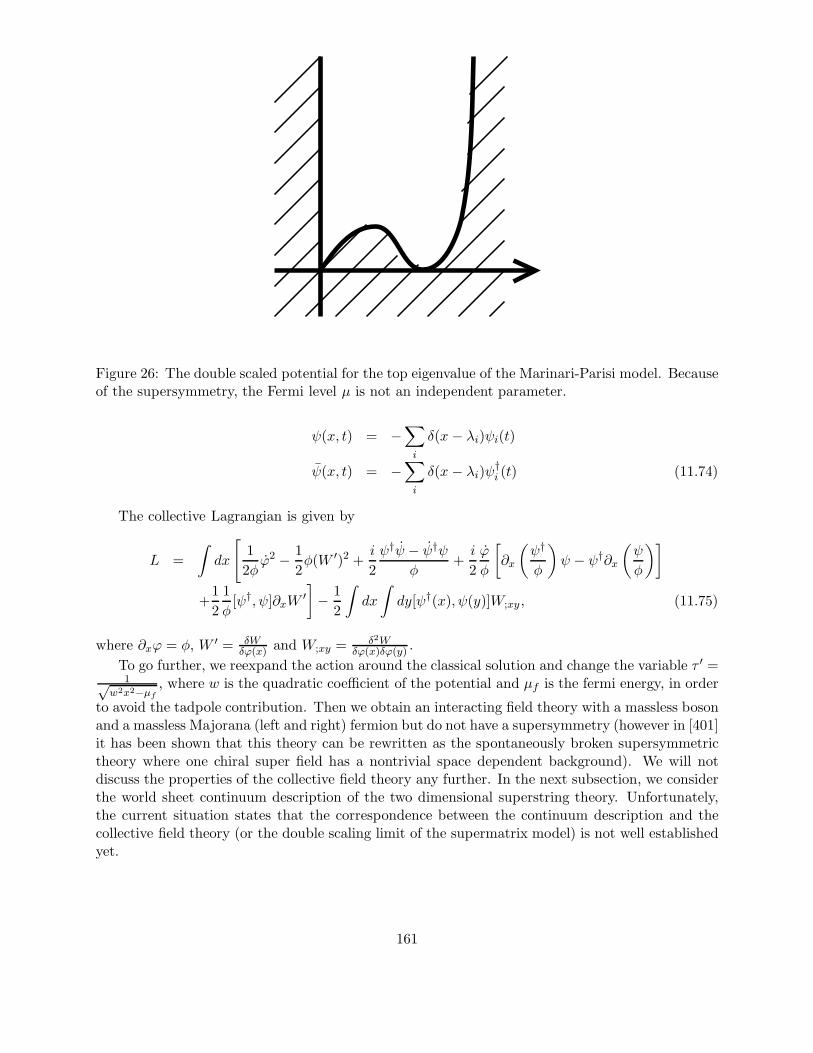
Figure 26: The double scaled potential for the top eigenvalue of the Marinari-Parisi model. Becauseof the supersymmetry, the Fermi level µ is not an independent parameter.
ψ(x, t) = −∑
i
δ(x− λi)ψi(t)
ψ(x, t) = −∑
i
δ(x− λi)ψ†i (t) (11.74)
The collective Lagrangian is given by
L =
∫dx
[1
2φϕ2 − 1
2φ(W ′)2 +
i
2
ψ†ψ − ψ†ψφ
+i
2
ϕ
φ
[∂x
(ψ†
φ
)ψ − ψ†∂x
(ψ
φ
)]
+1
2
1
φ[ψ†, ψ]∂xW
′]− 1
2
∫dx
∫dy[ψ†(x), ψ(y)]W;xy , (11.75)
where ∂xϕ = φ, W ′ = δWδϕ(x) and W;xy = δ2W
δϕ(x)δϕ(y) .
To go further, we reexpand the action around the classical solution and change the variable τ ′ =1√
w2x2−µf, where w is the quadratic coefficient of the potential and µf is the fermi energy, in order
to avoid the tadpole contribution. Then we obtain an interacting field theory with a massless bosonand a massless Majorana (left and right) fermion but do not have a supersymmetry (however in [401]it has been shown that this theory can be rewritten as the spontaneously broken supersymmetrictheory where one chiral super field has a nontrivial space dependent background). We will notdiscuss the properties of the collective field theory any further. In the next subsection, we considerthe world sheet continuum description of the two dimensional superstring theory. Unfortunately,the current situation states that the correspondence between the continuum description and thecollective field theory (or the double scaling limit of the supermatrix model) is not well establishedyet.
161
11.3.3 Connection with the world sheet superstring theory
The Marinari-Parisi model has unusual properties as a two dimensional superstring theory. Itwould be interesting to see the connection with the continuum description of the two dimensionalsuperstring. We first construct the two dimensional superstring from the R-NS formulation byusing the N = 2 super Liouville theory technique which we have reviewed in the last section.
Let us first consider the spectrum of the two dimensional superstring theory [368], [4]. To dothis it is convenient to use the free field description of the N = 2, c = 5 super Liouville theoryand impose the chiral GSO projection. We first bosonize the fermionic partner of φ: ψ and thefermionic partner of Y : ψY as
ψ =1√2(eih + e−ih), ψY =
1√2(ieih − ie−ih), (11.76)
where h is a canonically normalized bosonic field (h(z)h(0) ∼ − log z). Then the vertex operatorfor the tachyon (in the (−1,−1) picture) is
Tk = exp[−(σ + σ) + ikY + αφ], (11.77)
where σ is the usual bosonized superconformal ghost βγ = ∂σ, and −α+ 1 = |k|. The (left part ofthe) R vertex is given by
V− 12
= exp
[−1
2σ +
i
2ǫh+ ikY + αφ
], (11.78)
in the −12 picture. To perform the chiral GSO projection, we define the spacetime SUSY operator
S:
S(z) = exp
[−1
2σ +
i
2(h+ 2Y )
]. (11.79)
Note that the zero-mode charge Q =∮S(z) satisfies Q2 = 0 in the two dimension, so the spacetime
SUSY algebra is rather a BRST algebra [368], [4]. Therefore, the connection between the collectivefield of the Marinari-Parisi model is not clear because the matrix model SUSY algebra has the usualrelation Q2 = H. The GSO projection demands that every physical states should have a local OPEwith (11.79). This projects onto
• NS sector: k ∈ Z + 12 .
• R sector: ǫ = −1, k ∈ Z > 0, or ǫ = +1, 0 > k ∈ Z + 12 .
Combining the left and right part, we have for the type IIB theory one (massless) tachyon withhalf integer momentum, one left moving R-R scalar with integer momentum and one left movingcomplex fermion with half integer momentum.112 This is just the manifestation of the fact thatthe spacetime SUSY requires that Y should be compactified with the radius R = 2.
Since we have learned the contents of the unstable branes in section 11.2, we can conjecture thedual matrix theory by the holographic correspondence. The natural object here is the class 1 (ZZtype) B-brane, which can be interpreted as the D0-brane localized in the strong coupling region[382], [393]. The spectrum is given by the (genuine) tachyon and a massless (complex) fermion. On
112In [369], [393], the same theory has been studied in the dual SL(2,R)/U(1) coset construction which should bedual by the mirror symmetry discussed in section 12.1.
162

the other hand, if we expand the Marinari-Parisi model with the superpotential W0 = 12Φ2− 1
3λ2Φ3
around the nonsupersymmetric critical point, we have
S = −N∫dτTr
[1
2(DτM)2 + ΨDτΨ +
1
2λ2M2 − 1
16λ2
]. (11.80)
Comparing this with the spectrum obtained from the unstable class 1 B-brane, we can see thisis the same. It is worthwhile mentioning, however, that the Euclidean time for the B-brane iscompactified unlike the Marinari-Parisi model.113
Despite many subtleties, some other supporting arguments are given in [393]. They include,
• Symmetry consideration: there are a fermion number (−1)F and a Z2 R symmetry both inthe Marinari-Parisi model (for the odd superpotential, hence the broken supersymmetry) andthe worldsheet theory.
• Ground states and instantons: The (supersymmetric) perturbative vacua for the Marinari-Parisi model are classified by the fermion number. However, the instanton effect ruins thefermion number conservation and the actual vacuum is something like the θ vacuum whichis the summation over the different fermionic states and diagonalizes the Hamiltonian. Onthe other hand, since we have a BPS instanton in this theory (the class 1 BPS A-brane), weexpect the similar things happen in the two dimensional space-time theory.
Perhaps the conjecture here has a much weaker support than any other matrix model dualitiesin this review, and we should study further both the Marinari-Parisi model itself and the continuumtheory. Before closing this subsection, we have a few remarks:
• The biggest mystery is what the actual target space is. This is a difficult problem since thestring theory admits a T-duality if we compactify the theory, and we do have a compactified“time” direction Y in this case. Also, the matrix model collective field is related to the stringfield via the non-local field redefinition, which may cause the difficulty in understandingthe space-time SUSY in the dual theory. Concerning this point, we should note that theHamiltonian in the matrix model is a conserved quantity, but the “Hamiltonian” in the space-time theory from the N = 2 super Liouville cannot be conserved because of the nontrivialbackground in the Y direction.
• The space-time SUSY algebra is not the same in the matrix model and in the world sheetcontinuum theory. This has already been recognized in [395], and they have stated that thedual world sheet theory is rather a Green-Schwarz type superstring than the R-NS formulationconsidered so far. However the Green-Schwarz superstring in the two dimension also has asubtlety concerning the realization of the kappa symmetry. The hybrid formalism of the twodimensional superstring is given in [403], and it would be interesting to see the connection.Also [359] has proposed a matrix model dual of the type II superstring regularized by theR-R background in contrast to the N = 2 super Liouville background. Since the world sheetdescription of the R-R background is beyond the scope of this review, we do not discuss thisinteresting subject here.
• Finally, the existence of the nontrivial double scaling limit as a naive continuum limit (su-perspace τ, θ, θ sigma model coupled to the Liouville theory) has been questioned in [398].
113The author is not quite sure whether this fact is crucial or not. In [393], the Wick rotation is performed and theodd winding modes are discarded. Also, if we decompactify Y , the space-time SUSY from the world sheet perspectivebecomes obscure.
163

The world sheet theory is interacting and in the IR, all the coordinates become massive. Thesubtle point here is the rescaling of the time t in the double scaling limit taken in [395]. Itwould be fair to say what the continuum theory (R-NS noncritical superstring or a Green-Schwarz type superstring or something else) corresponds to the double scaling limit of theMarinari-Parisi model is an open problem yet.
11.4 Literature Guide for Section 11
The bulk N = 2 super Liouville theory has been studied in [365], [404], [305], [366], [367], [368],[4], [369], [371], [372]. Also we can find many references on the N = 2 super Liouville theory inconnection with the holographic dual of the little string theory or singular CY space as we will seein the next section.
The boundary states for the N = 2 super Liouville theory has been studied in [380], [393] andfurther developed in [382], [383].
The earlier studies on the Marinari-Parisi [394] model have been done in [405], [406], [395],[407], [408], [396], [409], [410], [411], [412], [413], [397], [401], [398], [402]. Based on the unstableD0-brane spectrum, the duality between the Marinari-Parisi model and the N = 2 super Liouvilletheory has been proposed in [393]. The superstring theory from the N = 2 super Liouville theoryhas been reviewed in [4], [369].
Theoretically speaking, the N = 4 extended super Liouville theory is possible [414], [415], [367](see also [416, 417] for related discussions). As far as the author knows, however, the application tothe physical string theory is still in its infancy and study on the subject such as structure constantsor brane contents etc is still limited.
12 Applications
In this section, we discuss applications of the N = 2 super Liouville theory. The organization ofthis section is as follows.
In section 12.1, we discuss the fermionic string on the 2D black hole. In subsection 12.1.1 wereview the basic properties of the string spectrum of the theory, and in subsection 12.1.2, we discussthe duality of the 2D fermionic black hole and the N = 2 super Liouville theory. In subsection12.1.3, the matrix model dual proposal for the 2D fermionic black hole is reviewed.
In section 12.2, we review the application of the N = 2 super Liouville theory to the (non)criticalstring propagating in the singular Calabi-Yau space. In subsection 12.2.1, we discuss the bulk theoryand in subsection 12.2.2, we discuss the branes present in the singular Calabi-Yau space from thebranes in the N = 2 super Liouville theory we have discussed in section 11.
In section 12.3, we provide an explanation of the duality in the N = 2 super Liouville theoryby using other dualities discussed in this section.
12.1 Fermionic String on 2D Black Hole
In this section, we discuss the relation between N = 2 super Liouville theory and the type 0 stringtheory propagating on the 2D black hole.
12.1.1 SL(2,R)/U(1) supercoset model
Since the bosonic string propagating on the 2D (Euclidean) black hole is described by the stringtheory on the SL(2,R)/U(1) coset theory quantum mechanically (see section 6.5), we naturally
164
expect that the fermionic string propagating on the 2D black hole is described by the SL(2,R)/U(1)Kazama-Suzuki supercoset theory [418]. In this section, we review its construction following [378,392].
Consider first the superconformal parent SL(2,R) theory at level k. This theory has the leftSL(2,R) super current
ψa + θ
√2
kJa, (12.1)
with a = 1, 2, 3, where
Ja = ja − i
2ǫabcψ
bψc. (12.2)
The free field OPE of ψa is given by
ψa(z)ψb(0) ∼ ηab
z(12.3)
where the metric is given by ηab = diag(+,+,−). The current ja satisfies the usual affine SL(2,R)algebra at level kB = k + 2. Then the total current satisfies
Ja(z)Jb(0) ∼k2η
ab
z2+iǫabcJ
c
z. (12.4)
The central charge of the theory is given by
c(SL(2,R)) =9
2+
6
k. (12.5)
It is convenient to define ψ± = 1√2(ψ1 ± iψ2) and bosonize them via
∂H = ψ2ψ1 = iψ−ψ+, (12.6)
with a canonically normalized bosonic field H; H(z)H(0) ∼ − log(z). Then J3 = j3 + i∂H.In order to make a quotient, we introduce two canonically normalized independent scalars X3
and XR. Our gauging condition is
J3 = −√k
2∂X3. (12.7)
XR is defined as
iH =
√2
kX3 + i
√c
3XR. (12.8)
where c = c(SL(2,R)/U(1)) = 3 + 6k . Let Φjm be the holomorphic part of the primary field in the
bosonic SL(2,R) theory. Its property is
j3(z)Φjm(0) ∼ mΦ(0)jmz
. (12.9)
Therefore
J3(z)Φjm(0) ∼ mΦ(0)jmz
. (12.10)
Using this operator, we can construct a primary of the bosonic quotient CFT on SL(2,R)/U(1):Vjm and that of the superconformal quotient: Ujm as
Vjmei 2m
k+2
√c3XRe
m√
2kX3 = Φjm
165
Ujmem√
2kX3 = Φjm. (12.11)
Furthermore we have the decomposition
einH = en(√
2kX3+i
√c3XR)
. (12.12)
Therefore, from a parent operator ΦjmeinH , we can construct a coset primary operator
V njm = Φjme
inHe−√
2k(m+n)X3 . (12.13)
Alternatively, we can eliminate the explicit X3 dependence and then we have
V njm = Vjme
i( 2mk+2
+n)√
c3XR . (12.14)
Their scaling dimensions are given by
∆(V njm) =
−j(j + 1) + (m+ n)2
k+n2
2. (12.15)
In the physical setup, we have k = 1/2 to obtain c = 15. The BRST invariant operator contentswith the GSO projection and their reflection property have been studied in [392].
12.1.2 2D fermionic black hole and N = 2 super Liouville duality
We have discussed the conjectural duality between the 2D black hole and the sine-Liouville theoryin section 6.5. Actually, the supersymmetric extension of this duality exists and its duality wasproved by using the mirror symmetry [419]. We would like to review the proof here. The gistis that we can find the gauged linear sigma model which flows to the SL(2,R)/U(1) supercosetmodel (which is the strict definition of what we call by the 2D fermionic black hole) in the IR, andwe dualize this action so that we obtain the dual action which flows to the N = 2 super Liouvilletheory in the IR. In this way we can prove the duality between the 2D fermionic black hole andthe N = 2 super Liouville theory (see also [378], [420]).
The relevant gauged linear sigma model action is
S =4
2π
∫d2zd4θ
[ΦeV Φ +
k
4(P + P + V )2 − 1
2e2|Σ|2
], (12.16)
where Φ and P are chiral superfields, V is a U(1) vector superfield and Σ is its field strength twistedchiral superfield.114 It has a gauge symmetry which transforms as follows:
Φ → ΦeiΛ
P → P + iΛV → V − iΛ + iΛ. (12.17)
The imaginary part of P is compactified, so P ∼ P + 2iπ. In the following, we present the roughsketch of the proof in the three steps. In the step-1 we show the IR equivalence of the gauged linearsigma model and the SL(2,R)/U(1) supercoset model. In the step-2 we dualize this gauged linear
114See appendix A.2 for our conventions of the superfield. 4 in front of the action is needed to connect our conventionswith those in [419].
166
sigma model. In the step-3 we show the IR equivalence of the dualized model and the N = 2 superLiouville theory.
Step-1: To show the IR equivalence of the gauged linear sigma model and the SL(2,R)/U(1)supercoset model, we first integrate out the massive field classically. The potential of the action(12.16) is given by
V = −D|φ|2 − |F |2 + |σ|2|φ|2 − k
2
(|Fp|2 − |σ|2 +D(p+ p)
)− 1
2e2D2. (12.18)
We integrate out σ and set D = F = Fp = 0. Then the D term condition is
D = |φ|2 + kRep = 0. (12.19)
Setting Imp = 0 by the gauge choice, we have a non-linear sigma model of φ as the effective action.The target space metric is
ds2 =
(1 +
r2
k
)dr2 +
r2
1 + r2
k
dθ2, (12.20)
where φ = r√2eiθ. However, this metric is not a 2D black hole metric. To see this, we set r =√
k sinh ρ then the metric becomes
ds2 = k(cosh4 ρdρ2 + tanh2 ρdθ2). (12.21)
Note this metric is not Ricci flat, so there must be non-trivial flow to obtain a conformal fix pointin the IR. Indeed there is such a correction and the one loop correction was studied in [419]. Wewill not reproduce the calculation here, but the result is that the perturbative correction changesthe metric (12.21) into that of the 2D black hole
ds2 = k(dρ2 + tanh2 ρdθ2) (12.22)
and it also generates the dilaton background so that the one-loop beta function vanishes.Actually we can show this IR flow even quantum mechanically. To show this, we use the similar
trick which is very common in the four dimensional superconformal gauge theory. First, we find theanomaly free R current in the UV theory which is assumed to be the superconformal R current inthe IR. Then we use the ’t Hooft anomaly matching argument [421] to calculate the central chargec of the IR theory. The anomaly matching states that this can be done in the UV theory which isfree.
In this case, the naive R current is anomalous, but we can improve it by adding the current of pwhich transforms anomalously because of the unusual gauge transformation (12.17). The improvedcurrent is (see the original paper [419] for a thorough derivation)
j+ = ψ+ψ+ +k
2χ+χ+ +
i
e2σ∂σ + i(Dzp−Dz p). (12.23)
The free OPE can be used to calculate the OPE of this current in the IR
j+(z)j+(0) = −1 + 2k
z2+ · · · . (12.24)
As a result we obtain the central charge of the IR theory:
c = 3
(1 +
2
k
), (12.25)
167
which coincides with that of the level k SL(2,R)/U(1) supercoset model.However, there is a subtly in the above reasoning. As is often the case, the anomaly free R
current is not unique. There is a freedom to add iaDz p to the above R current which makes thecentral charge c′ = 3 + 6(1 − a)/k. The question is what value of a corresponds to the actualsuperconformal current in the IR. In [419], it was shown that the mild assumption of the reality ofthe current uniquely chooses a = 0.115
To complete the proof, we have to show this IR theory which is superconformal and has acentral charge 3
(1 + 2
k
)and other parity symmetry is unique. In other words the question is
whether there is a marginal deformation which preserves all the symmetries of the SL(2,R)/U(1)super coset theory. After a thorough investigation, it can be shown this is the case unlike thebosonic SL(2,R)/U(1) coset.
Step-2: In this step, we dualize the action of the gauged linear sigma model. Here we treatthe action classically and in the third step we consider the quantum correction and the IR flow ofthe dualized action.
We would like to dualize the phase of Φ and the imaginary part of P . Concentrating on Φ forthe time being, let us consider the following action
S′ =4
2π
∫d2zd4θ
(eV+B − 1
2(Y + Y )B
), (12.26)
where B is a real superfield and Y is a twisted chiral superfield. If we integrate out Y first, thisenforces B to be decomposed as B = Ψ + Ψ, where Ψ is a chiral superfield. Substituting back thisinto the action, we obtain
S =4
2π
∫d2zd4θeV+Ψ+Ψ =
4
2π
∫d4θΦeV Φ, (12.27)
where we have introduced another chiral superfield Φ = eΨ. This is just the first part of the action(12.16). Alternatively we can integrate out B first, which gives
B = −V + logY + Y
2. (12.28)
Substituting back this into the action, we obtain the dual action
S =4
2π
∫d2zd4θ
(V
2(Y + Y ) − 1
2(Y + Y ) log(Y + Y )
)
=
∫4
2πd2zd4θ
[−1
2(Y + Y ) log(Y + Y )
]+
1
2
(4
2π
∫d2zdθ+dθ−ΣY + h.c.
). (12.29)
We can do the same dualization for P . We start with the following action
S′ =4
2π
∫d2zd4θ
(k
4(C + V )2 − 1
2(Yp + Yp)C
). (12.30)
115In the four dimensional case, it has been recently proposed that there is a procedure to find the correct conformalR current in the UV theory [422], [423], [424]. This is done by maximizing a which is supposed to be the fourdimensional analog of the monotony decreasing Zamolodchikov c function [425]. However, in this case this does notseem to apply (maximizing c does not make sense). Note that even the Zamolodchikov c theorem does not holdbecause c of the UV theory is 9, but that of the IR theory 3
(1 + 2
k
)can be arbitrarily large. This is because c does
not count the actual degrees of freedom of the theory with the linear dilaton coupling.
168

If we integrate out Yp then C = PY + PY as above so that we obtain the second part of the originalaction
S =4
2π
∫d2zd4θ
k
4(PY + PY + V )2. (12.31)
To dualize this action, we integrate out C instead, which yields PY + PY + V = 1k (Yp + Yp).
Substituting back this into the action,
S =4
2π
∫d2zd4θ
−1
4k(Yp + Yp)
2 +1
2
(4
2π
∫d2zdθ+dθ−ΣYp + h.c.
)
=4
2π
∫d2zd4θ
−1
2kYpYp +
1
2
(4
2π
∫d2zdθ+dθ−ΣYp + h.c.
)(12.32)
This is the dual action which we wanted. In the second line, we have used the fact that the F termof the chiral superfield is a total derivative.
Finally, collecting all the terms, we obtain the dual action
S =4
2π
∫d2z
∫d4θ
[− 1
2e2|Σ|2 − 1
2(Y + Y ) log(Y + Y ) − 1
2k|Yp|2
]
+1
2
(∫dθ+dθ−Σ(Y + Yp) + h.c.
)(12.33)
where Y and Yp have 2πi periodicity. Remember this action is derived classically since we haveneglected all the Jacobians of the transformation for the path integral measure and other quantumcorrections. The quantum corrections are discussed in the step-3.
Step-3: We consider here the quantum corrections of the dualization procedure and the IRflow of the effective action. We first note that the nonrenormalization theorem for the (2, 2) super-symmetry suggests that the twisted superpotential does not receive a perturbative correction butit may have a non-perturbative correction and the Kahler potential does receive perturbative andnon-perturbative corrections in general.
The origin of the nonperturbative correction for the twisted superpotential is instantons (orvortices in the two dimensions) as was discussed in [426] for the bosonic case. The usual super-symmetric holomorphy and symmetry argument shows this is the only correction. Therefore thetwisted superpotential from the instanton correction is
W = µe−Y , (12.34)
where µ is a dynamically generated scale. Note Yp does not have this kind of superpotential becauseit is not charged under U(1).
For a Kahler potential, one loop renormalization makes the metric
ds2 =|dy|2
2 log(Λ) + 2Rey+
1
k|dyp|2. (12.35)
Integrating out Σ gives a constraint Y + Yp = 0. Then we obtain the Kahler potential of Y
K(Y, Y ) = − 1
2k|Y |2 + · · · , (12.36)
where omitted terms are possible quantum corrections. The twisted superpotential of Y is now(because of the nonrenormalization theorem this does not suffer a quantum correction during theIR flow.)
W (Y ) = µe−Y . (12.37)
169
This is just the Liouville potential of Y ! If the Kahler potential is flat, then we have a (2,2)superconformal field theory with a central charge
c = 3
(1 +
2
k
). (12.38)
Actually even the flatness of the Kahler potential can be proven by deforming the UV theorywithout destroying any symmetry and using the uniqueness of the IR theory as discussed in thestep-1. An interested reader should consult the original paper [419].
To summarize the result, we obtain the dual action of the SL(2,R)/U(1) supercoset model:
S =4
2π
∫d2z
[∫d4θ
−1
2k|Y |2 +
1
2
(∫d2θµe−Y + h.c.
)], (12.39)
where Y has a period 2πi. This is the N = 2 super Liouville theory compactified on the r =√
2/kcircle. Its central charge is c = 3
(1 + 2
k
). Precisely speaking, we should redefine Y → −S. In
addition, Y is a twisted chiral superfield and not a chiral superfield. However, this does notmake any difference when we deal with only a twisted chiral field, for we can simply redefine thesupercoordinate θ− to θ−.
12.1.3 Matrix model for 2D fermionic black hole
The matrix model dual for the fermionic string propagating on the 2D black hole has been proposedin [392]. In the bosonic case, it is the r = 3/2 KKK matrix model which we have studied in section6.5.2. We recall that this conjecture has depended on the further duality between the bosonic 2Dblack hole theory and the sine-Liouville theory. In the fermionic case, we expect the duality (whichwe have provided the proof in the last subsection) between the 2D fermionic black hole and theN = 2 super Liouville theory plays an important role.
In the critical case, the dual super Liouville theory has the following super potential:
L = µ
∫d2θe
12(φ+iY ) + c.c = µ
∫d2θe
Q4
(φ+iY ) + c.c., (12.40)
where Q = 2, and the radius of Y is 2 (in the α′ = 2 unit). The conjecture made in [392] is that thedual matrix theory for the type 0B theory is the KKK matrix model at the selfdual radius R = 1(in the bosonic α′ = 1 unit) with a symmetric potential. The selfdual radius is selected becauseat this point, the sine-Liouville potential behaves (see 6.116) like e(φ+iX), which reminds us of thesuperpotential in the super Liouville theory. Therefore, we expect that the bosonic string theoryon the R = 1 sine-Liouville theory has similar correlators to those in the type 0B string on theN = 2 Liouville theory (up to leg factors and rescaling of momenta). The symmetric property ofthe potential is from the stability of the theory and the analogy to the duality between the N = 1type 0B super Liouville theory and the Hermitian matrix model with the symmetric potential.
Recalling that the N = 2 super Liouville theory is related to the fermionic black hole via duality,we have come to the following conjecture: the type 0A string theory on the SL(2,R) 1
2/U(1) black
hole is dual to the R = 1 KKK matrix model with a symmetric potential and eigenvalues fillingboth sides of the potential.
It would be interesting to study this conjecture further from many points of view. The scatteringamplitudes or partition function may be calculable.116 Also the study of the brane in this fermionic
116The calculation of the partition function from the matrix point of view seems a little bit difficult. This is becauseat R = 1, the method we have used in section 6.5.2 is not applicable.
170

string theory may yield the foundation of the conjecture as has been done in the 0A/B N = 1Liouville - matrix model duality. For the bosonic black hole geometry, we have briefly reviewed thepossible branes in the theory in section 6.5.3.
12.2 Strings and Branes in Singular Calabi-Yau Space
In this section, we discuss the application of the N = 2 super Liouville theory to the superstringspropagating in the singular Calabi-Yau space (times the flat Minkowski space). Unlike most of thepart in this review, we consider the D > 2 higher dimensional theory. This is possible because theN = 2 super Liouville theory admits a lower central charge owing to the nonrenormalization of thebackground charge.
12.2.1 Strings propagating in singular CY and N = 2 Liouville theory
We start this subsection by reviewing the world sheet description of the near horizon limit of theNS5-brane – Calan-Harvey-Strominger (CHS) background [427, 428][429] in the superstring theory.Remarkably, this geometry can be described by an exact solvable CFT.
First, we recall that the NS5-brane solution (for coincident branes) is given by
ds2 = e2φdx2 + dy2
e2φ(x) = C +N
x2
H = −Nǫ, (12.41)
where ǫ is the volume form of the unit-3sphere whose normalization is∫ǫ = 2π2 and integrally
quantized N is the number of NS5-branes, and C is the integration constant which determines theasymptotic string coupling. y is the tangential six dimensional coordinate and x is the transversefour dimensional coordinate. In the near horizon limit x→ 0, setting t =
√N log
√N/x2, we have
ds2 = dt2 +NdΩ23
φ = t/√N
H = −Nǫ, (12.42)
We can rephrase this geometry in the exact CFT language as follows. The internal CFT is
given by the super linear dilaton theory with the background charge Q =√
2N whose central
charge is cLD = 32 + 3Q2. On the other hand, the S3 part with H flux can be described by the
(supersymmetric) SU(2) WZW model with the level k = N − 2 whose central charge is cWZW =3kk+2 + 3
2 = 3(N−2)N + 3
2 . The total central charge becomes c = cWZW + cLD = 6, irrespective of thenumber of NS5-brane as it should be (we can also see that the tangential dimension is six). Thisinternal theory has (at least) an N = 2 superconformal algebra, so the six dimensional theory hasa space-time SUSY.
However, the string theory propagating in this CHS limit is actually singular. This is becausethe linear dilaton background forces us to have a strong coupling region as t → ∞ and nothingprevents strings from propagating in the strong coupling region. In other words, the Liouvilletheory in the µ→ 0 limit is singular as is easily seen from the identification gs ∼ µ−1.
The easiest way to regularize the situation is to turn on a Liouville potential. However, weshould be careful to preserve the space-time SUSY. For this purpose, the world sheet N = 2superconformal symmetry is necessary, and as a result the deformation by the N = 2 super Liouvillepotential becomes the best candidate. To do this, we have to supply compactified Y direction fromsomewhere, which is from the S3 part as we will explain in the following.
171

Before doing this, it is interesting to see the geometrical nature of turning on the N = 2 Liouvillepotential in this theory [378]. First of all, the N coincident NS5-branes are T-dual [376], [430] (seeappendix B.6 for a brief review) to the string theory propagating on the singular K3 whose complexstructure is given by
zN1 + z22 + z2
3 = 0. (12.43)
It has been proposed that turning on the Liouville potential corresponds to the deformation of thesingularity by the most relevant perturbation as
zN1 + z22 + z2
3 = µ. (12.44)
To go back to the NS5-brane picture, we rewrite (12.44) as
N∏
n=1
(z1 − r0e2πin
N ) + z22 + z2
3 = 0, (12.45)
where µ = (−r0)N . If we perform the T-duality, we have a system of N NS5-branes which aredistributed uniformly on a circle of radius r0.
NS5 ADE singularity
deformed singularity
T dual
T dual
Figure 27: The T-dual of NS5-branes is given by the ADE singularity. Turning on the Liouvillepotential corresponds to deforming the ADE singularity.
The general proposal [377], [378] for the near horizon limit of this system (for µ = 0) is thestring theory propagating on
Rd−1,1 × Rφ × S1 × LG(W = F ), (12.46)
where F = 0 is the defining equation of the (ADE type singular) CY manifold such as (12.44) andtechnically speaking, the GSO projection on the integer N = 2 U(1) charge sector is needed inthe super Liouville (Rφ and S1 part whose dilaton dependence is given by Q
2 φ) times the Landau-Ginzburg sector in order to ensure the space-time SUSY. This should be the dual theory of thedecoupling limit of the nongravitational string theory which propagates on the singular Calabi-Yauspace — what is called the little string theory (LST).
172
At first sight, this geometry is not related to the CHS background considered above, but as wewill see this is actually the same theory. The Landau-Ginzburg model with the super potentialW = zN1 + z2
2 + z23 corresponds to the N = 2 minimal model, which can be also constructed as
the coset SCFT SU(2)N
U(1) . The GSO projection acts as a ZN orbifold on SU(2)N
U(1) × S1, turning it into
SU(2)N . As a result, the target space (12.46) becomes R5,1 ×Rφ × SU(2), which is just the CHSbackground.
Now that we have a dual description (12.46) for the singular CY theory, it is easy to deformthis theory while preserving the N = 2 superconformal properties. Turning on the N = 2 superLiouville deformation:
δLc = µ
∫d2θe
1Q
(φ+iY ) + c.c. (12.47)
plays such a role. As we have stated earlier the nonchiral deformation:
δLnc = µ
∫d4θeQφ (12.48)
may be related to the Kahler deformation.We will not discuss an interesting physics of this bulk theory any further, but we have three
comments in order.
• This construction is closely related to the mirror duality of the N = 2 super Liouville theoryand the SL(2,R)/U(1) super coset model discussed in the last subsection. This is becausethe sigma-model whose target space is the non-compact deformed CY manifold F = µ isformerly described by the Landau-Ginzburg model with the superpotential
W = −µz−k0 + F, (12.49)
where k = 2Q2 . For the noninteger k, it has been proposed to interpret this theory as an
SL(2,R)/U(1) supercoset theory at level k. The proof of the duality between this theory andthe N = 2 super Liouville theory is the strong support of the dual description of the (doublescaling limit117 of the) LST.
• The original (µ = 0) LST is the decoupling limit of the non-gravitational theory on the coinci-dent NS5-branes. They have 16 space-time SUSY and do not have a dimensionless expansionparameter (for a review, see [431], [432]). The type IIA theory is a (2,0) supersymmetricconformal theory which has a tensor multiplet in the low energy limit which seems very mys-terious. On the other hand the type IIB theory is a (1,1) supersymmetric theory and has avector multiplet in the low energy limit and more familiar. The deformation considered abovecorresponds to higgsing the adjoint complex scalar as
〈Φ〉 = Cdiag(e2πiN , e
4πiN , · · · , e 2πiN
N ). (12.50)
The double scaling limit is the decoupling limit with fixed W-boson mass in this perspective[378].
117The double scaling limit here means µ → 0 and gs → 0 with x ≡ µ1
N gs fixed, which is just the KPZ scaling. Inthe singular limit, the physical amplitudes depend only on x as in the usual Liouville theory. The original definitionof LST corresponds to µ→ 0 and then gs → 0, hence x = 0.
173

• If we take the A-type singularity, we can replace the Landau-Ginzburg part with the N = 2minimal model of level k (c = k/(k + 2)). Then the criticality condition [382]
d
2+
k
k + 2+ (1 +
2K
N) = 5 (12.51)
leads to the conditiond = 6 : N = k + 2, K = 1, (12.52)
which is just the CHS background,
d = 4 : k = even, N = k + 2, K = (k + 4)/2k = odd, N = 2(k + 2), K = k + 4 (12.53)
which is related to the NS5-brane wrapped around the Riemann surface, and
d = 2 : N = k + 2, K = k + 3. (12.54)
which is related to the NS5-brane wrapped around the K3.
12.2.2 Branes wrapped around vanishing SUSY cycles
We have briefly reviewed the connection between the string theory propagating in the singularCalabi-Yau space in the double scaling limit and the N = 2 super Liouville theory in the lastsubsection. Now we have learned the bulk physics correspondence, it is good time to discuss therole of branes in the N = 2 super Liouville theory in the singular Calabi-Yau spaces [433], [434],[435], [380], [382]. In the following we focus on the A-type boundary condition which correspondsto the Dn-brane wrapped around the middle-dimensional SUSY cycles in CYn (special Lagrangiansubmanifold).
In our simple singular CY space, the special Lagrangian submanifold is easily obtained [436],[437], [380]. Let us parameterize the pair of roots of P (X) = Xk+2 +µ in the complex X plane as
Xa = (−µ)1/(k+2)eiπ(M+L)/(k+2),Xb = (−µ)1/(k+2)eiπ(M−L−2)/(k+2), (12.55)
where L = 0, 1, · · · ,[k2
], M ∈ Z2(k+2), and L + M ∈ 2Z. The vanishing Lagrangian submanifold
corresponds to the curve Cab connecting these pair of points, which is parameterized by (L,M).The BPS condition is given by
∫
Ca,b
|P (X)6−d
4 |dX = |∫
Ca,b
P (X)6−d4 dX|. (12.56)
which states that the phase of P (X)(6−d)/2dX is constant along the path Cab. It can be shown thatthe solution for the path Cab = γab is unique in our simple setting P (X) = Xk+2 +µ (for example,when d = 6 the solution γab is just the straight line). The Lagrangian submanifold is given by thefibration of sphere Sn−1 over γab whose radius vanishes at the end points Xa, Xb.
The brane wrapped around the Lagrangian submanifold is supersymmetric. Therefore, if we findthe (A-type) supersymmetric boundary states in the N = 2 super Liouville times super minimalmodel as we have seen in the last subsection, they should correspond to the vanishing cyclesconsidered above one to one. Since the description of the branes in the super Liouville theory hasbeen reviewed in section 11, the remaining ingredient needed here is the branes for the minimalmodel. Without going into the detail of the derivations, we just collect the relevant facts (see e.g.[438]).
174
The Cardy states for the minimal model are labeled by two integers L and M . For the NSsector, we should have L +M ∈ 2Z and for the R sector, we should have L+M ∈ 2Z + 1. Theyare made from the Ishibashi states by the Cardy’s formula.
The Liouville part brane has been discussed in the last section, but the relevant brane here isthe class 1 (ZZ type) brane which is localized in the φ→ ∞ strong coupling region. This is naturalsince the vanishing cycle is localized in the strong coupling region near the singularity of the CYspace.
Then the total boundary states is given by the closed sector GSO projected tensor product:√NPGSO (|L,M〉 ⊗ |B; r〉) , (12.57)
where PGSO projects onto the integral U(1) charge sector in order to ensure the space-time SUSY.We should note, however, that the PGSO does not necessary guarantee the open GSO projectionneeded for the supersymmetric cycle. Our remaining task is to impose this condition on the openspectrum and determine supersymmetric cycles.
Before doing this, we restrict our range of discrete parameters. First, since we find that param-eters M and r appear only through the combination M + 2r, we can simply set r = 0 (1/2) for NS(R) sector. Also if we consider only branes (no anti-branes) we can restrict ourselves to the rangeL = 0, 1, · · · ,
[k2
], because the minimal model branes have a property that the R part changes just
the sign when we perform the transformation L→ k−L and M →M + k+2 (for the NS part thischange does nothing, therefore this transformation exchange D-branes with anti D-branes).
To evaluate the overlap integral (cylinder amplitude) with the boundary states (12.57), we cansimply borrow the results in the last section and insert the GSO projection
δ(N)
(N
k + 2m+ β
)=
1
N
∑
r∈ZN
e−2πir( 1k+2
m+ 1Nβ), (12.58)
where β = j for the massive representations and β = s + 2Kr for the massless representations.The result is given by the summation over the character of the minimal model multiplied by thegraviton representations of the Liouville character:
eπcz2
τc 〈L1,M1|e−πτcHceiπz(J0+J0)|L2,M2〉
=
k∑
L=0
∑
r∈ZN
NLL1,L2
chL,M2−M1−2r(ito, z′)χG(r; ito, z
′), (12.59)
where NLL1,L2
is the fusion coefficients of SU(2)k and chL,M2−M1−2r(ito, z′) is the character for the
minimal model whose precise form can be found in [382] and we do not use it here. The importantpoint is that in order to ensure the open SUSY, we should have M1 ≡ M2 mod 2(k + 2). Thisparameter restriction is one to one corresponding to the vanishing cycle argument given in thebeginning of this subsection. Therefore we expect that the minimal model parameter L,M is justthe same parameter which specifies the vanishing cycle in (12.55).
As a further consistency check, the open Witten indices, which can be obtained by the spectralflow of the above results, have been calculated in [382]. These show desirable properties as inter-section numbers of the Lagrangian submanifold. For example, if we take L = 0 and d = 2, 6, wehave
I(0,M1|0,M2) = 2δ(2(k+2))(M1 −M2)− δ(2(k+2))(M1 −M2 − 2)− δ(2(k+2))(M1 −M2 + 2), (12.60)
which is the AN type extended Cartan matrix.
175

12.3 On the Duality of the N = 2 Super Liouville Theory
In section 11.1.2, we have discussed the conjectured duality [372] of the N = 2 super Liouvilletheory and its consequent result. This duality, if it holds, provides us a method to calculate variousstructure constants which we cannot determine from Teschner’s trick otherwise. The claim of theduality is that the N = 2 super Liouville theory with the perturbation:
S+ + S− =
∫d2zµb2ψ+ψ−ebS + µb2ψ+ψ−ebS
∗+ πµ2b2 : ebS :: ebS
∗: (12.61)
with a real µ is dual to the theory with the perturbation:
Snc = µ
∫d2z(∂φ− i∂Y − 1
2bψ+ψ+)(∂φ+ i∂Y − 1
2bψ−ψ−)e
1bφ, (12.62)
with the same b, hence the same central charge.In section 11.1.2, we have remarked that this duality is related to the hyper Kahler geometry
in the T-dualized NS5-brane perspective, where the complex moduli deformation and the Kahlermoduli deformation is related. Here we would like to prove the duality by combining other dualitieswhich we have learned so far.118 Note that this duality states that a certain Kahler potentialdeformation can be described by a superpotential deformation, which is interesting from the fieldtheoretical point of view (because we believe that the physics depending on the superpotential ismuch easier to handle than those depending on the Kahler potential). See also [260], [370] forrelated arguments.
Let us start from the N = 2 super Liouville theory with the smallest compactification radiusfor Y . From the mirror symmetry we have discussed in section 12.1.3, it is equivalent to theSL(2,R)/U(1) supercoset model (fermionic two dimensional black hole). Now we represent theSL(2,R)/U(1) supercoset model by the Wakimoto free field representation as we have done for thebosonic SL(2,R)/U(1) in section 6.5.1.
The supersymmetric Wakimoto representation is almost the same as that of the bosonic case ifwe recall the construction in section 12.1 (see [381] for a complete description). The bosonic partof the current is the same as that of the bosonic coset model except the level k becomes k + 2.We add three free fermions for the SL(2,R) fermionic partner and one more fermion for the U(1)current which is the super partner of X. Finally, we need a bosonic ghost for the super partner ofthe U(1) gauge fixed ghost. However, the fermionic part of the gauge fixing is almost trivial andthe net result is we have only two fermionic freedom. Since the U(1) BRST operator has becomethe same form as in the bosonic black hole, we have
QU(1) =
∮C(J3 + i
√k
2∂Y ) + fermionic term. (12.63)
Then we can eliminate the Wakimoto coordinates β,γ and ghost B,C (and their super partners)as has been done in the bosonic case (see 6.105). Since the bosonic part of the SL(2,R) currentand the U(1) BRST charge are the same, the actual result can be easily obtained by simplysupersymmetrizing the finial result of the bosonic theory. However, after eliminating the Wakimotocoordinates, the screening operator becomes nothing but the nonchiral deformation [380]:
Snc = µ
∫d2z(∂φ− i∂Y − 1
2bψ+ψ+)(∂φ+ i∂Y − 1
2bψ−ψ−)e
1bφ. (12.64)
118Technically speaking, we prove the duality only when Y is compactified on the smallest circle, which is preciselyrelated to the K3 geometry. It would be interesting to prove the duality with more general radii, which would providea more nontrivial duality in the NS5-brane or singular CY perspective.
176
This completes our proof of the conjectured duality of the N = 2 super Liouville theory. It wouldbe interesting to extend the result to the boundary theory and the more general radius case. Also itis a challenging problem to obtain the precise relation between the cosmological constant µ and thedual cosmological constant (black hole mass parameter) µ, which can be obtained from Teschner’strick argument as has been done in [372], along the same line of reasoning above. However, we findone difficulty; the mirror duality used here is essentially a nonperturbative effect and we have notbeen able to obtain the precise value for the dynamically generated scale so far.
12.4 Literature Guide for Section 12
Materials we have discussed in this section are closely related to each other via various dualities.The fermionic black hole has been discussed in [378, 392], but it is dual to the N = 2 super Liouvilletheory [419], [378], [260], [420]. Originally, this duality was conjectured from the dual little stringtheory which has been studied in [377], [378] in this context. This chain of duality and geometricalperspective leads us to the N = 2 duality conjectured in [372] as we have seen in section 12.3.As far as the author knows, the proof or explanation of the N = 2 duality is first presented inthis review, though the individual dualities have been known for years. See also [370] for relateddiscussions.
On the other hand, the exact description of the branes in the N = 2 super Liouville theory[382], [383] enables us to extend the earlier works [433], [434], [435], [380] and study the detailedphysics of the branes in the singular CY space. Since the space-time is higher dimensional, we donot expect that the matrix model-like description is possible, but even the world sheet analysis ofthe Liouville theory will reveal important physics of the NS5-brane and the singular CY space.
Part III
Unoriented Liouville Theory
13 Liouville Theory on Unoriented Surfaces
The bosonic Liouville theory on unoriented surfaces is discussed in this section. One of the moti-vations of this setup is to understand the properties of the orientifold plane under the nontrivialbackground. We use the α′ = 1 notation in this section. The organization of this section is asfollows.
In section 13.1, we derive the exact crosscap state in the Liouville theory from the modularbootstrap method and the conformal bootstrap method, and we discuss its properties.
In section 13.2, the tadpole cancellation in the c = 1 two dimensional unoriented string theoryis reviewed. In subsection 13.2.1, the free field calculation is presented and in subsection 13.2.2,the boundary-crosscap state calculation is presented. From both approaches we conclude that twoD1-branes are necessary to cancel the tadpole divergence. In subsection 13.2.3, on the other hand,alternative Fischler-Susskind mechanism is reviewed to deal with the crosscap tadpole.
In section 13.3, the matrix model dual of the unoriented Liouville theory is discussed. Insubsection 13.3.1, we discuss the unoriented c = 0 matrix model and compare some amplitudes withthe continuum Liouville calculation. In subsection 13.3.2, the unoriented c = 1 matrix quantummechanics is discussed and particularly the thermodynamic aspects of the unoriented c = 1 matrixmodel are investigated.
177

13.1 Crosscap State
The most fundamental object for the unoriented Liouville theory is the one-point function on theprojective plane. As in the one-point function on the disk, we can calculate it either by the directcalculation or by the crosscap state from the modular bootstrap. In this section, following [439], weobtain the projective plane one-point function first as a crosscap state from the modular bootstrapmethod and then check its consistency by the direct conformal bootstrap method.
Let us first review the building block of the crosscap state — the Ishibashi crosscap states [158].They satisfy the crosscap condition
(Ln − (−1)nL−n)|P,C〉 = 0. (13.1)
This equation is solved formally by
|P,C〉 =
(1 − L−1L−1
2∆P+ · · ·
)|P 〉 (13.2)
with any bulk primary state |P 〉. In the bosonic Liouville case considered here, we use e(Q+2iP )φ
as the (normalizable) primary states. The defining properties of the Ishibashi states are
〈P,C|e−πτc(Lc+Lc− c12
)|P ′, C〉 = δ(P − P ′)qP
2
η(iτc)
〈P,B|e−πτc(Lc+Lc− c12
)|P ′, C〉 = δ(P − P ′)qP
2
η(iτc + 12)
(13.3)
where q = e−2πτc is the closed modular parameter.With these Ishibashi states, we expand the Cardy crosscap state as
〈C| =
∫ ∞
−∞dPΨc(P )〈P,C| (13.4)
Our task is to determine the wavefunction Ψc(P ) which is proportional to the projective planeone-point function.
To do this, let us consider the Mobius strip amplitude bounded by the (1, 1) ZZ brane and thecrosscap state. This amplitude is highly constrained from the sewing constraint [440],[441], whichis the crosscap analogue of the Cardy condition. In the exchange channel, it becomes
ZM,(1,1)(τc) =
∫ ∞
−∞dPΨ(1,1)(−P )Ψc(P )
qP2
η(iτc + 12), (13.5)
where we can find the (1, 1) boundary wavefunction Ψ(1,1)(−P ) in (5.60). The open/closed dualityenables us to calculate the same amplitude in the open loop channel. Since the (1, 1) boundarystate contains only the identity operator, we expect that the same amplitude becomes in the openchannel,
ZM,(1,1)(τo) = Tro,(1,1)[Ωe−2πτo(Lo− c
24)] =
e−πτo2
(b+b−1)2 + e−πτo2
(b−b−1)2
η(iτo + 12 )
. (13.6)
In the more general case where the open spectrum is constructed by the (n,m) degenerate state,we have [439]
Tro,(n,m)[Ωe−2πτo(Lo− c
24)] =
e−πτo2
(nb+mb−1)2 − (−1)nme−πτo2
(nb−mb−1)2
η(iτo + 12)
. (13.7)
178
Note that the factor (−1)nm comes from the fact that the level nm null state has Ω = (−1)nm.In the Mobius strip case, the modular transformation is given by 1
4τc= τo. Using the modular
transformation formula in appendix (A.78), we can translate it into the closed exchange channel as
Tro,(1,1)[Ωe−2πτo(Lo− c
24)] =
∫ ∞
−∞dP
e−2πτcP 2
η(iτc + 12)
(cosh(π(b+ b−1)P ) + cosh(π(b− b−1)P )
). (13.8)
Comparing this with (13.6) and substituting the (1,1) boundary state wavefunction (5.60), we have
Ψc(P ) = (πµγ(b2))−iP b−1 21/4Γ(1 + 2iP b)Γ(1 + 2iP b−1)
2πiPcosh(πPb) cosh(πPb−1). (13.9)
To check its consistency, we use Teschner’s trick to derive the constraint on the crosscap one-point function and see whether this is satisfied or not. As we will see, the solution of the functionalrelation is not unique, but in any case we can check that the above wavefunction derived from themodular bootstrap is a consistent one.
First, let us review several basic facts about the correlation functions on the projective plane.The projective plane can be seen as a complex plane with the identification:
z ∼ −1
z. (13.10)
Therefore, the primary fields on one-point and on its image point are related as
φ(z, z) ∼ z−2∆z−2∆φ(−1/z,−1/z). (13.11)
This constrains (with SL(2,R) invariance) the form of the correlation functions as
〈φ(z, z)〉RP2 =c
(1 + zz)2∆(13.12)
and
〈φ(z1, z1)φ(z2, z2)〉RP2 =(1 + z2z2)
2∆1−2∆2
|1 + z1z2|4∆1F (η), (13.13)
where η is the crossratio:
η ≡ |z1 − z2|2(1 + z1z1)(1 + z2z2)
(13.14)
As in the disk case, we consider the auxiliary two-point function:
G(η) ∼ 〈Vα(z1, z1)V−b/2(z2, z2)〉RP2 , (13.15)
where the trivial conformal factor is omitted from the left-hand side. With the method of image,this amplitude is effectively given by
〈Vα(z1)V−b/2(z2)Vα(−1/z1)z−2∆α1 V−b/2(−1/z2)z
−2∆2,1
2 〉. (13.16)
Thus, evaluating this amplitude either by approaching z1 → z2 first or by approaching z1 → −1/z2first, and comparing their results, we obtain the functional relation for the one-point function:
〈Vα(z, z)〉RP2 =U(α)
|1 + zz|2∆α. (13.17)
179

z1 z2
=
z1 z2
-1/z2 -1/z1 -1/z2 -1/z1
Figure 28: We can calculate the two-point function on the RP2 by the method of image. Changingthe order of taking OPE enables us to obtain the two different expression for the two-point function.
The direct OPE as η → 0 yields
G(η) = C+U(α− b/2)F+(η) + C−U(α+ b/2)F−(η), (13.18)
where we have already calculated the OPE coefficient C± in section 5.1.1 (5.13)(5.14). The con-formal block F± is determined by the differential equation which the degenerate operator V−b/2should satisfy. These are given by119
F+(η) = ηbα(1 − η)bαF (2bα, 2bα − 2b2 − 1, 2bα − b2, η)
F−(η) = η1+b2−bα(1 − η)bαF (−b2, 1 + b2, 2 + b2 − 2bα, η) (13.19)
On the other hand, in the cross channel, we have
G(η) = C+U(α− b/2)F+(1 − η) + C−U(α+ b/2)F−(1 − η), (13.20)
where F±(1−η) is the same function as (13.19) with a different argument. From the hypergeometricfunction identity (A.46) and the actual form of C± we can write the functional relation for the one-point function U(α) as
U(α+ b/2) =Γ(2 − 2bα+ b2)Γ(−1 + 2bα− b2)
Γ(1 + b2)Γ(−b2) U(α+ b/2)
−γ(−b2)
πµ
Γ(2 − 2bα + b2)Γ(2bα − b2)
Γ(1 − 2bα)Γ(−1 + 2bα− 2b2)U(α− b/2),
U(α− b/2) =Γ(2bα − b2)Γ(1 − 2bα+ b2)
Γ(1 + b2)Γ(−b2) U(α− b/2)
− πµ
γ(−b2)Γ(1 − 2bα+ b2)Γ(−1 + 2bα− b2)
Γ(2bα)Γ(2 − 2bα+ 2b2)U(α+ b/2). (13.21)
Actually, the first equation is not independent of the second one as we can see they give the sameconstraint from a simple algebra. We can solve these constraints with the duality assumption
119Note that these functions are different from (5.17). This is because from our definition of the projective planecrossratio η, the operator identification with the four-point bulk operator is different from that has been done in thedisk case. In terms of the differential equation (4.27), we identify φ4 = Vα, φ3 = V−b/2 and φ1 = Vα here, but in thedisk case, we have had φ3 = Vα, φ4 = V−b/2 and φ1 = Vα.
180

b→ b−1 as,
U(α) =2
b(πµγ(b2))(Q−2α)/2bΓ(2bα − b2)Γ
(2α
b− 1
b2− 1
)f(α), (13.22)
where f(α) is given by the linear combination of
cos((b+ b−1)π(α−Q/2)), cos((b− b−1)π(α −Q/2)). (13.23)
Of course, we have already known that the actual combination is given by (13.9), but we will usethis constraint in the following to address some peculiar issues.
Using this crosscap state, we can calculate other Mobius strip amplitudes and Klein bottleamplitude. In the next section, we discuss their divergences and the possibility of the tadpolecancellation. For the time being, we ignore the divergences and consider their general properties.
First, we can calculate the (m,n) Mobius strip amplitude which is given by
ZMm,n =
∫ ∞
−∞dPΨm,n(P )ΨC(−P )
qP2
η(iτc + 12)
= 2
∫ ∞
−∞dP
qP2
η(iτc + 12)
sinh(2πmPb−1) sinh(2πnPb) cosh(πPb−1) cosh(πbP )
sinh(2πPb−1) sinh(2πbP ).(13.24)
With the trigonometric function formula:
sinh(2πnbP ) cosh(πbP )
sinh(2πbP )=
n−1∑
l=0
cosh(πbP (2l + 1)), (13.25)
we have [439]
ZMm,n(τc) =
m−1∑
k=0
n−1∑
l=0
Tro(2k+1,2l+1)[Ωe−2πτo(Lo− c
24)]. (13.26)
This is expected because this Mobius strip amplitude should yield the Ω projection of the cylinderamplitude (5.68) which is bounded both by the (m,n) boundary state.
Things are all consistent so far. However, when we consider the Mobius strip amplitude with theFZZT brane or the Klein bottle amplitude, situation becomes subtler. For example, we find thatthe Mobius strip partition function with the FZZT brane whose boundary parameter is s becomes
ZMs =
∫ ∞
−∞dP
qP2
η(iτc + 12)
Ψs(P )ΨC(−P )
=
∫ ∞
−∞dP ′ q(P
′)2
η(iτo + 12)ρs(P
′), (13.27)
where the density of states ρs(P′) is given by
ρs(P′) =
∫ ∞
−∞dPe2πiPP
′Ψs(P )ΨC(−P ). (13.28)
On the other hand, the density of states from the cylinder partition function which is bounded bythe same two FZZT branes with the boundary parameter s is given by
ρ′s(P′) =
∫ ∞
−∞dPe4πiPP
′Ψs(P )Ψs(−P ). (13.29)
181
For the Ω projection to make sense in the open spectrum, we expect
ρ′s(P′) = ρs(P
′). (13.30)
Otherwise, the “unphysical states” propagate in the open loop channel. However, this identity does
not hold with the actual wavefunctions which have been obtained so far (even no matter how weadjust the boundary parameter s). This is very curious.120 Note that the actual evaluation of thedensity of states suffers an infrared divergence as P → 0. In the free limit where we just focus onthe constant part of the density of states which is proportional to the Liouville volume − 1
2b log µ,this mismatch does not make any difference. This is because the − 1
2b log µ term comes from theinfrared cutoff procedure and the strength of the divergence is the same. In the c = 1 language,the mismatch appears in the non-bulk scattering but not in the bulk scattering. We will furtherstudy its implication in the next section 13.2.
With the puzzling issue raised above, one may wonder whether we can obtain the correct Mobiusamplitude for the FZZT brane. In other words, can we start from the FZZT brane to obtain thecrosscap wavefunction? If this is the case, the crosscap should depend on the boundary parameters, which seems odd and the proper projection on the closed sector is implausible. In any case, wecan easily see that the crosscap wavefunction naively derived from the FZZT brane projection bythe modular bootstrap does not satisfy the functional relation (13.21).
Also we can calculate the Klein bottle amplitude. The density of states from the Klein bottleis given by
ρcs(P′) =
∫ ∞
−∞dPe4πiPP
′ΨC(P )ΨC(−P ), (13.31)
which can be compared with the density of states for the closed Liouville theory whose nonsingularpart can be calculated by the reflection amplitude (see section 4.2). Since the above expressionsuffers an infrared divergence, we need a good regularization scheme in order to discuss whether ornot this density of states is the same as in the closed one and the Ω projection works properly.
13.2 Tadpole Cancellation
In this section, we discuss the tadpole cancellation in the c = 1 unoriented Liouville theory [442],[443]. In the following we take two different approaches — the free field method and the boundary-crosscap state method to calculate the one-loop divergence (hence, the tadpole divergence). Theboth methods yield the same tadpole cancellation condition, two D1-branes with the symplecticgauge group. However, there is a finite difference between these methods, which is somewhat relatedto the Ω projection problem on the FZZT spectrum mentioned at the end of the last section. Wewill also discuss the recently advocated possibility that the Fischler-Susskind mechanism cancelsthe tadpole divergence in the unoriented Liouville theory [444].
13.2.1 Free field calculation
First let us review the free field path integral method to calculate the Klein bottle partition function.As we have seen in section 2, the Liouville amplitude obey the exact WT identity
〈e2α1φe2α2φ · · · e2αNφ〉 ∝ µ(1−g)Q−∑ i αi
b . (13.32)
Therefore, the perturbation in µ is only possible when the power of µ is an integer. Furthermore,we have assumed that the perturbative calculation yields the correct result when this is the case.The simplest example is the torus partition function which we have studied in section 2.2.
120We have encountered the same problem in the GSO projection for the FZZT brane in section 10.
182
Then it is natural to suppose that the Klein bottle partition function can be obtained in thesame manner because it has the same µ dependence and the world sheet curvature is also zero.The free field path integration results in
ZK2 = VφVX
∫ ∞
0
dt
4t
1
4π2t, (13.33)
which diverges when t → 0. If we do the (formal) modular transformation s = π/2t, it becomesmore clear
ZK2 = VφVX
∫ ∞
0
ds
8π3. (13.34)
This is nothing but the massless tadpole amplitude.As in the ordinary string theory, the massless tadpole should be canceled by other D-branes
[445], [446], [447]. For this purpose, we introduce the cylinder and the Mobius strip partitionfunction as follows (n is a number of D1-branes and +,− sign corresponds to SO(2n) and Sp(2n)respectively):
ZC2 = n2VφVX
∫ ∞
0
dt
4t
1
8π2t= n2VφVX
∫ ∞
0
ds
8π34, (13.35)
ZM2 = ±nVφVX∫ ∞
0
dt
4t
1
8π2t= ±nVφVX
∫ ∞
0
ds
8π3. (13.36)
In the cylinder case, the modular transformation121 is s = π/t, and in the Mobius strip case, it iss = π/4t. Combining these amplitudes, in order to cancel the tadpole divergence, we should taken = 2 and Sp(2) gauge group.
This is just the same tadpole cancellation in the free 2D string (without a “tachyon back-ground”). There might be some questions. What kind of D1-branes did we use? As we have seenin section 5, D1-branes in the Liouville theory have a continuous parameter s which is related tothe boundary cosmological constant µB as
cosh2 πbs =µ2B
µsinπb2. (13.37)
We treat D1-branes such that on which strings have the Neumann boundary condition. Therefore,we might guess µB = 0 on these D1-branes. Is this interpretation consistent with the disk one-point function? What happens if we turn on the boundary cosmological constant? We answer thesequestions after investigating the boundary-crosscap state formalism in the next subsection.
13.2.2 Boundary-Crosscap state calculation
First, we calculate the Klein bottle partition function as follows,
ZK2 = VX
∫ ∞
0dτ
(∫ ∞
−∞dPΨC(P )ΨC(−P )
qP2
η(q)
)2√
2η(q)η(q)2, (13.38)
where q = e−2πτ is the closed channel modular parameter, and because of the explicit momentumintegration we do not have the Liouville volume factor here. Substituting (13.9) and setting b = 1,we obtain
ZK2 = VX
∫ ∞
−∞
dP
4π
[cosh(2πP ) + 1]2
[sinh(2πP )]2P 2. (13.39)
121Because these partition functions are divergent, the modular transformation is rather formal. We do a kind of“dimensional regularization” to determine their conventional modular transformation (see [19]) which is needed tocancel the tadpole.
183

This partition function is ultraviolet finite but infrared divergent. This divergence shows the exis-tence of the massless tadpole.
To cancel the tadpole, we should calculate other Euler number zero partition functions. Thecylinder partition function [159] is (with n D1-branes whose boundary cosmological constants arethe same for simplicity)
ZC2 = n2VX
∫ ∞
0dτ
(∫ ∞
−∞dPΨs(P )Ψs(−P )
qP2
η(q)
)1√
2η(q)η(q)2
= n2VX
∫ ∞
−∞
dP
4π
[cos(2πsP )]2
[sinh(2πP )]2P 2, (13.40)
which diverges as P → 0. This is a closed channel infrared divergence, i.e. a tadpole divergence.The Mobius strip partition function is122
ZM2 = ±nVX∫ ∞
−∞
dP
2π
[cos(2πsP )][cosh(2πP ) + 1]
[sinh(2πP )]2P 2, (13.41)
which also diverges as P → 0. Combining all these partition functions we obtain,
Z1loop = VX
∫ ∞
−∞
dP
4π
[cosh(2πP ) + 1 ± n cos(2πsP )]2
[sinh(2πP )]2P 2. (13.42)
The infrared tadpole divergence can be canceled if we choose the Sp(2) gauge group for two D1-branes, irrespective of the value of s.
Using the boundary-crosscap state formalism, we have obtained the same tadpole cancellationcondition i.e. two D1-branes with the gauge group Sp(2). However, the finite part left is differentin each method. In the free field calculation, the partition function completely vanishes. Onthe other hand, in the boundary-crosscap calculation, there is a finite part left even if we chooses to be iπ2 , which corresponds to µB = 0. It is interesting to see whether this finite part canbe seen from the matrix quantum mechanical point of view (but it is unlikely as we will see).For the unoriented Liouville theory, the corresponding dual matrix quantum mechanics should beSO(2N) or Sp(2N) quantum mechanics “living on the D0-branes”123, which is also considered asa discretized version of the 2D unoriented quantum gravity with a boson on it. It is importantto note that this matrix quantum mechanics is finite. Therefore, the matrix quantum mechanicspredicts that the Klein bottle partition function should be finite. In contrast, the matrix modelloop amplitude reproduces that of the divergent boundary-boundary annular diagram (13.40) aswas studied in [159]. Consequently, the need for the tadpole cancellation from the matrix modelpoint of view is rather puzzling and further study is needed. We will see in the next subsectionthat the pure SO/Sp matrix model without D1-branes (vector) calculation might be related to thetadpole canceled theory by the Fischler-Susskind mechanism.
122The correspondence between the ± here and the gauge group choice (orientifold operation on the Chan-Patonindices) is not so obvious. To fix this, consider the open sector calculation ±nTrO[Ωe−2πtH ]. If we take the limitt → ∞, this contribution is positive for the SO(n) and negative for Sp(n). Then we modular transform this andcompare it with the boundary-crosscap state calculation in the s = π/4t→ 0 limit. The relevant sign is determined bythe limP→0 Ψc(P )Ψs(−P ) which is positive in our normalization of Ψc(P ) and Ψs(P ). Thus +,− indeed correspondsto SO(n) and Sp(n) respectively.
123Actually the tadpole canceled matrix quantum mechanics should choose Sp(2N) gauge group. Once we choosethe normalization of the crosscap state to be minus that of the D1-brane so as to cancel the tadpole, the D0-branegauge field should also be Sp(2N) [443]. Intuitive argument in the matrix model point of view is that, for Sp theory,a twisted loop has an extra minus sign and this is necessary to cancel the fundamental loop.
184
Some applications (e.g. the correction to the rolling tachyon amplitudes) of the above resultsare studied in [442]. Instead of repeating the arguments therein, here we discuss the uncanceledfinite part left in the one-loop diagram further. The direct interpretation of the uncanceled part isthat the open (massless) tachyon is not properly projected. The free field guess is that the opentachyon on the D1-brane has the quaternionic selfdual (real) representation of the Sp(2) D1-braneChan-Paton factor. However, in the intermediate loop diagram we find that there is a quaternionicantiselfdual representation which should be projected out. If we cut the diagram by the unitarityargument, we are forced to have an “unphysical” degree of freedom in the spectrum.
However, since we are dealing with a theory in a nontrivial background (Liouville potential),the notion of unitarity should be used with a grain of salt. We should also note that in the P → 0limit which corresponds to the bulk physics, we do not have such a problem.124 Therefore there is apossibility that the interaction which becomes larger in the deep φ region just affects the one-loopdiagram as a “boundary” contribution. At the same time, however, it is important to note thatthe (m,n) ZZ brane which lives in the deep φ region, where the coupling is strong, has a proper Ωprojection on the contrary.
One of the biggest motivations for considering the Liouville theory on unoriented surfaces isto understand the physics of the orientifold plane in a nontrivial background. This finite partand projection mismatch may yield an important clue to understand the general behavior of theorientifold plane under a nontrivial background. We hope that the further study on the subjectand the solution to this puzzle will reveal an interesting physics of the orientifold plane dynamics.
13.2.3 Tadpole cancellation by Fischler-Susskind mechanism
Unlike the R-R tadpole, the NS-NS tadpole (or the bosonic tachyon tadpole) can be canceled by thedeformation of the background. This is what is called the Fischler-Susskind mechanism [187, 188].The Fischler-Susskind mechanism cancels the higher Euler number diagram divergence by addingcounterterms (vertices) to the lower Euler number diagram. In the Liouville case, the zero Liouvillemomentum divergence can be canceled by varying the tree-level cosmological constant [444].
To see this, let us examine the tadpole part of the crosscap one-point function (which emits thezero energy/momentum on-shell tachyon).
limP→0
〈VP 〉RP2 = Vx limP→0
(µR)−iP21/4Γ(1 + 2iP )Γ(1 + 2iP )
2πiPcosh(πP ) cosh(πP ), (13.43)
where µR = limb→1 πµγ(b2) is the renormalized125 cosmological constant. Since the zero momentum
limit in (13.43) is divergent, we need a regularization to obtain a sensible result. The natural wayto do this is to put the system in a box of length Vφ = −1
2 log µ and interpret the zero momentummode as the lowest momentum mode pmin = π
Vφ. Then we have
limP→0
〈VP 〉RP2 =Vφ2π
Vx2πC, (13.44)
where C is a numerical constant, which ultimately depends on our regularization procedure. Notethat our choice of the size of box is natural from the argument in section 4.3. Also, by integrating
124In the matrix model, the finite part is expected to appear as a nonuniversal term, so we might not find anydifference in the matrix model. The author would like to thank J. Gomis and A. Kapustin for a valuable discussionon this point.
125This is the tree level renormalization which we should do even in the sphere level. In the following, we renormalizeµR further in order to absorb the divergence from the projective plane tadpole.
185

by µ once, we will obtain the RP2 partition function which should be proportional to µ log µ fromthe general KPZ scaling argument.
Because of the existence of this tadpole, the typical scattering amplitudes on the projectiveplane or the Klein bottle amplitude diverge. In the last subsection we have introduced D1-branesto cancel such divergences. However, as we stated earlier in this subsection, the Fischler-Susskindmechanism may as well cancel them. For instance, let us consider the free-field calculation126 ofthe Klein bottle amplitude. We assume X is compactified on a circle whose radius is R. Takinginto consideration that only momentum modes contribute to the amplitude, we obtain
ZKB =Vφ2π
∫ ∞
0
dτ
2τ3/2
∞∑
n=−∞exp
(−πτ 1
R2n2
)
=VφR
4π
∫ ∞
0ds
2
π
(1 + 2
∞∑
n=1
exp(−2R2n2s
))
=VφR
4π
(∫ ∞
0
2ds
π+
π
3R2
), (13.45)
where we have modular transformed to the exchange channel in the second line (τ = π/2s).Combining this with the torus amplitude (we should recall further 1/2 is needed for both torus
and Klein bottle amplitudes with the above convention), we write the whole one-loop amplitude as
Z = Vφ1
24
(R+
2
R
)+VφR
4π
∫ ∞
0
ds
π. (13.46)
+
T(p=0) T(p=0)
RP2 tadpole sphere tadpole
Figure 29: The RP2 tadpole divergence can be canceled by introducing the tree level counter term(Fischler-Susskind mechanism).
To cancel the second part (or the RP2 tadpole), we add the counterterm:
δS = (log Λ)Cgs
∫d2ze2φ, (13.47)
126With a proper regularization, we expect that the Klein bottle calculation from the exact wavefunction yieldsthe same results (up to a subtle cut off dependent part which is not proportional to log µ which may cause theunprojection problem on the spectrum).
186

where gs can be set to 1 if we have used the usual Liouville identification µ ∼ 1/gs. This termcancels the zero momentum emission of massless tachyons. Using this counterterm perturbatively,we can obtain a finite string theory at least to the first order in the string perturbation theory.
13.3 Matrix Model Dual
13.3.1 c = 0 matrix model
The matrix model dual for the c = 0 unoriented Liouville theory is given by the double scalinglimit of either SO(2N) or Sp(2N) matrix model. Just as in the bosonic oriented Liouville theory,we can see this duality in two ways: the discretized surface construction of the two dimensionalgravity or the holographic dual by the ZZ branes.
From the former viewpoint, unoriented surface comes from crossing of the ’t Hooft double lines(see figure 30). It is important to note that the major difference between SO(2N) theory andSp(2N) theory lies in the fact that the Sp(2N) theory has an extra minus sign whenever the ’tHooft lines cross.
An intuitive argument is as follows. Consider the Wick contraction of the symmetric matrix〈SabScd〉 = δacδbd + δadδbc. In this case, crossing of the ’t Hooft lines has the same sign as thenoncrossing case. On the other hand, the Wick contraction of the antisymmetric matrix has anextra minus sign if we cross the ’t Hooft lines. In the Sp(2N) matrix model, the Wick contractionis given by one symmetric matrix and three antisymmetric matrices as we can see in appendix A.5.The net result is −2 when we cross the ’t Hooft lines. The complete argument can be found in[448]. Some examples of the (unoriented) diagrams are shown in figure 30.
S2
RP2
T2 K2
N2 g2 N2 g4N2
g4 Ng2 NN
g2 g2
Figure 30: Some oriented and unoriented diagrams for the SO/Sp matrix model. The sign of theRP2 diagram is − for the Sp model and + for the SO model.
Therefore, the amplitude with odd crosscaps in the Sp(2N) matrix model yields simply thenegative contribution of the corresponding SO(2N) amplitude. If we interpret the unorientedtheory as the oriented theory with a space-filling orientifold introduced, this just corresponds tointroducing O+ plane or O− plane which projects the Chan-Paton indices in a different way (SO
187

or Sp respectively).From the holographic dual point of view, this is more natural. Under the O+ plane or O−
plane, the ZZ brane has a tachyon which transforms as a real symmetric matrix or a quaternionicreal selfdual matrix respectively. This dynamics provides the dual matrix model.
Let us first consider the SO(2N) case [449], [450]. The partition function is given by
eZs =
∫dΦ exp[−βTrV (Φ)], (13.48)
where Φ is a real symmetric N ×N matrix. The simplest potential is given by
V (x) =1
2x2 +
b
4Nx4. (13.49)
We first try to diagonalize the real symmetric matrix. Then the partition function (13.48) can berewritten as
eZs =
∫dxi|∆(x)| exp
(−
N∑
i=1
βV (xi)
), (13.50)
where ∆(x) =∏i<j(xi − xj) is the usual Vandermonde determinant. However, note that the
Jacobian is not the square of the Vandermonde determinant as in the Hermitian case, but itsabsolute value. See appendix B.9 for the derivation of the Jacobian. Because of this factor, thenaive orthogonal polynomial method does not seem to work.
To cure the situation we rewrite the (matrix) partition function as
Z2l = (2l)!
∫
−∞<x1···<x2l<∞dxi∏
i<j
(xi − xj) exp
(−
2l∑
i=1
βV (xi)
), (13.51)
with the same potential V (x) with fixed N ≥ 2l. At the cost of the complicated integration range,we now have the usual Vandermonde factor. Then we introduce orthogonal polynomials as
∫ ∞
−∞dxPi(x)Pj(x)e
−2βV = hiδij , (13.52)
which begins like Pn(x) = xn+· · · . We further introduce φi(x) = Pi(x)e−βV (x) as the corresponding
wavefunctions. With these variables, one can show that the matrix partition function can berewritten as [450]
Z2l = (2l)!|det(gij)|, (13.53)
where
gij = 2
∫ ∞
−∞dy
∫ y
−∞dxφ2i−2(y)φ2j−1(x). (13.54)
As in the Hermitian matrix model (see section 3.1), we can derive the following recursion relationfor the orthogonal polynomials Pi(x):
xPj(x) = Pj+1(x) +RjPj−1(x)P ′j(x) = jPj−1(x) + 2β(b/N)RjRj−1Rj−2Pj−3(x)jN
2βb= Rj(N/b +Rj+1 +Rj +Rj−1), (13.55)
188

where Rj = hj/hj−1. The above three equations allow us to obtain the recursion relation for thewavefunction φ as
φj+3 +N(j + 1)
2βbRj+1φj+1 −
N
2βbφj−1 −RjRj−1Rj−2φj−3 = −N
βbφ′j . (13.56)
For the later convenience, we define W2l as
W2l =Z2l+4|βb|
Z2l+22h2l(2l + 4)(2l + 3). (13.57)
Evaluating the matrix gij with a considerable effort [450], we obtain the following recursion relationfor W2l
R2l+1R2lR2l−1 +N(2l + 1)W2l−2
2βb− N(2l + 2)W2lW2l−2
2βbR2l+2−W2l+2W2lW2l−2 = 0. (13.58)
In terms of these variables the partition function is given by
eZs = N !
(2
βb
)N/2−1
g11
N/2−2∏
k=0
h2kW2k (13.59)
In order to obtain the unoriented noncritical string theory, we take the double scaling limit ofabove quantities. The relevant scaling ansatz are
N =1
2a5/2
z =2
a2
(1 − 2j
βN
)
r = 21
a
(1 − R2j
N
)(13.60)
with b = −16 . Substituting these into the string equations (13.55) we have the Painleve I equation
z = 2r2 − 2
3r′′, (13.61)
as in the Hermitian matrix model. The scaling ansatz for W2l is given by
W2l = N exp
[(1
2βN
)−1/5
w(z)
]. (13.62)
Then from (13.55), we have
6r′ − 6rw + w3 − 6ww′ + 4w′′ = 0. (13.63)
Finally, the second derivative of the partition function is given by
−Z ′′s =
1
2(r(z) +w′(z)). (13.64)
The last expression has a nice interpretation. The first term comes from the Painleve I equationwhich contributes to the oriented diagram as in the Hermitian case. The second term representspurely the unoriented diagram contribution.
189
Finally, let us study the perturbative expansion of the partition function. To obtain a rationalcoefficients, it is convenient to rescale variables
y ≡ 62/5z/2, r ≡ 61/5r, w ≡ 6−2/5w. (13.65)
Then the second derivative of the partition function becomes
−Z ′′s ∼ 1
3(r + 3∂yw). (13.66)
The perturbative solution is given by
r = y1/2
(1 − 1
16y−5/2 − 49
512y−5 · · ·
)
w = y1/4
(±1 +
1
4y−5/4 ∓ 5
16y−5/2 +
25
32y15/4 · · ·
). (13.67)
As a result, the second derivative of the partition function is given by
−3Z ′′s = y1/2 ± 3
4y−3/4 − 13
16y−2 ± 135
64y−13/4 − 4249
512y−9/2 + · · · . (13.68)
where the plus sign is for the Sp model and minus sign is for the SO model. At first glance, it mayseem strange that we have also Sp type solution from the SO matrix model. However, as we willsee, the recursion relation for Sp matrix model is actually the same. Only the initial (perturbative)condition makes a difference between them.
Similarly we can discuss the Sp(2N) case [451]. From the Jacobian which we have derived inappendix B.9, we can write the string partition function as
eZs = ZN =
∫dxi∏
i<j
(xi − xj)4 exp
[−2β
N∑
k=1
V (xk)
]. (13.69)
By introducing the orthogonal polynomials as in (13.52), we can rewrite the Jacobian part as
∏
i<j
(xi − xj)4 = det
P0(x1) P1(x1) P2(x1) · · · P2N−1(x1)P ′
0(x1) P ′1(x1) P ′
2(x1) · · · P ′2N−1(x1)
P0(x2) P1(x2) P2(x2) · · · P2N−1(x2)· · ·
P ′0(xN ) P ′
1(xN ) P ′2(xN ) · · · P ′
2N−1(xN )
. (13.70)
With the simplest potential V = ax2
2 + bx4
4 , we have the recursion relation (13.55). Then simplematrix manipulations127imply
ZN+1 = (N + 1)(2N + 1)h2NZN + 4N2(N + 1)βbh2N−1h2N+1ZN−1
− 8N(N + 1)(N − 1)β3b3h2N−1h2Nh2N+1Z2N−2. (13.71)
Now we would like to take the double scaling limit. The string equation for R yields the usualPainleve I equation:
z = 2r2 − 2
3r′′. (13.72)
127First, we try to eliminate the right side columns. The orthogonality states that there are only two possibilities.Combining P ′
2N+1 with P2N yields the first contribution. On the other hand, using the recursion relation, we cancombine P ′
2N+1 and P2N−2. In this case, further two options exist: combining P ′2N with P2N−1 or combining P ′
2N
with P2N−3, which yield the second and third term contribution.
190

On the other hand, if we define
WN ≡ − ZNZN+1
1
2βNbh2N−1(13.73)
and assume the following scaling ansatz
WN = exp(β−1/5w(z)), (13.74)
then from (13.71) we obtain
6r′ − 6rw + w3 − 6ww′ + 4w′′ = 0. (13.75)
The second derivative of the partition function is given by
Z ′′s =
1
2(r + w′), (13.76)
which is the same expression as we have derived from the orthogonal ensemble. Therefore, only thephysical perturbative input decides whether we are dealing with the orthogonal type or symplectictype in the double scaling limit. It is interesting to note that there is another branch of the solutionsof above equations which does not have an unoriented string interpretation [451], [450]. As we haveseen in the unitary matrix model, if there is such a smooth interpolation between these branches,we have a geometric transition type duality which interpolates an unoriented string (orientifold)theory and an oriented string theory. It deserves further studying.
As we have seen in section 6.6, the matrix model calculation provides not only the perturba-tive string partition function but also (one of the candidates of) its nonperturbative completion.However, since it is defined by the differential equation, the ambiguity necessarily exists. Let usconsider this point and the possible explanation of these instanton corrections [451], [450].
The first nonperturbative correction comes from the Painleve equation, which is the same as inthe oriented case. Its behavior is
δr ∼ y−1/8 exp
(−8
5y5/4
), (13.77)
which can be explained by the ZZ brane instanton as in the oriented case (see section 6.6). Thiscorrection induces w instanton solution:
δw ∼ y−3/8 exp
(−8
5y5/4
), (13.78)
which should be explained by the ZZ brane instanton as well.In addition, in the SO case, there is a truly w origin nonperturbative correction:
δw ∼ y1/4 exp
(−4
5y5/4
)
δw ∼ y1/4 exp
(−8
5y5/4
), (13.79)
which is independent of r. From the counting of the KPZ scaling, this should be attributed tothe ZZ brane instanton type correction, but its nature is not clear so far. At the same time, it
191
is interesting to note that in the Sp case, such corrections should not exist because the would-beinstanton corrections behave as
δw ∼ y1/4 exp
(+
4
5y5/4
)
δw ∼ y1/4 exp
(+
8
5y5/4
), (13.80)
which does not make any sense in the weak coupling limit. Therefore, although the differenceof the perturbative expansion is just the alternating sign, the nonperturbative completion can bedrastically different between SO type and Sp type. It would be interesting to understand this pointfrom the continuum Liouville perspective. The crosscap state and various boundary states shouldplay important roles.
To conclude this subsection, let us compare the matrix model results with the continuum Li-ouville results. As is the case with the nonperturbative effects which we have discussed in section6.6, the normalization of µ independent quantity which we can unambiguously compare is
r =〈e2bφ〉2RP2
−〈e2bφe2bφ〉S2
=(Z ′
RP2)2
−Z ′′S2
= 3. (13.81)
The last equality is the matrix model prediction from (13.68).From the Liouville calculation we have (see section 6.6)
〈e2bφe2bφ〉S2 =b−2 − 1
πb[πµγ(b2)]b
−2−1γ(b2)γ(1 − b−2). (13.82)
and from the result in the last subsection we have
〈e2bφ〉RP2 =C√2π
(πµγ(b2))b−2−1
221/4Γ(b2)Γ(2 − b−2)
π(b− b−1)sin(πb2/2) sin(πb−2/2), (13.83)
with the same normalization convention in section 6.6. We can calculate r with b =√
23 which
corresponds to the c = 0 pure gravity, and we find that r = 3 precisely when C = 2 as in the disknonperturbative calculation in section 6.6. For general b, we have
r =C2b tan
(π
2b2
)tan
(πb2
2
)
4√
2(−1 + b2). (13.84)
The factor C should be the same in order to preserve the tadpole cancellation condition. Thereforethis calculation is the nontrivial check of the unoriented matrix model-Liouville theory duality. Itwould be an intriguing problem to extend this calculation to the more general c < 1 unorientedLiouville theories coupled to the (unitary) minimal models. However, the multimatrix model forSp/SO matrix which we believe to yield the dual description is a more complicated problem andas far as the author knows it is not explicitly solved yet.128
Moreover we can calculate the torus partition function and the Klein-bottle partition functionfrom the continuum formalism (free field path integral). The torus partition function is given by
ZT2 =− log µ
2b
∫
F
d2τ
2τ2
1
(4π2τ2)12
|η(τ)|2 = − 1
48log µ, (13.85)
128The good starting point of this problem is [452], where the general prescription to solve the multi unorientedmatrix model which corresponds to the c < 1 gravity coupled to (p, q) minimal models is presented.
192

where b =√
23 for c = 0 and we need a further division by two to obtain an unoriented torus
partition function. The integration over the moduli has been reviewed in appendix B.7. Similarity,the free path integral calculation for the Klein bottle is given by
ZK2 =− log µ
2b
∫ ∞
0
dt
2t
1√4π2t
η(2it) = −1
4log µ, (13.86)
where we need a further division by two.On the other hand, the matrix model prediction is that the ratio between the torus amplitude
and the Klein bottle amplitude is given by 12, which is precisely the same. In order to obtain thesame result from the exact crosscap state as ZK2 = 〈C|qH |C〉, we need a good regularization todraw a log µ part.
13.3.2 c = 1 matrix model
In this subsection, we consider the matrix dual for the c = 1 unoriented string. From the generalholographic argument (or in the bosonic case here, the discretized surface argument), we have eitherreal symmetric matrix quantum mechanics for the Ω+ projection or real selfdual quaternionicmatrix quantum mechanics for the Ω− projection. Following [444] we show that the system istantamount to the Calogero-Moser system and reduced to the thermodynamics of the generalstatistics. The surprising and curious result is that the system does not yield the unoriented diagramcontribution to the string partition function in the decompactifying limit, so it corresponds to thetadpole canceled version of the unoriented theory. This is probably done by the Fischler-Susskindmechanism we have reviewed in section 13.2.3. It is interesting to see what happens when we tryto cancel the tadpole by introducing D1-branes, in which case, the dual matrix model becomes amatrix vector model.
The matrix model action is given by
S =
∫dtTr
(1
2(DtM)2 + U(M)
), (13.87)
where the covariant derivative Dt simply truncates the spectrum onto the gauge invariant sector.First, we diagonalize the matrix as we have done in the Hermitian matrix quantum mechanics
in section 3. The Jacobians are given by
U(N) : J = ∆(λ)2
SO(N) : J = |∆(λ)|Sp(N) : J = ∆(λ)4, (13.88)
where ∆(λ) =∏i<j(λi − λj) is the usual Vandermonde determinant.
If we concentrate exclusively on the gauge invariant sector, the Hamiltonian can be written as
H = − 1
2J
∑
i
d
dλiJd
dλi+∑
i
U(λi), (13.89)
where the Jacobian factor comes from the Pauli’s prescription (or the general covariance). It isconvenient to introduce a new antisymmetric wavefunction f(λ) = Ψ(λ)sign(∆)|∆|−α/2 where Ψ(λ)is the original symmetric wavefunction and α = 2, 1, 4 corresponds to U(N), SO(N) and Sp(N)respectively. Then the new Hamiltonian for f(λ) is given by
H = −1
2
∑
i
d2
dλ2i
+∑
i
(U(λi)) +α
2
(α2− 1)∑
i<j
1
(λi − λj)2. (13.90)
193
If we take U(λ) = −λ2
2 as the double scaling limit potential, this becomes what is called theCalogero-Moser system.
Now let us calculate the string partition function or the free energy of the system. The relationbetween them is F
T = −Z and T = 12πR . Since the Calogero-Moser system (13.90) is not free
but interacting theory, the calculation seems difficult. Fortunately, it can be shown by usingthe asymptotic Bethe ansatz method that the thermodynamics of the Calogero-Moser system isequivalent to that of the free inverted harmonic oscillator potential system obeying the more generalstatistics [453], [444]. Here we just admit this statement and discuss the consequent results.
The thermal density of states for the general g statistics and its properties are reviewed inappendix B.10 (see also [454], [455], [453]). In this particular case, we have g = 1
2 for the SO(N)theory and g = 2 for the Sp(N) theory (and of course g = 1 for U(N) theory). The free energy isgiven by
F = −T∫ ∞
−∞ρ0(ǫ) log
(1 +
n(ǫ)
1 − gn(ǫ)
), (13.91)
where ρ0(ǫ) is the zero temperature distribution for the free inverted harmonic oscillator potentialwhich we have discussed in the U(N) case in section 3 (B.49).
For g = 1/2, the probability density becomes
n(ǫ) =1√
14 + exp
(2(ǫ−µ)T
) , (13.92)
so the free energy is given by
F = −T∫ ∞
−∞dǫρ0(ǫ) log
(2 + n(ǫ)
2 − n(ǫ)
). (13.93)
Similarly for g = 2, the probability density becomes
n(ǫ) =1
2
1 − 1√1 + 4 exp(µ−ǫT )
, (13.94)
so the free energy is given by
F = −T∫ ∞
−∞dǫρ0(ǫ) log
(1 − n(ǫ)
1 − 2n(ǫ)
). (13.95)
These integral expressions for the free energy suffer divergences, but their derivatives withrespect to T are finite. The easiest way to evaluate them is to differentiate with respect to T andµ, and then use the Sommerfeld expansion formula reviewed in appendix B.10. This enables us toexpand the free energy in terms of 1/µ as
F (T, µ) − F (0, µ) =πT 2
12log µ+
ζ(3)T 3
4πµ+ O(µ−2) (13.96)
for g = 1/2 and
F (T, µ) − F (0, µ) =πT 2
12log µ− ζ(3)T 3
2πµ+ O(µ−2) (13.97)
for g = 2.
194
The zero temperature free energy is divergent, but the regularized form can be obtained fromthe thermodynamics formula
∂E
∂µ= µρ(µ) =
1
gµρ0(µ). (13.98)
Thus we obtain
E = F (0, µ) =1
2πg
(−µ
2
2log µ+
1
24log µ−
∞∑
m=1
(22m+1 − 1)|B2m+2|8m(m+ 1)(2µ)2m
). (13.99)
Note that this is the direct consequence of the fact that the generalized g statistics forms a Fermisurface as T → 0 (unless g = 0). Therefore the zero temperature free energy should be the sameas in the U(N) case up to a multiplication of the filling factor.129
Some comments are in order.
• The contribution to the projective plane diagram is zero irrespective of the temperature(compactification radius). The thermodynamical explanation from the generalized statistics isthat this is due to the third law of the thermodynamics. Actually, the only possible projectiveplane contribution is from the linear T dependent part in the free energy. However, since theentropy S is the derivative of free energy with respect to T : S = ∂F
∂T , we cannot have a linearterm in T in the free energy without violating the third law of the thermodynamics: “Entropybecomes zero when the temperature goes to zero”. The physical space-time interpretationof this result is that the tadpole is completely canceled (possibly up to a nonsingular termwhich corresponds to the finite part in the continuum theory). This is probably done by theFischler-Susskind mechanism.
• As we have stated in the c = 0 case in the last subsection, the difference between Sp/SOmodel is just the alternating sign which appears in the unoriented surface with odd crosscaps.This can be also explained from the particle hole duality in the Calogero-Moser system [444].Actually we can show
F
(T, µ, g =
1
g0
)= g2
0F
(T
g0,−µ, g = g0
)+ Nonsingular terms in µ. (13.100)
For g0 = 2, we obtain
F (T, µ, g = 1/2) = 4F (T/2,−µ, g = 2) + Nonsingular terms in µ. (13.101)
Since the quaternionic selfdual matrix has a pair-wise eigenvalue, the Hamiltonian for thequaternionic-Hermitian matrix model is twice as large as that of the Calogero-Moser systemwith g = 2. Therefore the temperature differs by a factor of two. Hence, the matrix quantummechanics partition function is related as
logZSOMQM(T, µ) = 2 logZSpMQM (T,−µ). (13.102)
Therefore if we define the string partition function as ZSOs (T, µ) = logZSOMQM(T, µ) and
ZSps (T, µ) = 2 logZSpMQM (T, µ), we have a relation
ZSOs (T, µ) = ZSps (T,−µ), (13.103)
which is expected from the string theory perspective.129To compare it with the result in section 3, the renormalization of µ is needed.
195
• From the above calculation, it is obvious that the partition function does not contain anyunoriented surface contribution in the decompactifying limit (or the zero temperature limit).Though the reason behind may be the tadpole cancellation via the Fischler-Susskind mech-anism, this looks rather peculiar. For example, the Feynman diagrammatic calculation hasan apparent unoriented diagram contribution. In the double scaling limit, the contributionis suddenly gone (at least in the c = 0 matrix model, they remains to exist). Recall thatin the c = 0 model the integration over the moduli is properly reproduced by the matrixmodel in contrast. It would be interesting to study what is actually happening and the fateof the unoriented diagrams. In the quantum mechanics setup here, it will lead to the physicalorigin of the Fischler-Susskind counterterm. Also, it would be interesting to study unorientedmatrix-vector models which should cancel the tadpole by vector loops and compare its resultwith the double scaling limit considered here.
13.4 Literature Guide for Section 13
The earlier studies on the unoriented matrix model can be found in [456], [449], [450], [451], [457],[452], [458], [459], [460].
From the Liouville point of view, [439] derived the crosscap one-point function. For c = 1,the tadpole cancellation condition and the relation to the matrix model have been further studiedin [442], [444], [443]. The comparison between the exact crosscap state and the matrix modelcalculation for the c = 0 theory is first presented by the author in this review.
14 Super Liouville Theory on Unoriented Surfaces
In this section, we extend the results obtained in the last section to the unoriented super Liouvilletheory. We use the α′ = 2 convention in this section. The organization of this section is as follows.
In section 14.1, the crosscap states for the unoriented N = 1 super Liouville theory are presented,where we derive them from the modular bootstrap method. In section 14.2, the tadpole cancellationis studied and possible tadpole free c = 1 unoriented type 0 string theories are classified. In section14.3, the proposals of the matrix model dual of these models are reviewed, where we determinethem from the holographic dual gauge theories on the unstable D0-branes.
14.1 Crosscap State
In this section, we will derive the crosscap states for the supersymmetric Liouville theory [443].Our basic strategy here is again the modular bootstrap method. As we have done in section 13.1,we assume the Ω projected open spectrum (Mobius strip amplitude) for the basic (1, 1) boundarystate and modular-transform it into the closed exchange channel to obtain the crosscap states. Bythis method we will obtain the η = ± NS crosscap states, but not R crosscap states. This is becausethe R crosscap states are derived from the open fermion loop channel (see appendix A.4 for therelation between the open channel and closed channel spectrum), which cannot be obtained fromthe same (1, 1) ZZ brane.130
In principle, we can obtain the R crosscap states from Teschner’s trick and the conformalbootstrap method as we have done in the bosonic case. Nevertheless we will not consider it fortwo reasons. The first one is the practical one: we will not use the R crosscap states to make anysensible type 0 c = 1 unoriented fermionic string theory (this is because the orientifold projection
130We should recall that (1, 1) brane does not have an η = − part.
196
involving R crosscap states does not keep the super Liouville deformation invariant as we will seein the next section, so this projection is actually irrelevant). The second reason is that even whenwe have obtained the functional relation from Teschner’s trick, we do not expect that the solutionis unique as we have seen in the bosonic crosscap state.
Keeping these in mind, let us begin with the crosscap states for the type 0B case. To beginwith, we introduce the following GSO projected character for the Ω projection as
χGSO±1 (∆) = Tr1(P
±GSOΩqH)
= −1
2i[(1 − iq1/2 + · · · ) ± (−1 − iq1/2 + · · · )
]q∆
χGSO±Σ1
(∆) = TrΣ1(P±GSOΩqH)
=1
2
[(1 − iq1/2 + · · · ) ± (−1 − iq1/2 + · · · )
]q∆, (14.1)
where the meaning of the subscript 1 and Σ1 will be clarified in the next section [443]. For the timebeing the difference is simply the overall factor.
The orientifolded quantity for the basic (1, 1) state can be obtained by subtracting the nullmodule:
χGSO±1 (∆ + 1/2) = −1
2iq1/2
[(1 − iq1/2 + · · · ) ± (−1 − iq1/2 + · · · )
]q∆
χGSO±Σ1
(∆ + 1/2) =1
2q1/2
[(1 − iq1/2 + · · · ) ± (−1 − iq1/2 + · · · )
]q∆, (14.2)
The subtracted module is given by
χGSO±1,Σ1
(∆) + iχGSO∓1,Σ1
(∆ + 1/2), (14.3)
which can be obtained by carefully comparing (14.1) with (14.2) [443].Then we define the basic (1, 1) GSO and orientifold projected Mobius strip partition function
as
Z(1,1)(t) = Tr1;(1,1)P+GSOΩe−2πt(Lo− c
24)
±TrΣ1;(1,1)P−GSOΩe−2πt(Lo− c
24) (14.4)
where ± corresponds to the projection by the Ω and Ω respectively, anticipating the results in thenext section, and the trace is taken over the (1, 1) degenerate state. Note that this combinationmakes the subtracted and the unsubtracted characters real. Z(1,1) can be calculated explicitly byusing the following relation:
Lo −c
24= −1
8(b+ b−1)2 − 1
16+ oscillator, (14.5)
which yields
Z(1,1)(t) = −i(e
πt4
(b+b−1)2 ± eπt4
(b−b−1)2)ZGSO+ ∓
(e
πt4
(b+b−1)2 ∓ eπt4
(b−b−1)2)ZGSO−, (14.6)
where
ZGSO± =θ3(it+ 1/2)1/2 ∓ θ4(it+ 1/2)1/2
2e−iπ/16η(it+ 1/2)3/2. (14.7)
197
Now we have learned the basic properties of the orientifold projected (1, 1) brane, let us obtainthe wavefunction for the crosscap states. To do this, we introduce the following Ishibashi states131:
〈B;P ′ ± |e−πt(L0+L0−c/12)|B;P±〉NSNS = δ(P − P ′)q−
P2
2 θ3(it)1/2
η(it)3/2
〈B;P ′ ± |e−πt(L0+L0−c/12)|B;P∓〉NSNS = δ(P − P ′)q−
P2
2 θ4(it)1/2
η(it)3/2
〈B;P ′ ± |e−πt(L0+L0−c/12)|C;P±〉NSNS = δ(P − P ′)q−
P2
2 θ3(it+ 1/2)1/2
e−iπ/16η(it + 1/2)3/2
〈B;P ′ ± |e−πt(L0+L0−c/12)|C;P∓〉NSNS = δ(P − P ′)q−
P2
2 θ4(it+ 1/2)1/2
e−iπ/16η(it + 1/2)3/2
〈C;P ′ ± |e−πt(L0+L0−c/12)|C;P±〉NSNS = δ(P − P ′)q−
P2
2 θ3(it)1/2
η(it)3/2
〈C;P ′ ± |e−πt(L0+L0−c/12)|C;P∓〉NSNS = δ(P − P ′)q−
P2
2 θ4(it)1/2
η(it)3/2. (14.8)
As we have explained in the beginning of this section, we will not treat the R Ishibashi states here.We modular-transform (14.6) into the tree exchange channel by using the modular transforma-
tion formula (A.78) and we find
Z1,1 =
√1
s
[−i(e
π16s
(b+b−1)2 ± eπ
16s(b−b−1)2
)ZBC− ∓
(e
π16s
(b+b−1)2 ∓ eπ
16s(b−b−1)2
)ZBC+
](14.9)
where we have introduced
ZBC± =θ4(is + 1/2)1/2 ± e−πi/4θ3(is+ 1/2)1/2
2e−3iπ/16η(is + 1/2)3/2, (14.10)
which can be obtained from the modular transformation.It is convenient to transform it further into
Z1,1 =
√2
2
∫ ∞
−∞e−sπP
2 [−i(cosh(π(b+ b−1)P/2) ± cosh(π(b− b−1)P/2))ZBC−
∓(cosh(π(b+ b−1)P/2) ∓ cosh(π(b− b−1)P/2))ZBC+]. (14.11)
Now we obtain the desired crosscap states [443] by the superposition of the Ishibashi states as
NS〈C| =1
2
∫ ∞
−∞dP [ΨC+(P )〈C;P,+| + ΨC−(P )〈C;P,−|] , (14.12)
where
ΨC−(P ) = −√
2(πµγ(bQ/2))−iP/bΓ(1 + iP b)Γ(1 + iP b−1)
−2iπP(i cosh(πPb/2) cosh(πPb−1/2) + sinh(πPb/2) sinh(πPb−1/2))
ΨC+(P ) = −√
2(πµγ(bQ/2))−iP/bΓ(1 + iP b)Γ(1 + iP b−1)
−2iπP(−i cosh(πPb/2) cosh(πPb−1/2) + sinh(πPb/2) sinh(πPb−1/2)) (14.13)
131Note that the right-hand side here is not modular-transformed into the loop channel.
198

for the Ω projection and
ΨC−(P ) =√
2(πµγ(bQ/2))−iP/bΓ(1 + iP b)Γ(1 + iP b−1)
−2iπP(cosh(πPb/2) cosh(πPb−1/2) − i sinh(πPb/2) sinh(πPb−1/2))
ΨC+(P ) =√
2(πµγ(bQ/2))−iP/bΓ(1 + iP b)Γ(1 + iP b−1)
−2iπP(cosh(πPb/2) cosh(πPb−1/2) + i sinh(πPb/2) sinh(πPb−1/2)) (14.14)
for the Ω projection. This can be obtained up to phase factors by taking the overlap with the (1, 1)ZZ boundary states with η = + (8.15) and comparing it with (14.11).132 The annoying phase herecan be canceled when we consider the two dimensional case (because all oscillator cancels out withthe ghost contribution). However, in the more general case, these phases cannot be canceled and tomake the amplitude real, we should supply its complex conjugation to the amplitude, which ruinsthe sensible channel duality. In the following we will not consider the b 6= 1 case.
This wavefunction satisfies the desirable overlap property with the general (m,n) branes withm− n = even as we have seen in the bosonic case. On the other hand, with m− n odd branes, itseems that the degeneration subtraction reverses and becomes an addition, which does not makesense. This is because the m− n odd branes have a wavefunction in the − sector instead of the +sector. Also, we remark here that the overlap with the FZZT brane is subtler, for the FZZT branesdo not have a proper open GSO projection from the beginning.
Similarly we can do the same calculation for the type 0A case again. The relevant (1, 1) projectedpartition function (again, the explanation is left to the next section) is given by
Z1,1 = −ieπt4
(b+b−1)2ZGSO+ + eπt4
(b−b−1)2ZGSO− (14.15)
for the Ω projection and the wavefunction becomes (up to subtle phases)
ΨC+(P ) = −√
2
2(πµγ(bQ/2))−iP/b
Γ(1 + iP b)Γ(1 + iP b−1)
−2iπP(−i cosh(π(b+ b−1)P/2) + cosh(π(b− b−1)P/2))
ΨC−(P ) = −√
2
2(πµγ(bQ/2))−iP/b
Γ(1 + iP b)Γ(1 + iP b−1)
−2iπP(i cosh(π(b+ b−1)P/2) + cosh(π(b− b−1)P/2)). (14.16)
For the Ω projection, we have in the loop channel,
Z1,1 = ±2(e
πt4
(b+b−1)2ZGSO− + ieπt4
(b−b−1)2ZGSO+
)(14.17)
where the sign corresponds to the two possible orientifold projection on the Chan Paton indices aswe will explain in the next section. The straightforward calculation yields
ΨC+(P ) = ∓√
2(πµγ(bQ/2))−iP/bΓ(1 + iP b)Γ(1 + iP b−1)
−2iπP(cosh(π(b+ b−1)P/2) + i cosh(π(b− b−1)P/2))
ΨC−(P ) = ∓√
2(πµγ(bQ/2))−iP/bΓ(1 + iP b)Γ(1 + iP b−1)
−2iπP(cosh(π(b+ b−1)P/2) − i cosh(π(b− b−1)P/2)), (14.18)
up to phases.132Technically, we also impose the condition that the Klein bottle amplitude can be properly interpreted in the loop
channel.
199
14.2 Tadpole Cancellation
In this section, we discuss the tadpole cancellation condition for the two dimensional fermionicstring. First we classify all the possible (space filling) orientifold planes for the type 0 string theory,following [444], [443] (for the ten dimensional case, see e.g. [461], [462], [463], [464], [465]). Thenwe introduce D1-branes to cancel the tadpole divergence [443]. It is important to note that forthe super Liouville theory considered here, all the orientifold tadpoles come from the NS-NS sectorand there is no R-R tadpole. Therefore in principle we can use the Fischler-Susskind mechanismto cancel the NS-NS tadpole as we have seen in the bosonic case in section 13.2.3. We will brieflydiscuss its possibility in the next section [444]. In this section, we concentrate on the tadpolecancellation by introducing the D-brane which is the source of the NS-NS tadpole.
Before the actual analysis, we have one remark here. In this section, we deal with most of theloop amplitudes by the free field method. As we have seen in part II of this review, the allowableD1-branes in the theory seem different from the free field consideration and the super Liouvilleconsideration, which might affect the results in the following. We will not delve into this subtlepoint but it is important to keep this possibility in mind,
The type 0 theory admits three different kinds of orientifold projections. First let us considerthe type 0B theory.
0B/ΩThe R-R scalar C is odd under Ω and the tachyon T is even, so only the propagating degree of
freedom is the tachyon [444], [443]. In the free language, the crosscap state is given by
|C〉 =1√2(|C,+〉 − |C,−〉). (14.19)
We can easily see that the Klein bottle amplitudes yield the projection onto the Ω invariant statesconsidered above. The corresponding super Liouville crosscap state should be (14.13) which showsthe Ω projection considered here in the p → 0 limit.133 Thus we can conclude that in the 0B/Ωtheory, we do not have any (NS-NS or R-R) tadpole. The partition function comes only from thetorus graph (with an extra 1
2) [444]
Z = Vφ1
24
(R√α′ + 2
√α′
R
). (14.20)
0B/ΩΩ is defined as Ω ≡ Ω · (−1)FL , where FL is the spacetime fermion number (or R-NS parity).
The closed spectrum is give by C and T because C has an extra minus sign for R-R fields. In thefree field language, the crosscap state is given by
|C〉 =1√2(|C,+〉 + |C,−〉). (14.21)
Therefore it has a tachyon tadpole. The corresponding super Liouville crosscap state is givenin (14.14). To cancel this tachyon tadpole, we introduce the Ω invariant D1-D1 pair which we
call it D1. With n1 such pairs, the Chan-Paton labels are described by the 2n1 × 2n1 matricesΛ = 1,Σ1,Σ2,Σ3, where Σi = 1 ⊗ σi. The cylinder amplitude is given by [443]
AC = TrNS(P+GSO + P−
GSO + P−GSO + P+
GSO), (14.22)133For a finite p there seem to be unprojected states, but we have encountered the same subtlety in the bosonic case
and we will ignore it here for the moment.
200
and the Mobius strip amplitude is given by
AM = TrNS(P+GSO ± P−
GSO ± P−GSO − P+
GSO)Ω, (14.23)
where the sign corresponds to the two possible Ω projection on the Chan-Paton factor as
Ω+Λ = Σ1ΛTΣ1
Ω−Λ = Σ2ΛTΣ2. (14.24)
Then the tadpole from a D1 brane is given by
〈T 〉O1 = ±2〈T 〉D1. (14.25)
which can also be obtained from the exact boundary-crosscap states analysis done in the last section(with an additional
√2 contribution from the free X,ψ sector). The tadpole cancellation can be
done in the Ω− projection with two D1 branes. There are further two possibilities: we can chooseeither the same type (electric or magnetic) branes or different type branes. In the former case, wehave a U(2) antisymmetric (hence the singlet) open (massless) tachyon, and in the latter case, wehave U(1) × U(1) two charged massless fermions with their complex conjugates.
0B/Ω′
In the ten dimensional 0B theory, yet another orientifold projection is possible [464], [463];Ω′ = Ω(−1)fL , where fL is the left-hand world sheet fermion number. This has an R-R crosscapstate, but the super Liouville interaction is not invariant under Ω′ which projects out the tachyon.Thus we do not consider this projection any further.
0A/ΩΩ exchanges (R−, R+) and (R+, R−) with each other, so the R-R one-form C−
1 is even and C+1
is odd and projected out. The massless tachyon is even, so it is invariant. In the free field language,the crosscap state is given by (for example)
|C〉 = |C+〉, (14.26)
and in the super Liouville exact treatment, the crosscap state is given by (14.18),134 which hasan NS-NS tachyon tadpole. To cancel the tadpole, there are two possible ways to do that. Thefirst one is the SO(2) with an antisymmetric (hence the singlet) tachyon. The second one is a noChan-Paton group (or SO(1) × SO(1)) and a massless fermion.
Note that in this case only 1 and Σ1 sector135 appear in the D1 spectrum and the Ω projectionis given in the standard manner:
ΩΛ = ΓΛTΓ−1, (14.27)
where Γ = 1 or Σ2 which corresponds to SO/Sp model respectively. Ω projection on the “vector”states are odd, so the symmetry group is given by SO with Γ = 1 and Sp with Γ = Σ2. On the
134There may seem to be some difference here, but if we had started from the free crosscap state: |C〉 = (1 +i)|C+〉 + (1 − i)|C−〉, it would have given the same Klein bottle amplitudes.
135This is just the statement that in the type 0A theory the R-R uncharged brane is not the D1-D1 pair but thegenuine “unstable” brane. Although in terms of the boundary states they look very similar, the spectrum is different.When we say |B+〉, actually there are three possibilities which we should distinguish. 1, if Dp-brane (with R-R sector)is both invariant under the GSO and the orientifold projection, we name it DD pair. 2, if Dp-brane is invariant underthe GSO but not invariant under the orientifold projection, we should make an invariant combination of D-brane andD-brane and we name it Dp. 3, if R-R charged Dp-brane is not GSO invariant, we should have a “wrong dimensional”brane, which we name it D brane. It is useful to remember that the gauge theory on it with an orientifold projectionis SO/Sp × SO/Sp, U , SO/Sp respectively.
201

other hand we find that the tachyon state is also odd. Therefore the massless tachyon is in the(anti) symmetric representation of Sp(SO) model. In order to cancel the tadpole, we choose theSO(2), and the tachyon is antisymmetric (hence the singlet). Instead of this, it is also possibleto introduce different types (η = ±) of branes simultaneously, where we have no symmetry group(actually SO(1) × SO(1)) with a single massless fermion propagating between η = + and η = −branes.
0A/ΩΩ = Ω(−1)FL is another possible orientifold projection. The superficial difference from Ω
projection is that now we have C−1 is odd and C+
1 is even. To cancel the tachyon tadpole, weintroduce two D1-branes as we have done in the Ω case. The difference is the projection on thetachyon ground states which becomes even. The net result is we introduce the Sp(2) Chan-Patongroup brane with symmetric (hence the singlet) tachyon on it.
0A/Ω′
As in the 0B/Ω′ case, this is impossible in the super Liouville theory, so we will not consider ithere. Actually, this is not a Z2 symmetry in the free theory and the orbifold by it yields a type 0Btheory.
14.3 Matrix Model Dual
As we have seen in the bosonic and fermionic (un)oriented two dimensional string theories, weconsider the dual matrix model from the matrix quantum mechanics of tachyons living on unstableD0-branes in the double scaling limit. In this section, we list all the proposed matrix model dual ofthe (tadpole canceled) unoriented fermionic two dimensional string theory according to [444], [443].Since we have introduced the D1-branes to cancel the crosscap tadpole, we have also vectors in thetheory on the D0-branes (see section 6.1). The candidate D0-brane can be made by tensoring theNeumann free X,ψ brane with the super ZZ brane discussed in section 7.2. As we have seen in theoriented case, we expect only (1, 1) type brane will contribute to the dual matrix model.
0B/ΩThis model is orientifold tadpole free, so there is no vector in the dual matrix model. We
introduce unstable n0 D0-branes to describe the system. With the choice of the Chan-Paton rotationΓ, we have either SO(n0) for Γ = 1 or Sp(n0) for Γ = Σ2. By examining the Ω projection propertyon the tachyonic sector, which states Ω|(1, 1)〉 = −|(1, 1)〉, we have a symmetric representationfor Sp(n0) and antisymmetric representation for SO(n0) whose net result is given by (14.6). Thismodel is related to the free inverted harmonic oscillator as follows [444]. Take the SO theory forexample and consider the diagonalization of the matrix. Then the Jacobian is given by
J =∏
i<j
(λi − λj)2(λi + λj)
2. (14.28)
By redefining the wavefunction as Ψ(λ) = sign(J)|J |−1/2f(λ) the Hamiltonian can be rewritten as
H = −1
2
∑
i
d2
dλ2i
+∑
i
U(λi) (14.29)
for the singlet sector. The constraint on the wavefunction (in addition to the antisymmetry) is
f(−λi) = f(λi). (14.30)
Therefore, the fluctuation of this system is the same as that of the tachyon fluctuation of theoriented c = 1 theory, which is expected from the space-time theory. Note that the partition
202

function is simply the half of the oriented c = 1 theory, which is indeed the case in the directcalculation (14.20).
0B/ΩSince we have n0 unstable D0-branes, the gauge group is either SO(n0) or Sp(n0). By comparing
the various Mobius strip amplitudes,136 we can find a relation between the orientifold projectionfor the D1-branes which we have introduced to cancel the tadpole and that for the D0-branes. Forthe tadpole free theory, we can find (see [444] for a detailed discussion) Sp(n0) gauge group withantisymmetric (or real selfdual) tachyons. The vector sectors differ according to the type of D1-branes introduced to cancel the tadpole. We should recall here that the D0-brane must be η = +.Therefore, for two D1-branes with η = +, we have four fundamental bosons, and for two D1-braneswith η = −, we have four fundamental fermions, and finally for one D1-brane with η = + and oneD1-brane with η = −, we have two fundamental bosons and fermions.
We have two comments here. First is the cancellation of the tadpole from the matrix modelpoint of view. The combination of the Sp matrix model with fundamental vectors is the same asin the bosonic case and we expect that the fundamental loop cancels the unoriented cross loop ofthe Sp matrix model. However, the number of the fundamental loop is doubled here and we shouldstudy the details of the interaction to verify whether the loop actually cancels or not. Furthermore,this is the second comment, the fermionic loop is possible from the holographic point of view, butit is doubtful that the fermionic loop (which has an extra − sign) cancels the Sp loop. We shouldstudy the details further to see what is actually happening here.137
0A/ΩSince the R-R charged D0-brane (with η = +) is mapped to the D0-brane under Ω, we have
to introduce n0 invariant D0-branes. With the tadpole canceled orientifold projection and twounstable D1-branes, we have a U(n0) gauge group with antisymmetric tachyons. The vector sectoris different according to the type of D1-branes introduced. For the two η = + case, we havetwo fundamental bosons and two antifundamental bosons. For the two η = − case, we have twofundamental fermions and two antifundamental fermions. For the one η = + and one η = − case,we have one fundamental boson, one fundamental fermion, one antifundamental boson, and oneantifundamental fermion.
0A/ΩSince R-R charged D0-brane (with η = +) is invariant under Ω, we introduce n0 D0-D0 pairs.
The gauge group and the representation of the tachyon in the tadpole canceled case can be obtainedby examining various Mobius strip amplitudes. The result is that the matrix model is Sp(n0) ×Sp(n0) with a bifundamental (stretching between branes and antibranes) tachyon. The vector fromthe 0-1 string is given by two fundamentals (,1) and two fundamentals (1,) either bosonic orfermionic according to the choice of the D1-brane.
We collect these results in table 1, which we have taken from [443].
14.4 Literature Guide for Section 14
Unoriented N = 1 super Liouville theory (c = 1) has been extensively studied in [443], [444], wherethe matrix dual model and the tadpole cancellation condition have been proposed. It would be
136Another heuristic way to see their relation is to construct a mass term of 0-1 NS string which can be obtainedfrom the world sheet theory. For example, if we have vectors va
i , where a is the gauge indices on Sp 0-brane and i isthe global symmetry indices on Sp 1-brane, the mass term mvv is possible. However, if the 0-brane gauge group isSO, we cannot make a mass term because of the antisymmetry. This works for the bosonic string, 0B/Ω, and 0A/Ωmodel.
137Indeed, the interaction cannot be same for the boson and fermion. For example, if BTB is possible, FTF vanishesbecause of the antisymmetry.
203

theory closed D1-brane D0-brane matrix(-vector) modelstrings open strings
bos/Ω− T Sp(2), 1 Sp(n0), + 2
0B/Ω± T –SO(n0), b
Sp(n0), b
0B/Ω− T,C0
U(2), 10b
U(1)2, 2(±,∓)fSp(n0), b
+
4 b or f
2 b + 2 f
0A/Ω− T,C+1
SO(2), 1b
−, 1fU(n0), b
+
2[ + ] b or f
[ + ] b + [ + ] f
0A/Ω− T,C−1 Sp(2), 1b Sp(n0) × Sp(n0), ( , ) b + 2[( ,1) + (1, )]b or f
Table 1: Tadpole-free unoriented open and closed string theories in two dimensions and their dualmatrix(-vector) models [443].
interesting to study further these matrix models to understand the dynamics of the orientifold planein a non-trivial background. Also it is worth extending this section’s results to the N = 2 superLiouville theory (or SL(2,R)/U(1) supercoset model), where we expect that the subtlety concerningthe R wavefunction and the GSO projection is none because of the spectral flow. Physically, it willcorrespond to the orientifold plane in the singular CY space.
15 Conclusion and Future Outlook
In this thesis, we have discussed both the old formulation and the recent developments of theLiouville field theory (coupled to the minimal model or c = 1 matter) and the corresponding matrixmodels. To conclude the whole thesis, we would like to ask once again why and how these theoriesare dual to each other. This question has been one of the main themes of the Liouville-matrixtheory (and of course of this review).
The matrix model exact solution states that the Liouville theory coupled to the minimal modelor c = 1 matter is solvable. We here mean “solvable” as not only being solvable as a CFT, but alsomean that the integration over the moduli space can be explicitly performed. This statement seemspeculiar in two ways. First, the Liouville theory itself is not easy to solve as a CFT as we have seenin this review. The consistent three-point function is proposed after the matrix revolution. Thesecond peculiarity is the problem with the integration over the moduli space. For example, the free26 bosons with ghosts (= critical string) are trivial as a CFT, yet the integration over the modulispace is another story — we have not been able to perform it to all orders of perturbation.138 Inthe matrix revolution era, we have not solved the world sheet theory on the one hand, but we havehad a full genus answer on the other hand.
138Of course, in the bosonic critical string, the integration over the moduli space diverges because of the tachyoncontribution.
204

After the accumulation of the knowledge of the nonperturbative string theory and the develop-ments in the Liouville field theory, we have come close to the proof of this duality. On the Liouvilleside, the central objects (it happens only when we couple it to the minimal model or c = 1 matter)are the ground ring structure and the higher equations of motion. The ground ring structure helpsus to understand the integrable structure of the correlation function, and the higher equations mo-tion will become the first step to understand why the integration over the moduli space is reduced tothe cohomological integration (such as the intersection form of the Mumford-Morita-Miller classes).
On the matrix side, we have seen in this review that the matrix, which has been originallyconsidered as the discretization of the Riemann surface (or in the topological model, the moduli ofthe Riemann surface), has now a holographic dual interpretation of the bulk theory. The doublescaling matrix model is the dual description by the localized D0-branes (of the ZZ branes) as wehave seen in this review, and very recently the Kontsevich matrix model is proposed to be the dualdescription by the extending D1-brane (or the FZZT brane) in [82]. Actually, the physical doublescaling matrix model and the topological Kontsevich matrix model yield the same description ofthe noncritical string theory, which has been yet another mystery. The recent paper [122] hasproposed that the topological B-model on the CY manifold gives the unifying perspective, wherethe compact B-branes correspond to the physical matrix and the noncompact B-branes correspondto the topological matrix. It would be very interesting to see their connections with the ZZ braneand the FZZT brane.
With these rapid developments based on the knowledge over this decade, we expect that thislongstanding question will be solved from the first principle in the near future. In fact, somerelevant papers cited above have appeared in the last month of our preparation of this reviewthesis139. Some subjects reviewed in this thesis may become obsolete within several years, but in asense the author hopes so.
Liouville theoryCoupled to
Minimal models
Ground ring structure Higher equation of motion
(physical)Matrix model
Kontsevich(topological)Matrix model
Double scaling
‘‘Matrix reloaded"ZZ brane
‘‘A paradigm of
FZZT braneopen/closed duality"
Compact B brane Noncompact B brane
TopologicalB model on CY3
? ?
Figure 31: Why is the Liouville field theory coupled to the minimal model integrable? The availablemap in the year 2003.
Once we accept the Liouville-matrix duality, we encounter many surprising consequences as we139December 2003.
205
have seen in this review (particularly in the application sections). Among these, we have foundvarious exact and explicit realizations of the nonperturbative string physics which we have listedin the introduction section. Actually, the matrix formulation of the Liouville theory not onlyreproduces the world sheet description (integration of the CFT over the moduli space) but alsoprovides a nonperturbative formulation of the theory. This includes, for instance, the instantoneffects, the R-R background physics and the string field theory. The matrix formulation extendsour world sheet description so far available (i.e. the Liouville CFT coupled to the minimal model)to the nonperturbative level, so it would be an interesting remaining problem to understand theirnature from the world sheet (or another first principle of the string theory) because we can applythem to the higher dimensional theory.
Historically speaking, we cannot say that the matrix revolution in a decade ago triggered thesecond revolution of the string theory though it taught us the importance of the nonperturbativeeffects, as far as the author knows. On the contrary, developments after the second revolution haveenabled us to understand the full nonperturbative physics of the matrix-Liouville theory. We hopethat the word “the matrix theory has delivered much less than it seemed promise” [330] will nolonger be true. In order to ensure this, we should find new physics in the noncritical string theorywhich can be applied to the more realistic (higher dimensional) string theory before they will befound in their higher dimensional setup. We have seen some of them in this review, but we believethat the matrix-Liouville model has not revealed its full potential yet.
Concerning this point, we have also discussed the slight extension of the Liouville theory — theN = 1, 2 super Liouville theory and the Liouville theory on unoriented surfaces. These subjectsdrew less attention than the original bosonic matrix model in a decade ago, but they have nowcaught more attention in order to understand variable nonperturbative aspects of the theory whichthe bosonic model does not have. One may say that this is the first string revolution in theLiouville-matrix model, namely the discovery of the “superstring”.
To conclude the whole thesis, we would like to emphasize once again that we hope the matrixreloaded this year (2003) does not lead to nowhere (or the prison) as we have seen in “The Gameof Everything” by Dijkgraaf [466].140 We will not be caught into the limit cycle in the hep-th spacebecause we have a “c-function” on it.
Acknowledgements
The author would like to thank his advisor T. Eguchi for his hospitable guidance and advice. Theauthor is grateful to Y. Sugawara for reading the first draft and commenting on the contents. Apart of this thesis is based on the note of the informal seminar held at the university of Tokyohigh energy physics theory group. The author would like to thank all the participants in theseminar: Y. Imamura, I. Kishimoto, F. Koyama, Y. Matsuo, R. Nobuyama, K. Ohmori, K. Sakai,H. Takayanagi, E. Watanabe and S. Yamaguchi. The author also acknowledges valuable discussionswith J. Gomis, Y. Hikida, S. Hirano, K. Hosomichi, A. Kapustin, B. Ponsot, Y. Tachikawa andT. Takayanagi.
140He has placed the square “2D black hole” before the big depression, but we have already seen some applicationsto the 2D black hole in this thesis!
206
A Appendices I: Conventions and Useful Formulae
A.1 Conventions
In the most of part I of this review (for the bosonic theory) we use α′ = 1 convention unlessotherwise stated. In part II (for the supersymmetric theory) we use α′ = 2 convention mostly.
When we regard the world sheet sphere as the complex plane, we use the complex coordinatez = x1 + ix2, z = x1 − ix2. In this coordinate, the differentials become ∂ = ∂z, ∂ = ∂z. Thenthe Laplacian becomes ∆ = 4∂∂. The volume element is d2z = dx1dx2, and the delta function isdefined as δ(z) = δ(x1)δ(x2)
141
Let us present the action and OPE for the free field in our convention. The action of theCoulomb gas free boson is
∫d2z
√g
(1
4πα′ gab∂aφ∂bφ+
QR
4πφ
)(A.1)
and the central charge is given by c = 1 + 6α′Q2. The relevant OPEs are
φ(z)φ(0) = −α′
2log |z|2 + · · · , (A.2)
andeik1φ(z)eik2φ(0) = |z|α′k1k2ei(k1+k2)φ(0) + · · · . (A.3)
The energy-momentum tensor is given by
T = − 1
α′ (∂φ)2 +Q∂2φ. (A.4)
Next, we consider the bc ghost system. The action is
1
π
∫d2zb∂c. (A.5)
The OPE is given by
b(z)c(0) =1
z+ · · · . (A.6)
Let us set the weight of b to be λ and that of c to be 1 − λ. Then the energy-momentum tensor isgiven by
T = (∂b)c − λ∂(bc), (A.7)
and the central charge is written as c = −3(2λ− 1)2 + 1.Similarly the βγ ghost is described by the action
1
π
∫d2zβ∂γ. (A.8)
The OPE is given by
β(z)γ(0) = −1
z+ · · · . (A.9)
If we set the weight of β to be λ − 12 and that of γ to be 3
2 − λ, the energy-momentum tensor isgiven by
T = (∂β)γ − 1
2(2λ− 1)∂(βγ). (A.10)
141Note this is different from Polchinski’s notation [19].
207
The central charge becomes c = 3(2λ − 2)2 − 1.When we do the bosonization, we take the convention α′ = 2 so that v(z)v(0) ∼ − log(z). For
example, the bosonization of the (1, 0) βγ system, which was discussed in the main text, is givenby β = i∂veiv−u and γ = eu−iv, where u and v are normalized bosons in this α′ = 2 convention.
Finally, we show the action and currents of the supersymmetric linear dilaton system in thecomponent formalism (for the superspace formalism, see the next subsection). The action is
S =1
2π
∫d2z
(∂X∂X + ψ∂ψ + ψ∂ψ +
1
4QRX
)(A.11)
The energy-momentum tensor and the superconformal current are given by
T (z) = −1
2∂X∂X +
Q
2∂2X − 1
2ψ∂ψ
G(z) = iψ∂X − iQ∂ψ. (A.12)
The central charge of this system is c = 32 c = 3
2 + 3Q2.To evaluate the free path integral on the sphere, the following formula is useful
∫d2z|z|2α−2|1 − z|2β−2 = πγ(α)γ(β)γ(δ), (A.13)
where α+ β + δ = 1.For more general correlation functions, we have the Dotsenko-Fateev formula [127, 128]:
1
m!
∫dz2i
m∏
i=1
|zi|2α|1 − zi|2βm∏
i<j
|zi − zj |4ρ = πm(γ(1 − ρ))m
m∏
i=1
γ(iρ)
m−1∏
i=0
γ(1 + α+ iρ)γ(1 + β + iρ)γ(−1 − α− β − (m− 1 + i)ρ). (A.14)
A.2 Superspace Convention
In this appendix, we present our conventions for N = 1, 2 supersymmetries in the two dimensionalEuclidean space.
A.2.1 N = 1 Supersymmetry
For (1, 1) supersymmetry, we introduce two fermionic coordinates θ, θ. The integration measure is∫d2zdθdθ. The supercharges are defined as
Q =∂
∂θ− θ∂, Q =
∂
∂θ− θ∂, (A.15)
and the covariant derivatives are given by
D =∂
∂θ+ θ∂, D =
∂
∂θ+ θ∂. (A.16)
General superfields are expanded as
Φ = φ+ iθψ + iθψ + iθθF, (A.17)
208

where φ is a real scalar and ψ is a Majorana Weyl spinor (if we were in the Minkowski space) andF is an auxiliary field.
For example we consider the free action
S =1
2π
∫d2zdθdθDΦDΦ
=1
2π
∫d2z
(∂φ∂φ+ ψ∂ψ + ψ∂ψ − F 2
). (A.18)
We can eliminate the auxiliary field F simply by setting it zero.
A.2.2 N = 2 Supersymmetry
For (2, 2) supersymmetry, we introduce four fermionic coordinates θ+, θ+, θ−, θ−. Note that asopposed to the N = 1 case, the +,− represents the chirality of the spinor, and the bar indicatesthe formal “(Euclidean) complex conjugation” which does not change the chirality. The covariantderivatives are
D+ =∂
∂θ++
1
2θ+∂, D+ =
∂
∂θ++
1
2θ+∂, (A.19)
D− =∂
∂θ−+
1
2θ−∂, D− =
∂
∂θ−+
1
2θ−∂. (A.20)
A chiral superfield is defined asD±Φ = 0, (A.21)
and expanded asΦ = φ+ iθ+ψ− − iθ−ψ+ + iθ+θ−F + · · · (A.22)
where the omitted part contains a derivative of the fields. The anti-chiral superfield is defined as
D±Φ = 0, (A.23)
and expanded asΦ = φ∗ + iθ+ψ− − iθ−ψ+ + iθ+θ−F ∗ + · · · , (A.24)
which is the complex conjugation of Φ (in the Minkowski sense). These superfields can be seen asdimensional reductions of the four dimensional chiral and anti-chiral superfields respectively.
We can also introduce a twisted chiral superfield as
D+Y = D−Y = 0 (A.25)
which can be expanded as
Y = y + iθ+χ− − iθ−χ+ + iθ+θ−G+ · · · . (A.26)
Its “complex conjugation” is a twisted anti-chiral superfield defined as
D+Y = D−Y = 0 (A.27)
which can be expanded as
Y = y∗ + iθ+χ− − iθ−χ+ + iθ+θ−G∗ + · · · . (A.28)
209

As in the four dimension, we introduce a vector superfield. In the Wess-Zumino gauge, it canbe expanded as
V = θ−θ−v + θ+θ+v − θ−θ+σ − θ+θ−σ+ iθ−θ+(−θ−λ+ + θ+λ−) + iθ+θ−(−θ−λ+ + θ+λ−) + θ−θ+θ+θ−D, (A.29)
where v = v1 − iv2, v = v1 + iv2 and σ is a complex scalar which corresponds to v3 and v4 in thefour dimensional vector multiplet. The field strength superfield is a twisted chiral superfield, andin the Abelian case, it is defined as
Σ = −D+D−V= σ + iθ+λ− − iθ−λ+ + θ+θ−(D − iv12) + · · · (A.30)
A.3 Special Functions
In this appendix, we explain special functions which are needed in the main text. We are notcareful about the mathematical rigor such as a convergence and an exchange of the order of thedifferentiations etc. The useful reference of the special functions is [467] for example.
Basic definitions/formulae
ζ(s, a) ≡∞∑
n=0
1
(a+ n)s(A.31)
ζ(0, a) =1
2− a (A.32)
ζ ′(0, a) = log Γ(a) − 1
2log(2π) (A.33)
Γ(z + 1) = zΓ(z) (A.34)
Γ(z)Γ(1 − z) =π
sinπz(A.35)
Γ(1
2+ z)Γ(
1
2− z) =
π
cos πz(A.36)
Γ(2x) = (2π)−1/222x−1/2Γ(x)Γ(x+ 1/2) (A.37)
ζ(1 − 2m) =B2m
2m(A.38)
x
ex − 1≡
∞∑
n=0
Bnxn
n!(A.39)
lims→1
[ζ(s, a) − 1
s− 1
]= −ψ(a) (A.40)
ψ(z) ≡ Γ′(z)Γ(z)
= Re
(∫ ∞
0dte−t
t− e−zt
1 − e−t
)(A.41)
210
γ(x) ≡ Γ(x)
Γ(1 − x)(A.42)
γ(1 + x) = −x2γ(x) (A.43)
γ(x)γ(−x) = − 1
x2(A.44)
γ(x)γ(1 − x) = 1 (A.45)
F (α, β, γ, z) =Γ(γ)Γ(γ − α− β)
Γ(γ − α)Γ(γ − β)F (β, α, α + β + 1 − γ, 1 − z)
+Γ(γ)Γ(α+ β − γ)
Γ(α)Γ(β)(1 − z)γ−α−βF (γ − α, γ − β, γ + 1 − α− β, 1 − z) (A.46)
F (α, β, γ, z) =Γ(γ)Γ(β − α)
Γ(β)Γ(γ − α)(−z)−αF (α,α + 1 − γ, α+ 1 − β, 1/z)
+Γ(γ)Γ(α − β)
Γ(α)Γ(γ − β)(−z)−βF (β, β + 1 − γ, β + 1 − α, 1/z) (A.47)
Iν(z) ≡(z
2
)ν ∞∑
n=0
(z/2)2n
n!Γ(ν + n+ 1)(A.48)
I−ν(z) − Iν(z) =2 sin νπ
π
∫ ∞
0e−z cosh t cosh(νt)dt (A.49)
Kν(z) ≡π
2
I−ν(z) − Iν(z)
sin νπ(A.50)
Kν(z) =
∫ ∞
0e−z cosh t cosh(νt)dt (A.51)
Double ζ Function142
Definition:ζ2(s, t|w1, w2) ≡
∑
n1,n2≥0
(s+ n1w1 + n2w2)−t, (A.52)
which can be analytically continued to t = 0. We use this fact to define the double gamma functionas follows.
Double Γ FunctionDefinition:
log [Γ2(s|w1, w2)] ≡∂
∂tζ2(s, t|w1, w2)|t=0. (A.53)
This function satisfies the following important “difference formula”
Γ2(s+ w1|w1, w2)
Γ2(s|w1, w2)=
√2π
ws
w2− 1
2
2 Γ(sw2
) , (A.54)
142Those functions presented below have been introduced and studied in [468], [469], [470]. A good review on themcan be found in appendix of [471].
211
which is the root of the name “double gamma function”. While the ordinary gamma functionis multiplied by x when we add one to the argument, the double gamma function is multipliedessentially by Γ(x). Similarly we can define the multiple gamma functions.
The proof of (A.54):
(LHS) = exp[log Γ2(s +w1) − log Γ2(s)]
= exp
(∂
∂t[ζ2(s+ w1, t) − ζ2(s, t)]t=0
)
= exp
∂
∂t
−∑
n≥0
(s+ nw2)−t
t=0
= exp
(− ∂
∂t
[w−t
2 ζ
(t,s
w2
)]
t=0
)
= exp
[log(w2)ζ
(0,
s
w2
)− ζ ′
(0,
s
w2
)]
= exp
[(1
2− s
w2
)log(w2) − log Γ
(s
w2
)+
1
2log(2π)
]= (RHS)
where we have used the formulae of the ζ function (A.32,A.33). From this double gamma function,we can define Γb function as follows.
Definition:
Γb(x) ≡Γ2(x|b, b−1)
Γ2(Q/2|b, b−1), (A.55)
where Q = b+ b−1. The difference formula (A.54) states immediately
Γb(x+ b) =
√2πbbx−1/2
Γ(bx)Γb(x)
Γb(x+ b−1) =
√2πb−x/b+1/2
Γ(x/b)Γb(x). (A.56)
Γb function has an integral representation:
log Γb(x) =
∫ ∞
0
dt
t
e−xt − e−Qt2
(1 − e−bt)(1 − e−t/b)−
(Q2 − x
)2
2e−t −
Q2 − x
t
. (A.57)
The proof can be given by using the same technique we will explain in the Sb(x).Υ FunctionDefinition:
Υb(x) ≡1
Γb(x)Γb(Q− x)(A.58)
Difference formula:
Υb(x+ b) =Γ(bx)
Γ(1 − bx)b1−2bxΥb(x)
Υb(x+ b−1) =Γ(x/b)
Γ(1 − x/b)b
2xb−1Υb(x), (A.59)
212

which can be proven by using (A.54) such that
Υb(x+ b)
Υb(x)=
Γb(x)Γb(b+ b−1 − x)
Γb(x+ b)Γb(b−1 − x)
=Γ(bx)
bbx−12
bb(b−1−x)− 1
2
Γ(1 − bx)
=Γ(bx)
Γ(1 − bx)b1−2bx. (A.60)
The zeros of the Υb(x) are important for the applications and located where Γb(x) or Γb(Q−x)has poles by its definition. When we consider the fact that Γ2(s) is an analytic continuation of
∏
n1,n2
1
s+ n1w1 + n2w2exp[(s+ n1w1 + n2w2)
−t]|t→0 (A.61)
in terms of t, it is easy to see that Γb(x) has poles at x = −nb − mb , where n and m are positive
integers. Then Υb(x) has simple zeros when x = −nb−mb−1, Q+ nb+mb−1.In fact, there is an analytic continued formula:
Γ−12 (s|w1, w2) = e
s2
2γ21+sγ22s
∏
m,n≥0
(1 +
s
Ω
)e−
sΩ
+ s2
Ω2 , (A.62)
where Ω = mw1 + nw2. γ12 and γ22 are very complicated functions of w1 and w2 [468].Υb(x) has also an integral representation:
log Υb(x) =
∫ ∞
0
dt
t
(Q
2− x
)2
e−t −sinh2
(Q2 − x
)t2
sinh bt2 sinh t
2b
. (A.63)
The following formulae are the direct consequence of the definition
Υb(x) = Υb−1(x),
Υb(x) = Υb(Q− x). (A.64)
Double Sine Function Sb(x)Definition:
Sb(x) ≡Γb(x)
Γb(Q− x)(A.65)
Difference formula:
Sb(x+ b) = 2 sin(πbx)Sb(x)
Sb(x+ b−1) = 2 sin(πxb−1)Sb(x),
(A.66)
which can be proven as follows; by using (A.54)
Sb(x+ b)
Sb(x)= 2π
Γb(x+ b)
Γb(b−1 − x)
Γb(b+ b−1 − x)
Γb(x)
=2π
Γ(bx)Γ(1 − bx)
213

0
C
z
Figure 32: An integration contour for the double sine (gamma) function.
= 2 sin(πbx). (A.67)
Now, let us introduce the integral representation of Sb(x). First, we consider an analyticcontinuation of the double ζ function as follows:
ζ2(s, t|w1, w2) ≡∑
n1,n2≥0
(s+ n1w1 + n2w2)−t
=1
Γ(t)
∑
~n≥0
∫ ∞
0dyyt−1e−(s+~w·~n)y
=1
Γ(t)
∫ ∞
0dy
yt−1e−sy
(1 − e−w1y)(1 − e−w2y)
= −Γ(1 − t)
∫
C
e−sz(−z)t−1
(1 − e−w1z)(1 − e−w2z)
dz
2πi(A.68)
In the last line we have used the typical method of the analytic continuation of the ζ function.Then we differentiate this by t, and obtain the integral formula of the double gamma function:
log Γ2(s|w1, w2) = −γ∫
C
e−sz
(1 − e−w1z)(1 − e−w2z)
dz
2πiz+
∫
C
e−sz log(−z)(1 − e−w1z)(1 − e−w2z)
dz
2πiz, (A.69)
where γ is Euler’s constant. When we make the double sine function following its definition byusing this formula, we can see that the first term of this integral formula cancels out. Thus we have
logSb(x) =
∫
C
sinh(x−Q/2)z
2 sinh(bz/2) sinh(z/2b)log(−z) dz
2πiz. (A.70)
This contour integral can be evaluated by splitting an integral around zero and an integral along thereal line. Though the integral around zero has a divergence such as O(1/ǫ), this can be rewrittenas an integral along the real line. Combining these integrals we obtain
logSb(x) =1
2
∫ ∞
0
dt
t
[sinh(Q− 2x)t
sinh(bt) sinh(t/b)+
2x−Q
t
], (A.71)
which is finite.
214
A.4 Modular Functions
In this section, we review our conventions and properties of the modular functions in the Liouvilletheory. We use the notation q ≡ e2πiτ . For the bosonic theory, we have
TrqL0− c24 = χP (τ) = qP
2− 124
∞∏
n=1
(1 − qn)−1 =qP
2
η(τ)(A.72)
On the other hand, for the supersymmetric theory, we have
TrNSqL0− c
24 = χ+P (NS)(τ) = q
P2
2− 1
16
∞∏
n=1
(1 − qn)−1(1 + qn−12 ) =
√θ3(τ)
η(τ)
qP2
2
η(τ)
TrNS(−1)F qL0− c24 = χ−
P (NS)(τ) = qP2
2− 1
16
∞∏
n=1
(1 − qn)−1(1 − qn−12 ) =
√θ4(τ)
η(τ)
qP2
2
η(τ)
TrRqL0− c
24 = χ+P (R)(τ) = 2q
P2
2
∞∏
n=1
(1 − qn)−1(1 + qn) =
√2θ2(τ)
η(τ)
qP2
2
η(τ)
TrR(−1)F qL0− c24 = χ−
P (R)(τ) = 0, (A.73)
where we have introduced the following θ functions
θ2 = 2q18
∞∏
n=1
(1 − qn)(1 + qn)2
θ3 =
∞∏
n=1
(1 − qn)(1 + qn−12 )2
θ4 =
∞∏
n=1
(1 − qn)(1 − qn−12 )2
η = q124
∞∏
n=1
(1 − qn). (A.74)
The modular transformation is given by
θ3(τ + 1) = θ4(τ)θ4(τ + 1) = θ3(τ)
θ2(τ + 1) = eπi/4θ2(τ)η(τ + 1) = eπi/12η(τ) (A.75)
for the T-transformation, and
θ3(−1/τ) =√−iτθ3(τ)
θ4(−1/τ) =√−iτθ2(τ)
θ2(−1/τ) =√−iτθ4(τ)
η(−1/τ) =√−iτη(τ), (A.76)
for the S-transformation. Therefore the modular transformation for the super character is given by
χ+P ′(NS)(τ) =
∫ ∞
−∞dPe2πiPP
′χ+P (NS)(−1/τ)
215

√2χ−
P ′(NS)(τ) =
∫ ∞
−∞dPe2πiPP
′χ+P (R)(−1/τ)
1√2χ+P ′(R)(τ) =
∫ ∞
−∞dPe2πiPP
′χ−P (NS)(−1/τ). (A.77)
For the application to the unoriented Liouville theory, the following modular transformation isneeded,
η
(i
4t+
1
2
)=
√2tη
(it+
1
2
)
θ3
(i
4t+
1
2
)=
√2te
πi4 θ4
(it+
1
2
)
θ4
(i
4t+
1
2
)=
√2te
−πi4 θ3
(it+
1
2
). (A.78)
To obtain these, we have to perform the succeeding modular transformations TSTTS. We canshow this explicitly by setting t4 = i
4t + 12 ; then
t3 = − 1
t4= − 2it
it− 12
t2 = t3 + 2 = − 1
it− 12
t1 = − 1
t2= it− 1
2
t0 = t1 + 1 = it+1
2. (A.79)
Therefore, the modular transformation becomes (we take η for example)
η(t4) = η(−1/t3)=
√−it3η(t3)
=√
−i(t2 − 2)η(t2 − 2)
=√
−i(t2 − 2)e−iπ6 η(t2)
=
√−i(− 1
t1− 2)e−
iπ6√−it1η(t1)
=√
1 + 2t1e− iπ
6 η(t1)
=√
2t0 − 1e−iπ4 η(t0)
=√
2tη(it+1
2). (A.80)
Similarly we can obtain the transformation for θ.For the N = 2 theory, we use the following theta functions with characteristics,
θ1(ν, τ) = i
∞∑
n=−∞(−1)nq(n−1/2)2/2zn−1/2 = 2exp(πiτ/4) sin πν
∞∏
m=1
(1 − qm)(1 − zqm)(1 − z−1qm)
θ2(ν, τ) =
∞∑
n=−∞q(n−1/2)2/2zn−1/2 = 2exp(πiτ/4) cos πν
∞∏
m=1
(1 − qm)(1 + zqm)(1 + z−1qm)
θ3(ν, τ) =
∞∑
n=−∞qn
2/2zn =
∞∏
m=1
(1 − qm)(1 + zqm−1/2)(1 + z−1qm−1/2)
216
θ4(ν, τ) =∞∑
n=−∞(−1)nqn
2/2zn =∞∏
m=1
(1 − qm)(1 − zqm−1/2)(1 − z−1qm−1/2), (A.81)
where z = exp(2πiν). The modular transformation of these functions are the same as we have inthe case with ν = 0 (A.75),(A.76) except the factor exp(πiν2/τ) in the S-transformation.
Let us finally list the general channel duality property of the Ishibashi states we use in themain text. The easiest way to derive the following results is to calculate directly those quantitiesby using the free field Ishibashi states. The left-hand side is the tree exchange channel and theright-hand side is the loop channel which can be obtained by the modular transformation: s = 1/tfor cylinder s = 1/2t for the Klein bottle and s = 1/4t for the Mobius strip.
〈B ± |e−πHt|B±〉RR → NS; (−1)f
〈B ± |e−πHt|B∓〉RR → R; (−1)f
〈B ± |e−πHt|B±〉NSNS → NS; 1〈B ± |e−πHt|B∓〉NSNS → R; 1 (A.82)
for the cylinder.
〈C ± |e−πHt|C±〉RR → NS −NS; ((−1)f + (−1)f ) · Ω〈C ± |e−πHt|C∓〉RR → R−R; ((−1)f + (−1)f ) · Ω
〈C ± |e−πHt|C±〉NSNS → NS −NS; (1 + (−1)f+f ) · Ω〈C ± |e−πHt|C∓〉NSNS → R−R; (1 + (−1)f+f ) · Ω (A.83)
for the Klein bottle.
〈B ± |e−πHt|C±〉RR → R; (−1)f · Ω〈B ± |e−πHt|C∓〉RR → R; 1 · Ω
〈B ± |e−πHt|C±〉NSNS → NS; (−1)f · Ω〈B ± |e−πHt|C∓〉NSNS → NS; 1 · Ω (A.84)
for the Mobius strip (up to a phase factor).
A.5 Conventions for Quaternionic Matrix
In this appendix we review our conventions of quaternionic matrices. We follow the conventionsused in Mehta’s book [472]. First we begin with the convention for one quaternion.
We define a quaternion q as a 2 × 2 matrix which can be written as
q = q(0) + q(i)ei, (A.85)
where i = 1, 2, 3 and coefficients q are complex numbers in general. The elements of quaternion eiare realized by the Pauli matrices as ei = iσi. We call a quaternion is real if all q0, q1, q2, q3 are realnumbers. In the main text, we exclusively use real quaternions, so we sometimes omit the adjective“real”. It is important to distinguish the following three possible conjugations of quaternions.
q ≡ q0 − q(i)eiq∗ ≡ q0∗ + q(i)∗eiq† ≡ q0∗ − q(i)∗ei, (A.86)
217

which are called “quaternionic conjugation”, “complex conjugation” and “Hermitian conjugation”respectively. We say that a quaternion is Hermitian when q† = q holds.
Let us now go on to a quaternionic matrix, which is defined as an N×N matrix with quaternionsas each element (hence 2N × 2N matrix). In terms of the quaternion language, some of theconjugation properties become
(QT )kj = −e2qjke2, (A.87)
for the transposed matrix, where k, j runs from 1 to N and represents the quaternionic indices.The Hermitian conjugation is
(Q†)kj = q†jk. (A.88)
Note that † is acted only on the single quaternion element qij, and does not exchange the indicesij. Finally the “time reversal”143 is given by
(QR)kj = qjk = e2(QT )kje
−12 . (A.89)
We say that a quaternionic matrix is selfdual when it satisfies QR = Q.In the actual application to the unoriented string theory, we encounter the following matrix
condition (see appendix B.8):
e2QT e2 = −QQ† = Q, (A.90)
It is easy to see that Q is a quaternionic matrix, and from the definition we have
[QR]kj = qjk = qkj = q†jk, (A.91)
which is a real selfdual quaternionic matrix. We rephrase this as “an Hermitian matrix Q which isskew antisymmetric, namely JQ = −(JQ)T , is a real selfdual quaternionic matrix”. It is also easyto see that a real selfdual quaternionic matrix can be decomposed as
Qjk = Sjk +A(i)jk ei, (A.92)
where S is real symmetric and A is real antisymmetric. This decomposition is necessary to under-stand the Jacobian of the diagonalization and the Feynman rule for the Sp matrix model.
B Appendices II: Miscellaneous Topics
B.1 Super Liouville Theory from 2D Supergravity
We introduce the super Liouville theory by quantizing the 2D supergravity [305].144 The notationfor the (1, 1) supergravity is as follows. We use the (super)coordinate zM = (z, z; θ, θ) and the(super)differential ∂M = (∂z , ∂z; ∂θ, ∂θ). The tangent space indices are written as A = (ξ, ξ; +,−).As is usual in the supergravity, the local Lorentz transformation is restricted to the SO(1, 1)subgroup of the more general tangent bundle (super)rotation.145 Thus every tensor transforms
143The notion of time reversal comes from a quantum mechanical transformation of operators which act on the timereversed spinors. See any good text book on the quantum mechanics (e.g. [473]).
144We follow the notation of D’Hoker-Phong [474] in this section.145That is to say, θ and z do not mix each other.
218

with the U(1) charge under the local Lorentz transformation. The covariant derivative for theLorentz tensor is given by
DMV = ∂MV + inΩMVDMVA = ∂MVA + ΩME
BA VB
DMVA = ∂MV
A − (−1)mbV BE AB ΩM , (B.1)
where we have set the U(1) charge of the scalar to be n and introduced the generator of the Lorentz
transformation as E ba = ǫ ba , E β
a = E bα = 0, E β
α = 12(γ5)
βα .
When we fix the genus of the world sheet, the partition function of the string theory with thelocal supersymmetry on the world sheet can be schematically written as
Zχ =
∫[DE A
M ][DXI ]e−S[X,E], (B.2)
where the matter part is arbitrary, but for definiteness, we take the supersymmetric free boson-fermion system
S =1
8π
∫d2zEDαXIDαX
I
=1
4π
∫d2zED−X
ID+XI . (B.3)
Before performing the path integral, we review the correspondence with the component repre-sentation, though it is not necessary in the following calculation. The matter field is decomposedas
XI = xI + θαψIα + iθθF I . (B.4)
ψI is “Majorana”.146 We next consider the component representation of the supervielbein. To doso, it is natural to do in the Wess-Zumino gauge. In general, the two dimensional supervielbein canbe removed (locally) except one superfield freedom by the gauge transformation as we will see later.However, it is convenient, because of the analogy to the four dimensional supergravity, to use theWess-Zumino gauge where only the algebraically removable components are eliminated. Thoughwe leave the details to the reference [474], the idea is that we fix the gauge by using the freedomof the superdiffeomorphism and the super Lorentz transformation whose transformation parameteris proportional to θ. Consequently the residual gauge freedoms are the conventional (bosonic)diffeomorphism and the local supersymmetry from the superdiffeomorphism, and the local Lorentztransformation from the super Lorentz transformation.147.
This gauge fixing yields the following component expansion:
E am = e a
m + θγaχm − i
2θθe a
mA
E αm = −1
2χ αm − i
2θβ(γm) α
β A− 1
2θβ(γ5)
αβ ωm + iθθ
[1
2(γm)αβΛβ −
3
8χ αmA
]
E aµ = (γa)βµθβ
E αµ = δαµ (1 + iθθA/4)
146Since we are in the Euclidean signature, the Weyl spinor cannot be simultaneously Majorana. However, if weWick rotate to the Minkowski space, θαψα = θ+ψ+ + θ−ψ−. Though the complex conjugation of θ+ is θ− in theEuclidean signature, we can think θ+ is real in the Minkowski signature.
147As we have stated above, super Lorentz transformation does not have a transformation which mixes boson andfermion from the beginning.
219

SdetE AM = e
(1 +
1
2θγnχn −
i
2θθA+
1
8θθǫmnχmγ5χn
)
ωm = −e amǫ
pq∂peaq − 1
2χmγ5γ
pχp
Λ = −iγ5ǫmnDmχn −
1
2γmχmA, (B.5)
In addition, the super Euler term becomes
χ(M) =i
2π
∫d2zER+− =
1
2
∫d2z
√gR, (B.6)
in this gauge. The integration measure is given by
d2zE = d2zdθdθSdetE AM . (B.7)
Note that in the Wess-Zumino gauge, we cannot distinguish whether the θ component is Einsteinor Lorentz, owing to the structure of the above supervielbein (usually we set A = 0).
For a reference, we present the action for the matter field in this gauge after we eliminate theauxiliary field
S[X] =1
4π
∫d2z
√g
[1
2gmn∂mx
I∂nxI + ψIγm∂mψ
I − ψIγaγmχa∂mxI − 1
4ψIγaγbχa(χbψ
I)
]
(B.8)We should notice that the spin connection does not appear in the kinetic term of the 2D spinor.
Let us turn back to the quantum supergravity. Since the matter field in (B.2) is Gaussian, thepath integration can be performed explicitly. Taking the number of scalar to be d, we obtain
e−Sm[E] = V
[8π2Sdet′()E∫
d2zE
]− d2
, (B.9)
where = DαDα. This effective action is not invariant under the following super Weyl transfor-mation:
EaM = eΦEaMEαM = eΦ/2[EαM + EaM (γa)
αβDβΦ]. (B.10)
We abbreviate this transformation as EAM = eΦEAM .148
The claim here is that the variation of the effective action under this super Weyl transformationis given by
log
(Sdet′
Sdet′
)= c− SSL(Φ), (B.11)
where c is related to the zero-mode which we will not delve into here. SSL(Φ) is the unrenormalizedsuper Liouville action:
SSL =1
4π
∫d2zE(D+ΦD−Φ − iR+−Φ). (B.12)
148Let us briefly explain the nature of the additional second term. The supervielbein should have its torsion tensorsatisfy the definite constraint conditions. However, the arbitrary transformation of the field ruins this condition, sothe second term is necessary to hold this constraint. By the way, in the usual Riemannian geometry, the constrainton the torsion tensor just yields the formula from which we can make the connection by the vielbein. In contrast,since the supergravity restricts its connection in the U(1) subgroup as we have stated above, the constraint on thetorsion does restrict the supervielbein. This is one of the most important points of the superfield formalism of thesupergravity.
220
To calculate this variation, we use the super heat-kernel method. To regularize the expression,we first define149
log δ(s) ≡ log Sdet[()2 + s] = −∫ ∞
ǫ
dt
te−tsSTre−t()2 . (B.13)
The Weyl variation of this expression is given by
δ log δ(s) = 2
∫ ∞
ǫdte−tsSTr
[(δ)e−t()2
]. (B.14)
Using the relation δ = −δΦ, we can rewrite this as
STr[(δ)e−t()2
]= −
[(δΦ)2e−t()2
]. (B.15)
We further transform this as follows (the second line is the partial integration),
δ log δ(s) = 2
∫ ∞
ǫe−ts
∂
∂tSTrδΦe−t
2
= 2e−tsSTr[δΦe−t2]|∞ǫ + 2s
∫ ∞
ǫdte−tsSTr[δΦe−t
2]. (B.16)
If we take the s → 0 limit, the second term almost vanishes.150 The first term leaves just the ǫpart. Thus we have
δ log Sdet′ = −STr[δΦe−ǫ2] + C. (B.17)
Evaluating the supertrace by the heat-kernel method, we can show
STrδΦe−ǫ2
= −i 1
4π
∫d2zER+−δΦ. (B.18)
Note that as opposed to the bosonic case, we do not have a ǫ−1 divergence because of the supersym-metry. Namely, there is no renormalization of the “cosmological constant” at this step. Integratingthis, we obtain
log
(Sdet′
Sdet′
)= c− SSL(Φ). (B.19)
As a result, we can show Sm[E] → Sm[eΦE] = Sm[E] − 23cmSSL[Φ, E], where cm = 3d
2 .Going on to the quantization of the 2D supergravity, we fix the gauge of E A
M . In the supercon-formal gauge, we fix it by demanding
f∗(E) = eΦE(Υ) (B.20)
symbolically. In this gauge, the variation of the supervielbein DE AM is decomposed into (after
the torsion constraint) the superdiffeomorphism V , the super local Lorentz transformation L, thesuper Weyl transformation Φ and the moduli Υ. The Jacobian of this transformation is given bythe Fadeev-Popov superdeterminant. After dividing by the volume of the gauge group, this is givenby ∫
[DE AM ] =
∫dΥ[DEΦ]DEBDECe
−Sgh[B,C,E], (B.21)
149The reason why is squared is to ensure the positivity of the norm in the superspace.150Only the zero-modes of
2, which we do not consider here, contribute. In the final expression, these become thesupermoduli integrations.
221
where, using B(z) = β(z) + θb(z), C(z) = c(z) + θγ(z), we can write the action of the superghostsystem as
Sgh =1
2π
∫d2zE(BD−C + BD+C). (B.22)
We have set here the Lorentz U(1) charge of B to be 3/2 and that of C to be −1. The path integralof the superghost is also Gaussian, so it can be carried out, which yields the further Weyl anomaly.The calculation is almost the same [474]:
Sgh[E] → Sgh[eΦE] = Sgh[E] − 2
3cghSSL[Φ, E], (B.23)
where cgh = −15.Combining all these contributions, the final path integral of the 2D supergravity in this super-
conformal gauge becomes
Z =
∫dΥ[DEΦ]e−Sm[eΦE]−Sgh[eΦE]. (B.24)
If we have d = 10, the Φ integration simply yields a constant, so we can safely discard it (criticalsuperstring). For the noncritical dimension, we have to evaluate this integral.
However, note the functional measure of the bare super Liouville field. Originally, the measurehas been given by
||δΦ||2E =
∫d2zE(δΦ)2 =
∫d2zEeΦ(δΦ)2, (B.25)
in order to preserve the superdiffeomorphism of the functional measure. Since this measure is neitherGaussian nor invariant under the translation in the functional space, it is very inconvenient. Thuswe would like to transform it into the conventional form
||δΦ||2E
=
∫d2zE(δΦ)2. (B.26)
We should obtain the Jacobian of this transformation and include it in the action. Since it is difficultto obtain this Jacobian from the first principle, we will find the consistent action by imposing“locality”, “diffeomorphism invariance”, “renormalizability” and “superconformal invariance”. Weassume its form as the renormalized super Liouville theory.151 We can see that this assumption isvalid as long as d ≤ 1, just as in the bosonic string theory. The action is
S[Φ, E] =1
4π
∫d2zE
(1
2DαΦDα +QR+−Φ + 2iµebΦ
), (B.27)
and its component form is
S =1
2π
∫d2z
(∂φ∂φ+
1
4QRφ+ ψ∂ψ + ψ∂ψ − F 2 − 2µbFebφ + 2iµb2ψψebφ
). (B.28)
We would like to determine Q and b. First, we recall that the decomposition between E and E isarbitrary. Therefore, the theory should be invariant under E → eσE and Φ → Φ − σ
b . The lattertransformation is trivially invariant from the new definition of the measure. For the former to bethe symmetry of the theory, the central charge of the theory should be zero.152
ctot = cm + cgh + cΦ = 0, (B.29)151See [27, 28] for a justification of this assumption from the functional integration.152In other words, the super Liouville theory should be invariant under the super Weyl transformation. In the
quantization procedure, we should preserve the superconformal symmetry, which removes the arbitrariness of thequantization.
222
which results in cΦ = 32 (10 − d). We can show that the central charge of Φ is independent of µ
from the canonical quantization or from the discussion we will see below, so it is given by the superCoulomb gas result: cΦ = 3
2 + 3Q2. Therefore, we have
Q =
√9 − d
2. (B.30)
For this theory to be consistent as the superconformal theory, it is necessary that the “interactionterm” ebΦ is the (1/2, 1/2) tensor. From the super Coulomb gas method, the weight is calculatedas
∆(ebΦ) = −1
2b(b−Q) =
1
2. (B.31)
Hence, we obtain the famous formula Q = b+ b−1. Furthermore, in order to keep b real (or this isequivalent to maintain the metric real), it is necessary to have cm ≤ 3
2 .
B.2 Coulomb Gas System
In this appendix we discuss the calculation method for the correlation function of the Coulombgas (linear dilaton) system on the sphere. The Coulomb gas theory [133] is a close cousin of theLiouville theory and this calculation plays an important role in the evaluation of the Liouvillecorrelation function. 153 We consider the generating function of the correlation function
Z[J ] = 〈exp(i
∫d2σJ(σ)X(σ))〉Q,free. (B.32)
The action is given by
S =1
4π
∫d2σ
√g(gab∂aX∂bX +QRX). (B.33)
We expand X in the eigenfunction of the Laplacian as follows
X(σ) =∑
I
xIXI(σ)
∇2XI = −ω2IXI∫
d2σ√gXIXI′ = δII′ . (B.34)
For the world sheet metric, we take the conformal gauge which is given by
gab = e2ω(σ)δab√gR = −2∇2ω(σ). (B.35)
Then the generating function can be written as
Z(J) =∏
I
∫dxI exp
(−ωIxIxI
4π+ ixIJI +
QRIxI4π
), (B.36)
where JI and RI are defined as
JI =
∫d2σJ(σ)XI (σ),
153This appendix is just the problem 6.2 of Polchinski’s text book [19].
223
RI =
∫d2σ
√gR(σ)XI(σ). (B.37)
First, we evaluate the zero-mode integration. On the sphere there is only one zero-mode which is aconstant: X0 = (
∫d2σ
√g)1/2, so the integration over the zero-mode only yields the delta-function
2πδ(J0 − i2Q), where the Gauss-Bonnet theorem is used. Since the non-zero modes are Gaussianintegral, it can be easily done,
Z[J ] = 2πδ(J0 − i2Q)
(det
−∇2
4π2
)−1/2
× exp
[−1
2
∫d2σd2σ′
(J(σ) − QiR(σ)
4π
)G′(σ, σ′)
(J(σ′) − QiR(σ′)
4π
)], (B.38)
where we have introduced the Green function on the sphere which is given by
G′(σ1, σ2) = −1
2log |z12|2 + f(z1, z1) + f(z2, z2), (B.39)
f(z, z) =X2
0
2
∫d2z′ exp(2ω(z′)) log |z − z′|2 + k, (B.40)
where k is a certain constant which we will not need in the following. The normalization of theGreen function is
1
2π∇2G′(σ, σ′) =
1√gδ(σ − σ′) −X2
0 . (B.41)
Now let us calculate the tachyon amplitude
〈eik1X1 · · · eikNXN 〉Q,free, (B.42)
by substituting J(σ) =∑N
i=1 kiδ2(σ − σi). The argument of exp in (B.38) becomes
exp
−∑
i<j
kikjG′(σi, σj) −
1
2
N∑
i=1
k2iG
′r(σi, σi)
× exp
∫d2σ
∑
j
QiR(σ)
4πG′(σ, σj)kj
× exp
[1
2
∫d2σd2σ′Q2R(σ)R(σ′)
16π2G′(σ, σ′)
]. (B.43)
We note that the renormalization scheme used in Polchinski’s textbook [19] states
G′r(σ, σ) = 2f(z, z) + ω(z, z). (B.44)
Furthermore, substituting R = −2∇2ω, we find some of the Green functions cancel, and we obtain
exp
(−1
2
∑
i
k2i ω(σi)
)∏
i<j
|zij |kikj
× exp
Qi∑
j
ω(σj)kj
224

× exp
[− 1
4π
∫d2σQ2ω(σ)∇2ω(σ)
]. (B.45)
Collecting all of these, we finally obtain
〈eik1X1 · · · eikNXN 〉Q,free = CZS22πδ
∑
j
kj − i2Q
exp
−1
2
∑
j
kj(kj − i2Q)ω(σj)
×∏
i<j
|zij |kikj exp
[−1
4
∫d2σQ2ω(σ)∇2ω(σ)
]. (B.46)
The term proportional to exp(ω) shows the conformal anomaly of the inserted operators (whichmeans we have calculated the weight of the exp vertex operator). When these are BRST invariant,they should vanish by the integration or other contributions. The last term is the Liouville actionfrom the difference of the conformal anomaly between the free field and the Coulomb gas. Theconformal anomaly of the free field is contained in CXS2 . We can read the central charge of theCoulomb gas system from this. In Polchinski’s notation [19], the central charge is related to theWeyl anomaly as follows
exp
(− c
24π
∫d2σω∇2ω
).
Therefore we have derived the formula
cQ = 1 + 6Q2. (B.47)
B.3 Asymptotic Expansion of the Liouville Partition Function
The density of states of the c = 1 Liouville theory is given by
∂ρ
∂(βµ)=
1
πIm
∫ ∞
0dTe−iβµT
T/2
sinh(T/2). (B.48)
In this appendix, we derive the asymptotic expansion of this quantity in terms of (βµ)−1 [475].First of all, we integrate this quantity with respect to µ and we find
ρ =1
π
[log
(1
2β
)− Reψ
(1
2(1 + 2iβµ)
)], (B.49)
where the integration constant has been determined from the genus 0 expression. This can beverified by differentiating it and using the integral formulae which are collected in appendix A.3.This can be further rewritten as the ζ function,
ρ =1
πRe[ζ(1, (1 + 2iβµ)/2) −∞]
= − 1
πlog µ+
1
πβµIm
∞∑
n=0
1
1 − i(2n + 1)/2βµ. (B.50)
This formula can be intuitively understood as follows. The density of states for the harmonicoscillator is given by ρ(µ) = 1
π Im∑
n1
(n+1/2)ω−βµ−iǫ , so we substitute ω = −i into this expression.
Then we heuristically obtain the above formula (up to log term).
225
Now, we expand this formula as follows, though it is not valid in a rigorous sense (but we shouldrecall we attempt to derive the asymptotic formula),
ρ = − 1
πlog µ+
1
πβµIm
∞∑
n=0
∞∑
k=0
ik(
2n+ 1
2βµ
)k
=1
π
[− log µ+ 2
∞∑
k=1
(−1)k(2βµ)−2k(22k−1 − 1)ζ(1 − 2k)
]. (B.51)
In the second line, we have changed the order of the infinite summation and substituted∑
n(2n+1)2k−1 = (22k−1 − 1)ζ(1 − 2k) formally. If we substitute the formula (A.38), which relates theBernoulli number to ζ(1− 2k), into the above expression, we finally obtain the desired asymptoticexpansion
ρ(µ) =1
π
[− log µ+
∞∑
m=1
(22m−1 − 1)|B2m|m
(2βµ)−2m
]. (B.52)
B.4 Exact Marginality of Boundary Sine-Gordon Theory
In this appendix we discuss the exactly marginal perturbation in the boundary conformal fieldtheory by taking the boundary Sine-Gordon theory [476] for example. The necessary and sufficientcondition for the exact marginality of the perturbation is that the dimension of the operator is oneand it is self-local [477], [478].
Here, we briefly review the procedure to construct the BCFT for the self-local perturbation.Since it is given by the perturbation theory, we cannot apply this method directly to the generalcorrelation functions of the boundary Liouville theory. However, the residue at the pole in theLiouville correlation functions can be calculated perturbatively as usual. We take the upper halfplane as the world sheet and write the perturbation as λ
∫∞−∞ ψ dx
2π . Naively, the perturbativeexpansion of the bulk correlation function is given by
〈φ1(z1, z1) · · ·φN (zN , zN )〉 =∑
n
λn
n!
∫ ∞
−∞
dx1
2π· · · dxn
2π〈ψ(x1) · · ·ψ(xn)φ1 · · ·φN 〉0. (B.53)
Since this is divergent from where x approaches each other, we need to regularize the expression.When all the inserted operators are in the bulk, we can redefine the expression by shifting thecontour of the x integration as follows
〈φ1(z1, z1) · · · φN (zN , zN )〉r ≡ limǫ→0
∑
n
λn
n!
∫
γ1
· · ·∫
γn
dx1
2π· · · dxn
2π〈ψ(x1) · · ·ψ(xn)φ1 · · ·φN 〉0,
(B.54)where the pth contour γp is given by the parallel line with respect to the real line, and its imaginarypart is given by Imγp = iǫ/p. This is manifestly finite and does not depend on ǫ (as long as ǫ issmall enough). Note that it is necessary that ψ(x) is self-local, namely
ψ(x1)ψ(x2) = ψ(x2)ψ(x1) (B.55)
or in the language of OPE,
ψ(x1)ψ(x2) =K
(x1 − x2)2+ reg (B.56)
should be hold in order for this regularization to make sense (because of the existence of cuts etc).We have assumed the self-locality here.
226

In addition, the perturbative series for the correlation functions which include boundary oper-ators can be defined similarly though the situation becomes slightly complicated. If the boundaryoperators are local with respect to the perturbation ψ(x), the similar prescription works.
〈ψ1(u1) · · ·ψN (uN )〉 ≡∑
n
λn
n!
∫
γ1
· · ·∫
γn
dx1
2π· · · dxn
2π〈ψ(x1) · · ·ψ(xn)ψ1 · · · ψN 〉0, (B.57)
where, with Ci being the small circle around ui, the renormalized operators have been defined as
ψi ≡∞∑
n=0
λn
2nn!
∮
C1
dx1
2π· · ·∮
Cn
dxn2π
ψi(ui)ψ(xn) · · ·ψ(x1). (B.58)
Note ψi and ψi have the same dimension. The gist is that we have just taken the pole of the OPEbetween ψi and ψ. As we have emphasized, this definition does not make sense unless ψi is localwith ψ. This “definition” of the perturbative BCFT by the above prescription enables us to provethat the perturbation is exactly marginal if the perturbing operator is self-local and its dimension isone. To do so, we substitute ψ itself into the definition of the boundary correlation function. Then,ψ = ψ from the self-locality. Furthermore, the contour integral vanishes because there are no poleson the upper-half plane. Therefore, there is no perturbative correction to the two-point function ofψ, which means the exact marginality of the perturbation in this renormalization prescription (ofcourse, other correlation functions have perturbative corrections).
Finally if we apply this method to the boundary sine-Gordon theory, we can understand thatthe boundary sine-Gordon perturbation is an exactly marginal perturbation with respect to thefree theory.
B.5 Zero-mode Algebra for c = 1 String Theory and Allowed Branes
The allowed brane in the c = 1 theory has a little subtlety. This appendix is intended to show theauthor’s current understanding of the subject. Let us first review the allowed branes154 in the freetwo dimensional theory. All the relevant consideration is zero-modes, so we concentrate on them.The zero-mode algebra155 is given by
ψi, ψj = δij , ψi, ψj = δij , (B.59)
where i, j = 0, 1. The left (right) realization of this algebra is done by the usual Clifford algebra
ψ0 = σ1, ψ1 = σ2, (−1)FL = σ3. (B.60)
Combining left and right (with the proper cocycle) we have
ψ0 = σ1L ⊗ 1, ψ0 = σ3
L ⊗ σ1R
ψ1 = σ2L ⊗ 1, ψ1 = σ3
L ⊗ σ2R
(−1)FL+FR = σ3L ⊗ σ3
R. (B.61)
This algebra is represented by the four dimensional tensor product of left and right two dimensionalClifford algebras.
154“Allowed” here means the stable brane with R-R part. Of course “unstable” branes always exist no matter howR zero-mode behaves.
155For simplicity we take the Euclidean signature.
227

The allowed states are as follows; in the type 0B theory we have | + +〉 and | − −〉, while intype 0A theory we have | + −〉 and | − +〉
Then let us check the allowed branes in the theory. We always take X0 to be Neumann156, so
(ψ0 − iηψ0)|k = 0〉, (B.62)
where η is related to the remaining superconformal current. In case of the D1-brane, we have
(ψ1 − iηψ1)|k = 0〉. (B.63)
With the explicit realization of the algebra we have introduced, we should have, for the 0B theory,
| + +〉 + i| − −〉 for (η = 1)| + +〉 − i| − −〉 for (η = −1). (B.64)
On the other hand for the 0A theory, there is no solution.In case of the D0-brane, the situation is reversed. For the 0A, we have two kinds of (electric
and magnetic) η = ± brane, but none for the 0B. This is just the well known fact about the allowedD-branes in the 0A/B theory.
Now let us go on to the super Liouville ⊗ c = 1 theory. In this case, we have four zero-modes:matter part ψ0, ψ0 and Liouville part G0,G0. The Liouville part G0 satisfies the following algebra(unless the energy is zero)
G0, G0 = c. (B.65)
We rescale G0 so that c = 1.157 To classify the allowed Ishibashi states, we should realize thesezero-mode algebras. At first sight, the algebra is just the same as in the free case considered above.However, mimicking the procedure above does not seem to work. This is perhaps because (−1)FL
and (−1)FR are not separately conserved under the Liouville potential, so the G0, ψ0, (−1)FL
Clifford algebra actually does not make sense. As a consequence we have to combing left and rightseparately for each sector.158
Thus, the realization of G0 and G0 becomes
G0 = σ1Liouville G0 = σ2
Liouville (−1)FLiouville = σ3Liouville (B.66)
and the ψ0 algebra is given by
ψ0 = σ1M ψ0 = σ2
M (−1)FM = σ3M (B.67)
Tensor products (with cocycles) make the whole zero-mode algebra of the theory.Now we can consider the allowed branes (or Ishibashi states) in the two dimensional super
Liouville background. We take the Neumann condition on ψ0 as usual.
(ψ0 − iηψ0)|k = 0〉 = 0. (B.68)
On the other hand, for the super Liouville part, the only sensible condition is
(G0 + iηG0)|Ishibashi; η〉 = 0. (B.69)
156In the Dirichlet case, we have (ψ0 + iηψ0)|k〉.157We here consider the nonzero energy Ishibashi states.158The same procedure is done in [16].
228
Note that once we choose η, there is no freedom to change the sign in front of iG0 as opposed tothe free case where we can change the sign by changing Neumann to Dirichlet.
This is the very puzzling point. With the explicit realization of algebra, we can conclude thatin the type 0A theory we allow two kinds of Ishibashi states (η = ±) for the super Liouville partand none in 0B theory. We should recall that the difference between the super FZZT brane andthe ZZ brane is just the wavefunction (or the coefficient of the Ishibashi states) and not related tothe allowed Ishibashi states.159 As a result we have the following (perhaps wrong?) conclusion.
In the type 0A theory, we have both Neumann X times FZZT R-R charged brane (two kinds)and R-R charged ZZ brane (one kind). In the type 0B theory, there is no R-R charged brane atall. What a contradictory result compared with the free field analysis! Note, however, that in theN = 2 super Liouville theory, which naturally incorporates the time-like boson, has the same branecontents as we have seen in this appendix [382].
B.6 T-duality of NS5-brane
In this appendix, we review the T-duality property of the NS5-brane solution (and its near horizongeometry). The basic geometrical knowledge can be found in e.g. [479], [480]. Anticipatingthe result, the T-dual geometry of the NS5-brane is described by the (multi-center) Taub-NUT(Newman-Unti-Tamburino) geometry. Thus we begin with the following Taub-NUT metric:
ds2TN = V −1(dψ + ~A · d~x)2 + V d~x2
V = 1 +1
|~x− ~y|∇V = ∇× ~A, (B.70)
where the range of ψ is ψ ∈ [0, 4π], and vector ~x consists of three dimensional coordinate (x7, x8, x9).It can be easily extended to the multi-center Taub-NUT solution by replacing V with V = 1 +∑
i1
|~x−~yi| . It is worthwhile mentioning that this is the solution of the non-linear Einstein equation
(actually the hyper Kahler metric) though we take the linear combination of V , which is related tothe BPS nature of the solution. We sometimes call this geometry as the KK monopole because theS1 fibered over an S2 in the base R3 surrounding a center, is a non-trivial S1 bundle over S2 withthe first Chern class equal to 1 (for the unicenter Taub-NUT space). If we collide the k centersof the Taub-NUT, the first Chern class becomes k and a singularity appears. This also explainswhy the Taub-NUT and NS5-brane is related via the T-duality; the former is charged magneticallyunder g6,i while the latter is charged magnetically under B6,i, and the T-duality, roughly speaking,exchanges g6,i and B6,i.
Note that ψ is a U(1) isometry of this metric, so we perform the T-duality along the U(1)isometry direction. The T-duality rule (for a review see e.g. [481]) is summarized as
Gψψ = G−1ψψ
(G+ B)ψi = −G−1ψψ(G+B)ψi
(G− B)ψi = G−1ψψ(G−B)ψi
(G + B)ij = (G+B)ij −G−1ψψ(G−B)ψi(G+B)ψj
φ+1
2log(det G) = φ+
1
2log(detG), (B.71)
159Of course ZZ (1,1) brane should have η = +1.
229

where the quantities with a tilde are T-dualized ones. Performing this T-duality to the Taub-NUTmetric (B.70), we obtain
ds2 = V (x)(dx6dx6 + d~x2)
e2φ = V (x) = 1 +∑
i
1
|~y − ~xi|Hmns = ǫ r
mns ∂rφ. (B.72)
where x6 is the dual coordinate with respect to ψ. The Kalb-Ramond field is given by B6i = Ai.(B.72) is almost the NS5-brane solution, but not quite. This solution is in fact the smeared NS5-brane solution in the x6 direction (because we do not have any structure in the x6 direction). Bylocalizing the x6 direction, we obtain the precise NS5-brane metric (12.41).160
In order to take the CHS limit (near horizon limit), we neglect the 1 in the harmonic functionV . In the T-dualized Taub-NUT geometry, this corresponds to focusing on the singularity of thegeometry, which is described by the ALE space. The metric for the ALE space is described by theGibbons-Hawking metric which is just (B.70) with 1 omitted from V . Similarly the metric for themulti-ALE space is obtained by colliding the center of the Taub-NUT metric.
To see the singularity, it is convenient to introduce a complex structure into this geometry. Themulti-center ALE space is described by the submanifold
un + v2 + w2 = 0, (B.73)
in C3. We can regard this defining equation as the orbifold singularity as follows.161 Let us takethe complex coordinate z1 and z2 which describes R4 = C1 ⊗C1. Introducing ωn = 1, we identify
z1 = ωz1z2 = ω−1z2. (B.74)
It is natural to choose coordinates that are invariant under this action. For this purpose, we define
u = z1z2v = zn1w = zn2 , (B.75)
which are clearly invariant under the Zn action (B.74). However (u, v,w) has the following relation:
un = vw. (B.76)
If we further define vw = −v2 − w2, we obtain (B.73), which shows the An−1 type singularity. Letus first take the A1 for example and try to deform the singularity. The defining equation is
f = u2 + v2 + w2 = 0. (B.77)
We take the real part of this expression; then we have an equation of the 2-sphere with a vanishingradius. This is just the 2-sphere blown up in the Eguchi-Hanson metric which yields the deformationof the singular ALE metric (this is done by changing the Kahler metric on the manifold, so it is
160This smeared brane from the T-duality always occurs when we make Dp brane from D(p − 1) brane by theT-duality.
161One may wonder this geometry has something to do with the free description of the orbifold CFT, but it isimportant to realize that this is not the case. The free orbifold CFT implicitly assumes the existence of a certainamount of the background Kalb-Ramond (twisted) field, which is none in the geometry we are considering here.
230
known as a Kahler deformation). Alternatively, we can remove this singularity by deforming thecomplex structure by
f = u2 + v2 + w2 = µ, (B.78)
which eliminates the singular point u = v = w = 0 and the manifold becomes smooth. However, ifµ is real, this complex structure deformation gives the vanishing sphere a finite volume. Thus, theresolution of the singularity by the complex structure deformation and the Kahler deformation isnot unrelated in this special case (this is related to the fact that the ALE space is actually a hyperKahler manifold and is not true in the more general situation such as the Calabi-Yau threefold).
The resolution of the singularity in the general An−1 singularity is given by
n∏
i=1
(u− ai) + v2 + w2 = 0. (B.79)
If we have two equal ai, we have a singularity of the type A1 which shows a vanishing 2-sphere.In general we can associate a vanishing 2-sphere to any pair of ai (see section 12.2.2 and thearguments therein). However, homologically they are not independent. It can be shown that n− 1cycles are homologically independent cycles and can be represented as the An−1 Dynkin diagram,where every independent generator Sj is assigned a node and every intersection between adjacentvanishing spheres is represented as a line connecting them.
From the resolution (B.79) we can see that the multi-ALE singularity occurs when centers ofthe single ALE space collide. This corresponds to the multi-ALE metric which becomes singularwhen the sources of the harmonic function collide. In the T-dual language, the singularity comeswhen n NS5 branes coincide with each other. The resolution center ai just yields the transversecoordinate of the NS5 brane position.
B.7 Some Moduli Integrations
In this appendix, we derive some formulae of the moduli integration on the torus (see e.g. [482]).The most basic formula, concerning the 2D partition function, is given by
∫
F
dτ2
τ22
=
∫ 12
− 12
dx
∫ ∞√
1−x2
dy
y2=π
3. (B.80)
For the 1D partition function, we can show the following formula holds:
∫
F
dτ2
τ3/22
|η(q)|2 =π
3√
6. (B.81)
The proof of this formula is rather technical.First, we derive the Euler pentagonal formula:
η(q) =
∞∑
n=−∞(−1)nq
32(n− 1
6)2 . (B.82)
This can be derived by the Jacobi triple product formula:
∞∏
n=1
(1 + qn−1/2w)(1 + qn−1/2w−1) =
∞∑
N=−∞
q12N2
∏∞n=1(1 − qn)
wN , (B.83)
231
whose physical interpretation (proof) is as follows [139]. Consider the fermionic system whoseenergy level is E = n − 1
2 , n ∈ Z and whose number difference between particles and antiparticles
is N = N+ −N−. Setting q = e−1/T and w = eµ/T , we have the grand partition function:
Z(w, q) =∑
e−E/T+µN/T =∞∏
n=1
(1 + qn−1/2w)(1 + qn−1/2w−1), (B.84)
which is nothing but the left-hand side of the Jacobi triple product formula. On the other hand,the grand partition function can be decomposed into the fixed number canonical partition functionas ∞∑
N=−∞wNZN (q), (B.85)
which is the right-hand side. Hence, all we want is ZN (q). Let us first consider Z0. The lowestenergy state is given by when the states under the Fermi surface (E = 0) is all occupied. Thenumber of states with energy E can be enumerated as follows. Take the series of positive integerswhich satisfy k1 ≥ k2 ≥ · · · ≥ kl > 0 and
∑i ki = E. With these numbers, we construct a state
where we excite the first particle under the Fermi surface with k1 units, · · · and excite the ithparticle under the Fermi surface with ki units and so on. This state has the energy E and there isno double counting nor missing. The partition of the positive integer is just the number of ways wedivide E into positive integers, whose generating function is just Z0. We find that it is given by
Z0 =1∏∞
n=1(1 − qn). (B.86)
With the fermion number N , we can similarly obtain the partition function by starting with thenew Fermi surface whose height is rising in N units. The corresponding factor is just qN
2/2. Thus,we finally obtain
ZN =qN
2/2
∏∞n=1(1 − qn)
. (B.87)
This completes the proof of the Jacobi triple product formula. Substituting q → q3 and w → −q− 12 ,
we obtain ∞∏
n=1
(1 − q3n)(1 − q3n−2)(1 − q3n−1) =∞∑
n=−∞(−1)nq3n
2/2−n/2. (B.88)
Rewriting this yields the Euler pentagonal formula:
η(q) =∞∑
n=−∞(−1)nq
32(n− 1
6)2 . (B.89)
By making use of this formula, we would like to derive the following equality:
|η(q)|2 =1
2
∑
s,t
[q
32( s6+t)2 q
32( s6−t)2 − q
32( s2+ t
3)2 q
32( s2− t
3)2]. (B.90)
From the Euler pentagonal formula, we have
|η(q)|2 =∑
n,m
(−1)n+mq32(n−1/6)2 q
32(m−1/6)2 . (B.91)
232

Comparing (B.90) with (B.91) term by term, we can complete the proof. First, we can solve
( s6 + t)2 = (n− 1/6)2
( s6 − t)2 = (m− 1/6)2(B.92)
to obtain either t = n−m
2s = 3(n +m) − 1
(B.93)
or t = m−n
2s = −3(n +m) + 1
, (B.94)
where n±m is even. Thus when n±m is even, this contributes to (B.91). Similarly,t = 3(m+n)−1
2s = n−m
(B.95)
t = −3(m+n)−1
2s = m− n
(B.96)
is the solution when n±m is odd. These terms explain all terms in (B.91), but the correspondingterms in (B.90) are the first terms of s odd and not divisible by 3 and the second terms of s oddand t not divisible by 3. Therefore, all the terms left should cancel with each other. The cancelingcondition can be written as
(s16 + t1)2 = (s22 + t2
3 )2
(s16 − t1)2 = (s22 − t2
3 )2.(B.97)
Its solution is given by either s1 = s2 and t2 = 3t1 which corresponds to the remaining second termor s1 = 2t2 and s2 = 2t1 which corresponds to the remaining first term.
Finally we use the Poisson resummation formula:∞∑
n=−∞e−πn
2a+2πnab =1√aeπab
2∞∑
m=−∞e−
πm2
a−2πimb, (B.98)
whose proof is given as follows. By substituting 1 =∫drδ(n− r) into the left-hand side and using∑
m e2πimr =
∑n δ(n− r), we can perform the Gaussian integration to obtain the right-hand side.
In this way, |η(q)|2 becomes
|η(q)|2 =1
2√τ2
(√
6∑
n,m
e− 6π
τ2|n+mτ |2 −
√3
2
∑
n,m
e− 3π
2τ2|n+mτ |2
). (B.99)
Then we would like to calculate ∑
n,m
∫
F
d2τ
τ22
e− πx
2τ2|n+mτ |2
. (B.100)
The trick here is to exchange the summation over m with the extension of the integration regionby the modular transformation [42]. This is equivalent to extending the fundamental region F tothe rectangular −1/2 < τ1 < 1/2 with positive τ2. Therefore, we obtain,
∑
n,m
∫
F
d2τ
τ22
e− πx
2τ2|n+mτ |2
=
∫
F
d2τ
τ22
+ 2
∫ ∞
0
dτ2τ22
∑
n>0
e− πx
2τ2n2
=π
3+
2π
3x, (B.101)
where we have used∑
n>0 n−2 = π2/6. Combining all these, we have obtained the desired formula
∫
F
dτ2
τ3/22
|η(q)|2 =π
3√
6. (B.102)
233
B.8 Projection on Chan-Paton Factor
In this appendix, we review the Ω projection on the Chan-Paton indices. We follow the argumentgiven in section 6.5 of Polchinski’s book [19].
We denote the open string states with a Chan-Paton factor by |n; ij〉, where n representsexcitation level and i, j are Chan-Paton indices. Ω operation reverses the orientation of string, butit can also rotate the Chan-Paton indices as
Ω|n; ij〉 = (−1)nγjj′|n; j′i′〉γ−1i′i . (B.103)
Acting twice with Ω, we have
Ω2|n; ij〉 = [(γT )−1γ]ii′ |n; i′j′〉(γ−1γT )j′j . (B.104)
If we insist162 Ω2 = 1 then we haveγT = ±γ, (B.105)
which is the direct consequence of the Schur’s lemma. A general change of the Chan-Paton basis:
|n; i, j〉 = U−1ii′ |n; i′j′〉Uj′j (B.106)
transforms γ toγ′ = UTγU. (B.107)
In the symmetric case, it is always possible to find a basis such that γ = 1. Then by using theHermitian matrix realization of the Chan-Paton indices: |n; a〉 =
∑i,j λ
aij|n; ij〉, we have λT = λ
for the level n even, and λT = −λ for n odd. This means that the odd level including “tachyon”transforms as a real symmetric representation of the SO(N) group and the even level including“Lorentz vector” transforms as an adjoint representation of the SO(N) group.
On the other hand, in the antisymmetric case163, we can choose a basis in which
γ = iJ ≡ i
[0 I−I 0
]. (B.108)
Therefore for even level including “Lorentz vector” we have JλTJ = +λ which transforms as anadjoint representation of the Sp(N) group. For odd level including “tachyon” we have JλTJ = −λwhich transforms as a quaternionic real selfdual representation of the Sp(N) group.
Let us finally remark on the connection between the sign in front of the crosscap states and theChan-Paton projection considered so far. For the SO(N) case, the symmetric part N(N + 1)/2of U(N) original Chan-Paton degrees of freedom acquires +1 under the Ω operation while theantisymmetric part N(N − 1)/2 of U(N) original Chan-Paton degrees of freedom acquires −1under the Ω operation. Then overall Mobius amplitude Tro[Ωq
H ] obtains a factor of +N . Since Ncomes from the boundary states normalization of N coincident branes, we have + sign for the SOtype crosscap state.
For the Sp(N) case, these degeneracies are just reversed164, giving −N total factor in the Mobiusamplitude. Since N comes from the boundary states normalization of N branes, we have − signfor the Sp type crosscap state.
162This should be true only on the physical sector. Thus we must be careful when we consider the fermionic string[465].
163We assume N is an even integer.164The easiest way to see this is to recognize that if JΛ is symmetric, Ω is −, and if antisymmetric, Ω is +.
234
B.9 Jacobian for Diagonalization of SO/Sp Matrix
In this appendix, we derive the Jacobian for the change of variables from SO/Sp matrix integralto their eigenvalues. Most of the following argument is directly borrowed from Mehta’s book [472].
B.9.1 Orthogonal ensemble
First, it is well-known that any real symmetric matrix H can be decomposed as
H = UΘU †, (B.109)
where Θ is a real diagonal matrix and U is a real orthogonal matrix. This decomposition cannotbe unique, but we parameterize U by N(N − 1)/2 parameters pµ which uniquely determines Hwith N eigenvalues θi. The purpose of this subsection is to obtain the p independent165 part of theJacobian:
J(θ, p) =
∣∣∣∣∂(H11,H12 · · ·HNN )
∂(θ1 · · · θN , p1 · · · pl)
∣∣∣∣ . (B.110)
The orthogonality condition of U is given by
UUT = UTU = 1. (B.111)
Differentiating (B.111) by pµ we have
∂UT
∂pµU + UT
∂U
∂pµ= 0. (B.112)
Thus we can define antisymmetric matrices S(µ) as
S(µ) = UT∂U
∂pµ= −∂U
T
∂pµU. (B.113)
On the other hand, differentiating (B.109) by pµ, we have
∑
i,j
∂Hjk
∂pµUjαUkβ = S
(µ)αβ (θβ − θα). (B.114)
Similarly, differentiating (B.109) by θγ , we have
∑
i,j
∂Hjk
∂θγUjαUkβ = δαβδαγ . (B.115)
The Jacobian matrix can be written in the following form:
[J(θ, p)] =
[∂Hjj
∂θγ
∂Hjk
∂θγ∂Hjj
∂pµ
∂Hjk
∂pµ
], (B.116)
The two columns in (B.116) correspond to N and N(N − 1)/2 actual columns: 1 ≤ j < k ≤ N .The two rows in (B.116) correspond again to N and N(N − 1)/2 actual rows: γ = 1, 2, · · · , N ;
165This is because in the actual calculation we exclusively consider the gauge invariant sector. Note that this enablesus to parameterize the angular variables pµ in any desired manner.
235
µ = 1, 2, · · · , N(N−1)/2. If we multiply the matrix [J ] on the right by theN(N+1)/2×N(N+1)/2matrix written in partitioned form as
[V ] =
[(UjαUjβ)(2UjαUkβ)
], (B.117)
where the two rows correspond to N and N(N −1)/2 actual rows: 1 ≤ j < k ≤ N , and the columncorresponds to N(N + 1)/2 actual columns: 1 ≤ α ≤ β ≤ N , we obtain by using (B.114) and(B.115)
[J ][V ] =
[δαβδαγ
S(µ)αβ (θβ − θα)
]. (B.118)
Taking the determinant of the both sides, we have
J(θ, p) =∏
α<β
|θβ − θα|f(p). (B.119)
Therefore the angular variables p independent part is given by
J(θ) =∏
α<β
|θβ − θα|. (B.120)
B.9.2 Symplectic ensemble
Next, we consider the symplectic matrix model. The integral variable is the matrix which satisfies
JH†J = −H, (B.121)
where J is the Sp(2N) invariant tensor. In this case, H can be decomposed as
H = UΘU †, (B.122)
where U is a symplectic matrix and Θ is a diagonal matrix whose form is
Θ =
θ1 00 θ1
θ2 00 θ2
· · ·
. (B.123)
We should note that every eigenvalue appears twice. As in the orthogonal case, we parameterizeangular variables by pµ. Then, the Jacobian is given by
J(θ, p) =
∣∣∣∣∣∣
∂(H(0)11 , · · ·H
(0)NN ,H
(0)12 , · · · ,H
(3)12 , · · · ,H
(0)N−1,N , · · · ,H
(3)N−1,N )
∂(θ1 · · · θN , p1 · · · p2N(N−1))
∣∣∣∣∣∣, (B.124)
where we have used the quaternionic decomposition,
Hjk = H(0)jk +H
(1)jk e1 +H
(2)jk e2 +H
(3)jk e3, (B.125)
with ei = iσi andSµαβ = S
(0µ)αβ + S
(1µ)αβ e1 + S
(2µ)αβ e2 + S
(3µ)αβ e3, (B.126)
236

where S is defined in the same way as in (B.113).As in the orthogonal case, we can multiply a matrix V which only depends on U so that the
JV becomes
JV =
[ργ,α 0 · · · 0
ǫµα S(0µ)αβ (θβ − θα) · · · S
(3µ)αβ (θβ − θα)
], (B.127)
where ρ does not depend on θ. Taking the determinant of both sides, we finally obtain
J(p, θ) =∏
α<β
(θα − θβ)4f(p), (B.128)
whose p independent part is given by
J(θ) =∏
α<β
(θα − θβ)4. (B.129)
B.10 Sommerfeld Expansion for Various Statistics
In this appendix, we derive the Sommerfeld expansion formula, first for the Fermi-Dirac statistics,and then for the more general statistics. The Fermi-Dirac distribution is defined as
f(ǫ) =1
1 + exp( ǫ−µT
) . (B.130)
We would like to derive the low temperature expansion of the following quantity
G(T, µ) =
∫ ∞
−∞dǫg(ǫ)f(ǫ). (B.131)
First, we decompose this expression as follows
G(T ) =
∫ µ
−∞dǫg(ǫ) +T
∫ ∞
0dyg(µ−Ty)[f(µ−Ty)− 1] +T
∫ ∞
0dyg(µ+Ty)[f(µ+Ty)], (B.132)
where we have set ǫ = µ+ Tx so that f(µ+ Tx) = 11+exp(x) . Owing to the identity 1− 1
1+exp(−y) =1
1+exp(y) , we can rewrite (B.132) as
G(T ) =
∫ µ
−∞dǫg(ǫ) + T
∫ ∞
0dy
1
1 + exp(y)[g(µ+ Ty) − g(µ− Ty)]. (B.133)
Expanding g(µ+ Ty) by T , we obtain the Sommerfeld expansion formula:
G(T ) =
∫ µ
−∞dǫg(ǫ) + 2T
∫ ∞
0dy
∞∑
n=0
y2n+1
1 + eyT 2n+1
(2n + 1)!
(∂
∂µ
)2n+1
[g(µ)]. (B.134)
In fact, the y integration can be performed explicitly,
∫ ∞
0dy
y2n+1
1 + exp(y)= (2n+ 1)!
22n+1 − 1
22n+1ζ(2n + 2). (B.135)
Next let us consider the more general statistics [454], [455]. Probability density with the gstatistics is given by
n =1
ω(ξ) + g(B.136)
237

where ω(ξ) satisfiesω(ξ)g(1 + ω(ξ))1−g = ξ ≡ e(ǫ−µ)/T . (B.137)
For g = 0, we obtain the usual Bose-Einstein distribution, while for g = 1, we obtain the usualFermi-Dirac distribution. Let us evaluate the general integral
G(T, µ) =
∫ ∞
−∞dǫg(ǫ)n(ǫ) (B.138)
by the Sommerfeld low temperature expansion. Setting ǫ = µ+ Ty as before, we can rewrite thisas
G(T, µ) =
∫ µ
−∞dǫg(ǫ) + T
∫ ∞
0dy [g(µ− Ty)[n(µ− Ty) − 1] + g(µ+ Ty)n(µ+ Ty)] (B.139)
Then, we expand the integrand g by T . Noticing that n(µ+ Ty) = n(y) does not depend on T , weobtain
G(T, µ) =
∫ µ
−∞dǫg(ǫ) + Tg(µ)
∫ ∞
0dy [n(−y) + n(y) − 1]
+ T 2g′(µ)
∫ ∞
0dyy [n(−y) − n(y) − 1]
+T 3
2g′′(µ)
∫ ∞
0dyy2 [n(−y) + n(y) − 1] + · · · (B.140)
The y integration can be performed. The first order T correction is actually zero (this corresponds
to the third law of the thermodynamics). The second order integral becomes π2
6 , which doesnot depend on the statistics. The third order integral becomes 2ζ(3)(1 − g). The numerical oranalytical evaluation of these higher integrals can be found in the literature [483], [484]. This isthe Sommerfeld expansion for the general statistics.
References
[1] N. Seiberg, “Notes on quantum Liouville theory and quantum gravity,” Prog. Theor. Phys.
Suppl. 102 (1990) 319–349.
[2] V. Fateev, A. B. Zamolodchikov, and A. B. Zamolodchikov, “Boundary Liouville fieldtheory. I: Boundary state and boundary two-point function,” hep-th/0001012.
[3] A. B. Zamolodchikov and A. B. Zamolodchikov, “Liouville field theory on a pseudosphere,”hep-th/0101152.
[4] D. Kutasov, “Some properties of (non)critical strings,” hep-th/9110041.
[5] E. J. Martinec, “An Introduction to 2-d gravity and solvable string models,”hep-th/9112019.
[6] I. R. Klebanov, “String theory in two-dimensions,” hep-th/9108019.
[7] P. Ginsparg and G. W. Moore, “Lectures on 2-D gravity and 2-D string theory,”hep-th/9304011.
238
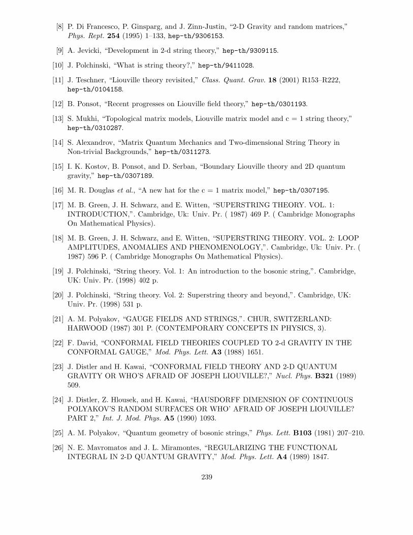
[8] P. Di Francesco, P. Ginsparg, and J. Zinn-Justin, “2-D Gravity and random matrices,”Phys. Rept. 254 (1995) 1–133, hep-th/9306153.
[9] A. Jevicki, “Development in 2-d string theory,” hep-th/9309115.
[10] J. Polchinski, “What is string theory?,” hep-th/9411028.
[11] J. Teschner, “Liouville theory revisited,” Class. Quant. Grav. 18 (2001) R153–R222,hep-th/0104158.
[12] B. Ponsot, “Recent progresses on Liouville field theory,” hep-th/0301193.
[13] S. Mukhi, “Topological matrix models, Liouville matrix model and c = 1 string theory,”hep-th/0310287.
[14] S. Alexandrov, “Matrix Quantum Mechanics and Two-dimensional String Theory inNon-trivial Backgrounds,” hep-th/0311273.
[15] I. K. Kostov, B. Ponsot, and D. Serban, “Boundary Liouville theory and 2D quantumgravity,” hep-th/0307189.
[16] M. R. Douglas et al., “A new hat for the c = 1 matrix model,” hep-th/0307195.
[17] M. B. Green, J. H. Schwarz, and E. Witten, “SUPERSTRING THEORY. VOL. 1:INTRODUCTION,”. Cambridge, Uk: Univ. Pr. ( 1987) 469 P. ( Cambridge MonographsOn Mathematical Physics).
[18] M. B. Green, J. H. Schwarz, and E. Witten, “SUPERSTRING THEORY. VOL. 2: LOOPAMPLITUDES, ANOMALIES AND PHENOMENOLOGY,”. Cambridge, Uk: Univ. Pr. (1987) 596 P. ( Cambridge Monographs On Mathematical Physics).
[19] J. Polchinski, “String theory. Vol. 1: An introduction to the bosonic string,”. Cambridge,UK: Univ. Pr. (1998) 402 p.
[20] J. Polchinski, “String theory. Vol. 2: Superstring theory and beyond,”. Cambridge, UK:Univ. Pr. (1998) 531 p.
[21] A. M. Polyakov, “GAUGE FIELDS AND STRINGS,”. CHUR, SWITZERLAND:HARWOOD (1987) 301 P. (CONTEMPORARY CONCEPTS IN PHYSICS, 3).
[22] F. David, “CONFORMAL FIELD THEORIES COUPLED TO 2-d GRAVITY IN THECONFORMAL GAUGE,” Mod. Phys. Lett. A3 (1988) 1651.
[23] J. Distler and H. Kawai, “CONFORMAL FIELD THEORY AND 2-D QUANTUMGRAVITY OR WHO’S AFRAID OF JOSEPH LIOUVILLE?,” Nucl. Phys. B321 (1989)509.
[24] J. Distler, Z. Hlousek, and H. Kawai, “HAUSDORFF DIMENSION OF CONTINUOUSPOLYAKOV’S RANDOM SURFACES OR WHO’ AFRAID OF JOSEPH LIOUVILLE?PART 2,” Int. J. Mod. Phys. A5 (1990) 1093.
[25] A. M. Polyakov, “Quantum geometry of bosonic strings,” Phys. Lett. B103 (1981) 207–210.
[26] N. E. Mavromatos and J. L. Miramontes, “REGULARIZING THE FUNCTIONALINTEGRAL IN 2-D QUANTUM GRAVITY,” Mod. Phys. Lett. A4 (1989) 1847.
239

[27] E. D’Hoker and P. S. Kurzepa, “2-D QUANTUM GRAVITY AND LIOUVILLETHEORY,” Mod. Phys. Lett. A5 (1990) 1411–1422.
[28] E. D’Hoker, “Equivalence of Liouville theory and 2-D quantum gravity,” Mod. Phys. Lett.
A6 (1991) 745–768.
[29] A. M. Polyakov, “The wall of the cave,” Int. J. Mod. Phys. A14 (1999) 645–658,hep-th/9809057.
[30] S. R. Das, S. Naik, and S. R. Wadia, “QUANTIZATION OF THE LIOUVILLE MODEAND STRING THEORY,” Mod. Phys. Lett. A4 (1989) 1033.
[31] D. Friedan, “NONLINEAR MODELS IN TWO epsilon DIMENSIONS,” Phys. Rev. Lett.
45 (1980) 1057.
[32] J. Callan, Curtis G., E. J. Martinec, M. J. Perry, and D. Friedan, “STRINGS INBACKGROUND FIELDS,” Nucl. Phys. B262 (1985) 593.
[33] E. S. Fradkin and A. A. Tseytlin, “EFFECTIVE FIELD THEORY FROM QUANTIZEDSTRINGS,” Phys. Lett. B158 (1985) 316.
[34] E. S. Fradkin and A. A. Tseytlin, “QUANTUM STRING THEORY EFFECTIVEACTION,” Nucl. Phys. B261 (1985) 1–27.
[35] A. A. Tseytlin, “ON THE STRUCTURE OF THE RENORMALIZATION GROUP BETAFUNCTIONS IN A CLASS OF TWO-DIMENSIONAL MODELS,” Phys. Lett. B241(1990) 233.
[36] T. L. Curtright and C. B. Thorn, “CONFORMALLY INVARIANT QUANTIZATION OFTHE LIOUVILLE THEORY,” Phys. Rev. Lett. 48 (1982) 1309.
[37] A. B. Zamolodchikov and A. B. Zamolodchikov, “Structure constants and conformalbootstrap in Liouville field theory,” Nucl. Phys. B477 (1996) 577–605, hep-th/9506136.
[38] E. D’Hoker and R. Jackiw, “LIOUVILLE FIELD THEORY,” Phys. Rev. D26 (1982) 3517.
[39] E. D’Hoker, D. Z. Freedman, and R. Jackiw, “SO(2,1) INVARIANT QUANTIZATION OFTHE LIOUVILLE THEORY,” Phys. Rev. D28 (1983) 2583.
[40] T. L. Curtright and G. I. Ghandour, “Using functional methods to compute quantum effectsin the Liouville model,” hep-th/9503080.
[41] V. G. Knizhnik, A. M. Polyakov, and A. B. Zamolodchikov, “Fractal structure of2d-quantum gravity,” Mod. Phys. Lett. A3 (1988) 819.
[42] J. Polchinski, “EVALUATION OF THE ONE LOOP STRING PATH INTEGRAL,”Commun. Math. Phys. 104 (1986) 37.
[43] A. Sen, “Rolling tachyon,” JHEP 04 (2002) 048, hep-th/0203211.
[44] E. Witten, “NONCOMMUTATIVE GEOMETRY AND STRING FIELD THEORY,” Nucl.
Phys. B268 (1986) 253.
[45] K. Ohmori, “A review on tachyon condensation in open string field theories,”hep-th/0102085.
240

[46] W. Taylor, “Lectures on D-branes, tachyon condensation, and string field theory,”hep-th/0301094.
[47] P.-J. De Smet, “Tachyon condensation: Calculations in string field theory,”hep-th/0109182.
[48] I. Y. Arefeva, D. M. Belov, A. A. Giryavets, A. S. Koshelev, and P. B. Medvedev,“Noncommutative field theories and (super)string field theories,” hep-th/0111208.
[49] A. A. Tseytlin, “Sigma model approach to string theory effective actions with tachyons,” J.
Math. Phys. 42 (2001) 2854–2871, hep-th/0011033.
[50] E. Witten, “On background independent open string field theory,” Phys. Rev. D46 (1992)5467–5473, hep-th/9208027.
[51] E. Witten, “Some computations in background independent off-shell string theory,” Phys.
Rev. D47 (1993) 3405–3410, hep-th/9210065.
[52] S. L. Shatashvili, “Comment on the background independent open string theory,” Phys.
Lett. B311 (1993) 83–86, hep-th/9303143.
[53] S. L. Shatashvili, “On the problems with background independence in string theory,”hep-th/9311177.
[54] D. Kutasov and V. Niarchos, “Tachyon effective actions in open string theory,” Nucl. Phys.
B666 (2003) 56–70, hep-th/0304045.
[55] B. H. Lian and G. J. Zuckerman, “New selection rules and physical states in 2-D gravity:Conformal gauge,” Phys. Lett. B254 (1991) 417–423.
[56] B. H. Lian and G. J. Zuckerman, “BRST cohomology and highest weight vectors. 1,”Commun. Math. Phys. 135 (1991) 547–580.
[57] B. H. Lian and G. J. Zuckerman, “2-D gravity with c = 1 matter,” Phys. Lett. B266 (1991)21–28.
[58] B. H. Lian and G. J. Zuckerman, “Semiinfinite homology and 2-D gravity. 1,” Commun.
Math. Phys. 145 (1992) 561–593.
[59] B. H. Lian and G. J. Zuckerman, “New perspectives on the BRST algebraic structure ofstring theory,” Commun. Math. Phys. 154 (1993) 613–646, hep-th/9211072.
[60] E. Witten, “Ground ring of two-dimensional string theory,” Nucl. Phys. B373 (1992)187–213, hep-th/9108004.
[61] E. Witten and B. Zwiebach, “Algebraic structures and differential geometry in 2 −D stringtheory,” Nucl. Phys. B377 (1992) 55–112, hep-th/9201056.
[62] P. Bouwknegt, J. G. McCarthy, and K. Pilch, “BRST analysis of physical states for 2-Dgravity coupled to c ¡= 1 matter,” Commun. Math. Phys. 145 (1992) 541–560.
[63] H. Ishikawa and M. Kato, “C = 1 string as a topological model,” Int. J. Mod. Phys. A9(1994) 5769–5790, hep-th/9304039.
241

[64] Y. Kazama and H. Nicolai, “On the exact operator formalism of two-dimensional Liouvillequantum gravity in Minkowski space-time,” Int. J. Mod. Phys. A9 (1994) 667–710,hep-th/9305023.
[65] I. R. Klebanov and A. Pasquinucci, “Correlation functions from two-dimensional stringward identities,” Nucl. Phys. B393 (1993) 261–279, hep-th/9204052.
[66] I. R. Klebanov and A. M. Polyakov, “Interaction of discrete states in two-dimensional stringtheory,” Mod. Phys. Lett. A6 (1991) 3273–3281, hep-th/9109032.
[67] N. Seiberg and D. Shih, “Branes, Rings and Matrix Models in Minimal (Super)stringTheory,” hep-th/0312170.
[68] O. Aharony, S. S. Gubser, J. M. Maldacena, H. Ooguri, and Y. Oz, “Large N field theories,string theory and gravity,” Phys. Rept. 323 (2000) 183–386, hep-th/9905111.
[69] A. M. Polyakov, “Gauge fields and space-time,” Int. J. Mod. Phys. A17S1 (2002) 119–136,hep-th/0110196.
[70] E. D’Hoker and D. Z. Freedman, “Supersymmetric gauge theories and the AdS/CFTcorrespondence,” hep-th/0201253.
[71] J. Maldacena, “Les Houches lectures on large N field theories and gravity,”. Prepared forLes Houches Summer School: Session 76: Euro Summer School on Unity of FundamentalPhysics: Gravity, Gauge Theory and Strings, Les Houches, France, 30 Jul - 31 Aug 2001.
[72] I. R. Klebanov, “TASI lectures: Introduction to the AdS/CFT correspondence,”hep-th/0009139.
[73] J. M. Maldacena, “The large N limit of superconformal field theories and supergravity,”Adv. Theor. Math. Phys. 2 (1998) 231–252, hep-th/9711200.
[74] S. S. Gubser, I. R. Klebanov, and A. M. Polyakov, “Gauge theory correlators fromnon-critical string theory,” Phys. Lett. B428 (1998) 105–114, hep-th/9802109.
[75] E. Witten, “Anti-de Sitter space and holography,” Adv. Theor. Math. Phys. 2 (1998)253–291, hep-th/9802150.
[76] R. Gopakumar, “Lecture at Komaba campus, university of Tokyo,”.
[77] R. Gopakumar and C. Vafa, “On the gauge theory/geometry correspondence,” Adv. Theor.
Math. Phys. 3 (1999) 1415–1443, hep-th/9811131.
[78] H. Ooguri and C. Vafa, “Worldsheet derivation of a large N duality,” Nucl. Phys. B641(2002) 3–34, hep-th/0205297.
[79] N. Berkovits, H. Ooguri, and C. Vafa, “On the worldsheet derivation of large N dualities forthe superstring,” hep-th/0310118.
[80] A. Giveon, D. Kutasov, and O. Pelc, “Holography for non-critical superstrings,” JHEP 10(1999) 035, hep-th/9907178.
[81] J. McGreevy and H. Verlinde, “Strings from tachyons: The c = 1 matrix reloated,”hep-th/0304224.
242
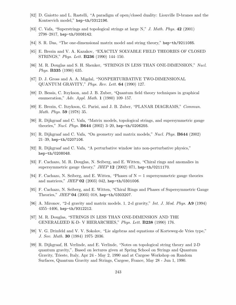
[82] D. Gaiotto and L. Rastelli, “A paradigm of open/closed duality: Liouville D-branes and theKontsevich model,” hep-th/0312196.
[83] C. Vafa, “Superstrings and topological strings at large N,” J. Math. Phys. 42 (2001)2798–2817, hep-th/0008142.
[84] S. R. Das, “The one-dimensional matrix model and string theory,” hep-th/9211085.
[85] E. Brezin and V. A. Kazakov, “EXACTLY SOLVABLE FIELD THEORIES OF CLOSEDSTRINGS,” Phys. Lett. B236 (1990) 144–150.
[86] M. R. Douglas and S. H. Shenker, “STRINGS IN LESS THAN ONE-DIMENSION,” Nucl.
Phys. B335 (1990) 635.
[87] D. J. Gross and A. A. Migdal, “NONPERTURBATIVE TWO-DIMENSIONALQUANTUM GRAVITY,” Phys. Rev. Lett. 64 (1990) 127.
[88] D. Bessis, C. Itzykson, and J. B. Zuber, “Quantum field theory techniques in graphicalenumeration,” Adv. Appl. Math. 1 (1980) 109–157.
[89] E. Brezin, C. Itzykson, G. Parisi, and J. B. Zuber, “PLANAR DIAGRAMS,” Commun.
Math. Phys. 59 (1978) 35.
[90] R. Dijkgraaf and C. Vafa, “Matrix models, topological strings, and supersymmetric gaugetheories,” Nucl. Phys. B644 (2002) 3–20, hep-th/0206255.
[91] R. Dijkgraaf and C. Vafa, “On geometry and matrix models,” Nucl. Phys. B644 (2002)21–39, hep-th/0207106.
[92] R. Dijkgraaf and C. Vafa, “A perturbative window into non-perturbative physics,”hep-th/0208048.
[93] F. Cachazo, M. R. Douglas, N. Seiberg, and E. Witten, “Chiral rings and anomalies insupersymmetric gauge theory,” JHEP 12 (2002) 071, hep-th/0211170.
[94] F. Cachazo, N. Seiberg, and E. Witten, “Phases of N = 1 supersymmetric gauge theoriesand matrices,” JHEP 02 (2003) 042, hep-th/0301006.
[95] F. Cachazo, N. Seiberg, and E. Witten, “Chiral Rings and Phases of Supersymmetric GaugeTheories,” JHEP 04 (2003) 018, hep-th/0303207.
[96] A. Mironov, “2-d gravity and matrix models. 1. 2-d gravity,” Int. J. Mod. Phys. A9 (1994)4355–4406, hep-th/9312212.
[97] M. R. Douglas, “STRINGS IN LESS THAN ONE-DIMENSION AND THEGENERALIZED K-D- V HIERARCHIES,” Phys. Lett. B238 (1990) 176.
[98] V. G. Drinfeld and V. V. Sokolov, “Lie algebras and equations of Korteweg-de Vries type,”J. Sov. Math. 30 (1984) 1975–2036.
[99] R. Dijkgraaf, H. Verlinde, and E. Verlinde, “Notes on topological string theory and 2-Dquantum gravity,”. Based on lectures given at Spring School on Strings and QuantumGravity, Trieste, Italy, Apr 24 - May 2, 1990 and at Cargese Workshop on RandomSurfaces, Quantum Gravity and Strings, Cargese, France, May 28 - Jun 1, 1990.
243
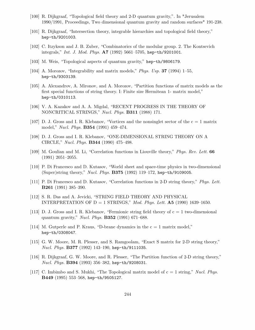
[100] R. Dijkgraaf, “Topological field theory and 2-D quantum gravity,”. In *Jerusalem1990/1991, Proceedings, Two dimensional quantum gravity and random surfaces* 191-238.
[101] R. Dijkgraaf, “Intersection theory, integrable hierarchies and topological field theory,”hep-th/9201003.
[102] C. Itzykson and J. B. Zuber, “Combinatorics of the modular group. 2. The Kontsevichintegrals,” Int. J. Mod. Phys. A7 (1992) 5661–5705, hep-th/9201001.
[103] M. Weis, “Topological aspects of quantum gravity,” hep-th/9806179.
[104] A. Morozov, “Integrability and matrix models,” Phys. Usp. 37 (1994) 1–55,hep-th/9303139.
[105] A. Alexandrov, A. Mironov, and A. Morozov, “Partition functions of matrix models as thefirst special functions of string theory. I: Finite size Hermitean 1- matrix model,”hep-th/0310113.
[106] V. A. Kazakov and A. A. Migdal, “RECENT PROGRESS IN THE THEORY OFNONCRITICAL STRINGS,” Nucl. Phys. B311 (1988) 171.
[107] D. J. Gross and I. R. Klebanov, “Vortices and the nonsinglet sector of the c = 1 matrixmodel,” Nucl. Phys. B354 (1991) 459–474.
[108] D. J. Gross and I. R. Klebanov, “ONE-DIMENSIONAL STRING THEORY ON ACIRCLE,” Nucl. Phys. B344 (1990) 475–498.
[109] M. Goulian and M. Li, “Correlation functions in Liouville theory,” Phys. Rev. Lett. 66(1991) 2051–2055.
[110] P. Di Francesco and D. Kutasov, “World sheet and space-time physics in two-dimensional(Super)string theory,” Nucl. Phys. B375 (1992) 119–172, hep-th/9109005.
[111] P. Di Francesco and D. Kutasov, “Correlation functions in 2-D string theory,” Phys. Lett.
B261 (1991) 385–390.
[112] S. R. Das and A. Jevicki, “STRING FIELD THEORY AND PHYSICALINTERPRETATION OF D = 1 STRINGS,” Mod. Phys. Lett. A5 (1990) 1639–1650.
[113] D. J. Gross and I. R. Klebanov, “Fermionic string field theory of c = 1 two-dimensionalquantum gravity,” Nucl. Phys. B352 (1991) 671–688.
[114] M. Gutperle and P. Kraus, “D-brane dynamics in the c = 1 matrix model,”hep-th/0308047.
[115] G. W. Moore, M. R. Plesser, and S. Ramgoolam, “Exact S matrix for 2-D string theory,”Nucl. Phys. B377 (1992) 143–190, hep-th/9111035.
[116] R. Dijkgraaf, G. W. Moore, and R. Plesser, “The Partition function of 2-D string theory,”Nucl. Phys. B394 (1993) 356–382, hep-th/9208031.
[117] C. Imbimbo and S. Mukhi, “The Topological matrix model of c = 1 string,” Nucl. Phys.
B449 (1995) 553–568, hep-th/9505127.
244

[118] M. Kontsevich, “Intersection theory on the moduli space of curves and the matrix Airyfunction,” Commun. Math. Phys. 147 (1992) 1–23.
[119] R. Penner, “Perturbative series and the moduli space of Riemann surfaces,”.
[120] J. Distler and C. Vafa, “A Critical matrix model at c = 1,” Mod. Phys. Lett. A6 (1991)259–270.
[121] S. Y. Alexandrov, V. A. Kazakov, and I. K. Kostov, “2D string theory as normal matrixmodel,” Nucl. Phys. B667 (2003) 90–110, hep-th/0302106.
[122] M. Aganagic, R. Dijkgraaf, A. Klemm, M. Marino, and C. Vafa, “Topological strings andintegrable hierarchies,” hep-th/0312085.
[123] H. Dorn and H. J. Otto, “Two and three point functions in Liouville theory,” Nucl. Phys.
B429 (1994) 375–388, hep-th/9403141.
[124] J. Teschner, “On the Liouville three point function,” Phys. Lett. B363 (1995) 65–70,hep-th/9507109.
[125] M. A. Shifman and A. I. Vainshtein, “Instantons versus supersymmetry: Fifteen yearslater,” hep-th/9902018.
[126] N. Dorey, T. J. Hollowood, V. V. Khoze, and M. P. Mattis, “The calculus of manyinstantons,” Phys. Rept. 371 (2002) 231–459, hep-th/0206063.
[127] V. S. Dotsenko and V. A. Fateev, “Conformal algebra and multipoint correlation functionsin 2D statistical models,” Nucl. Phys. B240 (1984) 312.
[128] V. S. Dotsenko and V. A. Fateev, “FOUR POINT CORRELATION FUNCTIONS ANDTHE OPERATOR ALGEBRA IN THE two-dimensional CONFORMAL INVARIANTTHEORIES WITH THE CENTRAL CHARGE C ¡ 1,” Nucl. Phys. B251 (1985) 691.
[129] J. J. L. Lutzen, “Master of pure and applied mathematics,”.
[130] J. M. Maldacena, H. Ooguri, and J. Son, “Strings in AdS(3) and the SL(2,R) WZW model.II: Euclidean black hole,” J. Math. Phys. 42 (2001) 2961–2977, hep-th/0005183.
[131] B. Ponsot, V. Schomerus, and J. Teschner, “Branes in the Euclidean AdS(3),” JHEP 02(2002) 016, hep-th/0112198.
[132] V. G. Kac, “CONTRAVARIANT FORM FOR INFINITE DIMENSIONAL LIEALGEBRAS AND SUPERALGEBRAS. (TALK),”. In *Austin 1978, Proceedings, GroupTheoretical Methods In Physics*, Berlin 1979, 441-445.
[133] B. L. Feigin and D. B. Fuchs, “VERMA MODULES OVER THE VIRASOROALGEBRA,”. PREPRINT - FEIGIN, B.L. (REC.OCT.88) 16p.
[134] L. O’Raifeartaigh, J. M. Pawlowski, and V. V. Sreedhar, “The duality of quantum Liouvillefield theory,” Annals Phys. 277 (1999) 117–143, hep-th/9811090.
[135] L. O’Raifeartaigh and V. V. Sreedhar, “Duality in Liouville theory as a reduced symmetry,”Phys. Lett. B461 (1999) 66–70, hep-th/9906116.
245
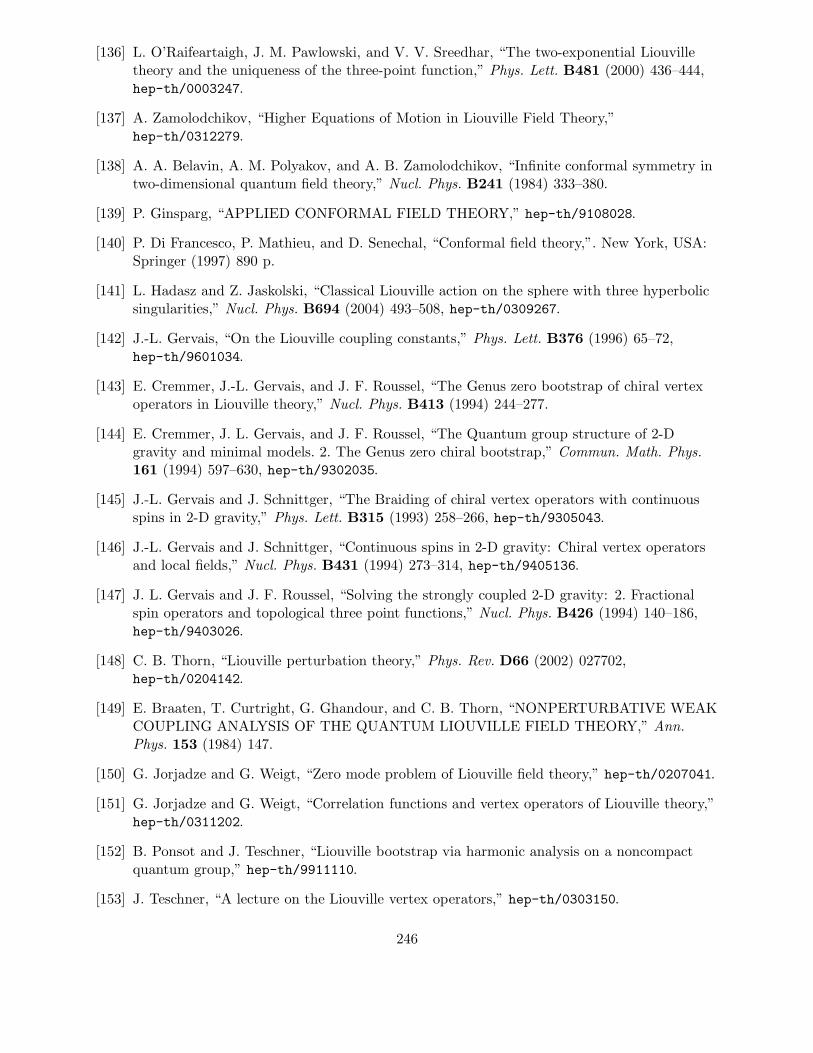
[136] L. O’Raifeartaigh, J. M. Pawlowski, and V. V. Sreedhar, “The two-exponential Liouvilletheory and the uniqueness of the three-point function,” Phys. Lett. B481 (2000) 436–444,hep-th/0003247.
[137] A. Zamolodchikov, “Higher Equations of Motion in Liouville Field Theory,”hep-th/0312279.
[138] A. A. Belavin, A. M. Polyakov, and A. B. Zamolodchikov, “Infinite conformal symmetry intwo-dimensional quantum field theory,” Nucl. Phys. B241 (1984) 333–380.
[139] P. Ginsparg, “APPLIED CONFORMAL FIELD THEORY,” hep-th/9108028.
[140] P. Di Francesco, P. Mathieu, and D. Senechal, “Conformal field theory,”. New York, USA:Springer (1997) 890 p.
[141] L. Hadasz and Z. Jaskolski, “Classical Liouville action on the sphere with three hyperbolicsingularities,” Nucl. Phys. B694 (2004) 493–508, hep-th/0309267.
[142] J.-L. Gervais, “On the Liouville coupling constants,” Phys. Lett. B376 (1996) 65–72,hep-th/9601034.
[143] E. Cremmer, J.-L. Gervais, and J. F. Roussel, “The Genus zero bootstrap of chiral vertexoperators in Liouville theory,” Nucl. Phys. B413 (1994) 244–277.
[144] E. Cremmer, J. L. Gervais, and J. F. Roussel, “The Quantum group structure of 2-Dgravity and minimal models. 2. The Genus zero chiral bootstrap,” Commun. Math. Phys.
161 (1994) 597–630, hep-th/9302035.
[145] J.-L. Gervais and J. Schnittger, “The Braiding of chiral vertex operators with continuousspins in 2-D gravity,” Phys. Lett. B315 (1993) 258–266, hep-th/9305043.
[146] J.-L. Gervais and J. Schnittger, “Continuous spins in 2-D gravity: Chiral vertex operatorsand local fields,” Nucl. Phys. B431 (1994) 273–314, hep-th/9405136.
[147] J. L. Gervais and J. F. Roussel, “Solving the strongly coupled 2-D gravity: 2. Fractionalspin operators and topological three point functions,” Nucl. Phys. B426 (1994) 140–186,hep-th/9403026.
[148] C. B. Thorn, “Liouville perturbation theory,” Phys. Rev. D66 (2002) 027702,hep-th/0204142.
[149] E. Braaten, T. Curtright, G. Ghandour, and C. B. Thorn, “NONPERTURBATIVE WEAKCOUPLING ANALYSIS OF THE QUANTUM LIOUVILLE FIELD THEORY,” Ann.
Phys. 153 (1984) 147.
[150] G. Jorjadze and G. Weigt, “Zero mode problem of Liouville field theory,” hep-th/0207041.
[151] G. Jorjadze and G. Weigt, “Correlation functions and vertex operators of Liouville theory,”hep-th/0311202.
[152] B. Ponsot and J. Teschner, “Liouville bootstrap via harmonic analysis on a noncompactquantum group,” hep-th/9911110.
[153] J. Teschner, “A lecture on the Liouville vertex operators,” hep-th/0303150.
246

[154] S.-i. Yamaguchi, “Logarithmic correlation functions in Liouville field theory,” Phys. Lett.
B546 (2002) 300–304, hep-th/0209146.
[155] J. Teschner, “Remarks on Liouville theory with boundary,” hep-th/0009138.
[156] K. Hosomichi, “Bulk-boundary propagator in Liouville theory on a disc,” JHEP 11 (2001)044, hep-th/0108093.
[157] B. Ponsot and J. Teschner, “Boundary Liouville field theory: Boundary three pointfunction,” Nucl. Phys. B622 (2002) 309–327, hep-th/0110244.
[158] N. Ishibashi, “THE BOUNDARY AND CROSSCAP STATES IN CONFORMAL FIELDTHEORIES,” Mod. Phys. Lett. A4 (1989) 251.
[159] E. J. Martinec, “The annular report on non-critical string theory,” hep-th/0305148.
[160] J. Teschner, “On boundary perturbations in Liouville theory and brane dynamics innoncritical string theories,” hep-th/0308140.
[161] I. R. Klebanov, J. Maldacena, and N. Seiberg, “Unitary and complex matrix models as 1-dtype 0 strings,” hep-th/0309168.
[162] M. Asano and M. Natsuume, “The no-ghost theorem for string theory in curvedbackgrounds with a flat timelike direction,” Nucl. Phys. B588 (2000) 453–470,hep-th/0005002.
[163] M. Asano and M. Natsuume, “The no-ghost theorem in curved backgrounds with a timelikeu(1): NSR string,” Nucl. Phys. B672 (2003) 39–63, hep-th/0303051.
[164] B. Ponsot, “Liouville theory on the pseudosphere: Bulk-boundary structure constant,”hep-th/0309211.
[165] J. L. Cardy, “CONFORMAL INVARIANCE AND SURFACE CRITICAL BEHAVIOR,”Nucl. Phys. B240 (1984) 514–532.
[166] J. L. Cardy, “EFFECT OF BOUNDARY CONDITIONS ON THE OPERATORCONTENT OF TWO-DIMENSIONAL CONFORMALLY INVARIANT THEORIES,”Nucl. Phys. B275 (1986) 200–218.
[167] J. L. Cardy, “BOUNDARY CONDITIONS, FUSION RULES AND THE VERLINDEFORMULA,” Nucl. Phys. B324 (1989) 581.
[168] I. K. Kostov, “THE ADE FACE MODELS ON A FLUCTUATING PLANAR LATTICE,”Nucl. Phys. B326 (1989) 583.
[169] I. K. Kostov, “Loop amplitudes for nonrational string theories,” Phys. Lett. B266 (1991)317–324.
[170] I. K. Kostov, “Strings with discrete target space,” Nucl. Phys. B376 (1992) 539–598,hep-th/9112059.
[171] I. K. Kostov, “Boundary correlators in 2D quantum gravity: Liouville versus discreteapproach,” Nucl. Phys. B658 (2003) 397–416, hep-th/0212194.
247
[172] E. D’Hoker and R. Jackiw, “SPACE TRANSLATION BREAKING ANDCOMPACTIFICATION IN THE LIOUVILLE THEORY,” Phys. Rev. Lett. 50 (1983)1719–1722.
[173] P. Menotti and E. Tonni, “The tetrahedron graph in Liouville theory on the pseudosphere,”hep-th/0311234.
[174] T. Takayanagi and N. Toumbas, “A matrix model dual of type 0B string theory in twodimensions,” JHEP 07 (2003) 064, hep-th/0307083.
[175] I. R. Klebanov, J. Maldacena, and N. Seiberg, “D-brane decay in two-dimensional stringtheory,” JHEP 07 (2003) 045, hep-th/0305159.
[176] J. McGreevy, J. Teschner, and H. Verlinde, “Classical and quantum D-branes in 2D stringtheory,” hep-th/0305194.
[177] A. Sen, “Open-closed duality: Lessons from matrix model,” hep-th/0308068.
[178] G. Mandal and S. R. Wadia, “Rolling tachyon solution of two-dimensional string theory,”hep-th/0312192.
[179] A. Sen, “Tachyon matter,” JHEP 07 (2002) 065, hep-th/0203265.
[180] Z. Yang, “Dynamical loops in D = 1 random matrix models,” Phys. Lett. B257 (1991)40–44.
[181] J. A. Minahan, “Matrix models and one-dimensional open string theory,” Int. J. Mod. Phys.
A8 (1993) 3599–3614, hep-th/9204013.
[182] V. A. Kazakov and I. K. Kostov, “Loop gas model for open strings,” Nucl. Phys. B386(1992) 520–557, hep-th/9205059.
[183] J. Avan and A. Jevicki, “Collective field theory of the matrix-vector models,” Nucl. Phys.
B469 (1996) 287–301, hep-th/9512147.
[184] J. Avan, A. Jevicki, and J. Lee, “Yangian-invariant field theory of matrix-vector models,”Nucl. Phys. B486 (1997) 650–672, hep-th/9607083.
[185] M. Gutperle and A. Strominger, “Timelike boundary Liouville theory,” Phys. Rev. D67(2003) 126002, hep-th/0301038.
[186] N. R. Constable and F. Larsen, “The rolling tachyon as a matrix model,” JHEP 06 (2003)017, hep-th/0305177.
[187] W. Fischler and L. Susskind, “DILATON TADPOLES, STRING CONDENSATES ANDSCALE INVARIANCE,” Phys. Lett. B171 (1986) 383.
[188] W. Fischler and L. Susskind, “DILATON TADPOLES, STRING CONDENSATES ANDSCALE INVARIANCE. 2,” Phys. Lett. B173 (1986) 262.
[189] A. Strominger and T. Takayanagi, “Correlators in timelike bulk Liouville theory,” Adv.
Theor. Math. Phys. 7 (2003) 369–379, hep-th/0303221.
[190] V. Schomerus, “Rolling tachyons from Liouville theory,” JHEP 11 (2003) 043,hep-th/0306026.
248

[191] I. Runkel and G. M. T. Watts, “A non-rational CFT with central charge 1,” Fortsch. Phys.
50 (2002) 959–965, hep-th/0201231.
[192] E. Witten, “TOPOLOGICAL SIGMA MODELS,” Commun. Math. Phys. 118 (1988) 411.
[193] E. Witten, “Phases of N = 2 theories in two dimensions,” Nucl. Phys. B403 (1993)159–222, hep-th/9301042.
[194] C. Vafa, “Topological Landau-Ginzburg models,” Mod. Phys. Lett. A6 (1991) 337–346.
[195] D. Ghoshal and S. Mukhi, “Topological Landau-Ginzburg model of two-dimensional stringtheory,” Nucl. Phys. B425 (1994) 173–190, hep-th/9312189.
[196] D. Ghoshal, C. Imbimbo, and S. Mukhi, “Topological 2-D string theory: Higher genusamplitudes and W(infinity) identities,” Nucl. Phys. B440 (1995) 355–372, hep-th/9410034.
[197] E. Witten, “TOPOLOGICAL GRAVITY,” Phys. Lett. B206 (1988) 601.
[198] J. M. F. Labastida, M. Pernici, and E. Witten, “TOPOLOGICAL GRAVITY INTWO-DIMENSIONS,” Nucl. Phys. B310 (1988) 611.
[199] D. Ghoshal and C. Vafa, “C = 1 string as the topological theory of the conifold,” Nucl.
Phys. B453 (1995) 121–128, hep-th/9506122.
[200] R. Gopakumar and C. Vafa, “Topological gravity as large N topological gauge theory,” Adv.
Theor. Math. Phys. 2 (1998) 413–442, hep-th/9802016.
[201] R. Gopakumar and C. Vafa, “M-theory and topological strings. I,” hep-th/9809187.
[202] R. Gopakumar and C. Vafa, “M-theory and topological strings. II,” hep-th/9812127.
[203] E. Witten, “Chern-Simons gauge theory as a string theory,” Prog. Math. 133 (1995)637–678, hep-th/9207094.
[204] G. Macdonald, I, “The volume of a comlact Lie group,” Invent. Math. 56 (1980) 563.
[205] M. Marino, “Chern-Simons theory, matrix integrals, and perturbative three-manifoldinvariants,” hep-th/0207096.
[206] M. Aganagic, A. Klemm, M. Marino, and C. Vafa, “Matrix model as a mirror ofChern-Simons theory,” hep-th/0211098.
[207] J. de Boer, A. Sinkovics, E. Verlinde, and J.-T. Yee, “String interactions in c = 1 matrixmodel,” hep-th/0312135.
[208] A. Boyarsky, B. Kulik, and O. Ruchayskiy, “Classical and Quantum Branes in c=1 StringTheory and Quantum Hall Effect,” hep-th/0312242.
[209] N. Lambert, H. Liu, and J. Maldacena, “Closed strings from decaying D-branes,”hep-th/0303139.
[210] J. L. Karczmarek, H. Liu, J. Maldacena, and A. Strominger, “UV finite brane decay,” JHEP
11 (2003) 042, hep-th/0306132.
[211] A. Strominger, “Open string creation by S-branes,” hep-th/0209090.
249
[212] F. Larsen, A. Naqvi, and S. Terashima, “Rolling tachyons and decaying branes,” JHEP 02(2003) 039, hep-th/0212248.
[213] S. R. Das, “D branes in 2d string theory and classical limits,” hep-th/0401067.
[214] J. Ambjorn and R. A. Janik, “The decay of quantum D-branes,” hep-th/0312163.
[215] E. Witten, “On string theory and black holes,” Phys. Rev. D44 (1991) 314–324.
[216] R. Dijkgraaf, H. Verlinde, and E. Verlinde, “String propagation in a black hole geometry,”Nucl. Phys. B371 (1992) 269–314.
[217] M. Bershadsky and D. Kutasov, “Comment on gauged WZW theory,” Phys. Lett. B266(1991) 345–352.
[218] T. Eguchi, H. Kanno, and S.-K. Yang, “W(infinity) algebra in two-dimensional black hole,”Phys. Lett. B298 (1993) 73–78, hep-th/9209122.
[219] V. Fateev, A. B. Zamolodchikov, and A. B. Zamolodchikov, “unpublished,”.
[220] V. Kazakov, I. K. Kostov, and D. Kutasov, “A matrix model for the two-dimensional blackhole,” Nucl. Phys. B622 (2002) 141–188, hep-th/0101011.
[221] T. Fukuda and K. Hosomichi, “Three-point functions in sine-Liouville theory,” JHEP 09(2001) 003, hep-th/0105217.
[222] S. Ribault and V. Schomerus, “Branes in the 2-D black hole,” hep-th/0310024.
[223] S. L. Lukyanov, E. S. Vitchev, and A. B. Zamolodchikov, “Integrable model of boundaryinteraction: The paperclip,” Nucl. Phys. B683 (2004) 423–454, hep-th/0312168.
[224] S. Y. Alexandrov, V. A. Kazakov, and D. Kutasov, “Non-perturbative effects in matrixmodels and D-branes,” JHEP 09 (2003) 057, hep-th/0306177.
[225] S. Alexandrov, “(m,n) ZZ branes and the c = 1 matrix model,” hep-th/0310135.
[226] F. David, “Phases of the large N matrix model and nonperturbative effects in 2-d gravity,”Nucl. Phys. B348 (1991) 507–524.
[227] F. David, “Nonperturbative effects in matrix models and vacua of two- dimensionalgravity,” Phys. Lett. B302 (1993) 403–410, hep-th/9212106.
[228] B. Eynard and J. Zinn-Justin, “Large order behavior of 2-D gravity coupled to d ¡ 1matter,” Phys. Lett. B302 (1993) 396–402, hep-th/9301004.
[229] S. H. Shenker, “The Strength of nonperturbative effects in string theory,”. Presented at theCargese Workshop on Random Surfaces, Quantum Gravity and Strings, Cargese, France,May 28 - Jun 1, 1990.
[230] J. Polchinski, “Combinatorics of boundaries in string theory,” Phys. Rev. D50 (1994)6041–6045, hep-th/9407031.
[231] D. Kutasov, E. J. Martinec, and N. Seiberg, “Ground rings and their modules in 2-Dgravity with c ¡= 1 matter,” Phys. Lett. B276 (1992) 437–444, hep-th/9111048.
250

[232] I. K. Kostov, “Boundary Ground Ring in 2D String Theory,” hep-th/0312301.
[233] A. A. Tseytlin, “On the form of the black hole solution in D = 2 theory,” Phys. Lett. B268(1991) 175–178.
[234] N. Seiberg and S. H. Shenker, “A Note on background (in)dependence,” Phys. Rev. D45(1992) 4581–4587, hep-th/9201017.
[235] I. Jack, D. R. T. Jones, and J. Panvel, “Exact bosonic and supersymmetric string black holesolutions,” Nucl. Phys. B393 (1993) 95–110, hep-th/9201039.
[236] K. Becker and M. Becker, “Interactions in the SL(2,IR) / U(1) black hole background,”Nucl. Phys. B418 (1994) 206–230, hep-th/9310046.
[237] E. Witten, “Two-dimensional string theory and black holes,” hep-th/9206069.
[238] K. Becker, “Strings, black holes and conformal field theory,” hep-th/9404157.
[239] Y. Kazama, “On quantum black holes,” hep-th/9412224.
[240] D. Grumiller, W. Kummer, and D. V. Vassilevich, “Dilaton gravity in two dimensions,”Phys. Rept. 369 (2002) 327–430, hep-th/0204253.
[241] D. Boulatov and V. Kazakov, “One-dimensional string theory with vortices as the upsidedown matrix oscillator,” Int. J. Mod. Phys. A8 (1993) 809–852, hep-th/0012228.
[242] G. W. Moore, “Gravitational phase transitions and the Sine-Gordon model,”hep-th/9203061.
[243] E. Hsu and D. Kutasov, “The Gravitational Sine-Gordon model,” Nucl. Phys. B396 (1993)693–707, hep-th/9212023.
[244] S. Mukhi and C. Vafa, “Two-dimensional black hole as a topological coset model of c = 1string theory,” Nucl. Phys. B407 (1993) 667–705, hep-th/9301083.
[245] I. Bars, C. Deliduman, and D. Minic, “String theory on AdS(3) revisited,” hep-th/9907087.
[246] D. Berenstein and R. G. Leigh, “Spacetime supersymmetry in AdS(3) backgrounds,” Phys.
Lett. B458 (1999) 297–303, hep-th/9904040.
[247] A. Giveon and M. Rocek, “Supersymmetric string vacua on AdS(3) x N,” JHEP 04 (1999)019, hep-th/9904024.
[248] Y. Sugawara, “Topological string on AdS(3) x N,” Nucl. Phys. B576 (2000) 265–284,hep-th/9909146.
[249] P. M. Petropoulos, “String theory on AdS(3): Some open questions,” hep-th/9908189.
[250] J. Teschner, “Operator product expansion and factorization in the H-3+ WZNW model,”Nucl. Phys. B571 (2000) 555–582, hep-th/9906215.
[251] J. M. Maldacena and H. Ooguri, “Strings in AdS(3) and SL(2,R) WZW model. I,” J. Math.
Phys. 42 (2001) 2929–2960, hep-th/0001053.
251

[252] A. Kato and Y. Satoh, “Modular invariance of string theory on AdS(3),” Phys. Lett. B486(2000) 306–313, hep-th/0001063.
[253] N. Ishibashi, K. Okuyama, and Y. Satoh, “Path integral approach to string theory onAdS(3),” Nucl. Phys. B588 (2000) 149–177, hep-th/0005152.
[254] K. Hosomichi, K. Okuyama, and Y. Satoh, “Free field approach to string theory onAdS(3),” Nucl. Phys. B598 (2001) 451–466, hep-th/0009107.
[255] A. L. Larsen and N. Sanchez, “Quantum coherent string states in AdS(3) and SL(2,R)WZWN model,” Phys. Rev. D62 (2000) 046003, hep-th/0001180.
[256] J. M. Maldacena and H. Ooguri, “Strings in AdS(3) and the SL(2,R) WZW model. III:Correlation functions,” Phys. Rev. D65 (2002) 106006, hep-th/0111180.
[257] Y. Satoh, “Three-point functions and operator product expansion in the SL(2) conformalfield theory,” Nucl. Phys. B629 (2002) 188–208, hep-th/0109059.
[258] K. Hosomichi and Y. Satoh, “Operator product expansion in string theory on AdS(3),”Mod. Phys. Lett. A17 (2002) 683–693, hep-th/0105283.
[259] G. Giribet and C. Nunez, “Correlators in AdS(3) string theory,” JHEP 06 (2001) 010,hep-th/0105200.
[260] A. Giveon and D. Kutasov, “Notes on AdS(3),” Nucl. Phys. B621 (2002) 303–336,hep-th/0106004.
[261] A. Giveon, D. Kutasov, and A. Schwimmer, “Comments on D-branes in AdS(3),” Nucl.
Phys. B615 (2001) 133–168, hep-th/0106005.
[262] A. Parnachev and D. A. Sahakyan, “Some remarks on D-branes in AdS(3),” JHEP 10(2001) 022, hep-th/0109150.
[263] P. Lee, H. Ooguri, and J.-w. Park, “Boundary states for AdS(2) branes in AdS(3),” Nucl.
Phys. B632 (2002) 283–302, hep-th/0112188.
[264] A. Sen, “Field theory of tachyon matter,” Mod. Phys. Lett. A17 (2002) 1797–1804,hep-th/0204143.
[265] M. Gutperle and A. Strominger, “Spacelike branes,” JHEP 04 (2002) 018, hep-th/0202210.
[266] A. Sen, “Time evolution in open string theory,” JHEP 10 (2002) 003, hep-th/0207105.
[267] P. Mukhopadhyay and A. Sen, “Decay of unstable D-branes with electric field,” JHEP 11(2002) 047, hep-th/0208142.
[268] A. Sen, “Time and tachyon,” Int. J. Mod. Phys. A18 (2003) 4869–4888, hep-th/0209122.
[269] A. Maloney, A. Strominger, and X. Yin, “S-brane thermodynamics,” JHEP 10 (2003) 048,hep-th/0302146.
[270] B. Chen, M. Li, and F.-L. Lin, “Gravitational radiation of rolling tachyon,” JHEP 11(2002) 050, hep-th/0209222.
252

[271] S.-J. Rey and S. Sugimoto, “Rolling tachyon with electric and magnetic fields: T- dualityapproach,” Phys. Rev. D67 (2003) 086008, hep-th/0301049.
[272] N. Moeller and B. Zwiebach, “Dynamics with infinitely many time derivatives and rollingtachyons,” JHEP 10 (2002) 034, hep-th/0207107.
[273] S. Sugimoto and S. Terashima, “Tachyon matter in boundary string field theory,” JHEP 07(2002) 025, hep-th/0205085.
[274] J. A. Minahan, “Rolling the tachyon in super BSFT,” JHEP 07 (2002) 030,hep-th/0205098.
[275] J. Kluson, “Time dependent solution in open bosonic string field theory,” hep-th/0208028.
[276] J. Kluson, “Exact solutions in open bosonic string field theory and marginal deformation inCFT,” hep-th/0209255.
[277] T. Okuda and S. Sugimoto, “Coupling of rolling tachyon to closed strings,” Nucl. Phys.
B647 (2002) 101–116, hep-th/0208196.
[278] I. Y. Aref’eva, L. V. Joukovskaya, and A. S. Koshelev, “Time evolution in superstring fieldtheory on non-BPS brane. I: Rolling tachyon and energy-momentum conservation,” JHEP
09 (2003) 012, hep-th/0301137.
[279] A. Ishida and S. Uehara, “Rolling down to D-brane and tachyon matter,” JHEP 02 (2003)050, hep-th/0301179.
[280] D. Gaiotto, N. Itzhaki, and L. Rastelli, “Closed strings as imaginary D-branes,”hep-th/0304192.
[281] Y. Demasure and R. A. Janik, “Backreaction and the rolling tachyon: An effective actionpoint of view,” hep-th/0305191.
[282] J. Kluson, “Particle production on half S-brane,” hep-th/0306002.
[283] J. Kluson, “The Schroedinger wave functional and S-branes,” Class. Quant. Grav. 20 (2003)4285–4304, hep-th/0307079.
[284] K. Nagami, “Closed string emission from unstable D-brane with background electric field,”hep-th/0309017.
[285] J. Kluson, “Note on D-brane effective action in the linear dilaton background,” JHEP 11(2003) 068, hep-th/0310066.
[286] S. Dasgupta and T. Dasgupta, “Renormalization group approach to c = 1 matrix model ona circle and D-brane decay,” hep-th/0310106.
[287] S. Dasgupta and T. Dasgupta, “Nonsinglet sector of c = 1 matrix model and 2D blackhole,” hep-th/0311177.
[288] K. Nagami, “Rolling tachyon with electromagnetic field in linear dilaton background,”hep-th/0312149.
[289] S. Y. Alexandrov, V. A. Kazakov, and I. K. Kostov, “Time-dependent backgrounds of 2Dstring theory,” Nucl. Phys. B640 (2002) 119–144, hep-th/0205079.
253
[290] I. K. Kostov, “Integrable flows in c = 1 string theory,” J. Phys. A36 (2003) 3153–3172,hep-th/0208034.
[291] S. Alexandrov, “Backgrounds of 2D string theory from matrix model,” hep-th/0303190.
[292] J. L. Karczmarek and A. Strominger, “Matrix cosmology,” hep-th/0309138.
[293] H. Verlinde, “CONFORMAL FIELD THEORY, 2-D QUANTUM GRAVITY ANDQUANTIZATION OF TEICHMULLER SPACE,” Nucl. Phys. B337 (1990) 652.
[294] J. Teschner, “Quantum Liouville theory versus quantized Teichmueller spaces,” Fortsch.
Phys. 51 (2003) 865–872, hep-th/0212243.
[295] J. Teschner, “On the relation between quantum Liouville theory and the quantizedTeichmueller spaces,” hep-th/0303149.
[296] J. Teschner, “From Liouville theory to the quantum geometry of Riemann surfaces,”hep-th/0308031.
[297] M. Matone, “Uniformization theory and 2-D gravity. 1. Liouville action and intersectionnumbers,” Int. J. Mod. Phys. A10 (1995) 289–336, hep-th/9306150.
[298] L. A. Takhtajan, “Liouville theory: Quantum geometry of Riemann surfaces,” Mod. Phys.
Lett. A8 (1993) 3529–3536, hep-th/9308125.
[299] M. Matone, “Quantum Riemann surfaces, 2-D gravity and the geometrical origin of minimalmodels,” Mod. Phys. Lett. A9 (1994) 2871–2878, hep-th/9309096.
[300] K. Krasnov, “Lambda ¡ 0 quantum gravity in 2+1 dimensions. I: Quantum states andstringy S-matrix,” Class. Quant. Grav. 19 (2002) 3977–3998, hep-th/0112164.
[301] D. Klemm and L. Vanzo, “De Sitter gravity and Liouville theory,” JHEP 04 (2002) 030,hep-th/0203268.
[302] M. Matone, “Nonperturbative model of Liouville gravity,” J. Geom. Phys. 21 (1997)381–398, hep-th/9402081.
[303] G. Bonelli, P. A. Marchetti, and M. Matone, “Algebraic - geometrical formulation oftwo-dimensional quantum gravity,” Lett. Math. Phys. 36 (1996) 189–196, hep-th/9502089.
[304] A. M. Polyakov, “Quantum geometry of fermionic strings,” Phys. Lett. B103 (1981)211–213.
[305] J. Distler, Z. Hlousek, and H. Kawai, “SUPERLIOUVILLE THEORY AS ATWO-DIMENSIONAL, SUPERCONFORMAL SUPERGRAVITY THEORY,” Int. J. Mod.
Phys. A5 (1990) 391.
[306] M. B. Green and N. Seiberg, “CONTACT INTERACTIONS IN SUPERSTRINGTHEORY,” Nucl. Phys. B299 (1988) 559.
[307] M. Dine and N. Seiberg, “MICROSCOPIC KNOWLEDGE FROM MACROSCOPICPHYSICS IN STRING THEORY,” Nucl. Phys. B301 (1988) 357.
[308] T. Fukuda and K. Hosomichi, “Super Liouville theory with boundary,” Nucl. Phys. B635(2002) 215–254, hep-th/0202032.
254

[309] M. A. Bershadsky, V. G. Knizhnik, and M. G. Teitelman, “SUPERCONFORMALSYMMETRY IN TWO-DIMENSIONS,” Phys. Lett. B151 (1985) 31–36.
[310] D. Friedan, Z.-a. Qiu, and S. H. Shenker, “SUPERCONFORMAL INVARIANCE INTWO-DIMENSIONS AND THE TRICRITICAL ISING MODEL,” Phys. Lett. B151(1985) 37–43.
[311] S.-k. Nam, “THE KAC FORMULA FOR THE N=1 AND THE N=2SUPERCONFORMAL ALGEBRAS,” Phys. Lett. B172 (1986) 323.
[312] R. C. Rashkov and M. Stanishkov, “Three-point correlation functions in N = 1 SuperLioville Theory,” Phys. Lett. B380 (1996) 49–58, hep-th/9602148.
[313] R. H. Poghosian, “Structure constants in the N = 1 super-Liouville field theory,” Nucl.
Phys. B496 (1997) 451–464, hep-th/9607120.
[314] J. F. Arvis, “CLASSICAL DYNAMICS OF THE SUPERSYMMETRIC LIOUVILLETHEORY,” Nucl. Phys. B212 (1983) 151.
[315] J. F. Arvis, “SPECTRUM OF THE SUPERSYMMETRIC LIOUVILLE THEORY,” Nucl.
Phys. B218 (1983) 309.
[316] E. D’Hoker, “CLASSICAL AND QUANTAL SUPERSYMMETRIC LIOUVILLETHEORY,” Phys. Rev. D28 (1983) 1346.
[317] T. Curtright and G. Ghandour, “WEAK COUPLING ANALYSIS OF THESUPERSYMMETRIC LIOUVILLE THEORY,” Phys. Lett. B136 (1984) 50.
[318] O. Babelon, “MONODROMY MATRIX AND ITS POISSON BRACKETS INSUPERSYMMETRIC LIOUVILLE STRING THEORY,” Phys. Lett. B141 (1984) 353–358.
[319] O. Babelon, “CONSTRUCTION OF THE QUANTUM SUPERSYMMETRIC LIOUVILLETHEORY FOR STRING MODELS,” Nucl. Phys. B258 (1985) 680.
[320] A. B. Zamolodchikov and R. G. Pogosian, “Operator algebra in two-dimensionalsuperconformal field theory,” Sov. J. Nucl. Phys. 47 (1988) 929–936.
[321] E. Abdalla, M. C. B. Abdalla, D. Dalmazi, and K. Harada, “Correlation functions insuperLiouville theory,” Phys. Rev. Lett. 68 (1992) 1641–1644, hep-th/9108025.
[322] K.-i. Aoki and E. D’Hoker, “Correlation functions of minimal models coupled to two-dimensional quantum supergravity,” Mod. Phys. Lett. A7 (1992) 333–344, hep-th/9109025.
[323] D. Dalmazi and E. Abdalla, “Correlators in noncritical superstrings including the spinoremission vertex,” Phys. Lett. B312 (1993) 398–404, hep-th/9302032.
[324] M. Bershadsky and I. R. Klebanov, “Partition functions and physical states intwo-dimensional quantum gravity and supergravity,” Nucl. Phys. B360 (1991) 559–585.
[325] C. Ahn, C. Rim, and M. Stanishkov, “Exact one-point function of N = 1 super-Liouvilletheory with boundary,” Nucl. Phys. B636 (2002) 497–513, hep-th/0202043.
[326] D. Kutasov, M. Marino, and G. W. Moore, “Remarks on tachyon condensation insuperstring field theory,” hep-th/0010108.
255

[327] P. Di Francesco, “Rectangular Matrix Models and Combinatorics of Colored Graphs,” Nucl.
Phys. B648 (2003) 461–496, cond-mat/0208037.
[328] T. R. Morris, “Checkered surfaces and complex matrices,” Nucl. Phys. B356 (1991)703–728.
[329] S. Dalley, “The Weingarten model a la Polyakov,” Mod. Phys. Lett. A7 (1992) 1651–1660,hep-th/9203019.
[330] C. V. Johnson, “Non-perturbative string equations for type 0A,” hep-th/0311129.
[331] V. Periwal and D. Shevitz, “UNITARY MATRIX MODELS AS EXACTLY SOLVABLESTRING THEORIES,” Phys. Rev. Lett. 64 (1990) 1326.
[332] V. Periwal and D. Shevitz, “EXACTLY SOLVABLE UNITARY MATRIX MODELS:MULTICRITICAL POTENTIALS AND CORRELATIONS,” Nucl. Phys. B344 (1990)731–746.
[333] H. Fuji and S. Mizoguchi, “Remarks on phase transitions in matrix models and N = 1supersymmetric gauge theory,” hep-th/0309049.
[334] R. C. Brower, N. Deo, S. Jain, and C.-I. Tan, “Symmetry breaking in the double wellHermitian matrix models,” Nucl. Phys. B405 (1993) 166–190, hep-th/9212127.
[335] I. R. Klebanov and M. J. Strassler, “Supergravity and a confining gauge theory: Dualitycascades and chiSB-resolution of naked singularities,” JHEP 08 (2000) 052,hep-th/0007191.
[336] J. M. Maldacena and C. Nunez, “Towards the large N limit of pure N = 1 super YangMills,” Phys. Rev. Lett. 86 (2001) 588–591, hep-th/0008001.
[337] T. R. Morris, “2-D quantum gravity, multicritical matter and complex matrices,”.FERMILAB-PUB-90-136-T.
[338] S. Dalley, C. V. Johnson, T. R. Morris, and A. Watterstam, “Unitary matrix models and2-D quantum gravity,” Mod. Phys. Lett. A7 (1992) 2753–2762, hep-th/9206060.
[339] S. Dalley, C. V. Johnson, and T. R. Morris, “Nonperturbative two-dimensional quantumgravity,” Nucl. Phys. B368 (1992) 655–670.
[340] R. Lafrance and R. C. Myers, “Flows for rectangular matrix models,” Mod. Phys. Lett. A9(1994) 101–113, hep-th/9308113.
[341] K. Itoh and N. Ohta, “BRST cohomology and physical states in 2-D supergravity coupledto c ¡= 1 matter,” Nucl. Phys. B377 (1992) 113–142, hep-th/9110013.
[342] P. Bouwknegt, J. G. McCarthy, and K. Pilch, “Ground ring for the 2-D NSR string,” Nucl.
Phys. B377 (1992) 541–570, hep-th/9112036.
[343] G. Aldazabal, M. Bonini, and J. M. Maldacena, “Factorization and discrete states in C = 1superLiouville theory,” Int. J. Mod. Phys. A9 (1994) 3969–3988, hep-th/9209010.
[344] K. Itoh and N. Ohta, “Spectrum of two-dimensional (super)gravity,” Prog. Theor. Phys.
Suppl. 110 (1992) 97–116, hep-th/9201034.
256
[345] D. J. Gross and E. Witten, “POSSIBLE THIRD ORDER PHASE TRANSITION IN THELARGE N LATTICE GAUGE THEORY,” Phys. Rev. D21 (1980) 446–453.
[346] C. R. Nappi, “Painleve-II and odd polynomials,” Mod. Phys. Lett. A5 (1990) 2773–2776.
[347] C. Crnkovic, M. R. Douglas, and G. W. Moore, “Physical solutions for unitary matrixmodels,” Nucl. Phys. B360 (1991) 507–523.
[348] C. Crnkovic, M. R. Douglas, and G. W. Moore, “Loop equations and the topological phaseof multi-cut matrix models,” Int. J. Mod. Phys. A7 (1992) 7693–7711, hep-th/9108014.
[349] T. J. Hollowood, L. Miramontes, A. Pasquinucci, and C. Nappi, “Hermitian versusanti-Hermitian one matrix models and their hierarchies,” Nucl. Phys. B373 (1992) 247–280,hep-th/9109046.
[350] S. Dalley, C. V. Johnson, and T. R. Morris, “Nonperturbative two-dimensional quantumgravity, again,” Nucl. Phys. Proc. Suppl. 25A (1992) 87–91, hep-th/9108016.
[351] A. Kapustin, “Noncritical superstrings in a Ramond-Ramond background,”hep-th/0308119.
[352] K. Demeterfi, I. R. Klebanov, and J. P. Rodrigues, “The Exact S matrix of the deformed c= 1 matrix model,” Phys. Rev. Lett. 71 (1993) 3409–3412, hep-th/9308036.
[353] A. Strominger, “A matrix model for AdS(2),” hep-th/0312194.
[354] V. de Alfaro, S. Fubini, and G. Furlan, “CONFORMAL INVARIANCE IN QUANTUMMECHANICS,” Nuovo Cim. A34 (1976) 569.
[355] V. P. Akulov and A. I. Pashnev, “QUANTUM SUPERCONFORMAL MODEL IN (1,2)SPACE,” Theor. Math. Phys. 56 (1983) 862–866.
[356] S. Fubini and E. Rabinovici, “SUPERCONFORMAL QUANTUM MECHANICS,” Nucl.
Phys. B245 (1984) 17.
[357] U. H. Danielsson, “A matrix model black hole: Act II,” hep-th/0312203.
[358] D. M. Thomson, “AdS solutions of 2D type 0A,” hep-th/0312156.
[359] S. Gukov, T. Takayanagi, and N. Toumbas, “Flux backgrounds in 2D string theory,”hep-th/0312208.
[360] O. DeWolfe, R. Roiban, M. Spradlin, A. Volovich, and J. Walcher, “On the S-matrix of type0 string theory,” JHEP 11 (2003) 012, hep-th/0309148.
[361] D. Gaiotto, N. Itzhaki, and L. Rastelli, “On the BCFT description of holes in the c = 1matrix model,” Phys. Lett. B575 (2003) 111–114, hep-th/0307221.
[362] D. J. Gross and J. Walcher, “Non-perturbative RR potentials in the c(hat) = 1 matrixmodel,” hep-th/0312021.
[363] A. Sen, “Non-BPS states and branes in string theory,” hep-th/9904207.
[364] X. Yin, “Matrix Models, Integrable Structures, and T-duality of Type 0 String Theory,”hep-th/0312236.
257
[365] E. A. Ivanov and S. O. Krivonos, “U(1) SUPERSYMMETRIC EXTENSION OF THELIOUVILLE EQUATION,” Lett. Math. Phys. 7 (1983) 523.
[366] I. Antoniadis, C. Bachas, and C. Kounnas, “N=2 SUPERLIOUVILLE ANDNONCRITICAL STRINGS,” Phys. Lett. B242 (1990) 185–190.
[367] S. V. Ketov, “2d, N=2 and N=4 supergravity and the Liouville theory in superspace,”Phys. Lett. B377 (1996) 48–54, hep-th/9602038.
[368] D. Kutasov and N. Seiberg, “Noncritical superstrings,” Phys. Lett. B251 (1990) 67–72.
[369] S. Murthy, “Notes on non-critical superstrings in various dimensions,” JHEP 11 (2003) 056,hep-th/0305197.
[370] O. Aharony, B. Fiol, D. Kutasov, and D. A. Sahakyan, “Little string theory andheterotic/type II duality,” hep-th/0310197.
[371] G. Mussardo, G. Sotkov, and M. Stanishkov, “N=2 SUPERCONFORMAL MINIMALMODELS,” Int. J. Mod. Phys. A4 (1989) 1135.
[372] C. Ahn, C. Kim, C. Rim, and M. Stanishkov, “Duality in N = 2 super-Liouville theory,”hep-th/0210208.
[373] V. A. Fateev, “The sigma model (dual) representation for a two-parameter family ofintegrable quantum field theories,” Nucl. Phys. B473 (1996) 509–538.
[374] P. Baseilhac, P. Grange, and V. A. Fateev, “Exact duality between integrable deformationsof BC(n) and C(n)(1) affine Toda theories,” Mod. Phys. Lett. A13 (1998) 937–951.
[375] P. Baseilhac and V. A. Fateev, “Expectation values of local fields for a two-parameterfamily of integrable models and related perturbed conformal field theories,” Nucl. Phys.
B532 (1998) 567–587, hep-th/9906010.
[376] H. Ooguri and C. Vafa, “Two-Dimensional Black Hole and Singularities of CY Manifolds,”Nucl. Phys. B463 (1996) 55–72, hep-th/9511164.
[377] O. Aharony, M. Berkooz, D. Kutasov, and N. Seiberg, “Linear dilatons, NS5-branes andholography,” JHEP 10 (1998) 004, hep-th/9808149.
[378] A. Giveon and D. Kutasov, “Little string theory in a double scaling limit,” JHEP 10 (1999)034, hep-th/9909110.
[379] A. Giveon and D. Kutasov, “Comments on double scaled little string theory,” JHEP 01(2000) 023, hep-th/9911039.
[380] T. Eguchi and Y. Sugawara, “D-branes in singular Calabi-Yau n-fold and N = 2 Liouvilletheory,” Nucl. Phys. B598 (2001) 467–491, hep-th/0011148.
[381] T. Eguchi and Y. Sugawara, “Modular invariance in superstring on Calabi-Yau n-fold withA-D-E singularity,” Nucl. Phys. B577 (2000) 3–22, hep-th/0002100.
[382] T. Eguchi and Y. Sugawara, “Modular bootstrap for boundary N = 2 Liouville theory,”hep-th/0311141.
258

[383] C. Ahn, M. Stanishkov, and M. Yamamoto, “One-point functions of N = 2 super-Liouvilletheory with boundary,” hep-th/0311169.
[384] W. Boucher, D. Friedan, and A. Kent, “DETERMINANT FORMULAE AND UNITARITYFOR THE N=2 SUPERCONFORMAL ALGEBRAS IN TWO-DIMENSIONS OR EXACTRESULTS ON STRING COMPACTIFICATION,” Phys. Lett. B172 (1986) 316.
[385] V. K. Dobrev, “CHARACTERS OF THE UNITARIZABLE HIGHEST WEIGHTMODULES OVER THE N=2 SUPERCONFORMAL ALGEBRAS,” Phys. Lett. B186(1987) 43.
[386] K. Miki, “THE REPRESENTATION THEORY OF THE SO(3) INVARIANTSUPERCONFORMAL ALGEBRA,” Int. J. Mod. Phys. A5 (1990) 1293.
[387] T. Eguchi and A. Taormina, “CHARACTER FORMULAS FOR THE N=4SUPERCONFORMAL ALGEBRA,” Phys. Lett. B200 (1988) 315.
[388] T. Eguchi and A. Taormina, “ON THE UNITARY REPRESENTATIONS OF N=2 ANDN=4 SUPERCONFORMAL ALGEBRAS,” Phys. Lett. B210 (1988) 125.
[389] H. Ooguri, Y. Oz, and Z. Yin, “D-branes on Calabi-Yau spaces and their mirrors,” Nucl.
Phys. B477 (1996) 407–430, hep-th/9606112.
[390] C.-r. Ahn and M. Yamamoto, “Boundary action of N = 2 super-Liouville theory,”hep-th/0310046.
[391] Y. Sugawara, “Thermal partition functions for S-branes,” JHEP 08 (2003) 008,hep-th/0307034.
[392] A. Giveon, A. Konechny, A. Pakman, and A. Sever, “Type 0 strings in a 2-d black hole,”JHEP 10 (2003) 025, hep-th/0309056.
[393] J. McGreevy, S. Murthy, and H. Verlinde, “Two-dimensional superstrings and thesupersymmetric matrix model,” hep-th/0308105.
[394] E. Marinari and G. Parisi, “THE SUPERSYMMETRIC ONE-DIMENSIONAL STRING,”Phys. Lett. B240 (1990) 375–380.
[395] A. Dabholkar, “Fermions and nonperturbative supersymmetry breaking in theone-dimensional superstring,” Nucl. Phys. B368 (1992) 293–310.
[396] J. P. Rodrigues and A. J. van Tonder, “Marinari-Parisi and supersymmetric collective fieldtheory,” Int. J. Mod. Phys. A8 (1993) 2517–2550, hep-th/9204061.
[397] G. Ferretti, “The Untruncated Marinari-Parisi superstring,” J. Math. Phys. 35 (1994)4469–4476, hep-th/9310002.
[398] S. Chaudhuri and J. Polchinski, “Critical behavior of the Marinari-Parisi model,” Phys.
Lett. B339 (1994) 309–311, hep-th/9408005.
[399] E. Witten, “DYNAMICAL BREAKING OF SUPERSYMMETRY,” Nucl. Phys. B188(1981) 513.
259

[400] E. Witten, “CONSTRAINTS ON SUPERSYMMETRY BREAKING,” Nucl. Phys. B202(1982) 253.
[401] R. Brustein, M. Faux, and B. A. Ovrut, “Effective d = 2 supersymmetric Lagrangians fromd = 1 supermatrix models,” Nucl. Phys. B421 (1994) 293–342, hep-th/9310033.
[402] R. Brustein, M. Faux, and B. A. Ovrut, “Supersymmetric field theory from supermatrixmodels,” hep-th/9407164.
[403] N. Berkovits, S. Gukov, and B. C. Vallilo, “Superstrings in 2D backgrounds with R-R fluxand new extremal black holes,” Nucl. Phys. B614 (2001) 195–232, hep-th/0107140.
[404] H. J. Otto, “ON THE CLASSICAL AND QUANTIZED LIOUVILLE SECTOR FOR THEU(1) (N=2) SUPERSYMMETRIC STRING MODEL,”. NBI-HE-85-26.
[405] J. Greensite and M. B. Halpern, “STABILIZING BOTTOMLESS ACTION THEORIES,”Nucl. Phys. B242 (1984) 167.
[406] A. Mikovic and W. Siegel, “RANDOM SUPERSTRINGS,” Phys. Lett. B240 (1990)363–368.
[407] J. D. Cohn and H. Dykstra, “The Marinari-Parisi model and collective field theory,” Mod.
Phys. Lett. A7 (1992) 1163–1174, hep-th/9202050.
[408] A. J. van Tonder, “A Continuum description of superCalogero models,” hep-th/9204034.
[409] M. Karliner and S. Migdal, “Nonperturbative 2-D quantum gravity via supersymmetricstring,” Mod. Phys. Lett. A5 (1990) 2565–2572.
[410] J. Gonzalez, “A New vacuum for the supersymmetric one-dimensional discretized string,”Phys. Lett. B255 (1991) 367–374.
[411] S. Bellucci, T. R. Govindrajan, A. Kumar, and R. N. Oerter, “On the nonperturbativesolution of d = 1 superstring,” Phys. Lett. B249 (1990) 49–55.
[412] S. Bellucci, “Duality transformation of the one-dimensional supersymmetric string,” Phys.
Lett. B257 (1991) 35–39.
[413] S. Bellucci, “Broken supersymmetry in the matrix model on a circle,” Z. Phys. C54 (1992)565–572.
[414] E. A. Ivanov and S. O. Krivonos, “N=4 SUPERLIOUVILLE EQUATION. (IN RUSSIAN),”J. Phys. A17 (1984) L671–L676.
[415] E. A. Ivanov and S. O. Krivonos, “N=4 SUPEREXTENSION OF THE LIOUVILLEEQUATION WITH QUATERNIONIC STRUCTURE,” Theor. Math. Phys. 63 (1985) 477.
[416] E. A. Ivanov, S. O. Krivonos, and V. M. Leviant, “A NEW CLASS OFSUPERCONFORMAL SIGMA MODELS WITH THE WESS- ZUMINO ACTION,” Nucl.
Phys. B304 (1988) 601.
[417] E. A. Ivanov, S. O. Krivonos, and V. M. Leviant, “QUANTUM N=3, N=4SUPERCONFORMAL WZW SIGMA MODELS,” Phys. Lett. B215 (1988) 689.
260
[418] Y. Kazama and H. Suzuki, “CHARACTERIZATION OF N=2 SUPERCONFORMALMODELS GENERATED BY COSET SPACE METHOD,” Phys. Lett. B216 (1989) 112.
[419] K. Hori and A. Kapustin, “Duality of the fermionic 2d black hole and N = 2 Liouvilletheory as mirror symmetry,” JHEP 08 (2001) 045, hep-th/0104202.
[420] D. Tong, “Mirror mirror on the wall: On two-dimensionalblack holes and Liouville theory,”JHEP 04 (2003) 031, hep-th/0303151.
[421] e. . ’t Hooft, Gerard et al., “RECENT DEVELOPMENTS IN GAUGE THEORIES.PROCEEDINGS, NATO ADVANCED STUDY INSTITUTE, CARGESE, FRANCE,AUGUST 26 - SEPTEMBER 8, 1979,”. New York, Usa: Plenum ( 1980) 438 P. ( NatoAdvanced Study Institutes Series: Series B, Physics, 59).
[422] K. Intriligator and B. Wecht, “The exact superconformal R-symmetry maximizes a,” Nucl.
Phys. B667 (2003) 183–200, hep-th/0304128.
[423] D. Kutasov, A. Parnachev, and D. A. Sahakyan, “Central charges and U(1)R symmetries inN = 1 super Yang- Mills,” JHEP 11 (2003) 013, hep-th/0308071.
[424] D. Kutasov, “New results on the ’a-theorem’ in four dimensional supersymmetric fieldtheory,” hep-th/0312098.
[425] A. B. Zamolodchikov, “’IRREVERSIBILITY’ OF THE FLUX OF THERENORMALIZATION GROUP IN A 2-D FIELD THEORY,” JETP Lett. 43 (1986)730–732.
[426] A. M. Polyakov, “QUARK CONFINEMENT AND TOPOLOGY OF GAUGE GROUPS,”Nucl. Phys. B120 (1977) 429–458.
[427] J. Callan, Curtis G., J. A. Harvey, and A. Strominger, “Supersymmetric string solitons,”hep-th/9112030.
[428] J. Callan, Curtis G., J. A. Harvey, and A. Strominger, “World sheet approach to heteroticinstantons and solitons,” Nucl. Phys. B359 (1991) 611–634.
[429] S.-J. Rey, “THE CONFINING PHASE OF SUPERSTRINGS AND AXIONIC STRINGS,”Phys. Rev. D43 (1991) 526–538.
[430] D. Kutasov, “Orbifolds and Solitons,” Phys. Lett. B383 (1996) 48–53, hep-th/9512145.
[431] O. Aharony, “A brief review of ’little string theories’,” Class. Quant. Grav. 17 (2000)929–938, hep-th/9911147.
[432] D. Kutasov, “Introduction to little string theory,”. Prepared for ICTP Spring School onSuperstrings and Related Matters, Trieste, Italy, 2-10 Apr 2001.
[433] W. Lerche, “On a boundary CFT description of nonperturbative N = 2 Yang-Mills theory,”hep-th/0006100.
[434] W. Lerche, C. A. Lutken, and C. Schweigert, “D-branes on ALE spaces and the ADEclassification of conformal field theories,” Nucl. Phys. B622 (2002) 269–278,hep-th/0006247.
261
[435] K. Sugiyama and S. Yamaguchi, “D-branes on a noncompact singular Calabi-Yaumanifold,” JHEP 02 (2001) 015, hep-th/0011091.
[436] S. Gukov, C. Vafa, and E. Witten, “CFT’s from Calabi-Yau four-folds,” Nucl. Phys. B584(2000) 69–108, hep-th/9906070.
[437] A. Klemm, W. Lerche, P. Mayr, C. Vafa, and N. P. Warner, “Self-Dual Strings and N=2Supersymmetric Field Theory,” Nucl. Phys. B477 (1996) 746–766, hep-th/9604034.
[438] A. Recknagel and V. Schomerus, “D-branes in Gepner models,” Nucl. Phys. B531 (1998)185–225, hep-th/9712186.
[439] Y. Hikida, “Liouville field theory on a unoriented surface,” JHEP 05 (2003) 002,hep-th/0210305.
[440] D. C. Lewellen, “Sewing constraints for conformal field theories on surfaces withboundaries,” Nucl. Phys. B372 (1992) 654–682.
[441] D. Fioravanti, G. Pradisi, and A. Sagnotti, “Sewing constraints and nonorientable openstrings,” Phys. Lett. B321 (1994) 349–354, hep-th/9311183.
[442] Y. Nakayama, “Tadpole cancellation in unoriented Liouville theory,” JHEP 11 (2003) 017,hep-th/0309063.
[443] O. Bergman and S. Hirano, “The cap in the hat: Unoriented 2D strings and matrix(-vector) models,” hep-th/0311068.
[444] J. Gomis and A. Kapustin, “Two-dimensional unoriented strings and matrix models,”hep-th/0310195.
[445] M. B. Green and J. H. Schwarz, “ANOMALY CANCELLATION IN SUPERSYMMETRICD=10 GAUGE THEORY AND SUPERSTRING THEORY,” Phys. Lett. B149 (1984)117–122.
[446] N. Ohta, “CANCELLATION OF DILATON TADPOLES AND TWO LOOP FINITENESSIN SO(32) TYPE I SUPERSTRING,” Phys. Rev. Lett. 59 (1987) 176.
[447] J. Polchinski and Y. Cai, “CONSISTENCY OF OPEN SUPERSTRING THEORIES,”Nucl. Phys. B296 (1988) 91.
[448] M. Mulase and A. Waldron, “Duality of orthogonal and symplectic matrix integrals andquaternionic Feynman graphs,” Commun. Math. Phys. 240 (2003) 553–586,math-ph/0206011.
[449] E. Brezin and H. Neuberger, “LARGE N SCALING LIMITS OF SYMMETRIC MATRIXMODELS AS SYSTEMS OF FLUCTUATING UNORIENTED SURFACES,” Phys. Rev.
Lett. 65 (1990) 2098–2101.
[450] G. R. Harris and E. J. Martinec, “UNORIENTED STRINGS AND MATRIXENSEMBLES,” Phys. Lett. B245 (1990) 384–392.
[451] R. C. Myers and V. Periwal, “EXACTLY SOLVABLE ORIENTED SELFDUALSTRINGS,” Phys. Rev. Lett. 64 (1990) 3111–3114.
262

[452] H. Neuberger, “Matrix models for (p, q) matter on unoriented surfaces,” Phys. Lett. B257(1991) 45–50.
[453] A. P. Polychronakos, “Generalized statistics in one dimension,” hep-th/9902157.
[454] Y.-S. Wu, “Statistical distribution for generalized ideal gas of fractional statistics particles,”Phys. Rev. Lett. 73 (1994) 922.
[455] F. D. M. Haldane, “’Fractional statistics’ in arbitrary dimensions: A Generalization of thePauli principle,” Phys. Rev. Lett. 67 (1991) 937–940.
[456] I. Andric, A. Jevicki, and H. Levine, “ON THE LARGE N LIMIT IN SYMPLECTICMATRIX MODELS,” Nucl. Phys. B215 (1983) 307.
[457] E. Brezin and H. Neuberger, “Multicritical points of unoriented random surfaces,” Nucl.
Phys. B350 (1991) 513–553.
[458] M. A. Martin-Delgado, “The Critical point of unoriented random surfaces with a nonevenpotential,” Int. J. Mod. Phys. A8 (1993) 1139–1152, hep-th/9205076.
[459] A. Anderson, “Symmetric space two matrix models,” Int. J. Mod. Phys. A7 (1992)5781–5796.
[460] N. Nakazawa, “Stochastic Quantization of Matrix Models and Field Theory ofNon-Orientable Strings,” hep-th/9509087.
[461] O. Bergman and M. R. Gaberdiel, “A non-supersymmetric open-string theory andS-duality,” Nucl. Phys. B499 (1997) 183–204, hep-th/9701137.
[462] I. R. Klebanov and A. A. Tseytlin, “D-branes and dual gauge theories in type 0 strings,”Nucl. Phys. B546 (1999) 155–181, hep-th/9811035.
[463] O. Bergman and M. R. Gaberdiel, “Dualities of type 0 strings,” JHEP 07 (1999) 022,hep-th/9906055.
[464] M. Bianchi and A. Sagnotti, “On the systematics of open string theories,” Phys. Lett. B247(1990) 517–524.
[465] E. G. Gimon and J. Polchinski, “Consistency Conditions for Orientifolds and D-Manifolds,”Phys. Rev. D54 (1996) 1667–1676, hep-th/9601038.
[466] R. Dijkgraaf, “Talk at the string 2003,”.
[467] E. T. Whitakker and G. N. Watson, “A Course of Modern Aanalysis,”.
[468] E. W. Barnes, “On the theory of the multiple gamma function,” Trans. Cambridge Philos.
Soc. 19 (1904) 374–425.
[469] T. Shintani, “On a Kronecker limit formula for real quadratic fields,” J. Fac. Sci. Univ.
Tokyo 24 (1977) 167–199.
[470] N. Kurokawa, “On the generalization of the sine function (in Japanese),” Technical Report
of Tsuda University 4 (1992) 1–25.
263
[471] M. Jimbo and T. Miwa, “QKZ equation with —q—=1 and correlation functions of the XXZmodel in the gapless regime,” J. Phys. A29 (1996) 2923–2958, hep-th/9601135.
[472] M. L. Mehta, “Random Matrices,”.
[473] L. D. Landau and E. M. Lifshitz, “Quatum Machanics: Non-Relativistic Theory,”.
[474] E. D’Hoker and D. H. Phong, “THE GEOMETRY OF STRING PERTURBATIONTHEORY,” Rev. Mod. Phys. 60 (1988) 917.
[475] D. J. Gross and N. Miljkovic, “A NONPERTURBATIVE SOLUTION OF D = 1 STRINGTHEORY,” Phys. Lett. B238 (1990) 217.
[476] J. Callan, Curtis G. and I. R. Klebanov, “Exact C = 1 boundary conformal field theories,”Phys. Rev. Lett. 72 (1994) 1968–1971, hep-th/9311092.
[477] A. Recknagel and V. Schomerus, “Boundary deformation theory and moduli spaces ofD-branes,” Nucl. Phys. B545 (1999) 233–282, hep-th/9811237.
[478] A. Y. Alekseev, A. Recknagel, and V. Schomerus, “Brane dynamics in background fluxesand non-commutative geometry,” JHEP 05 (2000) 010, hep-th/0003187.
[479] T. Eguchi, P. B. Gilkey, and A. J. Hanson, “GRAVITATION, GAUGE THEORIES ANDDIFFERENTIAL GEOMETRY,” Phys. Rept. 66 (1980) 213.
[480] C. Vafa, “Lectures on strings and dualities,” hep-th/9702201.
[481] A. Giveon, M. Porrati, and E. Rabinovici, “Target space duality in string theory,” Phys.
Rept. 244 (1994) 77–202, hep-th/9401139.
[482] U. H. Danielsson, “A Study of Two-Dimensional String Theory,” hep-th/9205063.
[483] H. S. Yang, B.-H. Lee, and C. Park, “Thermodynamic Properties of Generalized ExclusionStatistics,” J.Korean Phys.Soc 30 (1997) 14–22, cond-mat/9606165.
[484] G. Su and M. Suzuki, “Quantum Statistical Mechanics of Ideal Gas Obeying FractionalExclusion Statistics: A Systematic Study,” Eur. Phys. J. B5 (1998) 577.
264


![Panasonic Th-42pz80u Th-46pz80u Th-50pz80u Th-42pz85u Th-46pz85u Th-50pz85u Th-42pz800u Th-46pz800u Th-50pz800u Th-46pz850u Th-50pz850u Training Guide [Tm]](https://img.dokumen.tips/doc/110x75/55cf9446550346f57ba0e070/panasonic-th-42pz80u-th-46pz80u-th-50pz80u-th-42pz85u-th-46pz85u-th-50pz85u.jpg)


