Arthur Kay TI Precision Designs: Verified Design 0.1Hz to ... · 0.1Hz to 10Hz Noise Filter TI Precision Designs Circuit Description TI Precision Designs are analog solutions created

An IMPORTANT NOTICE at the end of this TI reference design addresses authorized use, intellectual property matters and other important disclaimers and information.

TINA-TI is a trademark of Texas Instruments WEBENCH is a registered trademark of Texas Instruments

SLAU522-June 2013-Revised June 2013 0.1Hz to 10Hz Noise Filter 1 Copyright © 2013, Texas Instruments Incorporated

Arthur Kay

TI Precision Designs: Verified Design

0.1Hz to 10Hz Noise Filter

TI Precision Designs Circuit Description

TI Precision Designs are analog solutions created by TI’s analog experts. Verified Designs offer the theory, component selection, simulation, complete PCB schematic & layout, bill of materials, and measured performance of useful circuits. Circuit modifications that help to meet alternate design goals are also discussed.

This circuit is designed to amplify low frequency noise (0.1Hz to 10Hz) to a level that is easily measured by an oscilloscope. It achieves this function with a 0.1Hz, second order, high pass filter and a 10Hz, fourth order, low pass filter. The 0.1Hz to 10Hz noise measurement is a common figure of merit given in amplifier data sheets. This design is intended to facilitate the measurement 0.1Hz to 10Hz noise for the commonly used different op amp package styles.

Design Resources

Design Archive All Design files TINA-TI™ SPICE Simulator OPA827 Product Folder

Ask The Analog Experts WEBENCH® Design Center TI Precision Designs Library

VOUT

+15V

10Hz

2nd

Order LPF

G = 1

-15V

+15V

10Hz

2nd

Order LPF

G = 10

-15V

+15V

0.1Hz

2nd

Order HPF

G = 10

-15V

+15V

DUT

G=1000

-15V

*DUT

Input

Noise

http://www.ti.com/lit/zip/SLAC592

http://www.ti.com/tina-ti

http://www.ti.com/product/opa827

http://e2e.ti.com/

http://www.ti.com/webench

http://ti.com/precisiondesigns

www.ti.com

2 0.1Hz to 10Hz Noise Filter SLAU522-June 2013-Revised June 2013 Copyright © 2013, Texas Instruments Incorporated

1 Design Summary

The design requirements are as follows:

Supply Voltage: +/-15 V dc, or +/-2.5V dc

Input: noise (nV) – exact magnitude depends on amplifier

Output: noise (mV) – Large enough to read on scope

Total Gain: 100dB, 100,000V/V

Filter Gain: 40dB, 100V/V

The design goals and performance are summarized in Table 1. Figure 1 depicts the design’s measured filter response.

Table 1: Measured and simulated performance of filter

Ideal

Nominal

simulation

Simulated Monte Carlo Low

Simulated Monte Carlo High

Measured

Amplitude at 0.1Hz (V/V) 70.07 70.98 59.56 77.05 67.9

Amplitude at 10Hz (V/V) 70.07 70.06 61.56 76.57 67.5

Amplitude at 1Hz (V/V) 100 99.68 96 100.68 98.75

Figure 1: Measured Filter Response

www.ti.com


2 Theory of Operation

The objective of this circuit is to amplify low frequency noise to a level that can be measured by a typical oscilloscope. This measurement is a common figure of merit given in amplifier data sheets. The standard bandwidth used in these measurements is 0.1Hz to 10Hz. Many precision amplifiers will have a total noise on the order of 100nVp-p referred to input (RTI). The gain of this circuit is set to make the signal delivered to the oscilloscope input in the 10mVpp or greater. Note that many oscilloscopes have a 1mV/division range when using a direct BNC connection. The Device Under Test (DUT) is in high gain so that it is the dominant noise source and the noise in the filter stages is not significant. The goal of the filter stages is to have low noise, accurate filter cut-off frequencies, and accurate gain.

Low frequency noise specifications are always referred to the input of the DUT. In the example shown in Figure 2 the noise measured by the oscilloscope is 10mVpp. The noise RTI is calculated by dividing the output noise by the total gain. In this example the total gain is 100,000 (100 x 1,000), so the noise RTI can be calculated by dividing the output by the total gain (Vn-RTI = 10mV / 100,000 = 100nVpp).

VOUT

+15V

0.1Hz to10Hz

BPF

G = 100

-15V

+15V

DUT

G=1000

-15V

*DUT

Input

Noise

Scope

Noise RTI

100nVpp

0.1 to 10Hz

100μVpp

0.1 to 10Hz

10mVpp

0.1 to 10Hz

Figure 2: Simplified block diagram

www.ti.com


2.1 Detailed Schematic

A more complete schematic for this design is shown in Figure 3. The first stage is the Device Under Test (DUT). This device is socketed to allow the easy testing of different devices. The three stages following the DUT form a 0.1Hz (second order) to 10Hz (fourth order) band pass filter. The objective is to amplify the low frequency voltage noise on the OPA827 to a level that can easily be read by an oscilloscope. The bandwidth choice of 0.1Hz to 10Hz is an industry standard.

V-

V-V-

V+

V+

V+

V+

R7 2M

R1

3 6

34k

R1

6 1

k

R17 9.09k

C11 1u C12 1u

R3 1.6M

R9 162k R10 210k

C1

5 1

00

n

C5 7.5n

Vout

R6 825k

R11 825k R12 412k

C1

7 1

00

n

C6 7.5n

R8 2M

R1 100

R2 100k

-

+U2 OPA827

-

+U3 OPA827

-

+

U4 OPA827

-

+U1 OPA827

V-

DUT

GAIN = 10000.1Hz LPF

2nd

order

G = 10

10Hz HPF

2nd

order

G = 10

10Hz HPF

2nd

order

G = 1

Figure 3 Complete Circuit Schematic

www.ti.com


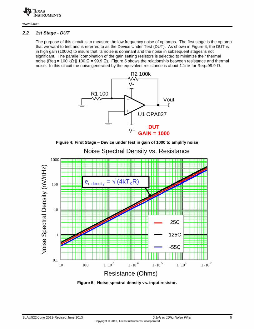
2.2 1st Stage - DUT

The purpose of this circuit is to measure the low frequency noise of op amps. The first stage is the op amp that we want to test and is referred to as the Device Under Test (DUT). As shown in Figure 4, the DUT is in high gain (1000x) to insure that its noise is dominant and the noise in subsequent stages is not significant. The parallel combination of the gain setting resistors is selected to minimize their thermal noise (Req = 100 kΩ || 100 Ω = 99.9 Ω). Figure 5 shows the relationship between resistance and thermal noise. In this circuit the noise generated by the equivalent resistance is about 1.1nV for Req=99.9 Ω.

V-

V+

VoutR1 100

R2 100k

-

+U1 OPA827

DUT

GAIN = 1000

Figure 4: First Stage – Device under test in gain of 1000 to amplify noise

Noise Spectral Density vs. Resistance

Resistance (Ohms)

No

ise

Sp

ectr

al D

en

sity (

nV

/rtH

z)

10 100 1 103

1 104

1 105

1 106

1 107

0.1

1

10

100

1 103

468.916

0.347

4 1.38065 1023

25 273.15( ) X

10

9

4 1.38065 1023

125 273.15( ) X

10

9

4 1.38065 1023

55 273.15( ) X

10

9

10710 X

1000

10 100 1 103

1 104

1 105

1 106

1 107

0.1

1

10

100

1 103

468.916

0.347

4 1.380651023

25 273.15( ) X

10

9

4 1.380651023

125 273.15( ) X

10

9

4 1.380651023

55 273.15( ) X

10

9

10710 X

25C

125C

-55C

en density = √ (4kTKR)

Figure 5: Noise spectral density vs. input resistor.

www.ti.com


The first stage uses DIP sockets to allow easy interchangeability of the DUT. The first stage has four different sockets that are configured for the DIP adaptor card for common packages (i.e. SOT, SO8, SC70, and DUAL-SO8). The PCB silk screen below the dip socket shows the pin configuration for each socket. Figure 6 shows the PCB with a DIP adaptor installed in socket U2. The jumper JMP2 is used to select the output of U2. Figure 7 shows the DIP adaptor card. The gerber files for the DIP adaptor cards are included in the TI-Design folder. Also, all the common DIP adaptor cards are included in the DIP-ADAPTOR-EVM.

DIP Sockets allow the installation of different types of amplifiers. The devices are soldered to DIP adaptor cards.

Jumpers allow the selection of the different sockets.

Figure 6: First stage uses socketed DIP adaptor cards and jumper selection

Figure 7: DIP adaptor board

www.ti.com


Figure 8 shows how the different package configurations in the first stage are jumper selected. It is important that the jumper is connected to only one output at a time to prevent connecting two op amp outputs together.

V-

V+

To

Second

stage

100

100k

-

+SOT-to-DIP

6

3

18

2

V-

V+

100

100k

-

+SO8-to-DIP

2

3

67

4

V-

V+

100

100k

-

+SC70-to-DIP

3

1

68

2

Jumper

selects SOT

Figure 8: First stage uses jumpers to select different package types

www.ti.com


2.3 2ND Stage 0.1Hz HPF

The second stage is a 0.1Hz high pass filter in a gain of 10 (Figure 9). A Texas Instruments software tool called Filter-pro™ can be used to design the filters in this design. The filter was selected to be a second order Butterworth, Sallen-Key, high pass filter. The Butterworth frequency response was selected to be maximally flat. The Sallen-Key topology is used because it produces more reasonable component values; i.e. the capacitors and resistors are in the range available for low cost precision components.

Figure 9: Second Stage – 0.1Hz, 2nd order High Pass Filter, Gain = 10

V+

R7 2M

R1

3 6

34

k

R1

6 1

kR17 9.09k

C11 1u C12 1u

Vout

R8 2M

-

+

U4 OPA827

V-

0.1Hz HPF

2nd

order

G = 10

Vin

To

3rd

stage

www.ti.com


2.4 3RD Stage 10Hz LPF

The third stage is a 10Hz low pass filter in a gain of 10 (Figure 9). The filter was selected to be a second order Butterworth Multiple-Feedback high pass filter. The Butterworth frequency response was selected to be maximally flat. The Multiple-Feedback topology is used because it produces more reasonable component values; i.e. the capacitors and resistors are in the range available for low cost precision components.

Figure 10: Third Stage – 10Hz, 2nd order Low Pass Filter, Gain = 10

V-

V+

R3 1.6M

R9 162k R10 210k

C1

5 1

00

n

C5 7.5n

-

+

10Hz LPF

2nd

order

G = 10

Input

From

2nd

stage

To 4th

stage

www.ti.com


2.5 4th Stage 10Hz LPF

The fourth stage is a 10Hz low pass filter in a gain of 1 (Figure 11). It is similar to the third stage but with a gain of 1. The objective of the third and fourth stage is to create a 4

th order low pass filter. The filter was

selected to be a second order, Butterworth, Multiple-Feedback, high pass filter. The Butterworth frequency response was selected to be maximally flat. The Multiple-Feedback topology is used because it produces more reasonable component values; i.e. the capacitors and resistors are in the range available for low cost precision components.

Figure 11: Fourth Stage – 10Hz, 2nd order Low Pass Filter, Gain = 1

3 Component Selection

3.1 Op Amp Selection

The op amps used in the three stage filter were selected to minimize noise, bias current, and offset drift. The goal is to insure that the filter does not add any noise or drift to the DUT. The reason for using a low drift amplifier is that offset drift and bias current drift can easily be mistaken as noise in the 0.1Hz to 10Hz range. Also note that the impedances involved in the filter are large (i.e. greater then 100k) so low bias current in needed to avoid large offsets and drifts. Because the DUT is in high gain it not really critical that the amplifiers are ultra high precision; nevertheless, it is recommended using a high precision op amp in case lower DUT gain is used. The OPA827 was used in the filter stages for this design.

3.2 Passive Component Selection

It is important for this circuit to have good gain accuracy and accurate cutoff frequencies. The accuracy of the cutoff frequencies is determined by tolerance of the resistors and capacitors in the filters. In general, the tolerance of the capacitors will be the limiting factor. The COG / NPO type chip capacitors have the best accuracy (1% to 5%). These types of capacitors also have the best temperature and voltage coefficients. Unfortunately, these capacitors are only available for smaller capacitance ranges (i.e. C < 0.47uF). As an alternative, X7R capacitors with a high voltage rating (i.e. 50V or greater) and a low tolerance (i.e. 5% or better) can be used where large capacitors are required. Note that capacitors with a larger voltage rating will have a smaller voltage coefficient. The resistors are selected with 1% tolerance or better to minimize gain error.

V-

V+

Vout

R6 825k

R11 825k R12 412k

C1

7 1

00

n

C6 7.5n

-

+U2 OPA827

From

3rd

stage

10Hz LPF

2nd

order

G = 1

Output to

scope

www.ti.com


4 Simulation

The TINA-TI™ schematic shown in Figure 12 includes the circuit values obtained in the design process.

V-

V-V-

V+

V+

V+

V+ V-

R7 2M

R13 6

34k

R16 1

k

R17 9.09k

C11 1u C12 1u

R3 1.6M

R9 162k R10 210k

C15 1

00n

C5 7.5n

Vout

R6 825k

R11 825k R12 412k

C17 1

00n

C6 7.5n

R8 2M+

VG1

R1 100

R2 100k

-

++3

2

7

4

6

U1 OPA827

-

++3

2

7

4

6

U6 OPA827

-

++3

2

7

4

6

U7 OPA827

-

++3

2

7

4

6

U5 OPA827

Figure 12: TINA-TI™ Spice Schematic

www.ti.com


4.1 AC Transfer Function

The simulated dc transfer function of the filter (stages 2, 3, and 4) are shown Figure 13. The results of a Monte-Carlo analysis are shown in Figure 14. The Monte-Carlo analysis uses the resistor and capacitor tolerance to do a statistical analysis that shows the expected variation of the filters transfer function. Table 2 summarizes the results of the Monte-Carlo analysis and compares it to measured results.

Figure 13: Gain vs. Freq for the filter only (Max Gain = 40dB, or 100x)

Figure 14: Monte Carlo Analysis of frequency response

40db/decade

20db/decade

T

Frequency (Hz)

10m 100m 1 10 100

Ga

in (

dB

)

-40.00

-20.00

0.00

20.00

40.00

fL = 0.1Hz fH = 10Hz

T

Frequency (Hz)

10m 100m 1 10 100

Ga

in (

V/V

)

1.00m

10.00m

100.00m

1.00

10.00

100.00

1.00k

T

Frequency (Hz)

10m 100m 1

Ga

in (

dB

)

10.00

100.00

1.00k

www.ti.com


Table 2: Simulated results including statistical variation

Ideal

Nominal

simulation



Measured

Amplitude at 0.1Hz 70.07 70.98 59.56 77.05 67.9

Amplitude at 10Hz 70.07 70.06 61.56 76.57 67.5

Amplitude at 1Hz 100 99.68 96 100.68 98.75

4.2 Simulated Noise results

Figure 15 shows the total integrated noise for the circuit with OPA827 being used as the DUT. This result is the equivalent RMS output noise. To get an estimate of the peak-to-peak noise, multiply this estimate by 6 (see Equation (1)). Figure 16 and Table 3 show the expected variation using the Monte Carlo analysis. The Monte Carlo Analysis will take into account all the variability of the capacitor and resistors tolerance.

Figure 15: Total Noise where OPA827 is the filter amplifier and the DUT

(1)

T

Frequency (Hz)

10m 100m 1 10 100

To

tal n

ois

e (

V)

0.00

2.03m

4.05m

www.ti.com


T

3.8mV rms

4.31mV rms

Frequency (Hz)

10m 100m 1 10 100

To

tal n

ois

e (

V)

0.00

1.00m

2.00m

3.00m

4.00m

5.00m

3.8mV rms

4.31mV rms

Figure 16: Total noise variability using Monte Carlo Analysis for OPA827

Table 3: Summary of total noise variability using Monte Carlo Analysis

Data sheet Nominal

simulated

Simulated Monte Carlo

Low

Simulated Monte Carlo

High

Measured

OPA827

0.1Hz to 10Hz

250nVpp

41.7nV rms

243nVpp 40.5nV rms

228nVpp

38nV rms

258nVpp

43.1nVpp

250nVpp

41.7nV rms

www.ti.com


5 PCB Design

The PCB schematic and Bill of Materials can be found in Section 8.

5.1 PCB Layout

The general guidelines for precision PCB layout were used on this design. For example, trace lengths are kept to minimum length especially input signals.

Figure 17: PCB Layout (Top on Left, Bottom on Right)

www.ti.com


6 Verification & Measured Performance

6.1 General precautions used in measuring 0.1Hz to 10Hz noise

Figure 18 shows the test setup to confirm the operation of the 0.1Hz to 10Hz filter. The idea behind this setup is to sweep the frequency of the input and measure the gain vs. frequency response for the filter. This setup is only for initial test and characterization of the board. After initial test, the setup shown in Figure 19 will be used to measure the 0.1Hz to 10Hz noise.

It is important to use a shielded environment to get the best results from this test. Figure 20 shows the one possible option for a shielded environment. This is a steel paint can with BNC and banana connections drilled through the top. This shield is effective at shielding the noise filter from 60Hz and other noise pickup. It also minimizes temperature shifts by protecting the board from air turbulence. It is important that the entire shield is grounded, and minimal air gaps (slot antennas). If a paint can is used, make sure that the lid and can make a good seal. It may be necessary to sand the rim in the lid of the paint can to insure that the lid and can make good electrical contact.

Signal generator50mVpk

0.01Hz to 100Hz

Digitizing Oscilloscope

Low noise Linear Power Supply+/-15V+/- 0.01V

Coax

Coax

Banana

Shielded Test environment

0.1 to 10HzNoise Filter

Figure 18: Test setup for V-to-I board

www.ti.com


Digitizing Oscilloscope

Low noise Linear Power Supply+/-15V+/- 0.01V

Coax

Banana

Shielded Test environment

0.1 to 10HzNoise Filter

Figure 19: Setup for testing 0.1Hz to 10Hz noise

Figure 20: Shielded environment used to measure noise

www.ti.com


6.2 Transfer Function

Data was collected by sweeping the frequency of VIN from 0.03Hz to 50Hz while measuring output response. This measurement is made for the filter only (Vin to J5 and Vout to J4 on the PCB). Figure 21 displays the measured results in Volts-per-Volt . The errors measured at specific frequency are summarized in Table 4.

Figure 21: Measured Filter Response

Table 4: Summary of measured errors at key frequencies

Ideal Nominal



Measured

Amplitude at 0.1Hz (V/V) 70.07 70.98 59.56 77.05 67.9

Amplitude at 10Hz (V/V) 70.07 70.06 61.56 76.57 67.5

Amplitude at 1Hz (V/V) 100 99.68 96 100.68 98.75

www.ti.com


6.3 Measured scope output

The goal of this circuit is to produce the 0.1Hz to 10Hz oscilloscope noise measurements that are given in data sheets. Figure 22 shows the 0.1Hz to 10Hz noise measurement for the OPA277 as well as its spectral density. The spectral density curve can be used with a hand calculation to confirm that the 0.1Hz to 10Hz measurement is correct. Equations (2) and (3) show the calculation for the expected noise for an OPA277 with the 0.1Hz to 10Hz filter. Equations (1) normalizes the flicker noise to 1Hz and equation (3) integrates the noise from 0.1Hz to 10Hz. Further details on the derivation and usage of these equations are given in reference 1. In this case the measured result is lower than expected (En-meas = 150nV, En-calc = 218nV). Equation (4) shows how the scope reading is divided by the gain to obtain the noise RTI.

Figure 22: Scope noise output and voltage noise spectral density for OPA277

(2)

(3)

(4)

OPA277, 50nV/divEn = 150nVpp

50nV/rtHzAt 0.1Hz

0.1Hz to 10HzNoise measured by Scope

www.ti.com


Figure 23 is a second example showing how the measured filter output can be predicted using the spectral density curve and hand calculations. Equations (5), and (6) show the hand calculation of the filter output noise. Figure 24 shows two additional measured results but does not show the hand calculations. Equation (7) shows how the scope reading is divided by the gain to obtain the noise RTI.

Figure 23: Scope noise output and voltage noise spectral density for OPA1652

(5)

(6)

(7)


OPA170, 1uV/divEn = 2.4uVpp

Figure 24: Measured 0.1Hz to 10Hz noise for OPA827 and OPA170


35nV/rtHzAt 10Hz

0.1Hz to 10HzNoise measured by Scope

www.ti.com


6.4 Measured Result Summary

Table 5 summarizes the measured results for the four example amplifiers tested using the filter board. The data sheet typical specification for 0.1Hz to 10Hz noise is given for comparison. In general the circuit performs well.

Table 5: Data sheet specifications vs. measured results for five examples.

Op amp Data Sheet Noise spec

Measured

OPA827 250nVpp 250nVpp

OPA277 220nVpp 150nVpp

OPA170 2.0uVpp 2.4uVpp

OPA1652 1.5uVpp 1.5uVpp

www.ti.com


7 Modifications

7.1 Selecting different amplifiers

The example shown in this design used the OPA827 in the filter stages. Other amplifiers that would be suitable for the filter are given in Table 6. Any amplifier can be tested as the DUT. The same fixture can be used for 5V amplifiers (e.g. OPA333). In the case of these type amplifiers use +/-2.5V supplies to avoid common mode limitations.

Table 6: Brief Comparison of Amplifiers

Amplifier Max Supply Voltage (V)

Max Offset Voltage (uV)

Max Offset Drift (uV/C)

Bandwidth (MHz) Bias Current

(pA)

OPA827 36 150 2 22 10

OPA277 36 20 0.15 1 2800

OPA188 36 25 0.085 1 1400

OPA333 5.5 10 0.05 0.35 200

OPA335 5.5 5 0.05 2 200

7.2 Different DUT gain

The gain of the DUT was set to 1,000 to amplify noise so that it is measureable and also to insure that the first DUT is the dominant noise source. In some cases it may be useful to change the gain of the first stage.

8 About the Author

Arthur Kay is an applications engineering manager at TI where he specializes in the support of amplifiers, references, and mixed signal devices. Arthur focuses a good deal on industrial applications such as bridge sensor signal conditioning. Arthur has published a book and an article series on amplifier noise. Before working in applications engineering, he was a semiconductor test engineer for Burr-Brown and Northrop Grumman Corp. Arthur received his MSEE from Georgia Institute of Technology (1993), and BSEE from Cleveland State University (1992).

9 Acknowledgements & References

[1] Kay, A., Operational Amplifier Noise, Newnes, 2012, Chapter 5

[2] DIP Adapter EVM, Tool, Texas Instruments, http://www.ti.com/tool/dip-adapter-evm

[2] Filter Pro, Tool, Texas Instruments, http://www.ti.com/tool/filterpro

http://www.ti.com/tool/dip-adapter-evm

http://www.ti.com/tool/filterpro

www.ti.com


Appendix A. Appendix

A.1 Electrical Schematic and Bill of Materials

The electrical schematic and bill of materials for this design are shown in Figure A-1 and Figure A-2, respectively.

Figure A-1: Electrical Schematic

www.ti.com


A.2 Bill of Materials

Item Qty Value Designator Description Manufacturer Manufacturer Part No. Supplier Part No.

1 14 0.1uF

C1, C4, C7, C8, C9, C10, C13,

C14, C16, C18, C19, C20,

C21, C22 CAP, CERM, 0.1uF, 50V, +/-5%, X7R, 0805 AVX 08055C104JAT2A 478-3352-1-ND

2 2 4.7uF C2, C3

CAP, CERM, 4.7uF, 16V, +/-20%, X7R,

1206 TDK C3216X7R1C475M160AB 445-5994-1-ND

3 2 7.5n C5, C6 CAP CER 7500PF 50V 5% NP0 0805 TDK GRM2195C1H752JA01D 490-1639-1-ND

4 2 1uF C11, C12 CAP, CERM, 1uF, 50V, +/-10%, X7R, 0805 TDK C2012X6S1H105K085AB 445-14501-1-ND

5 2 0.1uF C15, C17 CAP CER 1UF 50V 10% X6S 0805 TDK C2012X6S1H105K085AB 445-14501-1-ND

6 4 H1, H2, H3, H4

Machine Screw, Round, #4-40 x 1/4,

Nylon, Philips panhead B&F Fastener NY PMS 440 0025 PH H542-ND

7 1 Vs+ J1

Standard Banana Jack, Uninsulated,

5.5mm Keystone 575-4 575-4K-ND

8 1 GND J2



9 1 Vs- J3



10 2 J4, J5 CONN BNC JACK R/A 75 OHM PCB TE Connectivity 1-1478032-0 A97560-ND

11 5

JMP1, JMP2, JMP3, JMP4,

JMP5, JMP6, JMP7

CONN HEADER 50POS .100" SGL GOLD

(cut as needed) Samtec Inc TSW-150-07-G-S SAM1029-50-ND

12 5 10 R1, R4, R14, R18, R20 RES 10.0 OHM 1/10W 0.1% 0805 TE Connectivity 1-1614884-7 A103143CT-ND

13 5 10.0k R2, R5, R15, R19, R21 RES 10K OHM 1/8W .1% 0805 SMD Panasonic ERA-6AEB103V P10KDACT-ND

14 1 1.6M R3 RES 1.6M OHM 1/10W 0.1% 0805 TE Connectivity 1-1614959-2 A103800CT-ND

15 2 825k R6, R11 RES 825K OHM 1/8W 0.5% 0805 SMD Panasonic ERA-6AED8253V P825KBNCT-ND

16 2 2.00Meg R7, R8 RES, 2.00Meg ohm, 1%, 0.125W, 0805 Vishay-Dale CRCW08052M00FKEA 541-2.00MCCT-ND

17 1 162k R9 RES 162K OHM 1/8W .1% 0805 SMD Vishay-Dale ERA-6AEB1623V P162KDACT-ND

18 1 210k R10 RES 210K OHM 1/8W .1% 0805 SMD Panasonic ERA-6AEB2103V P210KDACT-ND



21 1 1.00k R16 RES, 1.00k ohm, 1%, 0.125W, 0805 Panasonic ERA-6AEB102V P1.0KDACT-ND

22 1 9.09k R17 RES 9.09K OHM 1/8W .1% 0805 SMD Panasonic ERA-6AEB9091V P9.09KDACT-ND

23 0 R23

Optional for gain set, Do Not Populate

for Gain=1

24 1 0 R22 RES 0.0 OHM 1/8W JUMP 0805 SMD Panasonic ERJ-6GEY0R00V P0.0ACT-ND

25 1 GND TP1 Test Point, TH, Compact, Red Keystone 5124 5005K-ND

26 1 Vs- TP2 Test Point, TH, Compact, Red Keystone 5124 5005K-ND

27 1 Vs+ TP3 Test Point, TH, Compact, Red Keystone 5124 5005K-ND

28 3 U5, U6, U7, U8 IC OPAMP JFET 22MHZ SGL 8VSSOP Texas Inst. OPA827AID 296-24280-1-ND

Figure A-2: Bill of Materials

IMPORTANT NOTICE FOR TI REFERENCE DESIGNS

Texas Instruments Incorporated ("TI") reference designs are solely intended to assist designers (“Buyers”) who are developing systems thatincorporate TI semiconductor products (also referred to herein as “components”). Buyer understands and agrees that Buyer remainsresponsible for using its independent analysis, evaluation and judgment in designing Buyer’s systems and products.

TI reference designs have been created using standard laboratory conditions and engineering practices. TI has not conducted anytesting other than that specifically described in the published documentation for a particular reference design. TI may makecorrections, enhancements, improvements and other changes to its reference designs.

Buyers are authorized to use TI reference designs with the TI component(s) identified in each particular reference design and to modify thereference design in the development of their end products. HOWEVER, NO OTHER LICENSE, EXPRESS OR IMPLIED, BY ESTOPPELOR OTHERWISE TO ANY OTHER TI INTELLECTUAL PROPERTY RIGHT, AND NO LICENSE TO ANY THIRD PARTY TECHNOLOGYOR INTELLECTUAL PROPERTY RIGHT, IS GRANTED HEREIN, including but not limited to any patent right, copyright, mask work right,or other intellectual property right relating to any combination, machine, or process in which TI components or services are used.Information published by TI regarding third-party products or services does not constitute a license to use such products or services, or awarranty or endorsement thereof. Use of such information may require a license from a third party under the patents or other intellectualproperty of the third party, or a license from TI under the patents or other intellectual property of TI.

TI REFERENCE DESIGNS ARE PROVIDED "AS IS". TI MAKES NO WARRANTIES OR REPRESENTATIONS WITH REGARD TO THEREFERENCE DESIGNS OR USE OF THE REFERENCE DESIGNS, EXPRESS, IMPLIED OR STATUTORY, INCLUDING ACCURACY ORCOMPLETENESS. TI DISCLAIMS ANY WARRANTY OF TITLE AND ANY IMPLIED WARRANTIES OF MERCHANTABILITY, FITNESSFOR A PARTICULAR PURPOSE, QUIET ENJOYMENT, QUIET POSSESSION, AND NON-INFRINGEMENT OF ANY THIRD PARTYINTELLECTUAL PROPERTY RIGHTS WITH REGARD TO TI REFERENCE DESIGNS OR USE THEREOF. TI SHALL NOT BE LIABLEFOR AND SHALL NOT DEFEND OR INDEMNIFY BUYERS AGAINST ANY THIRD PARTY INFRINGEMENT CLAIM THAT RELATES TOOR IS BASED ON A COMBINATION OF COMPONENTS PROVIDED IN A TI REFERENCE DESIGN. IN NO EVENT SHALL TI BELIABLE FOR ANY ACTUAL, SPECIAL, INCIDENTAL, CONSEQUENTIAL OR INDIRECT DAMAGES, HOWEVER CAUSED, ON ANYTHEORY OF LIABILITY AND WHETHER OR NOT TI HAS BEEN ADVISED OF THE POSSIBILITY OF SUCH DAMAGES, ARISING INANY WAY OUT OF TI REFERENCE DESIGNS OR BUYER’S USE OF TI REFERENCE DESIGNS.

TI reserves the right to make corrections, enhancements, improvements and other changes to its semiconductor products and services perJESD46, latest issue, and to discontinue any product or service per JESD48, latest issue. Buyers should obtain the latest relevantinformation before placing orders and should verify that such information is current and complete. All semiconductor products are soldsubject to TI’s terms and conditions of sale supplied at the time of order acknowledgment.

TI warrants performance of its components to the specifications applicable at the time of sale, in accordance with the warranty in TI’s termsand conditions of sale of semiconductor products. Testing and other quality control techniques for TI components are used to the extent TIdeems necessary to support this warranty. Except where mandated by applicable law, testing of all parameters of each component is notnecessarily performed.

TI assumes no liability for applications assistance or the design of Buyers’ products. Buyers are responsible for their products andapplications using TI components. To minimize the risks associated with Buyers’ products and applications, Buyers should provideadequate design and operating safeguards.

Reproduction of significant portions of TI information in TI data books, data sheets or reference designs is permissible only if reproduction iswithout alteration and is accompanied by all associated warranties, conditions, limitations, and notices. TI is not responsible or liable forsuch altered documentation. Information of third parties may be subject to additional restrictions.

Buyer acknowledges and agrees that it is solely responsible for compliance with all legal, regulatory and safety-related requirementsconcerning its products, and any use of TI components in its applications, notwithstanding any applications-related information or supportthat may be provided by TI. Buyer represents and agrees that it has all the necessary expertise to create and implement safeguards thatanticipate dangerous failures, monitor failures and their consequences, lessen the likelihood of dangerous failures and take appropriateremedial actions. Buyer will fully indemnify TI and its representatives against any damages arising out of the use of any TI components inBuyer’s safety-critical applications.

In some cases, TI components may be promoted specifically to facilitate safety-related applications. With such components, TI’s goal is tohelp enable customers to design and create their own end-product solutions that meet applicable functional safety standards andrequirements. Nonetheless, such components are subject to these terms.

No TI components are authorized for use in FDA Class III (or similar life-critical medical equipment) unless authorized officers of the partieshave executed an agreement specifically governing such use.

Only those TI components that TI has specifically designated as military grade or “enhanced plastic” are designed and intended for use inmilitary/aerospace applications or environments. Buyer acknowledges and agrees that any military or aerospace use of TI components thathave not been so designated is solely at Buyer's risk, and Buyer is solely responsible for compliance with all legal and regulatoryrequirements in connection with such use.

TI has specifically designated certain components as meeting ISO/TS16949 requirements, mainly for automotive use. In any case of use ofnon-designated products, TI will not be responsible for any failure to meet ISO/TS16949.

Mailing Address: Texas Instruments, Post Office Box 655303, Dallas, Texas 75265Copyright © 2013, Texas Instruments Incorporated

Documents

Arthur Kay TI Precision Designs: Verified Design 0.1Hz to ... · 0.1Hz to 10Hz Noise Filter TI Precision Designs Circuit Description TI Precision Designs are analog solutions created