Embed Size (px)
Citation preview

JSS Journal of Statistical SoftwareMMMMMM YYYY Volume VV Issue II httpwwwjstatsoftorg
Parameter Estimation of ARMA Models with
GARCHAPARCH Errors
An R and SPlus Software Implementation
Diethelm Wurtz1 Yohan Chalabi2 Ladislav Luksan3
12Institute for Theoretical PhysicsSwiss Federal Institute of Technology Zurich3Academy of Sciences of the Czech Republic
Institute of Computer Science Praha
Abstract
We report on concepts and methods to implement the family of ARMA models withGARCHAPARCH errors introduced by Ding Granger and Engle The software imple-mentation is written in S and optimization of the constrained log-likelihood function isachieved with the help of a SQP solver The implementation is tested with BollerslevrsquosGARCH(11) model applied to the DEMGBP foreign exchange rate data set given byBollerslev and Ghysels The results are compared with the benchmark implementationof Fiorentini Calzolari and Panattoni In addition the MA(1)-APARCH(11) model forthe SP500 stock market index analyzed by Ding Granger and Engle is reestimated andcompared with results obtained from the OxGRCH and SPlusFinmetrics softwarepackages The software is part of the Rmetrics open source project for computationalfinance and financial engineering Implementations are available for both software envi-ronments R and SPlus
Keywords Time Series Analysis Heteroskedasticity ARCH GARCH APARCH constrainedmaximum log-likelihood SQP solver R Rmetrics SPlus Finmetrics Ox GRCH
1 Introduction
GARCH Generalized Autoregressive Conditional Heteroskedastic models have become im-portant in the analysis of time series data particularly in financial applications when the goalis to analyze and forecast volatility For this purpose we describe functions for simulatingestimating and forecasting various univariate GARCH-type time series models in the condi-tional variance and an ARMA specification in the conditional mean We present a numerical
2 An R and SPlus Software Implementation
implementation of the maximum log-likelihood approach under different assumptions Nor-mal Student-t GED errors or their skewed versions The parameter estimates are checkedby several diagnostic analysis tools including graphical features and hypothesis tests Func-tions to compute n-step ahead forecasts of both the conditional mean and variance are alsoavailable
The number of GARCH models is immense but the most influential models were the firstBeside the standard ARCH model introduced by Engle [1982] and the GARCH model in-troduced by Bollerslev [1986] we consider also the more general class of asymmetric powerARCH models named APARCH introduced by Ding Granger and Engle [1993] APARCHmodels include as special cases the TS-GARCH model of Taylor [1986] and Schwert [1989]the GJR-GARCH model of Glosten Jaganathan and Runkle [1993] the T-ARCH model ofZakoian [1993] the N-ARCH model of Higgins and Bera [1992] and the Log-ARCH model ofGeweke [1986] and Pentula [1986]
Coupled with these models was a sophisticated analysis of the stochastic process of data gen-erated by the underlying process as well as estimators for the unknown model parametersTheorems for the autocorrelations moments and stationarity and ergodicity of GARCH pro-cesses have been developed for many of the important cases There exist a collection of reviewarticles by Bollerslev Chou and Kroner [1992] Bera and Higgins [1993] Bollerslev Engle andNelson [1994] Engle [2001] Engle and Patton [2001] and Li Ling and McAleer [2002] thatgive a good overview of the scope of the research
2 Mean and Variance Equation
We describe the mean equation of an univariate time series xt by the process
xt = E(xt|Ωtminus1) + εt (1)
where E(middot|middot) denotes the conditional expectation operator Ωtminus1 the information set at time tminus1 and εt the innovations or residuals of the time series εt describes uncorrelated disturbanceswith zero mean and plays the role of the unpredictable part of the time series In the followingwe model the mean equation as an ARMA process and the innovations are generated from aGARCH or APARCH process
ARMA Mean Equation The ARMA(mn) process of autoregressive order m and movingaverage order n can be described as
xt = micro +msum
i=1
aixtminusi +nsum
j=1
bjεtminusj + εt
= micro + a(B)xt + b(B)εt (2)
with mean micro autoregressive coefficients ai and moving average coefficients bi Note thatthe model can be expressed in a quite comprehensive form using the backshift operator Bdefined by Bxt = xtminus1 The functions a(B) and b(B) are polynomials of degree m and nrespectively in the backward shift operator B If n = 0 we have a pure autoregressive processand if on the other hand m = 0 we have a pure moving average process The ARMA time
Journal of Statistical Software 3
series is stationary when the series a(B) which is the generating function of the coefficientsai converges for |B| lt 1 that is on or within the unit circle
GARCH Variance Equation The mean equation cannot take into account for heteroskedas-tic effects of the time series process typically observed in form of fat tails as clustering ofvolatilities and the leverage effect In this context Engle [1982] introduced the Autoregres-sive Conditional Heteroskedastic model named ARCH later generalized by Bollerslev [1986]named GARCH The εt terms in the ARMA mean equation (2) are the innovations of thetime series process Engle [1982] defined them as an autoregressive conditional heteroscedasticprocess where all εt are of the form
εt = zt σt (3)
where zt is an iid process with zero mean and unit variance Although εt is serially uncor-related by definition its conditional variance equals σ2
t and therefore may change over timeAll the GARCH models we consider in the following differ only in their functional form forthe conditional variance
The variance equation of the GARCH(pq) model can be expressed as
εt = ztσt
zt sim Dϑ(0 1)
σ2t = ω +
psumi=1
αiε2tminusi +
qsumj=1
βjσ2tminusj
= ω + α(B)ε2tminus1 + β(B)σ2
tminus1 (4)
where Dϑ(0 1) is the probability density function of the innovations or residuals with zeromean and unit variance Optionally ϑ are additional distributional parameters to describethe skew and the shape of the distribution If all the coefficients β are zero the GARCHmodel is reduced to the ARCH model Like for ARMA models a GARCH specification oftenleads to a more parsimonious representation of the temporal dependencies and thus providesa similar added flexibility over the linear ARCH model when parameterizing the conditionalvariance Bolerslev [1986] has shown that the GARCH(pq) process is wide-sense stationarywith E(εt) = 0 var(εt) = ω(1 minus α(1) minus β(1)) and cov(εt εs) = 0 for t 6= s if and only ifα(1) + β(1) lt 1
The variance equation of the APARCH(pq) model can be written as
εt = ztσt
zt sim Dϑ(0 1)
σδt = ω +
psumi=1
αi(|εtminusi| minus γiεtminusi)δ +qsum
j=1
βjσδtminusj (5)
where δ gt 0 and minus1 lt γi lt 1 This model has been introduced by Ding Granger and Engle[1993] It adds the flexibility of a varying exponent with an asymmetry coefficient to take the
4 An R and SPlus Software Implementation
leverage effect into account A stationary solution exists if ω gt 0 and Σiαiκi + Σjβj lt 1where κi = E(|z|+ γiz)δ Note that if γ 6= 0 andor δ 6= 2 the κi depend on the assumptionsmade on the innovation process The family of APARCH models includes the ARCH andGARCH models and five other ARCH extensions as special cases
bull ARCH Model of Engle when δ = 2 γi = 0 and βj = 0
bull GARCH Model of Bollerslev when δ = 2 and γi = 0
bull TS-GARCH Model of Taylor and Schwert when δ = 1 and γi = 0
bull GJR-GARCH Model of Glosten Jagannathan and Runkle when δ = 2
bull T-ARCH Model of Zakoian when δ = 1
bull N-ARCH Model of Higgens and Bera when γi = 0 and βj = 0
bull Log-ARCH Model of Geweke and Pentula when δ rarr 0
3 The Standard GARCH(11) Model
Code Snippet 1 shows how to write a basic S function named garch11Fit() to estimatethe parameters for Bollerslevrsquos GARCH(11) model As the benchmark data set we use thedaily DEMGBP foreign exchange rates as supplied by Bollerslev and Ghysels [1996] and theresults obtained by Fiorentini Calzolar and Panattoni [1996] based on the optimization of thelog-likelihood function using analytic expressions for the gradient and Hessian matrix Thissetting is well accepted as the benchmark for GARCH(11) models The function estimatesthe parameters micro ω α β in a sequence of several major steps (1) the initialization of thetime series (2) the initialization of the model parameters (3) the settings for the conditionaldistribution function (4) the composition of the log-likelihood function (5) the estimationof the model parameters and 6) the summary of the optimization results
Given the model for the conditional mean and variance and an observed univariate returnseries we can use the maximum log-likelihood estimation approach to fit the parameters forthe specified model of the return series The procedure infers the process innovations orresiduals by inverse filtering Note that this filtering transforms the observed process εt intoan uncorrelated white noise process zt The log-likelihood function then uses the inferredinnovations zt to infer the corresponding conditional variances σt
2 via recursive substitutioninto the model-dependent conditional variance equations Finally the procedure uses theinferred innovations and conditional variances to evaluate the appropriate log-likelihood ob-jective function The MLE concept interprets the density as a function of the parameter setconditional on a set of sample outcomes The Normal distribution is the standard distributionwhen estimating and forecasting GARCH models Using εt = ztσt the log-likelihood functionof the Normal distribution is given by
LN (θ) = lnprod
t
1radic(2πσ2
t )eminus ε2t
2σ2t = ln
prodt
1radic(2πσ2
t )eminus
z2t2 (6)
= minus12
sumt
[log(2π) + log(σ2t ) + z2
t ]
Journal of Statistical Software 5
or in general
LN (θ) = lnprod
t
Dϑ(xt E(xt|Ωtminus1) σt) (7)
where Dϑ is the conditional distribution function The second argument of Dϑ denotesthe mean and the third argument the standard deviation The full set of parametersθ includes the parameters from the mean equation (micro a1m b1n) from the variance equa-tion (ω α1p γ1p β1q δ) and the distributional parameters (ϑ) in the case of a non-normaldistribution function For Bollerslevrsquos GARCH(11) model the parameter set reduces toθ = micro ω α1 β1 In the following we will suppress the index on the parameters α andβ if we consider the GARCH(11) modelThe parameters θ which fit the model best are obtained by minimizing the ldquonegativerdquo log-likelihood function Some of the values of the parameter set θ are constrained to a finite orsemi-finite range Note that ω gt 0 has to be constrained on positive values and that α andβ have to be constrained in a finite interval [0 1) This requires a solver for constrainednumerical optimization problems R offers the solvers nlminb() and optim(method=L-BFGS-B) for constrained optimization the first is also part of SPlus These are R interfacesto underlying Fortran routines from the PORT Mathematical Subroutine Library LucentTechnologies [1997] and to TOMS Algorithm 778 ACM [1997] respectively In additionwe have implemented a sequential quadratic programming algorithm sqp Lucsan [1976]which is more efficient compared to the other two solvers And additionally everythingis implemented in Fortran the solver the objective function gradient vector and HessianmatrixThe optimizer require a vector of initial parameters for the mean micro as well as for the GARCHcoefficients ω α and β The initial value for the mean is estimated from the mean micro of thetime series observations x For the GARCH(11) model we initialize α = 01 and β = 08by typical values of financial time series and ω by the variance of the series adjusted by thepersistence ω = Var(x) lowast (1minus αminus β) Further arguments to the GARCH fitting function arethe upper and lower box bounds and optional control parameters
31 How to fit Bollerslevrsquos GARCH(11) Model
In what follows we explicitly demonstrate how the parameter estimation for the GARCH(11)model with normal innovations can be implemented in S The argument list of the fittingfunction garch11Fit(x) requires only the time series the rest will be done automaticallystep by step
bull Step 1 - Series Initialization We save the time series x globally to have the valuesavailable in later function calls without parsing the series through the argument list
bull Step 2 - Parameter Initialization In the second step we initialize the set of modelparameters θ params and the corresponding upper and lower bounds In the examplewe use bounds lowerBounds and upperBounds which are wide enough to serve almostevery economic and financial GARCH(11) model and define model parameters whichtake typical values
bull Step 3 - Conditional Distribution For the conditional distribution we use the Normaldistribution dnorm()
6 An R and SPlus Software Implementation
garch11Fit = function(x)
Step 1 Initialize Time Series Globally
x ltlt- x
Step 2 Initialize Model Parameters and Bounds
Mean = mean(x) Var = var(x) S = 1e-6
params = c(mu = Mean omega = 01Var alpha = 01 beta = 08)
lowerBounds = c(mu = -10abs(Mean) omega = S^2 alpha = S beta = S)
upperBounds = c(mu = 10abs(Mean) omega = 100Var alpha = 1-S beta = 1-S)
Step 3 Set Conditional Distribution Function
garchDist = function(z hh) dnorm(x = zhh)hh
Step 4 Compose log-Likelihood Function
garchLLH = function(parm)
mu = parm[1] omega = parm[2] alpha = parm[3] beta = parm[4]
z = (x-mu) Mean = mean(z^2)
Use Filter Representation
e = omega + alpha c(Mean z[-length(x)]^2)
h = filter(e beta r init = Mean)
hh = sqrt(abs(h))
llh = -sum(log(garchDist(z hh)))
llh
print(garchLLH(params))
Step 5 Estimate Parameters and Compute Numerically Hessian
fit = nlminb(start = params objective = garchLLH
lower = lowerBounds upper = upperBounds control = list(trace=3))
epsilon = 00001 fit$par
Hessian = matrix(0 ncol = 4 nrow = 4)
for (i in 14)
for (j in 14)
x1 = x2 = x3 = x4 = fit$par
x1[i] = x1[i] + epsilon[i] x1[j] = x1[j] + epsilon[j]
x2[i] = x2[i] + epsilon[i] x2[j] = x2[j] - epsilon[j]
x3[i] = x3[i] - epsilon[i] x3[j] = x3[j] + epsilon[j]
x4[i] = x4[i] - epsilon[i] x4[j] = x4[j] - epsilon[j]
Hessian[i j] = (garchLLH(x1)-garchLLH(x2)-garchLLH(x3)+garchLLH(x4))
(4epsilon[i]epsilon[j])
Step 6 Create and Print Summary Report
secoef = sqrt(diag(solve(Hessian)))
tval = fit$parsecoef
matcoef = cbind(fit$par secoef tval 2(1-pnorm(abs(tval))))
dimnames(matcoef) = list(names(tval) c( Estimate
Std Error t value Pr(gt|t|)))
cat(nCoefficient(s)n)
printCoefmat(matcoef digits = 6 signifstars = TRUE)
Code Snippet 1 Example script which shows the six major steps to estimate the parameters
of a GARCH(11) time series model The same steps are implemented in the ldquofull versionrdquo of
garchFit() which allows the parameter estimation of general ARMA(mn)-APARCH(pq) with
several types of conditional distribution functions
Journal of Statistical Software 7
bull Step 4 - Log-Likelihood Function The function garchLLH() computes theldquonegativerdquolog-likelihood for the GARCH(11) model We use a fast and efficient filter representationfor the variance equation such that no execution time limiting for loop will becomenecessary
bull Step 5 - Parameter Estimation For the GARCH(11) model optimization of the log-likelihood function we use the constrained solver nlminb() which is available in Rand SPlus To compute standard errors and t-values we evaluate the Hessian matrixnumerically
bull Step 6 - Summary Report The results for the estimated parameters together withstandard errors and t-values are summarized and printed
32 Case Study The DEMGBP Benchmark
Through the complexity of the GARCH models it is evident that different software imple-mentations have different functionalities drawbacks and features and may lead to differencesin the numerical results McCullough and Renfro [1999] Brooks Burke and Persand [2001]and Laurent and Peters [2003] compared the results of several software packages These in-vestigations demonstrate that there could be major differences between estimated GARCHparameters from different software packages Here we use for comparisons the well acceptedbenchmark suggested by Fiorentini Calzolari and Panattoni [1996] to test our implementa-tionFor the time series data we take the DEMGBP daily exchange rates as published by Bollerslevand Ghysels [1996] The series contains a total of 1975 daily observations sampled during theperiod from January 2 1984 to December 31 1991 This benchmark was also used byMcCullough and Renfro [1999] and by Brooks Burke and Persand [2001] in their analysisof several GARCH software packages Figure 1 shows some stylized facts of the log-returnsof the daily DEMGBP FX rates The distribution is leptokurtic and skewed to negativevalues The log-returns have a mean value of micro = minus000016 ie almost zero a skewness ofς = minus025 and an excess kurtosis of κ = 362 The histogram of the density and the quantile-quantile plot graphically display this behavior Furthermore the autocorrelation function ofthe absolute values of the returns which measures volatility decay slowlyWe use the GARCH(11) model to fit the parameters of the time series using the functiongarch11Fit() and compare these results with the benchmark computations of FiorentiniCalzolari and Panattoni and with results obtained from other statistical software packages
Code Snippet 2 GARCH(11) Benchmark for the DEMGBP Exchange Rates
gt data(dem2gbp)
gt garch11Fit(x = dem2gbp[ 1])
Coefficient(s)
Estimate Std Error t value Pr(gt|t|)
mu -000619040 000846211 -073154 046444724
omega 001076140 000285270 377236 000016171
alpha 015313411 002652273 577369 77552e-09
beta 080597365 003355251 2402126 lt 222e-16
---
Signif codes 0 rsquorsquo 0001 rsquorsquo 001 rsquorsquo 005 rsquorsquo 01 rsquo rsquo 1
8 An R and SPlus Software Implementation
index
log
Ret
urn
0 500 1000 1500 2000
minus0
02minus
001
000
001
002
003
DEMGBP FX Rate Histogram of demgbp
demgbp
Den
sity
minus002 minus001 000 001 002
020
4060
8010
012
0
minus3 minus2 minus1 0 1 2 3
minus0
02minus
001
000
001
002
003
Normal QminusQ Plot
Normal Quantiles
Em
piric
al Q
uant
iles
0 5 10 15 20 25 30
00
02
04
06
08
10
Lag
AC
F
Series abs(demgbp)
Figure 1 Returns their distribution the quantile-quantile plot and the autocorrelation function ofthe volatility for the DEMGBP benchmark data set
The estimated model parameters are to more than four digests exactly the same numbers asthe FCP benchmark Note we used numerically computed derivatives whereas the benchmarkused analytically calculated derivatives The observation that it is not really necessary tocompute the derivatives analytically was already made by Doornik [2000] and Laurent andPeters [2001]
Rmetrics FCP Finmetrics GARCH Shazam TSP
μ -0006190 -0006190 -0006194 -0006183 -0006194 -0006190ω 001076 001076 001076 001076 001076 001076α 01531 01531 01540 01531 01531 01531β 08060 08060 08048 08059 08060 08060
Rmetrics FCP Benchmark GARCH OxEstimate StdErrors Estimate StdErrors Estimate StdErrorsdErrors
μ 000619040 00846211 -000619041 00846212 -0006184 0008462 ω 00107614 00285270 00107614 00285271 0010760 0002851 α 0153134 00265227 0153134 00265228 0153407 0026569 β 0805974 00335525 0805974 00335527 0805879 0033542
Rmetrics FCP Benchmark OxGarch SplusFinmetricsEstimate StdError t Value Estimate StdError t Value Estimate StdError t Value Estimate StdError t Value
μ -00061904 00084621 -0732 -00061904 00084621 -0732 -0006184 0008462 -0731 -0006053 000847 -0715ω 0010761 00028527 377 0010761 00028527 377 0010761 00028506 377 0010896 00029103 374α 015313 0026523 577 015313 0026523 577 015341 0026569 577 015421 0026830 575β 080597 0033553 240 080597 0033553 240 080588 0033542 240 080445 0034037 236
Table 1 Comparison of the results of the GARCH(11) parameter estimation for the DEMGBPbenchmark data set obtained from several software packages The first two columns show the results from theGARCH(11) example program the second group from the FCP benchmark results the third group from OxrsquoGRCH and the last group from SPlusrsquo Finmetrics The left hand numbers are the parameter estimates andthe right hand number the standard errors computed from the Hessian matrix
Journal of Statistical Software 9
4 Alternative Conditional Distributions
Different types of conditional distribution functions D are discussed in literature These arethe Normal distribution which we used in the previous section the standardized Student-tdistribution and the generalized error distribution and their skewed versions Since only thesymmetric Normal distribution of these functions is implemented in Rrsquos base environmentand also in most of the other statistical software packages we discuss the implementation ofthe other distributions in some more detail
The default choice for the distribution D of the innovations zt of a GARCH process is theStandardized Normal Probability Function
f(z) =1radic2π
eminusz2
2 (8)
The probability function or density is named standardized marked by a star because f(z)has zero mean and unit variance This can easily be verified computing the moments
micror =
int infin
minusinfinzrf(z)dz (9)
Note that micro0 equiv 1 and σ
1 equiv 1 are the normalization conditions that micro1 defines the mean
micro equiv 0 and micro2 the variance σ2 equiv 1
An arbitrary Normal distribution located around a mean value micro and scaled by the standarddeviation σ can be obtained by introducing a location and a scale parameter through thetransformation
f(z)dz rarr 1σ
f(z minus micro
σ
)dz =
1σradic
2πeminus
(zminusmicro)2
2σ2 dz (10)
The central moments micror of f(z) can simply be expressed in terms of the moments micror of the
standardized distribution f(z) Odd central moments are zero and those of even order canbe computed from
micro2r =int infin
minusinfin(z minus micro)2rf(z)dz = σ2rmicro
2r = σ2r 2r
radicπ
Γ(r +
12
) (11)
yielding micro2 = 0 and micro4 = 3 The degree of asymmetry γ1 of a probability function namedskewness and the degree of peakedness γ2 named excess kurtosis can be measured by nor-malized forms of the third and fourth central moments
γ1 =micro3
micro322
= 0 γ2 =micro4
micro22
minus 3 = 0 (12)
However if we like to model an asymmetric andor leptokurtic shape of the innovationswe have to draw or to model zt from a standardized probability function which dependson additional shape parameters which modify the skewness and kurtosis However it isimportant that the probability has still zero mean and unit variance Otherwise it would beimpossible or at least difficult to separate the fluctuations in the mean and variance from the
10 An R and SPlus Software Implementation
minus4 minus2 0 2 4
00
02
04
06
08
Studentminust Density
z
f(z)
nu=10
nu=5
nu=25
minus4 minus2 0 2 4
00
02
04
06
08
10
Studentminust Distribution
z
F(z
)
nu=25
nu=5
nu=10
10000 Random Deviates
r
Den
sity
minus4 minus2 0 2 4 6
00
01
02
03
04
0 5 10 15 20
02
46
810
Kurtosis
nu
Kur
tosi
s
Figure 2 The density and distribution for the Standardized Student-t distribution with unit vari-ance for three different degrees of freedom ν = 25 5 10 The graph for the largest value of ν is almostundistinguishable from a Normal distribution
fluctuations in the shape of the density In a first step we consider still symmetric probabilityfunctions but with an additional shape parameter which models the kurtosis As examples weconsider the generalized error distribution and the Student-t distribution with unit varianceboth relevant in modelling GARCH processes
41 Student-t Distribution
Bollerslev [1987] Hsieh [1989)] Baillie and Bollerslev [1989] Bollerslev Chou and Kroner[1992] Palm [1996] Pagan [1996)] and Palm and Vlaar [1997] among others showed thatthe Student-t distribution better captures the observed kurtosis in empirical log-return timeseries The density f(z|ν) of the Standardized Student-t Distribution can be expressed as
f(z|ν) =Γ(ν+1
2 )radicπ(ν minus 2)Γ(ν
2 )1(
1 + z2
νminus2
) ν+12
(13)
=1radic
ν minus 2 B(
12 ν
2
) 1(1 + z2
νminus2
) ν+12
where ν gt 2 is the shape parameter and B(a b) =Γ(a)Γ(b)Γ(a + b) the Beta functionNote when setting micro = 0 and σ2 = ν(νminus 2) formula (13) results in the usual one-parameterexpression for the Student-t distribution as implemented in the S function dt
Again arbitrary location and scale parameters micro and σ can be introduced via the transfor-mation z rarr zminusmicro
σ Odd central moments of the standardized Student-t distribution are zero
Journal of Statistical Software 11
and those of even order can be computed from
micro2r = σ2rmicro2r = σ2r (ν minus 2)
r2
B( r+12 νminusr
2 )B(1
2 ν2 )
(14)
Skewness γ1 and kurtosis γ2 are given by
γ1 =micro3
micro322
= 0 γ2 =micro4
micro22
minus 3 =6
ν minus 4 (15)
This result was derived using the recursion relation micro2r = micro2rminus22rminus1νminus2r
We have implemented the functions [rdpq]std() to generate random variates and to com-pute the density probability and quantile functions In the implementation of the distributionfunction we made use of the relationship to the (non-standardized) Student-t distributionfunction [rdpq]t() which is part of Rrsquos and SPlusrsquo base installation
42 Generalized Error Distribution
Nelson [1991] suggested to consider the family of Generalized Error Distributions GED al-ready used by Box and Tiao [1973] and Harvey [1981] f(z|ν) can be expressed as
f(z|ν) =ν
λν21+1νΓ(1ν)eminus
12| zλν|ν (16)
λν =
(2(minus2ν)Γ
(1ν
)Γ(
3ν
) )12
with 0 lt ν le infin Note that the density is standardized and thus has zero mean andunit variance Arbitrary location and scale parameters micro and σ can be introduced via thetransformation z rarr zminusmicro
σ Since the density is symmetric odd central moments of the GEDare zero and those of even order can be computed from
micro2r = σ2rmicro2r = σ2r (21νλν)2r
Γ(
1ν
) Γ(2r + 1
ν
) (17)
Skewness γ1 and kurtosis γ2 are given by
γ1 =micro3
micro322
= 0 γ2 =micro4
micro22
minus 3 =Γ(
1ν
)Γ(
5ν
)Γ(
3ν
)2 minus 3 (18)
For ν = 1 the GED reduces to the Laplace distribution for ν = 2 to the Normal distributionand for ν rarrinfin to the uniform distribution as a special case The Laplace distribution takes theform f(z) = eminus
radic2|z|
radic2 and the uniform distribution has range plusmn2
radic3 We have implemented
functions [rdpq]ged() which compute the GED and generate random variates To computethe distribution function F (x) =
int xminusinfin f(z)dz in an efficient way we have transformed 1
2 |zλν|ν rarr
z and made use of the relationship to the Gamma distribution function which is part of Rrsquosand SPlusrsquo base installation
12 An R and SPlus Software Implementation
minus4 minus2 0 2 4
00
01
02
03
04
05
06
07
GED Density
z
f(z)
nu=10
nu=2
nu=1
minus4 minus2 0 2 4
00
02
04
06
08
10
GED Distribution
z
F(z
)
nu=1
nu=2
nu=10
0 2 4 6 8 10
05
1015
absMoment Ratio
n
M(n
)M
(nminus
1)
nu=2
nu=1
nu=34
nu=2
nu=1
nu=34
nu=2
nu=1
nu=34
0 2 4 6 8 10
02
46
810
GED 4th Moment
nu
ln M
(4)
NormalLaplace
Uniform
Figure 3 The density and distribution for the GED Three cases are considered The leptokurticLaplace distribution with ν = 1 the Normal distribution with ν = 2 and the almost Uniform distribution forlarge ν = 10
43 Skewed Distributions
Fernandez and Steel [1998] proposed a quite general approach that allows the introductionof skewness in any continuous unimodal and symmetric distribution by changing the scale ateach side of the mode
f(z|ξ) =2
ξ + 1ξ
[f(ξz)H(minusz) + f(
z
ξ)H(z)
] (19)
where 0 lt ξ lt infin is a shape parameter which describes the degree of asymmetry ξ = 1 yieldsthe symmetric distribution with f(z|ξ = 1) = f(z) H(z) = (1 + sign(z))2 is the Heavisideunit step function Mean microξ and variance σξ of f(z|ξ) depend on ξ and are given by
microξ = M1
(ξ minus 1
ξ
)
σ2ξ = (M2 minusM2
1 )(ξ2 +
1ξ2
)+2M2
1 minusM2 (20)
Mr = 2int infin
0xr f(x) dx
where Mr is the r-th absolute moment of f(x) on the positive real line Note that M2 equiv 1 iff(x) is a standardized distributionNow we introduce a re-parametrization in such a way that the skewed distribution becomesstandardized with zero mean and unit variance Lambert and Laurent [2001] have alsoreparametrized the density of Fernandez and Steel [1998] as a function of the conditionalmean and of the conditional variance in such a way that again the innovation process haszero mean and unit variance We call a skewed distribution function with zero mean and unitvariance Standardized Skewed Distribution functionThe probability function f(z|ξ) of a standardized skewed distribution can be expressed in acompact form as
Journal of Statistical Software 13
minus4 minus2 0 2 4
00
01
02
03
04
05
Skew Studentminust
z
f(z)
xi=10
xi=08
xi=06
minus4 minus2 0 2 4
00
01
02
03
04
05
Skew GED
z
f(z)
xi=10
xi=08
xi=06
Figure 4 The density and distribution for the skew Standardized Student-t with 5 degress of free-dom and of the skew GED distribution with ν = 2 with zero mean and unit variance for three different degreesof skewness ξ = 1 08 06
f(z|ξθ) =2σ
ξ + 1ξ
f(zmicroξσξ|θ)
zmicroξσξ= ξsign(σξ z+microξ)(σξz + microξ ) (21)
where f(z|θ) may be any standardized symmetric unimodal distribution function like thestandardized Normal distribution (8) the standardized generalized error distribution (16) orthe standardized Student-t distribution (13) microξ and σξ can be calculated via equation (20)Transforming z rarr zminusmicro
σ yields skewed distributions where the parameters have the followinginterpretation
bull micro - is the mean or location parameter
bull σ - is the standard deviation or the dispersion parameter
bull 0 lt ξ lt infin - is a shape parameter that models the skewness and
bull θ - is an optional set of shape parameters that model higher momentsof even order like ν in the GED and Student-t distributions
The functions dsnorm(x mean sd xi) dsged(x mean sd nu xi) and dsstd(xmean sd nu xi) implement the density functions for the skew Normal the skew GEDand the skew Student-t Default settings for the mean and standard deviation are mean=0 andsd=1 so that the functions by default are standardized S functions to compute probabilitiesor quantiles and to generate random variates follow the common naming conventions used byR and SPlus
44 Fitting GARCH Processes with non-normal distributions
Bollerslev [1987] was the first who modelled financial time series for foreign exchange ratesand stock indexes using GARCH(11) models extended by the use of standardized Student-t
14 An R and SPlus Software Implementation
distributions In comparison to conditionally normal errors he found that t-GARCH(11)errors much better capture the leptokurtosis seen in the data
It is straightforward to add non-normal distribution functions to our fitting function listedin Code Snippet 1 Then up to two additional parameters which can be either kept fixed orestimated have to be introduced the skew andor the shape parameter This is left as anexercise to the reader In the following we use the function garchFit() from the Rmetricssoftware package The relevant arguments are
garchFit(conddist = c(dnorm dsnorm dstd dsstd dged dsged)
skew = 09 shape = 4 includeskew = NULL includeshape = NULL )
The argument conddist allows to select one from six conditional distributions Three ofthem are skewed distributions (the skew-Normal the skew-Student and the skew-GED) andfour of them have an additional shape parameter (the Student the GED and their skewedversions) as introduced in the previous section The value for the skew ξ and the shape ν aredetermined through the arguments skew and shape Their are two additional undeterminedarguments named includeskew and includeshape They can be set to TRUE or FALSEthen the distributional parameters are included or kept fixed during parameter optimizationrespectively If they are undetermined then an automate selection is done depending on thechoice of the other parameters
Code Snippet 3 Fitting Bollerslevrsquos t-GARCH(11) Model
gt garchFit(x = dem2gbp conddist = dst)
Estimate Std Error t value Pr(gt|t|)
mu 0002249 0006954 0323 07464
omega 0002319 0001167 1987 00469
alpha1 0124438 0026958 4616 391e-06
beta1 0884653 0023517 37617 lt 2e-16
shape 4118427 0401185 10266 lt 2e-16
Note that the model has not to be specified explicitly since the GARCH(11) model is thedefault Another example shows how to fit a GARCH(11) model with Laplace distributederrors The Laplace distribution is a GED with shape parameter ν = 1 In this example weshow the estimated parameters from all three types of implemented solvers
Code Snippet 4 Fitting Laplace-GARCH(11) Model With Different Solvers
gt garchFit(x = dem2gbp conddist = dged shape = 1 includeshape = FALSE
algorithm = nlminb+nm)
Estimate Std Error t value Pr(gt|t|)
mu 00030970 00002159 14346 lt 2e-16
omega 00040774 00018143 2247 00246
alpha1 01360974 00321703 4231 233e-05
beta1 08661677 00304597 28436 lt 2e-16
gt garchFit(conddist = dged shape = 1 includeshape = FALSE
algorithm = lbfgsb+nm)
Estimate Std Error t value Pr(gt|t|)
mu 00030970 00002159 14346 lt 2e-16
omega 00040774 00018143 2247 00246
alpha1 01360980 00321704 4231 233e-05
beta1 08661671 00304599 28436 lt 2e-16
Journal of Statistical Software 15
gt garchFit(conddist = dged shape = 1 includeshape = FALSE
algorithm = sqp)
Estimate Std Error t value Pr(gt|t|)
mu 0003098 0050169 0062 0951
omega 0004077 0001831 2226 0026
alpha1 0136075 0033163 4103 407e-05
beta1 0866182 0031381 27602 lt 2e-16
We observe an agreement up to four digits in the GARCH coefficients ω α β and anagreement up to three digits for the ARMA coefficient micro
5 ARMA(mn) Models with GARCH(pq) Errors
The next natural extension of the function garchFit() is to allow to model ARMA(mn)time series processes with GARCH(pq) errors Both ARMA and GARCH may have generalorders m n p q For the specification we make use of the formula description of the Slanguage The implementation of this extension requires three points to be considered
bull How to initialize the iteration of the ARMA and GARCH recursion formula
bull What is an efficient optimization algorithm
bull How to implement efficiently the ARMA and GARCH recursion formula
For the initialization of the recursion formula we have implemented for the normal GARCHmodel using the SQP algorithm two different types of startups which we call the rdquomu-current-iterationrdquo briefly initrec=mci and rdquounconditional-expected-variancesrdquo brieflymethod=uev For all other models and algorithms the mci type of initialization willbe used
To explore the convergence behavior and efficiency of the optimization algorithms we haveimplemented the R solvers nlminb() optim(L-BFGS-B) which are available in Rrsquos basedistribution and have added an SQP solver implemented in a S function calling an under-lying Fortran subroutine For the first two implementations written entirely in S we useda numerically effective filter() implementation without for-loops whereas in the Fortranversion of the SQP algorithm the log-likelihood function and the formula for the numericalevaluation of the Hessian are also implemented internally in Fortran
The major arguments in the garchFit() function are
garchFit(formulamean = ~arma(00) formulavar = ~garch(11)
initrec = c(mci uev) algorithms = c(sqp nlminb bfgs))
the remaining optional arguments will be discussed later
51 The Recursion Initialization
In the DEM2GBP GARCH(11) Benchmark FCP use the mean and variance initializationfor the innovations z and conditional variances h We have implemented in Rmetrics thefollowing scheme
z1` = 0 h1` = ω + weierpΥ (22)
16 An R and SPlus Software Implementation
where ω is the current value of the GARCH coefficient under optimization weierp the persistenceand Υ the variance computed from one of the following two expressions
Υ = (1T )ΣT1 z2
t for rdquomcirdquo
(23)Υ = (1minus weierp)ω for rdquouevrdquo
In the case of the normal GARCH(pq) we have weierp =sum
αi +sum
βj
Code Snippet 5 Comparing mci and uev Recursion Initialization
gt garchFit(series = dem2gbp)fit$coef
mu omega alpha1 beta1
-0006190408 0010761398 0153134060 0805973672
gt garchFit(series = dem2gbp initrec = uev)fit$coef
mu omega alpha1 beta1
-0006269318 0010983393 0148699664 0805808563
The results are compared in Table 2 with those obtained from the software package TSP 44which is one of the few packages which allows to specify how to initialize the recursion of thevariance formula
Rmetrics TSP 44 Rmetrics TSP 44 mci mci uev uev
Estimate Estimate Estimate Estimate
μ -000619041 -000619041 -000626932 -000626932 ω 0010761 0010761 0010983 0010983 α 0153134 0153134 0148700 0148700 β 0805974 0805974 0805809 0805809
LLH 1106608 1106608 1106949 1106949
Table 2 Comparison of the parameter estimates for the DEMGBP normal-GARCH(11) bench-mark model as obtained from Rmetrics and TSP 44 mci denotes the rdquomu-current-iterationrdquo startup andrdquouevrdquo denotes the rdquounconditional-expected-variancesrdquo startup Note that the results agree in all printed digits
52 The Solvers
The fact why the function garchFit() has implemented different optimization algorithms hashistorical reasons When the first version was written the only solver implemented in R was theAMC TOMS 778 algorithm optim(method=L-BFGS-B) Later when the function nlminb()was added to Rrsquos base package interfacing the PORT Mathematical Software Library weimplemented it in garchFit() Unfortunately we found that for both solvers it was notalways possible to find the optimal values for the set of model parameters even if we triedto adapt the control parameters This problem was solved in many cases using a two stageapproach First find a (near optimal) solution with one of the two constrained algorithmsand then start with this solution a second optimization step with the (unconstrained) simplexalgorithm of Nelder-Mead optim(method=Nelder-Mead) The result is that one finds with
Journal of Statistical Software 17
this ldquohybrid approachrdquo or ldquomixed methodrdquo in many cases an improved solution The idea oftwo step approaches is also mentioned in McCullough and Renfro [1999]
The idea to implement the Sequential Quadratic Programming algorithm SQP was inspiredby the fact that this algorithm is also part of the Ox Doormik [1999] Matlab and GaussSchoenberg [1999] software packages SQP based algorithms represent very efficient nonlinearprogramming methods SQP algorithms have been implemented and tested Schittkowski[1999] that outperform significantly other methods in terms of accuracy and efficiency over alarge number of test problems Based on work of Biggs [1999] Han [1999] and Powell [1999][1999] the method allows to closely mimic constrained optimization just as it is done forunconstrained optimization An overview of SQP methods can be found in Fletcher [1999]Gill et al [1999] Powell [1999] and Schittkowski [1999] We have interfaced to Rmetrics theSQP Fortran program written by Luksan [1999] which is a recursive quadratic programmingmethod with the BFGS variable metric update for general nonlinear programming problemsThis algorithm=sqp is the default solver used for the optimization of all GARCH models
53 Iteration of the Recursion Formulas
When we have written the garchFit() function entirely in S using the R solver nlminb()and optim(L-BFGS-B) the bottleneck appeared in the computation of the log-likelihoodfunction The computation seems to require a double for-loop in its most simple implemen-tation
Code Snippet 6 APARCH - Computing Conditional Variances Effectively
gt N = 10000 eps = round(rnorm(N) digits = 2) 10
gt omega = 01 alpha = c(01 005) gamma = c(0 0) beta = c(04 03) delta = 2
gt u = length(alpha) v = length(beta) uv = max(uv) h = rep(01 uv)
Case I Conditional Variances as Double for-Loop
gt for (i in(uv+1)N )
+ ed = 0
+ for (j in 1u)
+ ed = ed+alpha[j](abs(eps[i-j])-gamma[j]eps[i-j])^delta
+
+ h[i] = omega + ed + sum(betah[i-(1v)])
+
The usage of the very time consuming double loop could be prevented using a (tricky) filterrepresentation of the processes build on top of the S function filter() The following linesof code are an excellent example how to avoid loops in S scripts and writing fast and efficientS code
Code Snippet 7 Using Rrsquos Filter Representation
Case II Conditional Variances in Filter Representation - Loopless
gt edelta = (abs(eps)-gammaeps)^delta
gt edeltat = filter(edelta filter = c(0 alpha) sides = 1)
gt c = omega(1-sum(beta))
gt h = c( h[1uv] c + filter(edeltat[-(1uv)] filter = beta
+ method = recursive init = h[uv1]-c))
18 An R and SPlus Software Implementation
We like to remark that the computation of the conditional variances by the filter repre-sentation speeds up the computation of the log-likelihood function by one to two orders ofmagnitude in time depending on the length of the series
In the case of the SQP Fortran algorithm the computation of the log-likelihood function ofthe gradient vector of the Hessian matrix and of the conditinal distributions is implementedentirely in Fortran This results in a further essential speedup of execution time
54 Tracing the Iteration Path
The parameter estimation is by default traced printing information about the model initial-ization and about the iteration path
Code Snippet 8 Tracing the t-MA(1)-GARCH(12) Model Fit
gt garchFit(~arma(01) ~garch(12) conddist = dstd)
Partial Output
Series Initialization
ARMA model arma
Formula mean ~ arma(0 1)
GARCH model garch
Formula var ~ garch(1 2)
Recursion Init mci
Parameter Initialization
Initial Parameters $params
Limits of Transformations $U $V
Which Parameters are Fixed $includes
Parameter Matrix
U V params includes
mu -1642679e-01 01642679 -0016426142 TRUE
ma1 -9999990e-01 09999990 0009880086 TRUE
omega 2211298e-07 221129849 0022112985 TRUE
alpha1 1000000e-06 09999990 0100000000 TRUE
gamma1 -9999990e-01 09999990 0100000000 FALSE
beta1 1000000e-06 09999990 0400000000 TRUE
beta2 1000000e-06 09999990 0400000000 TRUE
delta 0000000e+00 20000000 2000000000 FALSE
skew 1000000e-02 1000000000 1000000000 FALSE
shape 1000000e+00 1000000000 4000000000 TRUE
Index List of Parameters to be Optimized
mu ma1 omega alpha1 beta1 beta2 shape
1 2 3 4 6 7 10
Iteration Path
SQP Algorithm
X and LLH improved to
[1] -1642614e-02 9880086e-03 2211298e-02 1000000e-01 4000000e-01
[6] 4000000e-01 4000000e+00 1034275e+03
X and LLH final values
Journal of Statistical Software 19
[1] 3119662e-03 3341551e-02 2847845e-03 1721115e-01 2998233e-01
[6] 5407535e-01 4139274e+00 9852278e+02
Control Parameters
IPRNT MIT MFV MET MEC MER MES
1 200 500 2 2 1 4
XMAX TOLX TOLC TOLG TOLD TOLS RPF
1e+03 1e-16 1e-06 1e-06 1e-06 1e-04 1e-04
Time to Estimate Parameters
Time difference of 7 secs
Hessian Matrix
Coefficients and Error Analysis
Estimate Std Error t value Pr(gt|t|)
mu 0003120 0007177 0435 0663797
ma1 0033416 0023945 1396 0162864
omega 0002848 0001490 1911 0056046
alpha1 0172111 0033789 5094 351e-07
beta1 0299823 0147459 2033 0042026
beta2 0540753 0144052 3754 0000174
---
Signif codes 0 rsquorsquo 0001 rsquorsquo 001 rsquorsquo 005 rsquorsquo 01 rsquo rsquo 1
Log Likelihood
9852278 normalized 04991022
In summary the report gives us information about (i) the series initialization (ii) the pa-rameter initialization (iii) the iteration path of the optimization (iv) the Hessian matrixand (v) the final estimate including values for the the standard errors and the t-values
6 APARCH(pq) - Asymmetric Power ARCH Models
The last extension we consider is concerned with the Taylor effect and the leverage effect
61 The Taylor-Schwert GARCH Model
Taylor [1986] replaced in the variance equation the conditional variance by the conditionalstandard deviation and Schwert [1989] modeled the conditional standard deviation as a lin-ear function of lagged absolute residuals This lead to the so called Taylor-Schwert GARCHmodel The model can be estimated fixing the value of δ ie setting delta=1 and in-cludedelta=FALSE and excluding leverage=FALSE terms
Code Snippet 9 Fitting the TS-GARCH(11) Model
gt garchFit(formulavar = ~aparch(11) delta = 1 includedelta = FALSE leverage = FALSE)
LLH 1104411
mu omega alpha1 beta1
-0005210079 0030959213 0166849469 0808431234
20 An R and SPlus Software Implementation
62 The GJR GARCH Model
The second model we consider is the model introduced by Glosten Jagannathan and Runkle[1993] It is a variance model ie fixed δ = 2 and allows for leverage effects
Code Snippet 10 Fitting the GJR-GARCH(11) Model
gt garchFit(formulavar = ~aparch(11) delta = 2 includedelta = FALSE)
LLH 1106101
mu omega alpha1 gamma1 beta1
-0007907355 0011234020 0154348236 0045999936 0801433933
63 The DGE GARCH Model
The last example in this series shows how to fit an APARCH(11) model introduced by DingGranger and Engle [1999]
Code Snippet 11 Fitting the DGE-GARCH(11) Model
gt garchFit(formulavar = ~aparch(11))
LLH 1101369
mu omega alpha1 gamma1 beta1 delta
-0009775186 0025358108 0170567970 0106648111 0803174547 1234059172
7 An Unique GARCH Modelling Approach
So far we have considered parameter estimation for heteroskedastic time series in the frame-work of GARCH modelling However parameter estimation is not the only one aspect in theanalysis of GARCH models several different steps are required in an unique approach Thespecification of a time series model the simulation of artificial time series for testing purposesas already mentioned the parameter estimation the diagnostic analysis and the computationof forecasts In addition methods are needed for printing plotting and summarizing theresults Rmetrics provides for each step in the modelling process a function
bull garchSpec() - specifies a GARCH model The function creates a specification object of class garchSpecwhich stores all relevant information to specify a GARCH model
bull garchSim() - simulates an artificial GARCH time series The function returns a numeric vector withan attribute defined by the specification structure
bull garchFit() - fits the parameters to the model using the maximum log-likelihood estimator Thisfunction estimates the time series coefficients and optionally the distributional parameters of the specifiedGARCH model
bull print plot summary - are S3 methods for an object returned by the function garchFit() Thesefunctions print and plot results create a summary report and perform a diagnostic analysis
bull predict - is a generic function to forecast one step ahead from an estimated model This S3 methodcan be used to predict future volatility from a GARCH model
Journal of Statistical Software 21
71 The Specification Structure
The function garchSpec() creates a S4 object called specification structure which specifiesa time series process from the ARMA-APARCH family and which can be extended easily toinclude further type of GARCH models The specification structure maintains informationthat defines a model used for time series simulation parameter estimation diagnostic analysisand forecasting
garchSpec Class Representation
setClass(garchSpec
representation(
call = call
formula = formula
model = list
presample = matrix
distribution = character)
)
The slots of an S4 garchSpec object include the call a formula expression that describessymbolically the model a list with the model coefficients and the distributional parametersa presample character string which specifies how to initialize the time series process and thename of the conditional distribution function The specification structure is a very helpfulobject which can be attributed to other objects like the result of a time series simulationor a parameter fit so that always all background information is available A specificationstructure can be in principle created from scratch using the function new but it is much morecomfortable to use the function garchSpec() The meaning of the arguments of this functionand its default values
gt args(garchSpec)
function (model = list(omega = 10e-6 alpha = 01 beta = 08) presample = NULL
conddist = c(rnorm rged rstd rsnorm rsged rsstd) rseed = NULL)
is summarized in the following list
bull model - a list with the model parameters as entries- omega - the variance value for the GARCHAPARCH specification- alpha - a vector of autoregressive coefficients of length p for the GARCHAPARCH specification- beta - a vector of moving average coefficients of length q for the GARCHAPARCH specification- further optional arguments- gamma - an optional vector of leverage coefficients of length p for the APARCH specification- mu - the mean value (optional) for ARMAGARCH specification- ar - a vector of autoregressive coefficients (optional) of length m for the ARMA specification- ma - a vector of moving average coefficients (optional) of length n for the ARMA specification- delta - the (optional) exponent value used in the variance equation- skew - a numeric value specifying the skewness ξ of the conditional distribution- shape - a numeric value specifying the shape ν of the conditional distribution
bull presample - either NULL or a numeric matrix with 3 columns and at least max(m n p q) rows Thefirst column holds the innovations the second the conditional variances and the last the time series Ifpresample=NULL then a default presample will be generated
bull conddist - a character string selecting the desired distributional form of the innovations eitherdnorm for the Normaldged for the Generalized Errordstd for the standardized Student-t or
22 An R and SPlus Software Implementation
dsnorm for the skewed normaldsged for the skewed GED ordsstd for the skewed Student-t distribution
bull rseed - NULL or an integer value If set to an integer the value is the seed value for the random numbergeneration of innovations
The function garchSpec() takes the inputs and derives the formula object from the modelarguments Then the remaining values are assigned to the slots of the S4 object of classgarchSpec and returnedThe model is specified by default as a GARCH(11) process with ω = 10minus6 α = 01 β = 08and with normal innovations In general only a minimum of entries to the model list have to bedeclared missing values will be replaced by default settings The model list can be retrievedfrom the model slot Until now allowed models include the ARCH the GARCH and theAPARCH type of heteroskedastic time series processes A formula object is automaticallycreated from the model list and available through the formula slot which is a list with twoformula elements named formulamean and formulavar most likely returned as arma(mn)and garch(pq) where m n p and q are integers denoting the model order arma canbe missing in the case of iid innovations or can be specified as ar(m) or ma(n) in thecase of innovations from pure autoregressive or moving average models garch(pq) may bealternatively specified as arch(p) or aparch(pq) Note that the conditional distributionused for the innovations cannot be extracted from the formula or model slots its nameis available from the distribution slot but the distributional parameters are part of themodel listThe next code snippet shows the specification and printing of a t-MA(1)-GARCH(11) modelwhere innovations are taken from a Student-t conditional distribution function
Code Snippet 12 Specifying an t-MA(1)-GARCH(11) Model
gt garchSpec(model = list(mean = 01 ma = 03 omega = 20e-6 alpha = 012
beta = 084 skew = 11 shape = 4) conddist = rsstd rseed = 4711)
Formula
~ ma(1) + garch(1 1)
Model
ma 03
omega 20e-6
alpha 012
beta 084
Distribution
rsstd
Distributional Parameters
nu = 4 xi = 11
Random Seed
4711
Presample
time z h y
0 0 1819735 5e-05 0
72 Simulation of Artificial Time Series
The function garchSim() creates an artificial ARMA time series process with GARCH orAPARCH errors The function requires the model parameters which can also be an object of
Journal of Statistical Software 23
t[4]minusGARCH(11) Simulated Returns
Time
Ret
urns
0 100 200 300 400 500
minus0
010
000
010
02
t[4]minusGARCH(11) Prices
Time
Pric
es
0 100 200 300 400 500
minus0
08minus
006
minus0
04minus
002
000
002
MA(1)minusAPARCH(11) Simulated Returns
Time
Ret
urns
0 100 200 300 400 500
minus0
005
000
00
005
001
0
MA(1)minusAPARCH(11) Prices
Time
Pric
es
0 100 200 300 400 500
minus0
06minus
004
minus0
020
000
020
04
Figure 5 Returns and prices for two simulated GARCH processes The upper two graphs repre-sent Bollerslevrsquos t[4]-GARCH(11) model with a conditional distribution derived from the Student-t with 4degrees of freedom The lower two graphs represent a normal MA(1)-APARCH(11) model as introduced byDing Granger and Engle
class garchSpec the length n of the time series a presample to start the iteration and thename of conddist the conditional distribution to generate the innovations A presamplewill be automatically created by default if not specified The function garchSim() returns thesample path for the simulated return series The model specification is added as an attribute
Code Snippet 13 Simulating Bollerslevrsquos GARCH(11) Model
gt model = list(omega = 10e-6 alpha = 013 beta = 081)
gt garchSim(model n = 100)
Time Series
Start = 1
End = 100
Frequency = 1
[1] 7708289e-04 3201469e-03 5455730e-03 1092769e-03 9551689e-03
[6] -1602702e-03 1893069e-03 -4404711e-03 -3380807e-03 -2287276e-03
[11] -2202586e-03 4725309e-03 -1817997e-03
attr(spec)
24 An R and SPlus Software Implementation
Formula
~ garch(1 1)
Model
omega 1e-06
alpha 013
beta 081
Distribution
rnorm
Presample
time z h y
0 0 04157423 1666667e-05 0
Note garchSim() also accepts a Specification Structure
gt spec = garchSpec(model)
gt garchSpec(model = spec n = 100)
In the same way we can use the Rmetrics function garchSim() to simulate more complexARMA-GARCHAPARCH models Here are some examples
Code Snippet 14 Simulating More Complex ARMA-GARCH Models
ARMA-APARCH Simulation - Show Argument List
gt args(garchSim)
function (model = list(omega = 1e-06 alpha = 01 beta = 08) n = 100 nstart = 100
presample = NULL conddist = c(rnorm rged rstd rsnorm rsged rsstd)
rseed = NULL)
Specify ARCH(2) Model
gt model = list(omega = 1e-6 alpha = c(01 03) beta = 0)
gt garchSim(model)
Specify Bollerslev t[4]-GARCH(11) Model
gt model lt- list(omega = 1e-6 alpha = 015 beta = 075 shape = 4)
gt garchSim(model conddist = rstd)
Specify Ding-Engle-Granger MA(1)-APARCH(11) Model
gt model = list(ma = 01 omega = 1e-6 alpha = 015 gamma = 03 beta = 075 delta = 13))
gt garchSim(model)
73 Tailored Parameter Estimation
How to estimate the parameters of an ARMA-GARCHAPARCH model was already shownin detail in the previous sections In this section we discuss some technical details concerningthe S function garchFit() and explain how one can tailor the parameter estimation Theestimation process is structured by the successive call of internal functions
bull garchFit - Main parameter estimation function
bull garchInitSeries - Initializes time series
bull garchInitParameters - Initializes the parameters to be optimized
bull garchSetCondDist - Defines the conditional distribution
bull garchOptimizeLLH - Optimizes the log-likelihood function
bull garchLLH - Computes the log-likelihood function
bull garchHessian - Computes the Hessian matrix
Journal of Statistical Software 25
All functions are written entirely in S There is one exception concerned with the functiongarchOptimizeLLH() which is implemented in two different ways The first type of imple-mentation using the R solvers coming with Rrsquos base package is written entirely in S Thesecond type of implementation (the default) uses the Fortran SQP solver with the gradientthe likelihood function and the conditional distribution functions also implemented in For-tran For the user who is not interested in implementation details there is no difference inusing one or the other type of implementation
garchFit Argument ListThe dot functions are internal functions which are called by the main function garchFit()with options specified in the argument list Some of the arguments were already described inprevious sections here we give a brief summary of all arguments
bull formulamean - a formula object for the ARMA(mn) mean specification
bull formulavar - a formula object for the GARCHAPARCH(pq) variance specification
bull series - a numeric vector specifying the time series
bull initrec - a character string naming the type of initialization of recurrence
bull delta - a numeric value specifying the exponent delta
bull skew - a numeric value specifying the optional skewness parameter
bull shape - a numeric value specifying the optional shape parameter
bull conddist - a numeric value specifying the name of the conditional distribution
bull includemean - a logical value should the mean value be estimated
bull includedelta - a logical value should the exponent be estimated
bull includeskew - a logical value should the skewness parameter be estimated
bull includeshape - a logical value should the shape parameter be estimated
bull leverage - a logical value should the leverage factors be estimated
bull trace - a logical value should the optimization be traced
bull algorithm - a character string naming the optimization algorithm
bull control - a list of control parameters for the selected solver
bull title - an optional project title string
bull description - an optional project description string
fGARCH Class RepresentationThe function garchFit() returns an S4 object of class fGARCH which has the followingrepresentation
fGARCH Class Representation
setClass(fGARCH
representation(
call = call
formula = list
method = character
data = list
fit = list
residuals = numeric
fittedvalues = numeric
sigmat = numeric
title = character
description = character)
)
26 An R and SPlus Software Implementation
The fGARCH class representation has 10 slots call is a character string telling how thefunction was invoked formula is a list with two formula entries the formulamean and for-mulavar method is a string describing the parameter estimation data is a list holding theempirical data set fit is a list with all information and parameters from the parameter fitresiduals fittedvalues sigmat are three numeric vectors with residuals fitted val-ues and conditional standard deviations from the time series and title and descriptionare slots for additional information
The slot named fit holds the results as a list object from the parameter estimation dependingon the solver used sqp nlminb or lbfgsb The entries of the list are
bull fit$coef - the estimated parameters
bull fit$separ - the standard errors of the parameters
bull fit$llh - the value of the log-likelihood function
bull fit$grad - the value of the gradient vector
bull fit$hessian - the hessian matrix
bull fit$cvar - the covariance matrix
bull fit$ics - the values of information criterion statistics
bull fit$series - a list with series information
bull fit$params - a list with parameter information
The list fit$series provides information about the time series and has the following majorentries
bull fit$series$model - the model formulas
bull fit$series$order - the ARMA-GARCHAPARCH model orders
bull fit$series$initrec - the type of recursion initialization
The list fit$params provides information about the model parameters and has the followingmajor entries
bull fit$params$params - all model parameters including the fixed
bull fit$params$U - the lower box bounds of the model parameters
bull fit$params$V - the upper box bounds of the model parameters
bull fit$params$includes - logical vector identifying fixed parameters
bull fit$params$index - index vector of included parameters
bull fit$params$conddist - name of the conditional distribution
bull fit$params$control - list of control parameters of the solver
As already mentioned 5 different algorithms are implemented for parameter estimation Theselected algorithm can be tailored by the user through a list of control parameters Commonto all algorithms are the following two entries
bull control$fscale - if set to TRUE then the log likelihood function will be standardized bythe length of the time series to be fitted
bull control$xscale - if set to TRUE then the time series x will be standardized by the standarddeviation of x
Journal of Statistical Software 27
The first setting can be considered as an objective function scaling and the second setting asa parameter scaling The coefficients a and b of the ARMA formula the coefficients alphagamma and beta of the GARCHAPARCH formula and the distributional parameters arenot influenced by this transformation Only the constants of the mean formula micro and thevariance formula ω have to be properly rescaled after parameter estimation In many exampleswe have observed that this kind of scaling may have a significant influence on the executiontime of the estimation process This may not always be the case especially if the selectedoptimization algorithm itself allows for an explicit function and parameter scaling
sqp Sequential Quadratic Programming Algorithm
The default algorithm=sqp is a sequential quadratic programming algorithm Luksan[1999] allowing for general nonlinear constraints Here we use upper and lower bounds on theparameters which are chosen automatically The SQP algorithm the log likelihood objectivefunction and the Hessian are written entirely in Fortran 77 guaranteeing a fast and efficientestimate of the parameters The argument control in the function garchFit() allows to tai-lor scaling step-size selection and convergence parameters The set of integer valued controlparameters is given by
bull control$MIT=200 - the maximum number of iterations by default 200
bull control$MVF=500 - the maximum number of function evaluations by default 500
bull control$MET=2 - an identifyer which specifies scaling strategyMET=1 means no scalingMET=2 means preliminary scaling in 1st iterationMET=3 means controlled scalingMET=4 means interval scaling andMET=5 means permanent scaling in all iterations
bull control$MEC=2 - an identifier which allows correction for negative curvatureMEC=1 means no correction andMEC=2 means Powell correction the default setting
bull control$MER=1 - an identifier which controls the restart after unsuccessful variable metricupdatesMER=0 means no restarts andMER=1 means standard restart the default setting
bull control$MES=4 - an identifier which selects the interpolation method in a line searchMES=1 means bisectionMES=2 means two point quadratic interpolationMES=3 means three point quadratic interpolation andMES=4 - three point cubic interpolation the default setting
and the set of real valued control parameters is
bull control$XMAX=1000 - the value of the maximum stepsize
bull control$TOLX=10e-16 - the tolerance parameter for the change of the parameter vector
bull control$TOLC=10e-6 - the tolerance parameter for the constraint violation
bull control$TOLG=10e-6 - the tolerance parameter for the Lagrangian function gradient
bull control$TOLD=10e-6 - the tolerance parameter for a descent direction
bull control$TOLS=10e-4 - the tolerance parameter for a function decrease in the line search
bull control$RPF=0001 - the value of the penalty coeffient
28 An R and SPlus Software Implementation
The choice of the control parameters control$XMAX and control$RPF is rather sensitive Ifthe problem is badly scaled then the default value control$XMAX=1000 can bee too small Onthe other hand a lower value say control$XMAX=1 can sometimes prevent divergence of theiterative process The default value control$RPF=0001 is relatively small Therfore a largervalue say control$RPF=1 should sometimes be used We highly recommend to adapt thesetwo control parameters if convergence problems arise in the parameter estimation process
nlminb BFGS Trust Region Quasi Newton Method
The algorithm selected by algorithm=nlminb is available through the S function nlminb()Implemented is a variation on Newtonrsquos method which approximates the Hessian (if notspecified) by the BFGS secant (quasi-Newton) updating method The underlying Fortranroutine is part of the Fortran PORT library To promote convergence from poor startingguesses the routine uses a modeltrust technique Gay [1983] with box bounds Gay [1984]
Possible names in the control list and their default values are
bull control$evalmax=200 - the maximum number of function evaluations
bull control$itermax=150 - the maximum number of iterations allowed
bull control$trace=0 - the iteration is printed every tracersquoth iteration
bull control$abstol=10e-20 - the value for the absolute tolerance
bull control$reltol=10e-10 - the value for the relative tolerance
bull control$xtol=10e-8 - the value for the X tolerance
bull control$stepmin=22e-14 - the minimum step size
lbfgs BFGS Limited Memory Quasi Newton Method
The algorithm selected by the argument algorithm=lbfgsb and implemented in the Sfunction optim(method=L-BFGS-B) is that of Byrd Lu Nocedal and Zhu [1995] It uses alimited-memory modification of the BFGS quasi-Newton method subject to box bounds on thevariables The authors designed this algorithm especially for problems in which informationon the Hessian matrix is difficult to obtain or for large dense problems The algorithm isimplemented in Fortran 77 Zhu Byrd Lu Nocedal [1997]
The control argument allows to tailor tracing scaling step-size selection and convergenceparameters
bull control$trace - an integer higher values give more information from iteration
bull control$fnscale - an overall scaling for the objective function and gradient
bull control$parscale - a vector of scaling values for the parameters
bull control$ndeps=10e-3 - a vector of step sizes for the gradient
bull control$maxit=100 - the maximum number of iterations
bull control$abstol - the absolute convergence tolerance
bull control$reltol - the relative convergence tolerance
bull control$lmm=5 - an integer giving the number of BFGS updates
bull control$factr=10e7 - controls the reduction in the objective function
bull control$pgtol - controls the tolerance on the projected gradient
Journal of Statistical Software 29
+nm Nelder-Mead Algorithm with BFGS Start Values
In many cases of practical parameter estimation of ARMA-GARCH and ARMA-APARCHmodels using the nlminb and lbfgsb optimization algorithms with default control param-eter settings we observed that the iteration process got stuck close to the optimal values In-stead of adapting the control parameters we found out that a second step optimization usingthe Nelder-Mead [1965] algorithm can solve the problem in many cases starting from the finalvalues provided by the nlminb and lbfgsb algorithms This approach can be applied set-ting the argument algorithm in the function garchFit() either to algorithm=nlminb+nmor to algorithm=lbfgs+nm The Nelder-Mead method searches then for a local optimum inan unconstrained optimization problem combining the simplex a generalized n-dimensionaltriangle with specific search rules The reflection contraction and expansion factor for thesimplex can be controlled by the following parameters
bull control$alpha=1 - the reflection factor
bull control$beta=05 - the contraction factor
bull control$gamme=20 - the expansion factor
The additional control parameters for the Nelder-Mead algorithm control$trace con-trol$fnscale control$parscale control$maxit control$ndeps control$abstol arethe same as specified by the control parameters of the nlminb and lbfgs algorithms
For any details concerning the control parameters we refer to the R help page
74 Print Summary and Plot Method
The print() summary() and plot() methods create reports and graphs from an object ofclass fGARCH created by the function garchFit() The print and summary report lists thefunction call the mean and variance equation the conditional distribution the estimatedcoefficients with standard errors t values and probabilities and also the value of the loglikelihood function In additions the summary report returns a diagnostic analysis of theresiduals The plot function creates 13 plots displaying properties of the time series andresiduals
Print Method Model Parameters Standard Errors and t-Values
A very useful feature of the log-likelihood is that second derivatives of the log-likelihood func-tion can be used to estimate the standard errors of the model and distributional parametersSpecifically we have to compute the Hessian matrix Taking the negative expectation of theHessian yields the so called information matrix Inverting this matrix yields a matrix con-taining the variances of the parameters on its diagonal and the asymptotic covariances of theparameters in the off-diagonal positions The square root of the diagonal elements yields thestandard errors
Beside the estimated model parameters and their standard errors alltogether the print()method returns the following information
bull title - the title string
bull call - the function call
bull formula - the mean and variance equation
30 An R and SPlus Software Implementation
bull fit$params$conddist - the name of the conditional distribution
bull fit$par - the vector of estimated coefficients
bull fit$matcoef - the coefficient matrix where the four columns returnthe parameter estimatesthe standard errorsthe t-values andthe probabilities
bull fit$value - the value of the log likelihood for the estimated parameters
bull description - the description string
The estimated parameters represent the computerrsquos answers to a solution where the log-likelihood function becomes optimal The standard error gives then a measure how sure onecan be about the estimated parameters Note that the standard error for one parametercannot be compared effortlessly with the standard error of another parameter For this thet-value are computed which are the ratios of the estimate divided by the standard errorThe ration allows a comparison across all parameters It is just another and better way ofmeasuring how sure one can be about the estimate
Summary Method Analysis of Residuals
The summary method allows the analysis of standardized residuals and thus provides addi-tional information on the quality of the fitted parameters The summary report adds to theprint report the following information
Code Snippet 15 Summarizing the Results from Parameter Estimates
Estimate Parameters
gt fit = garchFit()
Partial Summary Report
Standadized Residuals Tests
Statistic p-Value
Jarque-Bera Test R Chi^2 1059851 0
Shapiro-Wilk Test R W 09622817 0
Ljung-Box Test R Q(10) 1012142 04299065
Ljung-Box Test R Q(15) 1704350 03162709
Ljung-Box Test R Q(20) 1929764 05025616
Ljung-Box Test R^2 Q(10) 9062553 05261776
Ljung-Box Test R^2 Q(15) 1607769 03769074
Ljung-Box Test R^2 Q(20) 1750715 06198391
LM Arch Test R TR^2 9771212 06360242
Information Criterion Statistics
AIC BIC SIC HQIC
-1117131 -1105808 -1117139 -1112970
The Jarque-Bera and the Shapiro-Wilk test allow to test for normal distributed residuals theLjung-Box test can be performed to test whether the residuals and squared residuals havesignificant autocorrelations or not and the Lagrange-Multiplier ARCH test allows to testwhether the residuals have conditional heteroskedasticity or not
Journal of Statistical Software 31
0 500 1000 1500 2000
minus2
minus1
01
23
Series with 2 Conditional SD Superimposed
Index
x
DEMGBP | GARCH(11)
minus3 minus2 minus1 0 1 2 3
minus2
minus1
01
23
qnorm minus QQ Plot
Theoretical Quantiles
Sam
ple
Qua
ntile
s
DEMGBP | GARCH(11)
0 500 1000 1500 2000
minus2
minus1
01
23
Series with 2 Conditional SD Superimposed
Index
x
DEMGBP | tminusGARCH(11)
minus5 0 5
minus2
minus1
01
23
qstd minus QQ Plot
Theoretical Quantiles
Sam
ple
Qua
ntile
s
DEMGBP | tminusGARCH(11)
Figure 6 The upper row shows graphs for the series with 2 conditional standard deviations super-imposed (Selection13) and for the normal quantile-quantile plot (Selection 13) The lower row shows thesame graphs for the parameter estimation with a Student-t conditional distribution
For the comparison of different fitted models we can follow the same procedures as applied inlinear time series analysis We can compare the value of the log likelihood for the estimatedparameters and we can compute information criterion statistics like AIC andor BIC statisticsto find out which model fits best
Plot Method Graphical Plots
The plot() method provides 13 different types of plots (Nota bene these are the same ascreated by the SPlusFinmetrics module) The user may select from a menu which displaysthe plot on the screen
Code Snippet 16 Creating Diagnostic Plots from Parameter Estimates
Estimate Parameters
gt fit = garchFit()
Diagnostic Plots
gt plot(fit)
32 An R and SPlus Software Implementation
Make a plot selection (or 0 to exit)
1 Time Series
2 Conditional SD
3 Series with 2 Conditional SD Superimposed
4 ACF of Observations
5 ACF of Squared Observations
6 Cross Correlation
7 Residuals
8 Conditional SDs
9 Standardized Residuals
10 ACF of Standardized Residuals
11 ACF of Squared Standardized Residuals
12 Cross Correlation between r^2 and r
13 QQ-Plot of Standardized Residuals
Selection
Note that an explorative data analysis of the residuals is a very useful investigation since itgives a first idea on the quality of the fit
75 Forecasting Heteroskedastic Time Series
One of the major aspects in the investigation of heteroskedastic time series is to produceforecasts Expressions for forecasts of both the conditional mean and the conditional variancecan be derived
Forecasting the Conditional Mean
To forecast the conditional mean we use just Rrsquos base function arima() and its predict()method This approach predicting from the ARMA model is also used for example in theOxGRCH software package using the ARMA prediction from Ox
Forecasting the Conditional Variance
The conditional variance can be forecasted independently from the conditional mean For aGARCH(pq) process the h-step-ahead forecast of the conditional variance ω2
t+h|t is computedrecursively from
σ2t+h|t = ω +
qsumi=1
αiε2t+hminusi|t +
psumj=1
βjσ2t+hminusj|t (24)
where ε2t+i|t = σ2
t+i|t for i gt 0 while ε2t+i|t = ε2
t+i and σ2t+i|t = σ2
t+i for i le 0
For an APARCH(pq) process the distribution of the innovations may have an effect on theforecast the optimal h-step-ahead forecast of the conditional variance ω2
t+h|t is computedrecursively from
σδt+h|t = E(σδ
t+h|Ωt) (25)
= ω +qsum
i=1
αiE[(|εt+hminusi| minus γiεt+hminusi)δ|Ωt] +psum
j=1
βjσδt+hminusj|t (26)
Journal of Statistical Software 33
where E[(|εt+hminusi| minus γiεt+hminusi)δ|Ωt] = κiσδt+k|t for k gt 1 and κi = E(|z| minus γiz)δ
Here we have reprinted the formulas for the mean variance forecasts as summarized in thepaper of Laurent and Lambert [2002] The following Code Snippet shows the 10 step aheadforecast for the DEMGBP exchange returns modeled by Bollerslevrsquos GARCH(11) model
Code Snippet 17 Forecasting Mean and Variance
Estimate Parameters
gt fit = garchFit()
Forecast 10 step ahead
gt predict(fit)
meanForecast meanError standardDeviation
1 -0006190408 04702368 03833961
2 -0006190408 04702368 03895422
3 -0006190408 04702368 03953472
4 -0006190408 04702368 04008358
5 -0006190408 04702368 04060303
6 -0006190408 04702368 04109507
7 -0006190408 04702368 04156152
8 -0006190408 04702368 04200402
9 -0006190408 04702368 04242410
10 -0006190408 04702368 04282313
In addition Table 3 compares results obtained from SPlusFinmetrics and OxGRCH
RRmetrics SplusFinmetrics OxGRCHSteps Mean StDev Mean StDev Mean StDev
1 -0006190 03834 -0006053 03838 -0006183 038342 -0006190 03895 -0006053 03900 -0006183 038953 -0006190 03953 -0006053 03959 -0006183 039534 -0006190 04008 -0006053 04014 -0006183 040075 -0006190 04060 -0006053 04067 -0006183 04060
Table 3 Comparison of the 5-step ahead forecast results obtained from Rmetrics Finmetrics andGRCH Note that the forecasted rdquoMeanrdquo differs for all three packages since the parameter estimate formicro also differs The standard deviations rdquoStDevrdquo derived from the forecasted variances are in agreement forRmetrics and GRCH
76 SP500 Case Study MA(1)-APARCH(11) Modelling
As a last example we analyze the SP500 Index returns as discussed in the famous paper ofDing Granger and Engle [1993] DGE The SP500 data are closing index values ranging fromJanuary 3 1928 to August 30 1991
In their paper DGE have estimated the parameters for three MA(1) time series models withBollerslevrsquos GARCH(11) with Taylor-Schwertrsquos GARCH(11) and with APARCH(11) errorsThe first order moving average term accounts for the positive first order autocorrelation for thereturn series In the following we re-estimate the MA(1)-APARCH(11) model and compare
34 An R and SPlus Software Implementation
Figure 7 From top to bottom are shown the SP500 daily returns the exponentially cumulated re-turns and the volatilities computed as absolute values of the returns The three graphs reproduce figures 21- 23 in Ding Granger and Engle [1993]
the results with the coefficients published by DGE In addition we also estimate the parametersusing the SPlusFinmetrics and OxGRCH software for comparison
Code Snippet 18 Estimating the Parameters for DGErsquos SP500 Model
DGE MA(1)-GARCH(11) Model Parameter Estimation
gt data(sp500dge)
Percentual returns result in better scaling and faster convergence
gt x = 100sp500dge[ 1]
RRmetrics
gt garchFit(~arma(01) ~aparch(11))
Estimate Std Error t value Pr(gt|t|)
mu 0020646 0006346 3253 000114
ma1 0144745 0008357 17319 lt 2e-16
omega 0009988 0001085 9203 lt 2e-16
alpha1 0083803 0004471 18742 lt 2e-16
gamma1 0373092 0027995 13327 lt 2e-16
beta1 0919401 0004093 224622 lt 2e-16
delta 1435124 0067200 21356 lt 2e-16
Journal of Statistical Software 35
Rescale
scale = 1100 mu = 0020646 muscale
[1] 000020646
omega = 0009988 delta = 1435124 omega (1scale)^(2delta)
[1] 1630283e-05
SPlusFinmetrics
BHHH with Tailored Control Scaled for use under S-Plus only
gt module(finmetrics)
gt x = 100asvector(sp500)
gt fit = garch(~arma(01) ~pgarch(11) series = x leverage = TRUE
+ control = bhhhcontrol(tol=1e-6 delta=1e-6 niter=10000) trace = TRUE)
Use Hessian Matrix
gt coef = fit$coef
gt secoef = sqrt(diag(solve(-fit$cov$A)))
gt tvalue = coefsecoef
gt dataframe(Estimate = coef StdError = secoef t value = tvalue)
Estimate StdError tvalue
C 002084031 0006330720 3291934
MA(1) 014470177 0008294756 17444971
A 001002876 0001091768 9185798
ARCH(1) 008374599 0004448664 18824976
LEV(1) -037098826 0027775705 -13356574
GARCH(1) 091954293 0004078342 225469798
POWER 142901650 0067071355 21305914
Rescale
mu = 002084 muscale
[1] 00002084
omega = 001003 delta = 142902 omega (1scale)^(2delta)
[1] 1592868e-05
Try OxGRCH using Rmetrics Interface
gt garchFit(~arma(01) ~aparch(11))
Coefficient StdError t-value t-prob
Cst(M) 0020375 00063657 3201 00014
MA(1) 0144631 00083808 1726 00000
Cst(V) 0009991 00010827 9228 00000
ARCH(Alpha1) 0083769 00044350 1889 00000
APARCH(Gamma1) 0376495 0028137 1338 00000
GARCH(Beta1) 0919863 00040708 2260 00000
APARCH(Delta) 1416169 0066176 2140 00000
Rescale
scale = 1100 mu = 0020375 muscale
[1] 000020375
omega = 0009991 delta = 1416169 omega (1scale)^(2delta)
[1] 1496536e-05
The standard errors and t-values from Rmetrics and Garch which are shown in the abovecode snippet are calculated from the Hessian matrix Note that SPlus prints by defaultt-values computed from the OPG matrix To make the results comparable we computedstandard errors and t-values from the SPlus output The list element fit$cov$A returnsthe Hessian matrix Note since we have scaled the time series by the scale factor s = 001we have to rescale the parameters for the original series in the following way micro = micross andω = ωss
2δ In addition the summary() method performs diagnostic checks and the plot()creates several diagnostic plots
36 An R and SPlus Software Implementation
DGE R Splus OxPaper Rmetrics rescaled Finmetrics rescaled GRCH rescaled
μ 000021 002065 0000207 002084 0000208 002038 0000204a 0145 01447 01447 01446ω 0000014 0009988 00000163 001003 00000159 0009991 00000150α 0083 008380 008375 008377γ 0373 03731 -03710 03765β 0920 09194 09195 09199δ 143 1435 1429 1416
Table 4 Summary and comparison of the parameter estimates as obtained from DGE RmetricsFinmetrics and SPlus
Table 4 summarizes and compares the obtained results with those given in the paper of DingGranger and Engle
8 Summary and Outlook
In this paper we have presented and discussed the implementation of S functions for modelingunivariate time series processes from the ARMA-APARCH family allowing for (skew) NormalGED and Student-t conditional distributions Through the modular concept of the estimationprocedure the software can easily be extended to other GARCH and GARCH related models
The functions listed in Table 5 are part of the R package fSeries which is part of theRmetrics Software environment Rmetrics is the premier open source solution for financialmarket analysis and valuation of financial instruments With hundreds of functions build onmodern and powerful methods Rmetrics combines explorative data analysis and statisticalmodeling with object oriented rapid prototyping Rmetrics is embedded in R both buildingan environment which creates especially for students and researchers in the third world a firstclass system for applications in statistics and finance Rmetrics allows you to study all thesource code so you can find out precisely which variation of the algorithm or method hasbeen implemented This letrsquos you understand what the source code does Thus Rmetricscan be considered as a unique platform ideally suited for teaching financial engineering andcomputational finance
The Rmetrics packages are downloadable from the CRAN server cranr-projectorg and theyare also part of most Debian distributions including for example the Quantian Linux LiveCD wwwquantianorg The results presented in this paper were obtained using the R Version221 and Rmetrics Version 22110064 The SPlus version is available through Finance OnlineGmbH a Zurich based ETH spin-off company wwwfinancech
Whatrsquos next The software will be extended to further GARCH models including integratedGARCH models see Engle and Bollerslev [1986] EGARCH models see Nelson [1991] andBollerslev and Mikkelsen [1996] GARCH-in-Mean models as well as fractionally integratedGARCH models In the next version also the fixing of individual ARMA-GARCHAPARCHcoefficients will become available To improve execution times numerically evaluated gradi-ents of the log likelihood function will be replaced by the analytical derivatives Furthermorewe will provide additional conditional distribution functions including for example membersfrom the family of the hyperbolic distribution Barndorff-Nielsen [1977] Concerning perfor-
Journal of Statistical Software 37
GARCH Modelling and Utility Functions
Rmetrics Functions fSeries
GARCH ClassesgarchSpec S4 Class represenatation for specification objectfGARCH S4 Class represenatation for GARCHAPRACH models
Simulation and Parameter EstimationgarchSpec Speciifes a GARCHAPARCH modelgarchSim Simulates from a GARCHAPARCH modelgarchFit Fits a GARCHAPARCH model to a univariate time series
ARCH GARCH ARMA-GARCH APARCH ARMA-APARCH Models
garchKappa Computes Expection for APARCH Models
Methodsprint S3 Print method for an object of class fGARCH
S3 Print method for an object of class garchSpecplot S3 Plot method for an object of class fGARCHsummary S3 Summary method diagnostic analysispredict S3 Predict method n-step ahead forecastsresiduals S3 Residuals method for an object of class fGARCHfitted S3 Fitted values method for an object of class fGARCH
Distribution Functions[dpqr]norm Normal Distribution Function (from Base Installation)[dpqr]snorm Skew Normal Distribution[dpqr]ged Generalized Error Distribution[dpqr]sged Skew Generalized Error Distribution[dpqr]std Standardized Student-t Distribution[dpqr]sstd Skew standardized Student-t Distribution
Utility Functions used by Skewed DistributionsH Heaviside unit step functionSign Just another signum function
Benchmark Data Setdem2gbp DEM-GBP foreign exchange rates data setsp500dge SP500 stock market index data set
Table 5 Listing of S functions for analyzing modeling and forecasting heteroskedastic time seriesprocesses from the ARMA-APARCH family
mance analysis we plan to offer in addition several performance measures for the residualslike Theilrsquos [1967] inequality coefficient and Mincer and Zarnowitzrsquos [1969] R2 coefficientConcerning hypothesis testing we will add some specific tests including Englersquos [1982] LMARCH test to test the presence of ARCH effects Engle and Ngrsquos [1993] test to investigatepossible misspecifications of the conditional variance equation and Nyblomrsquos [1989] test tocheck the constancy of model parameters over time
References
[1] Barndorff-Nielsen OE (1977) Exponentially Decreasing Distributions for the Loga-rithm of Particle Size Proceedings of the Royal Society London A353 401ndash419
38 An R and SPlus Software Implementation
[2] Bera AK Higgins HL (1993) A Survey of ARCH Models Properties Estimation andTesting Journal of Economic Surveys 7 305ndash366
[3] Bollerslev T (1986) Generalised Autoregressive Conditional Heteroskedasticity Journalof Econometrics 31 307ndash327
[4] Bollerslev T Chou RY Kroner KF (1992) ARCH Modelling in Finance A Reviewof the Theory and Empirical Evidence Journal of Econometrics 52(5) 5ndash59
[5] Bollerslev T Engle RF NelsonDB (1994) ARCH Model Handbook of EconometricsVolume IV Chapter 49 2961ndash3031 edited by Engle and McFadden Elsevier Science
[6] Bollerslev T Ghysels E (1996) Periodic Autoregressive Conditional HeteroscedasticityJournal of Business and Economic Statistics 14 139ndash151
[7] Box GEP Tiao GC (1973) Bayesian Inference in Statistical Analysis Addison-Wesley Publishing Reading MA
[8] Brooks RD Faff RW McKenzie MD Mitchell H (2000) A Multi-Country Study ofPower ARCH Models and National Stock Market Return Journal of International Moneyand Finance 19 377ndash397 pdf
[9] Brooks C Burke SP Persand G (2001) Benchmarks and the Accuracy of GARCHModel Estimation International Journal of Forecasting 17 45-56 LNK
[10] Byrd R H Lu P Nocedal J Zhu C (1995) A Limited Memory Algorithm for BoundConstrained Optimization SIAM Journal of Scientific Computing 1190ndash1208
[11] Dennis JE Schnabel RB (1983) Numerical Methods for Unconstrained Optimizationand Nonlinear Equations Prentice-Hall Englewood Cliffs NJ
[12] Ding Z Granger CWJ Engle RF (1993) A Long Memory Property of Stock MarketReturns and a New Model Journal of Empirical Finance 1 83ndash106
[13] Engle RF (1982) Autoregressive Conditional Heteroscedasticity with Estimates of theVariance of United Kingdom Inflation Econometrica 50 987ndash1007
[14] Engle R F Bollerslev T (1986) Modelling the Persistence of Conditional VariancesEconometric Reviews 5 1ndash50
[15] Engle RF Ng V (1986) Measuring and Testing the Impact of News on Volatility Jour-nal of Finance 48 1749ndash1778
[16] Engle RF (2001) GARCH 101 An Introduction to the Use of ARCHGARCH modelsin Applied Econometrics forthcoming Journal of Economic Perspectives pdf
[17] Engle RF (2002) New Frontiers for ARCH Models NYU Preprint 29 pp pdf
[18] Fiorentini G Calzolari G Panattoni L (1996) Analytic derivatives and the computa-tion of GARCH estimates Journal of Applied Econometrics 11 399ndash417
[19] Gay DM (1983) ALGORITHM 611 U Subroutines for Unconstrained MinimizationUsing a ModelTrust-Region Approach ACM Trans Math Software 9 503ndash524
Journal of Statistical Software 39
[20] Gay DM (1984) A Trust Region Approach to Linearly Constrained Optimization inNumerical Analysis Lecture Notes in Mathematics edited by DF Griffiths SpringerVerlag Berlin
[21] Geweke J (1986) Modelling the Persistence of Conditional Variances A CommentEconometric Review 5 57ndash61
[22] Glosten L Jagannathan R Runkle D (1993) On the Relation Between Expected Valueand the Volatility of the Nominal Excess Return on Stocks Journal of Finance 48 1779ndash1801
[23] Hansen B (1994) Autoregressive Conditional Density Estimation International Eco-nomic Review 35 705ndash730
[24] Harvey AC (1981) The Econometric Analysis of Time Series Oxford
[25] Higgins ML Bera AK (1992) A Class of Nonlinear Arch Models International Eco-nomic Review 33 137ndash158
[26] Lambert P Laurent S (2000) Modelling Skewness Dynamics in Series of FinancialData Discussion Paper Institut de Statistique Louvain-la-Neuve pdf
[27] Lambert P Laurent S (2001) Modelling Financial Time Series Using GARCH-TypeModels and a Skewed Student Density Mimeo Universite de Liege
[28] Laurent S Lambert P (2002) A Tutorial for GARCH 23 a Complete Ox Packagefor Estimating and Forecasting ARCH Models GARCH 23 Tutorial 71 pp pdf
[29] Laurent S (2003) Analytical derivates of the APARCH model PrEprint University ofNamur 8 pp pdf
[31] Ling S McAleer M (2002) Stationarity and the Existence of Moments of a Family ofGARCH processes Journal of Econometrics 106 109ndash117
[31] Ling S McAleer M (2002) Necessary and Sufficient Moment Conditions for theGARCH(rs) and Asymmetric Power GARCH(rs) Models Econometric Theory 18 722ndash729
[32] Lombardi M Gallo G (2001) Analytic Hessian Matrices and the Computation of FI-GARCH Estimates Manuscript Universita degli studi di Firenze pdf
[33] McCullough BD Renfro CG (1999) Benchmarks and Software Standards A CaseStudy of GARCH Procedures Journal of Economic and Social Measurement 25 59ndash71pdf
[34] Mincer J Zarnowitz V (1969) The Evaluation of Economic Forecasts in EconomicForecasts and Expectations edited by J Mincer New York National Bureau of EconomicResearch
[35] Nelder JA Mead R (1965) A Simplex Algorithm for Function Minimization Com-puter Journal 7 308ndash313
40 An R and SPlus Software Implementation
[36] Nelson DB (1991) Conditional Heteroscedasticity in Asset Returns A New ApproachEconometrica 59 347ndash370
[37] Nocedal J Wright SJ (1999) Numerical Optimization Springer Verlag Berlin
[38] Nyblom J (1989) Testing the Constancy of Parameters over Time Journal of theAmerican Statistical Society 84 223-230
[39] Pentula S (1986) Modelling the Persistence of Conditional Variances A CommentEconometric Review 5 71ndash74
[40] Peters JP (2001) Estimating and Forecasting Volatility of Stock Indices Using Asym-metric GARCH Models and (Skewed) Student-t Densities Preprint University of LiegeBelgium 20 pp pdf
[41] Poon SH Granger CWJ (2001) Forecasting Financial Market Volatility A ReviewManuscript Department of Economics UCSD pdf
[42] Rabemananjara R Zakoian JM (1993) Threshold Arch Models and Asymmetries inVolatility Journal of Applied Econometrics 8 31ndash49
[43] Schnabel RB Koontz JE Weiss BE (1985) A Modular System of Algorithms forUnconstrained Minimization ACM Trans Mathematical Software 11 419ndash440
[44] Schwert W (1990) Stock Volatility and the Crash of S87 Review of Financial Studies3 77ndash102
[45] Taylor S (1986) Modelling Financial Time Series Wiley New York
[46] Theil H (1967) Economics and Information Theory North Holland Amsterdam
[47] Zakoian JM (1994) Threshold Heteroskedasticity Models Journal of Economic Dynam-ics and Control 15 931ndash955
[48] Zhu C Byrd RH Lu P Nocedal J (1994) Algorithm 778 L-BFGS-B Fortran Sub-routines for Large-Scale Bound-Constrained Optimization ACM Transactions on Math-ematical Software 23 550ndash560
Software Versions
1st Version and draft November 20032nd Version including forecast August 20043rd Version adding nlminb solver July 20054th Version adding SQP solver December 2005this Version January 2006
The software is downloadable from wwwcranr-projectorgA script with all code snippets can be found wwwrmetricsorg
Journal of Statistical Software 41
Affiliation
Diethelm WurtzInstitut fur Theoretische PhysikEidgenossische Technische Hochschule Zurich 8093 Zurich Honggerberg SwitzerlandE-mail wuertzitpphysethzchURL httpwwwitpphysethzchhttpwwwrmetricsorg
Journal of Statistical Software Submitted yyyy-mm-ddMMMMMM YYYY Volume VV Issue II Accepted yyyy-mm-ddhttpwwwjstatsoftorg
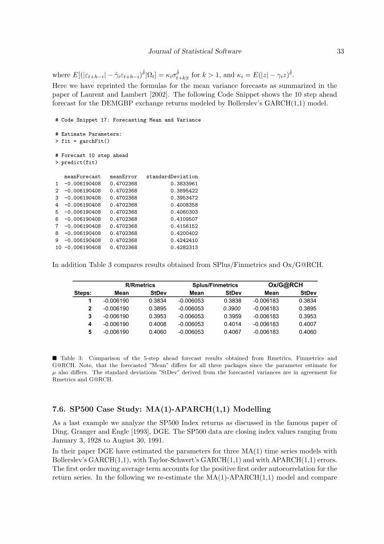
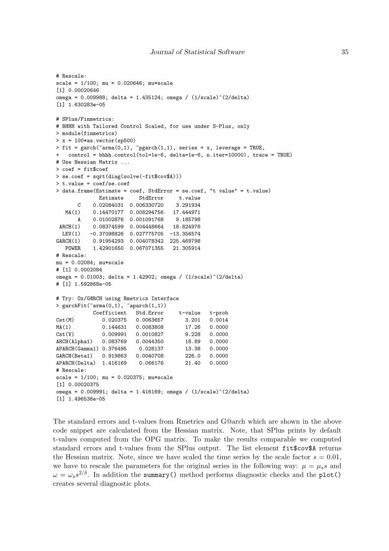


![Package ‘fGarch’ - The Comprehensive R Archive … ‘fGarch ’ November 16, 2017 ... ARCH models, named APARCH, introduced by Ding, Granger and Engle [1993]. The APARCH models](https://img.dokumen.tips/doc/110x75/5ab66e3b7f8b9a0f058dc108/package-fgarch-the-comprehensive-r-archive-fgarch-november-16.jpg)
![MODEL ARCH/GARCH UNTUK MENGETAHUI PERUBAHAN …repository.its.ac.id/2070/7/1213100003-Undergraduate-Theses.pdf · ARMA([43],[43]) serta dari GARCH(2,2) menjadi GARCH(1,1). Kata Kunci](https://img.dokumen.tips/doc/110x75/5cfb798e88c993a9098b6f62/model-archgarch-untuk-mengetahui-perubahan-arma4343-serta-dari-garch22.jpg)
![Analysis of Systemic Risk: A Vine Copula- based ARMA-GARCH … · ARCH model to the generalized ARCH (GARCH) model. Chen and Khashanah [5] implemented ARMA (p, q)-GARCH (1, 1) with](https://img.dokumen.tips/doc/110x75/5accda217f8b9aad468d2abd/analysis-of-systemic-risk-a-vine-copula-based-arma-garch-model-to-the-generalized.jpg)