ARIPAR 5.0: Getting Started Manual Software Tool for Area Risk Assessment and Management

EUR 24963 EN - 2011

The mission of the JRC-IPSC is to provide research results and to support EU policy-makers in their effort towards global security and towards protection of European citi-zens from accidents, deliberate attacks, fraud and illegal actions against EU policies. European Commission Joint Research Centre Institute for the Protection and Security of the Citizen Address: S. Contini, EC JRC Ispra (VA) Italy E-mail: sergio.contini@jrc.ec.europa.eu; Tel.: +39 0332 789 217 Fax: +39 0332 785 145 http://ipsc.jrc.ec.europa.eu/ http://www.jrc.ec.europa.eu/ Legal Notice Neither the European Commission nor any person acting on behalf of the Commis-sion is responsible for the use which might be made of this publication.

Europe Direct is a service to help you find answers to your questions about the European Union

Freephone number (*):

00 800 6 7 8 9 10 11

(*) Certain mobile telephone operators do not allow access to 00 800 numbers or these calls may be billed.

A great d eal of additional information on th e European Union is available on the Internet. It can be accessed through the Europa server http://europa.eu/ JRC 67147 EUR 24963 EN ISBN 978-92-79-21478-3 ISSN 1831-9424 doi:10.2788/80449 Luxembourg: Publications Office of the European Union, 2011 © European Union, 2011 Reproduction is authorised provided the source is acknowledged Printed in Italy

Getting Started

3

The different versions of the ARIPAR software is the result of the initiative taken in 1995 by three organisations: the Institute for the Protection and Secu-rity of the Citizen of the Joint Research Centre of the European Commission (EC-JRC-IPSC), the Civil Protection Service of the Emilia Romagna Region (ERR), and the Chemical, Minerary and Environmental Technologies Engi-neering Department of the University of Bologna (DICMA). The general methodology resulted form the outcome of the ARIPAR project (“Analysis and Control of the Industrial and Harbour Risks in Ravenna’s Area”) carried out in the period 1988-1992. This manual refers to Version 5.0 of the ARIPAR software developed on a new GIS platform: ESRI ArcGIS 9.3, and contains several improvements of the previous versions, which run under ARCView 3.3. Contributors to the development of the ARIPAR 5.0 software (in alphabetical order): Binda M3, Contini S2, Fabbri L2 In addition to the above contributors, other colleagues played a significant role in the development of the ARIPAR methodology, in the development of the previous versions of the software, and in the application to real cases which provided an important feedback for improvement. These are listed hereunder (in alphabetical order): Antonioni G1,Bellezza F2, Cozzani V1, Dondi C4, Egidi D4 , Giannotti E3, Uguccioni G5, Spadoni G1 A Technical Committee, involving the three aforementioned organisations, supervises the activities related to the software development, including the dis-tribution policy. 1. DICMA, 2. EU-JRC-IPSC, 3. THS, 4. ERR, 5. SNAM Progetti

Getting Started

4

Getting Started

5

Getting Started

6

Table of Contents

Background 8

Report Structure 10

1. INTRODUCTION TO ARIPAR 5.0 12 1.1. The ARIPAR methodology 12 1.2. System architecture 16 1.3. The area risk analysis procedure 19

1.3.1. Check of Configtouration parameters. 22 1.3.2. Preparation of the (background) map of the impact area 22 1.3.3. Set the Time periods 22 1.3.4. Set the meteorological aggregations 23 1.3.5. Meteorological data 23 1.3.6. Description of the population distribution 23 1.3.7. Description of the point risk sources (Fixed installations) 24 1.3.8. Description of the linear risk sources (Transport of dangerous substances) 24 1.3.9. Description of the calculation grid 25 1.3.10. Risk calculation for selected sources 25 1.3.11. Area Risk recombination for selected sources 25 1.3.12. Risk representation: Local, Individual and Societal Risk 26 1.3.13. Importance analysis 26 1.3.14. Representation of Damage Zones 26

2. INSTALLATION AND INITIALIZATION PROCEDURES 27 2.1. Hardware and software requirements 28 2.2. Installation 28 2.3. Compatibility with operating systems 29 2.4. Preliminary Operations 29 2.5. Execution 29

3. SAMPLE CASE 1: DATA NAVIGATION 30 3.1. ARIPAR System Query 30

3.2. Display Data 34 3.2.1. Display area risk figures 34

3.2.1.1. Source Risk Calculation 35 3.2.1.2. Local Risk – Point Representation 36 3.2.1.3. Local Risk – Grid Representation 38

Getting Started

7

3.2.1.4. Local Risk – Contours 40 3.2.1.5. F-N Cumulative Curves 41 3.2.1.6. I-N Histogram 43 3.2.1.7. Risk Source Importance 44 3.2.1.8. Risk Source Importance (N) 44 3.2.1.9. Point Local Risk Contributors 45 3.2.1.10. Accident Damage Curves 46

3.3. Remove Risk Themes 47

4. HOW TO PERFORM A RISK ANALYSIS 48 4.1. Open a new project 48 4.2. Preparing the impact area map 50

4.2.1. Map formats 50 4.2.2. Background grid 53

4.3. Check/Set Configuration Data 54 4.3.1. The Tables menu 54 4.3.2. Time periods 55 4.3.3. Meteorological Aggregation 55 4.3.4. Meteorological data 56 4.3.5. Population Categories 58 4.3.6. Land Use 59 4.3.7. Dispersion Data 60 4.3.8. Transport data 62 4.3.9. Outcome Type 63 4.3.10. Initiating Events 63 4.3.11. F-N Parameters 64

4.4. Description of the population distribution 65 4.4.1. Draw zones for the distributed population 65 4.4.2. Vulnerability Centres 68

4.5. Description of Plants, Roads and Railways 69 4.5.1. Plants 69 4.5.2. Drawing Roads 70 4.5.3. Drawing Railways 70

4.6. Description of risk sources 71 4.6.1. Accidents in the plant 71 4.6.2. Accident during road transport of Ammonia 75 4.6.3. Accident during transport of Acrylonitrile by railways 79

4.7. Calculation of the Area Risk 80

Getting Started

8

Background

Over the last decade, quantified risk assessment (QRA) techniques have in-creasingly been used for land use planning and risk-informed decision-making. This has particularly been the case in Europe, where high population densities, together with a high degree of industrialisation, has forced decision-makers to develop methods for evaluating and managing the risks. An example of this is given by the area risk studies conducted in Italy since 1988, when the Italian Department for Civil Protection, together with Regione Emilia Romagna, started the ARIPAR project (Analisi e controllo dei Rischi Industriali e Portuali dell'Area di Ra-venna, i.e. Analysis and Control of the Industrial and Harbour Risk in the Ra-venna Area). The main outcome of the ARIPAR project was the development of a methodology and the related software tool for area risk assessment. Spe-cifically, this tool incorporated the analytical knowledge the existing situation in the Ravenna area with respect to risk sources, vulnerability resorts and emer-gency control centres, and it produced quantitative estimate of the risks in the Ravenna area through the development of an "area risk reassembling module" to quantify the risk connected with storage, process and transportation of dan-gerous substances present on site. As a follow up it was possible to suggest priority interventions to mitigate the consequences of potential accidents in the area and to establish appropriate criteria for the implementation of both pre-vention and emergency actions. The ARIPAR methodology and the first software prototype was developed by the Company Consortium that was charged of the technical development of the project, i.e. Snamprogetti, NIER Ingegneria, and DAM, and subsequently op-timised by the Chemical, Minerary and Environmental Technologies Engineering De-partment (DICMA) of the University of Bologna. This prototype was solely ap-plicable to the area of Ravenna, since all the input data for risk assessment, which are problem-specific, were incorporated within the software. In 1995, an agreement between the Joint Research Centre of the European Commis-sion (JRC), Ispra Establishment, Italy, and the Civil Protection Service of the Regione Emilia Romagna (CPS-REM) led to the development, with the technical collabo-ration of DICMA (acting as consultant of CPS-REM), of the first Windows version of the ARIPAR software (ARIPAR 1.0). The main intention was also to produce a software tool for risk analysis which was applicable to other in-dustrial areas. Within the same agreement, two other versions of the software were developed (ARIPAR 2.0 and ARIPAR 3.0). Some aspects of the compu-tational modules and related databases were also improved by Snamprogetti – Health Safety and Environment service (HSE), on behalf of CPS-REM and with the scientific supervision of DICMA.

Getting Started

9

Version 4.0 of ARIPAR, issued in 2004, was a significant improvement over the previous version 3.1. Improvements concerned e.g. the re-engineering of the risk analysis modules written in C++, the full integration of the GIS inter-face with the analysis modules, and the ranking of risk sources. The new ver-sion was about 30 times faster than 3.1. Since 2004 additional capabilities have been implemented even further. These were recently integrated in ARIPAR 5.0, a completely new version, which has experienced the migration from ArcView to ArcGIS, strictly necessary because of the phase-out of ArcView. In addition, ARIPAR 5.0 incorporates a com-pletely new accident consequence module based on a 2D grid and a specific import function from ALOHA-type data. This new feature is particularly im-portant because it allows overcoming the limitation of the previous linear in-terpolation module for consequence assessment data, which has been main-tained as an optional method, to guarantee the full compatibility of the new version with previous projects. Finally ARIPAR 5.0 is characterised by a redes-igned and optimised input window, a more powerful project browser, and an automatic generation module of accident types in railways transport.

Getting Started

10

Report Structure

This Getting Started manual has been written with the aim of making the user confident with the use of ARIPAR 5.0 by letting him/her to practice the most frequent commands through their application to two sample cases. The ac-companying Reference Manual gives an exhaustive description of all com-mands. The present manual is organised as follows. Section 2 contains a brief descrip-tion of the main features of the ARIPAR methodology and of the risk analysis procedure implemented in the homonym software. Section 3 gives the instruc-tion for the installation of the software. In section 4 all commands for data navigation are described with reference to a sample case; the repeated use of these commands allow beginners to rapidly become familiar with the user in-terface. In section 5 the risk analysis procedure is described with reference to another sample case for which data are delivered together with the software; thus the user, by following this exercise can see the type of data, how to enter them, how to run the modules for calculating the risk due to fixed installations and the transport of dangerous substances.

Getting Started

11

Getting Started

12

1. INTRODUCTION TO ARIPAR 5.0

1.1. The ARIPAR methodology

The ARIPAR methodology is based on a set of procedures aimed at assessing- in quantitative terms - the risks connected with processing, storage and trans-portation of dangerous substances in industrial areas. The risk quantification procedure develops through the evaluation, for all risk sources, of the acci-dents’ occurrence frequency and of the magnitude (number of casualties) caused by such events. Magnitude and likelihood can be combined to produce risk measures. The fol-lowing figures are considered as risk indicators.

Local risk: the expected frequency of the reference damage (death of people) occurring as a consequence of any accident, to a person who is permanently occupying (24 hours a day for one year) a certain point of the area, with no possibility of being sheltered or evacuated. Hence the local risk does not depend on the population distribution, i.e. it is the same. It is a figure useful for characterising the risk in a given location. In ARIPAR the local risk has two types of representation, as risk con-tours, on the overall geographic area, and as a histogram showing, for a given location x, y, the risk value and the contribution of the different risk sources.

Individual risk: the definition is similar to the previous one, except that in the evaluation of the reference damage probability some other vari-ables are considered, i.e. the average exposure time, location, and possi-ble protections like staying indoors. It is a figure that is useful in charac-terising the risk of a site in relation to its use. The common form of presentation of the individual risk is the risk contour plot. Places of particular vulnerability (e.g., schools, hospitals, and supermar-kets), where there is a significant concentration of people are also con-sidered in the individual risk calculation. The Societal Risk addresses the number of people who might be af-fected by hazardous incidents. An F-N curve is a plot of the inverse cumulative frequency (F) of accidents from all the different sources ca-pable of causing the reference damage to a number of people greater than or equal to N. The F-N curve is a figure useful for characterising the societal consequences of possible accidents. The frequency F natu-rally decreases as the number of fatalities increase. The limits of risk ac-

Getting Started

13

ceptability are shown as two parallel straight lines on the same diagram, with an area between them in which risk reduction is desirable. Another useful representation of the societal risk is by means of the I-N histogram, showing the number N of people exposed to an individual risk within the range I, (for example the range 10-6 - 10-5 lethal events/yr.). It is another figure that is useful in characterising the socie-tal exposure to the risk.

The mentioned “impact area” could be defined as the area within which the consequences of potential accidents are to be studied. The extension of the impact area is selected on the basis of considerations about the a-priori judge-ment of the impact of potential accidents on the population as a whole. When considering fixed installations it is quite simple to define the impact area exten-sion, whereas the risk due to the transport of dangerous substances, which goes outside the impact area, may push the analyst to further extend such area. However, there is no doubt that the higher quantity of transported substances, hence the higher risk, is around fixed installations. Within the impact area data to be collected concern first of all the population distributed on the overall area, population concentrated into vulnerability cen-tres (e.g., schools, hospitals, and supermarkets), high vulnerability resorts, as well as the transport networks. In the framework of the application of the ARIPAR system the procedure for area risk analysis develops through the following four main steps, which are schematically represented in Figure 1.1. A. Description of the geographical area of interest The first step of the methodology is the definition of the source area, where the risk sources are located, and the description of the impact area, where the risk has to be determined. The impact area must be described by means of ter-ritorial data e.g. population density, high vulnerability resorts, transport net-works. In addition, the risk analysis is performed by considering the solar year as reference. Since both the meteorological conditions and the population dis-tribution vary with time, it is necessary to subdivide the whole year into periods in which both the meteorological data and the population distribution can be considered constant with an acceptable degree of approximation.

Getting Started

14

Frequency estimation

Accident consequences

OFF LINE ANALYSIS

Vulnerability Centres

Demography

Impact Areamap

Meteorology

IMPACT AREA DATA COLLECTION

AREA RISK ASSESSMENT

ARIPAR SYSTEM

Local and Individual Risk

Societal Risk Risk Source Importance

Plants

SOURCE AREA DATA COLLECTION

Figure 1.1: Schematic diagram of the ARIPAR process

Getting Started

15

B. Identification and Inventory of accident risk sources Storage, process plants and transport of dangerous substances define the risk sources, which exist on a territory where residents, workers and tourist live and can be subject to the consequences of accidents. Data collection has to be car-ried out with particular care and, therefore, it represents one of the most ex-pensive phases. Data related to dangerous substances -which are stored, proc-essed and transported- are collected in order to get a detailed knowledge of their presence and flow in the impact area. C. Off-line analysis of potential accident scenarios This includes the identification and the evaluation of potential accident scenar-ios (i.e. gas dispersion, fire and explosion events), which are selected for de-tailed analysis. This results in the identification of the ‘top events’ for each risk source present in the impact area. If follows the estimate of their likelihood of occurrence and consequences. This analysis is also a very time-consuming phase of the project, as complex industrial and transport processes must be thoroughly analysed. D. Area risk assessment The aforementioned measures of local, individual and societal risk are used as indicators of the area risk resulting from the aggregation point risk sources (i.e. installations of chemical plants) and linear risk sources (i.e. different transport-types). The ARIPAR methodology uses a powerful numerical procedure able to overcome computational difficulties arising from: • non-symmetric distribution of local and individual risk around

sources, when scenarios depending on wind rose must be simulated; • need to manage a large number of accident scenarios at a time; • presence of linear risk sources, associated with transport of danger-

ous substances (i.e. trucks, trains, ships) or with mass flows (i.e. pipelines), which must be represented by many point sources, which are represented as segments of fixed length.

ARIPAR provides values of local and individual risk, which are calculated in the centre of each cell of a non-homogeneous grid superimposed to the impact area. This grid is constructed for societal risk evaluation purposes, in such a way that the cells resulting from it are densely clustered on the areas where the population density is higher. The accurate choice of cells’ dimension and dis-tribution must be done to assure a good compromise between accuracy of the results and acceptability of computation time.

Getting Started

16

1.2. System architecture

The architecture of ARIPAR 5.0 is schematically represented in Figure 1.2. The system includes the Accident Scenario database containing data on plants, transports and accident scenario. Topographic and thematic maps are managed by the GIS and are not explicitly represented here

The risk analysis input data to be fed into ARIPAR are the frequencies of the accident scenarios and the consequence damage profiles associated therewith, which have to be obtained from external databases and models, respectively. This peculiarity of ARIPAR gives a great flexibility to the risk analysts because it allows the use of any data or models for frequency and consequence assess-ment. For consequence assessment, the damage profiles obtained via external nu-merical codes are normally available in terms of discrete values (i.e. overpres-sure, temperature or toxic concentration) as a function of the distance from the risk source. These sets of data are used by ARIPAR in two different ways: 1) to

Figure 1.2. Schematic diagram of the architecture of ARIPAR 4.5

Risk calculation for each accident

(top event)

Documentsrepository Interpolation of

Damage Curves

Risk aggregation for selected accidents

Individual & Local Risk Contour/Grid

GIS INTERFACE

ACCIDENTSCENARIODatabase

ARIPAR Risk Analysis INPUT DATA Frequency of Accidental Scenarios

Damage Curve (data points) Document

Management module

Getting Started

17

create interpolating functions through a least-square process, which provide the functions representing the spatial distribution of overpressures, thermal radiation and toxic concentrations, 2) to interpolate the data on a user defined 2D grid. The risk on the impact area is calculated for each accident scenario. After-wards, the analyst has the possibility to select a subset of scenarios for which the area risk figures are displayed (i.e. local and individual risk contours, F-N curves, I-N histograms, and risk-source-importance). Thus, it is possible to quickly obtain as many risk maps as the number of sub-selections, e.g. for a given typology of sources, for a single road, a single plant, a single substance, a category of plants, and so on. This approach allows the analyst to focus on some specific risk sources and scenarios to which he/she can be interested in, and to get an overview of the differences amongst the different scenarios in term of their contribution to the overall risk. In addition, for each subset of accident scenarios it is also possible to calculate their associated damage curves, which are displayed by selecting user-defined thresholds. Results are graphically represented on the topographic map of the impact area. A new module has been developed to rank risk contributors. This module pro-vides a figure of the importance of risk for different sources according to their aggregation, e.g. plants, substances, scenarios, and top events. This provides a ranking of the selected elements in terms of their importance. Figure 1.3 shows the main steps of the area risk analysis implemented in ARIPAR, which explain the different parameters that are requested in a risk study. In particular, the aim is to calculate the overall risk on the selected im-pact area. This is performed by the ‘Risk Calculation’ modules, which requires a number of input information such as the frequency of all significant accident scenarios (both for fixed installations and for transport of dangerous sub-stances), the population distribution in the area, and the results of the conse-quence assessment in terms of the potential of the selected scenarios to pro-duce harm to the human life. This last aspect (‘Vulnerability analysis’) requires the knowledge of the effect of the involved substances on human beings and other information such as the possible protection measures in place, and the time of exposure.

Getting Started

18

Consequence analysis results for all aggregated meteo data

Vulnerability analysis

Meteo data aggregations

Consequences in each point of the grid

Meteo data

Population distribution Accident scenario

Frequency

Parameters for road transport

Number of vehicles

Length of road stretch

Risk Calculation

Probability Cut off

Day/night and season probability

Frequency of initiating event

Conditional frequency outcome

Exposure times

Probit or criteria

Mitigation coefficients

Cut off thresholds

Road Transport Frequency

Substance

Figure 1.3. Flow diagram of the main data set used in ARIPAR

Getting Started

19

1.3. The area risk analysis procedure

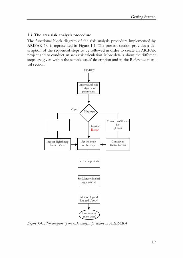
The functional block diagram of the risk analysis procedure implemented by ARIPAR 5.0 is represented in Figure 1.4. The present section provides a de-scription of the sequential steps to be followed in order to create an ARIPAR project and to conduct an area risk calculation. More details about the different steps are given within the sample cases’ description and in the Reference man-ual section.

Figure 1.4. Flow diagram of the risk analysis procedure in ARIPAR 4

Import digital map In Site View

Digital Raster

START

Set the scale of the map

Meteorological data (edit/copy)

Set Meteorological aggregations

Paper

Convert to Shape-file

(if any)

Import and edit configuration parameters

Convert to Raster format

Set Time periods

Map type

Continue A (next page)

Getting Started

20 Continue

B

Generate the layer of calculation grid

Risk calculation for selected sources

Fitting consequence data

A

Draw Vulnerability Centres (VC)

Enter population presence data

Draw polygon. Enter density/population

Enter scenario data

Draw sources and enter attributes

Enter scenario data

Draw risk sources for transport.

Enter attributes

Enter VC attributes

Describe population distribution

Describe Risk sources for Plants Point risk source con-

sequence analysis out-put file

For all polygons covering inhabited areas

For all Vulnerability centres

Draw polygons of fixed installations.

Enter attributes

Fitting consequence data

Transport risk source consequence analysis

output file

Describe Risk sources for Transport

Describe Vulnerability centres

Risk calculation

Vulnerability data

Selection of risk sources (set S)

Draw road, rail, pipe, and channel nets.

Enter attributes

Getting Started

21

Grid for polygons of population distribution Background grid Location of Vulnerability centres

END

Area risk recombination

B

Select the set K of risk sources (K ⊆ S)

Societal Risk

F-N Curves Source-type Im-

portance I-N histograms

Risk source Importance analysis

Source ranking

Local Risk

Risk profiles Risk contours

Risk Grid Point Risk

contributors

Risk points

Individual Risk

Risk profiles Risk contours

Risk Grid Point Risk

contributors

Risk points

Reporting of area risk analysis

Getting Started

22

1.3.1. Check of Configuration parameters.

In ARIPAR 5.0 a set of default parameters are automatically uploaded at the creation of a new project. Before starting with the analysis it is, therefore, nec-essary to check whether the default parameters are valid also for the area under study. As shown in figure 1.4 these parameters concern, e.g.: − Population categories; − Population presence; − Accidents exposure time; − Mitigation parameters; − Road types; − Classification of Land use zones and population density; − Classification of vulnerability centres; − Classification of initiating events;

1.3.2. Preparation of the (background) map of the impact area

The map of the impact area has to be uploaded into ARIPAR. This can be done using two alternative formats:

Raster format. If the map is available in digital form and it is already geo-referenced, it can be directly imported into ARIPAR without any further elaboration. More frequently, however, the area map is available on paper. In this case, it has to be scanned and then scaled using the ARIPAR Map Scaling Utility de-scribed in the Reference Manual. Vector format. The impact area map may be available in one of the many CAD vector formats compatible with ArcGIS. In this case the CAD map is converted into the ESRI shapefile format for further editing. Finally the vector map is converted into the raster format. These operations are described in the Reference Manual.

1.3.3. Set the Time periods

The reference time used by ARIPAR for the area risk analysis is 1 year. During this period of time the meteorological conditions are obviously not constant, they change indeed in the different seasons and during day and night. In this phase the analyst can subdivide the reference period into sub-periods, accord-ing to the meteorological data values and the movement of people, which in-fluence the population density. These sub-periods should not necessarily have

Getting Started

23

the same duration and they will be defined by the analyst according to the data in his/her possession and the desired level of accuracy for the analysis. For instance, the reference period could be subdivided into the four seasons ac-cording to the meteorological data; the summer period could be further split into two sub-periods to account for a different population presence (e.g., tour-ists), and so on.

1.3.4. Set the meteorological aggregations

Some consequence models (i.e. gas dispersion) require the knowledge of mete-orological information such as the wind speed and Pasquill stability class. The damage profiles resulting from them are usually given as a function of the downwind direction and are strictly dependent on the above parameters. For ARIPAR the consequence analysis is performed off-line using external tools and at the beginning of the study it is necessary to establish which of the ag-gregations of wind speed - Pasquill stability class have to be considered. In par-ticular, the examination of the meteorological conditions leads to the definition of the most representative reference aggregations and time periods. Clearly, the highest is the number of aggregations the most accurate is the risk estimate. However, by increasing the number of aggregations the amount of information and of calculations required can become very demanding, which makes the costs of the overall analysis much higher.

1.3.5. Meteorological data

For each Pasquill stability class, the impact area’s wind rose is provided. This gives the probability of wind directions for 16 sectors of 22.5 degrees. For each reference sub-period, it will therefore be necessary to define a number of wind roses for each aggregation. ARIPAR allows representing the wind rose(s) in graphical form. Default setting for the wind rose is a uniform distribution.

1.3.6. Description of the population distribution

The population can be seen as uniformly distributed into small areas delimited by polygons, which identify residential, industrial, and commercial zones. Some attributes are then directly associated with each polygon (i.e. name, type, popu-lation density). Besides, the polygon is associated with a grid characterised by cells with user-defined size, which is used by ARIPAR to calculate and display the risk. Population can also be represented as concentrated into the so-called Vulnerability Centres (VC), represented as point in the map, where a significant amount of people is supposed to be present for certain periods of time. Typical Vulnerability Centres are e.g. hospitals, churches, commercial centres, airports, and schools. Also population type can be categorised by the user (e.g. resident,

Getting Started

24

workers, tourists, etc.) according to their presence on site i.e. either temporary or permanent. The percentage of each category is then assigned for each poly-gon zone/VC. This set of data will allow mapping the risk for a specific cate-gory or for multiple categories.

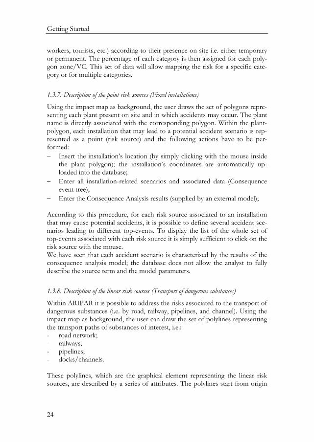
1.3.7. Description of the point risk sources (Fixed installations)

Using the impact map as background, the user draws the set of polygons repre-senting each plant present on site and in which accidents may occur. The plant name is directly associated with the corresponding polygon. Within the plant-polygon, each installation that may lead to a potential accident scenario is rep-resented as a point (risk source) and the following actions have to be per-formed: − Insert the installation’s location (by simply clicking with the mouse inside

the plant polygon); the installation’s coordinates are automatically up-loaded into the database;

− Enter all installation-related scenarios and associated data (Consequence event tree);

− Enter the Consequence Analysis results (supplied by an external model); According to this procedure, for each risk source associated to an installation that may cause potential accidents, it is possible to define several accident sce-narios leading to different top-events. To display the list of the whole set of top-events associated with each risk source it is simply sufficient to click on the risk source with the mouse. We have seen that each accident scenario is characterised by the results of the consequence analysis model; the database does not allow the analyst to fully describe the source term and the model parameters.

1.3.8. Description of the linear risk sources (Transport of dangerous substances)

Within ARIPAR it is possible to address the risks associated to the transport of dangerous substances (i.e. by road, railway, pipelines, and channel). Using the impact map as background, the user can draw the set of polylines representing the transport paths of substances of interest, i.e.: - road network; - railways; - pipelines; - docks/channels. These polylines, which are the graphical element representing the linear risk sources, are described by a series of attributes. The polylines start from origin

Getting Started

25

to destination of transport, and are characterised by intermediate vertices cor-responding to change-direction points. During the polylines drawing process, which is simply performed using the mouse on the map, the coordinates of each vertex are automatically uploaded into the database. Obviously, if more paths follow the same physical route, both vertices and corresponding seg-ments are drawn only once. Then, for each scenario, the following actions have to be performed: − Enter all transport-related scenarios and associated data (Consequence

event tree) − Enter the Consequence Analysis results According to this procedure, each polyline representing a transport route can be associated with one or more accident scenarios.

1.3.9. Description of the calculation grid

ARIPAR provides values of local and individual risk, which are calculated in the centre of each cell of a non-homogeneous grid superimposed to the impact area. This grid is constructed for societal risk evaluation purposes, in such a way that the cells resulting from it are densely clustered on the areas where the population density is higher. The accurate choice of cells’ dimension and dis-tribution must be done to assure a good compromise between accuracy of the results and acceptability of computation time.

1.3.10. Risk calculation for selected sources

The risk for each source is determined at all cells of the calculation grid. The user can decide whether to select the whole set { S } of risk sources for the area risk quantification or to restrict the calculation to the contribution of a subset { K } of the risk sources by excluding the others from the analysis.

1.3.11. Area Risk recombination for selected sources

The determination of the area risk is performed for the selected sub-set{ K } ⊆ { S } of risk sources. In particular the risk contributions from the different scenarios of the selected subset of risk sources are summed up in each cell of the calculation grid. The final result is the overall risk in each grid cell resulting from the K risk sources.

Getting Started

26

1.3.12. Risk representation: Local, Individual and Societal Risk

ARIPAR provides the results of the risk quantification using different risk in-dicators, which can be represented and displayed in different ways: Local risk - Risk contours from 1 to 10-10 - Coloured Risk areas (grid representation); - Point risk contributors Individual risk - Risk contours from 1 to 10-10 - Coloured Risk areas (grid representation); - Point risk contributors Societal risk - F-N curves - I-N histograms The risk aversion concept is also included in the analysis.

1.3.13. Importance analysis

A new module has been developed for importance analysis. Besides the histo-grams showing the: - Risk source importance vs. number of causalities (N) - Risk source ranking for a given value of number of causalities (N) Additional capabilities are available allowing the user to rapidly identify the major contributors to the overall risk, which in turn can be used to define pos-sible strategies to reduce the risk in the impact area. In particular, it is now pos-sible to rank the contribution to the area risk for: − different risk source types; − different substances; − scenarios for one or more selected risk source types; − outcomes for one or more selected scenarios; All these results are displayed as F-N curves.

1.3.14. Representation of Damage Zones

For each potential accident it is possible to show the affected area in terms of the associated physical effect. In particular, when clicking on a risk source, it is possible to select the specific scenario of interest and a wind direction. Then ARIPAR visualises the associated damage curves, which are represented as iso-effect curves, calculated for user-defined values (thresholds).

Getting Started

27

Getting Started

28

2. INSTALLATION AND INITIALIZATION PROCEDURES

2.1. Hardware and software requirements

The minimum hardware characteristics are: − Pentium III 500 MHz − 512 Mbytes of RAM memory − 20 Gbytes of disk space ARIPAR runs on Personal Computers under different Windows operating sys-tems. ARIPAR requires the licence of ESRI ArcGIS 9.3 or superior.

2.2. Installation

ARIPAR 5.0 is supplied on CD-ROM. When inserting the CD-ROM, the setup programme starts automatically. The following dialog appears:

NOTE: if the setup does not start automatically double click on the Setup Aripar.exe program located on the CD-ROM. The setup programme checks whether ARIPAR 5.0 or ARIPAR 4.x are already installed. If this is the case, an Update button replaces the Setup button and only the files that need to be up-dated are replaced. If ARIPAR 4.x is present, the system update is automatically performed (i.e. programmes and files). The setup programme creates the ARIPAR working directory and few sub-directories. The dBase driver must be installed per permettere il collegamento con le tabelle ArcGIS. Normally this driver is installed in Windows by default.

Getting Started

29

2.3. Compatibility with operating systems

Many users have tested ARIPAR 5.0 and no compatibility problems have been found with the following operating systems: - WINDOWS 2000 Professional; - WINDOWS XP Professional; - WINDOWS 7 (32-bit) For the 64-bit version of Window 7, some libraries could result as not regis-tered. In such a case it will appear a message referring to this. It is therefore necessary perform a manual registration of the involved libraries by entering as Administrator, or refer to the system administrator to proceed further.

2.4. Preliminary Operations

Verify that in ArcGIS the security level of VBA code be activated as LOW. To do so, i.e. to access the Security dialog, it is necessary to execute the follow-ing actions: - launch ArcMAP; - select “Tools” in the menu, and then “Customize”; - select “Change VBA Security”; - select the option “LOW”; - exit from the dialog by pressing “OK”. ARIPAR 5.0 is compatible with the previous versions ARIPAR 4.x. However when opening a project created using ARIPAR 4.x it is necessary to cancel the theme “Population Area – Point” because it is not used anymore in the new version.

2.5. Execution

There are two alternative ways of running ARIPAR: 1. Open the ARIPAR folder from Desktop and double click on the icon

; 2. Open the Start + Programme + ARIPAR folder and select the ARI-

PAR item;

Getting Started

30

3. SAMPLE CASE 1: DATA NAVIGATION

In order to allow the user to familiarise with the most common ARIPAR fea-tures, a sample case is delivered with the software.

3.1. ARIPAR System Query

The first sample case considers a geographical area of about 80 km2 in which some hypothetical chemical plants are located. Dangerous chemical substances are also transported by road and railways. To start the ARIPAR application double click on the icon located on the ARIPAR desktop folder:

Figure 3.1 The ARIPAR folder The project manager opens the following windows:

Figure 3.2 The Main ARIPAR dialog

Getting Started

31

After the software installation, Sample Case 1 is by default the project that is automatically uploaded into ARIPAR when launched. This is clearly shown in the dialogue box. To run the application click the button: ArcGIS opens with Sample case 1:

The User Interface contains the following main elements:

• the Menu bar; • the Toolbar and the Button bar to rapidly activate frequently-used

commands; • The Table of Content (TOC), which contains all thematic maps (also

referred to as layers or themes). A theme is said to be Selected when it is highlighted in the TOC; click on its name to select it. A theme is said to be Active when the corresponding box is checked; the effect is that it is made visible in the main View.

The Table of Content is shown below:

ARC-GIS

ARIPAR

TOC

The View

Getting Started

32

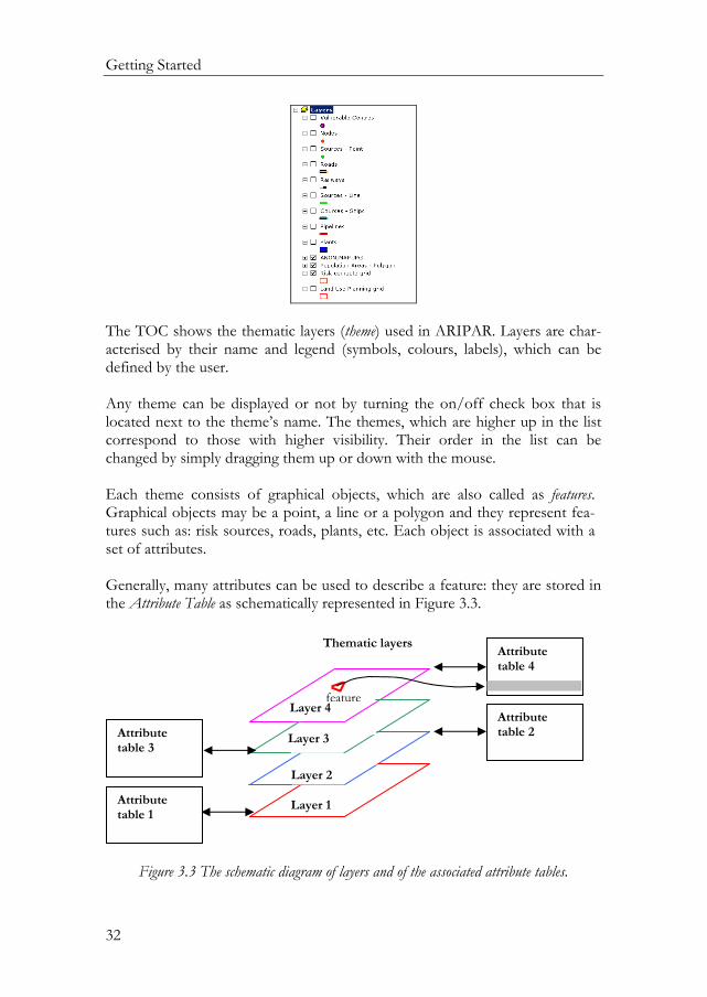
The TOC shows the thematic layers (theme) used in ARIPAR. Layers are char-acterised by their name and legend (symbols, colours, labels), which can be defined by the user. Any theme can be displayed or not by turning the on/off check box that is located next to the theme’s name. The themes, which are higher up in the list correspond to those with higher visibility. Their order in the list can be changed by simply dragging them up or down with the mouse. Each theme consists of graphical objects, which are also called as features. Graphical objects may be a point, a line or a polygon and they represent fea-tures such as: risk sources, roads, plants, etc. Each object is associated with a set of attributes. Generally, many attributes can be used to describe a feature: they are stored in the Attribute Table as schematically represented in Figure 3.3.

Figure 3.3 The schematic diagram of layers and of the associated attribute tables.

Attribute table 4

Layer 1

Thematic layers

Layer 4

Layer 3

Layer 2

Attribute table 3

Attribute table 2

Attribute table 1

feature

Getting Started

33

Different thematic maps can be combined if they are correctly aligned, i.e. if they are referenced in the same co-ordinate system. Within ARIPAR themes describe the Topographical map of the impact area, the Population distribu-tion, Plants, Pipelines, Roads, Docks, Railways, Risk Sources, Risk calculation Grid and Vulnerability Points. Attribute tables can be linked together to create hierarchical relationships among themes. In ARIPAR the hierarchical relationships among themes is very simple, as can be seen from figure 3.5. Themes at first level (Land use zones, Vulnerability centres, etc,) are independent, i.e. there is no precedence rule in their construction. Themes at second level, linked to those at first level, indicate that they must be constructed only after the corresponding themes at first level have been completely defined. The hierarchical relationship means also that if e.g. a plant is deleted then the layer with point risk sources is re-moved too, together with the associated Attribute tables and data.

Figure 3.4 Hierarchical relationships among layers in ARIPAR

Themes should be seen as piled one above the other. Those that are placed on the upper part of the TOC have a higher priority, i.e. they are displayed on those with lower priority. For this reason point themes are placed on the top of line themes and these in turn on the top of polygon themes. If raster map are loaded in the top these, if not transparent, must be placed below the theme stack. Drag and drop the desired theme to change its priority. To notice the effect of priority, move the Map layer on the top: all other layers will not be displayed even if they are active, simply because the map being not transparent covers all other themes. A layer must be selected before making any operation on it. Click on the layer to make it active.

Land use zones Plants

Point risk sources

Transport network

Linear risk sources

Vulnerability Centres

Grid for area risk calculation

Getting Started

34

3.2. Display Data

To display data associated to any object of any theme: − Select the layer − Press the tool button − Click on the object of interest

With this simple sequence of commands the user can display the data associ-ated to any feature in any theme. For instance, the application of the above commands to e.g. the sources-Point layer, and then on a particular source e.g. a plant, shows the data in the follow-ing dialog.

Try several times the use of this simple three-step procedure to display the dia-log associated to other layers. 3.2.1. Display area risk figures

The results of the risk analysis of each source are stored into the database for further uses. These results are then properly combined with the results from other sources to determine the area risk figures. The Risk menu controls the area risk assembling module and the display of the results obtained. It contains the following items.

Getting Started

35

3.2.1.1. Source Risk Calculation The first operation for area risk calculation is the selection of the risk sources. The Source Risk Calculation item of the Risk menu opens the following dialog:

The left pane contains all risk sources described on the impact map. The Virtual source step (m) is the length in meters used for the determination of the risk due to the transport of dangerous substances. A smaller value increases the running time but increases the precision in assessing the risk; In general 50 m seems a good compromise of accuracy of results and running times. This has been selected as a default value. Note that the minimum acceptable value is set to 20m.

Getting Started

36

The Global Grid step (m) appears only if the calculus mode on uniform grid was previously selected within the Project management ->Set ArcGIS parameters sub-menu in the main ARIPAR dialog. Also in this case a default value of 50 m is considered. To select all risk sources (as shown in the above dialog) click the button: To execute the risk analysis for all selected sources it is necessary to click the

button. When pressed the calculation module is launched and the following dialog is displayed from which the user can see the progress of the analysis:

The program processes all risk sources, whose identifier are included in the Selected Risk Sources pane, showing in real time the progresses in the analysis; the following data are shown: - the identifier of the Source currently processed; - the number of Sources already processed; - the source step in case of linear risk source. At the end of the processing a message is displayed. The computation can be interrupted at any time by clicking the STOP button.

3.2.1.2. Local Risk – Point Representation With the selection of this item the local risk is determined for the whole area by recombining the risk from all the previously selected sources. The local risk is calculated on each predefined point, i.e. grid cell and vulnerability centres. These values are the same as those of the local point risk. In this case the risk at any point is represented on the map of the impact area. A point to note is that this feature can be disabled within the Project management ->Set ArcGIS pa-rameters submenu in the main ARIPAR dialog. When selecting the Local Risk – Point Representation item the Area Risk Ag-gregation dialog is displayed, as shown in the following picture. This is the main dialog for selecting the sources of risk to be recombined to produce the risk maps. It contains five panes containing: − The list of Substances used in the accident scenarios; − The list of plants and transport means described in the impact area map;

Getting Started

37

− All risk sources − All top (accident) defined; − All population categories considered in the study. Apart from the last one whose items that cannot be selected, the others can be used to produce a lot of risk maps. To make a pane selectable, just click in the All check box. For a multiple selection of items use the Ctrl key. For instance, with the selection of one or more substances ARIPAR automati-cally identifies all scenarios in which the selected substances are involved and determines the corresponding area risk. If a plant if selected then the Source pane contains all risk sources of that par-ticular plant; the selection of a source makes the list of the corresponding top to appear in the Top pane. After selecting the items of interest click the button to determine the Lo-cal risk:

Getting Started

38

Figure 3.5 Local Risk – Point representation with a risk compute grid of 200m

Different colours correspond to different risk levels. To see the risk map just make the generated Local Risk – Point layer active in the TOC. The present section is also applicable to the representation of the Individual risk is selected within the Project management ->Set ArcGIS parameters submenu in the main ARIPAR dialog.

3.2.1.3. Local Risk – Grid Representation The risk map can also be represented as transparent coloured surfaces (Grid representation). It is convenient to use the Grid representation with a cell di-mension lower than the minimum cell dimension used for the calculation. Consequently the new risk values are obtained from interpolating the values associated with the neighbourhood cells. The interpolation method imple-mented is the Inverse Distance Weighting Power which is expressed by the following equation:

)d/1(

d/)y,x(R=)y,x(R

ki

n

1=i

kii

n

1=i0

∑

∑

where:

Getting Started

39

− i ranges from 1 to the number n of neighbouring points (by default : n=3); − k is the weighting power of di (distance) between Ro(x,y) and Ri(x,y). De-

fault value: k = 2. The greater is k the lesser the influence of the point risk value Ri(x,y) on Ro(x,y)

The power factor k and the number of points n are set in the Agis.ini file. At the selection of the Local Risk – Grid Representation item the Risk Aggregation dialog is not displayed. In fact the risk grid is determined on the basis of the selection made for the calculation of the Risk Points Representation and there-fore a new selection is obviously not possible. For this reason the selection is blocked and the following dialog is displayed to enter the input data for the grid layer calculation.

The following data have to be entered to get the grid representation. − Size of the cell of the grid to be calculated. The size of the interpolated cell

defines the precision with which the risk will be displayed. The cell dimen-sion should not be larger that the smallest calculation sub-grid.

− Minimum risk value to display: i.e. values less than the minimum are not shown; the default value is set to 10-10; this risk threshold is useful e.g. to display on the area map only the zones in which the risk is not acceptable.

Press the OK button: the area risk map, as that represented in Fig 3.6, is gener-ated. To allow the analyst to see the background map the different (coloured) risk zones are semi transparent. In this case the map is 50% transparent. Transparency can be, however, varied bud using the ArcGIS tool Effects by

clicking the button i.e. Show Effects toolbar. In certain occasions, ArcGIS visualise the grid only partially. In that case it is necessary to press F5 from the keyboard to refresh the display. Another possible way of representing the risk map without using the transpar-ency feature for the risk map itself is to make the impact area transparent in-stead, and to drag it above the risk grid in the TOC.

Getting Started

40

Figure 3.6 Local Risk – Grid representation

To know the risk in any cell of the grid: − Select the Risk grid theme; − Zoom-in sufficiently on the sub area of interest; − Press the tool button, or in alternative press and click the mouse

with the left hand key on the desired point on the map; − Click on the grid cell of interest. The present section is also applicable to the representation of the Individual risk is selected within the Project management ->Set ArcGIS parameters submenu in the main ARIPAR dialog.

3.2.1.4. Local Risk – Contours The method used to calculate the risk contours is proprietary, i.e. this algo-rithm was developed to avoid using some specific external features of ArcGIS. In order to obtain good results it is recommended to set the size of the inter-polated cells lower than or equal to the minimum size of the calculation grid. In fact a lower value means higher accuracy in drawing the risk contours, even if the computer time is higher. The following screen shot is the result of the determination of the risk contours for the first Sample Case.

Getting Started

41

Figure 3.7 Local Risk – Contour Representation The present section is also applicable to the representation of the Individual risk is selected within the Project management ->Set ArcGIS parameters submenu in the main ARIPAR dialog.

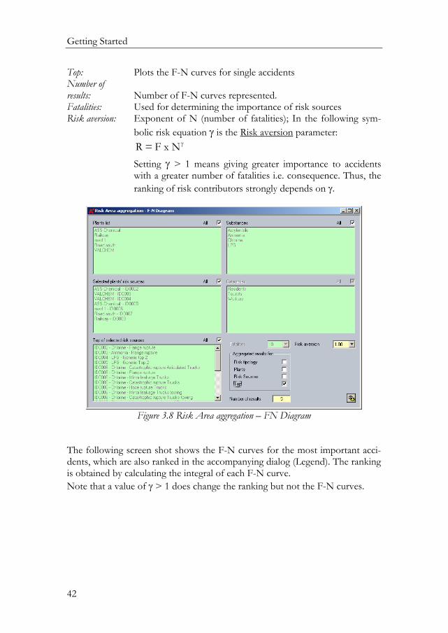
3.2.1.5. F-N Cumulative Curves At the selection of this item from the Risk menu the Area Risk Aggregation dia-log is displayed as shown in fig 3.8. If a selection was previously done it is shown in the dialog: to determine the F-N curves for that selection simply click the Run button . The Area Risk Aggregation dialog contains also the following fields: Risk typology : Plots the total F-N curves for Plants and different Transports; Plants: Plots the F-N curves for a selected type, i.e. fixed installations

or one of the different transport means; Sources: Plots the F-N curves for risk sources;

Getting Started

42

Top: Plots the F-N curves for single accidents Number of results: Number of F-N curves represented. Fatalities: Used for determining the importance of risk sources Risk aversion: Exponent of N (number of fatalities); In the following sym-

bolic risk equation γ is the Risk aversion parameter: γNxF=R

Setting γ > 1 means giving greater importance to accidents with a greater number of fatalities i.e. consequence. Thus, the ranking of risk contributors strongly depends on γ.

Figure 3.8 Risk Area aggregation – FN Diagram

The following screen shot shows the F-N curves for the most important acci-dents, which are also ranked in the accompanying dialog (Legend). The ranking is obtained by calculating the integral of each F-N curve. Note that a value of γ > 1 does change the ranking but not the F-N curves.

Getting Started

43

3.2.1.6. I-N Histogram I-N histograms show the number of people N subject to the Individual risk level falling within a certain risk range (I). The histogram represented below has been determined considering, for the sample case at hand, all risk sources. From this histogram it can easily be seen that e.g. about 1,500 people are sub-ject to risk levels within classes G and H, which correspond to risk greater than 10-5 and most of them live close to the roads transporting dangerous materials.

Getting Started

44

3.2.1.7. Risk Source Importance This histogram shows the importance of the various types of risk sources (plants, railways, harbours, pipes, and roads) vs. the number of casualties N. The value N is defined in the Area Risk Aggregation window.

The value on the ordinates is the yearly accident frequency. This histogram is derived from the F-N curves, i.e. they are the ordinates of the different F-N curves for a given number N of casualties.

3.2.1.8. Risk Source Importance (N) The risk source importance is determined for a given number of casualties N (default value = 10). The following histogram shows that for N=10 the most important contribution in the present case study is given by rail transport.

Getting Started

45

The contribution of risk sources varies with N as can be seen by comparing the above histogram with those that can be obtained setting e.g. N = 100 or 1000.

3.2.1.9. Point Local Risk Contributors This item displays a histogram containing the ranking of risk sources in terms of their contribution to the overall risk (decreasing order of importance) for each point of the area of interest. To get this result select the Point Local Risk Contributions from the Risk menu or click the button. Then click on the point of interest with the left mouse button. The Area Risk Aggregation dialog is displayed. Then clicking the button the following screen shot is an ex-ample of the displayed histogram.

Co-ordinates of the selected point

Population assigned to the point

Risk Source contributions

Getting Started

46

The abscissa reports the Risk source name whilst the ordinate the risk contri-bution of the related source. This feature could be useful for decision-making purposes concerning the reduction of the risk value on the selected point.

3.2.1.10. Accident Damage Curves To display the damage curves for any accident considered in the risk study, select the Accident Damage Curves from the Risk menu (or the tool button, in alternative). Then, in order to get the damage curves for an accident: − select the Source theme; − click with the mouse on any the source of interest The following dialog is displayed

This dialog contains the list of accident scenarios that have been associated with the selected source (in the example of the figure there is only one accident in the list). For visualisation purposes, it is necessary to define the threshold values of the three curves that will be plotted (if different from the default ones), and the wind direction by either using the wind rose or by editing the Wind Direction field. For example, in the dialog the NE direction has been se-lected. Click the button to get the damage curves plotted on the area map as shown below.

Getting Started

47

The dimensions of each damage area can be measured after pressing the tool button. To measure a distance click on the first point with the left mouse button and drag the mouse to the second point: the length of the segment is written on the status bar.

3.3. Remove Risk Themes

All risk themes in the TOC can be removed by selecting this menu item. In order to remove a single theme the following steps are applied: − select the theme; − open the Edit menu; − select the Delete Theme item; − press Yes in the dialog box that is displayed.

Getting Started

48

4. HOW TO PERFORM A RISK ANALYSIS

This section provides all necessary information to perform a risk analysis. This analysis is based on the sequential steps previously represented in Figure 1.4.

4.1. Open a new project

To start a new project it is necessary to execute the following actions : − Open the ARIPAR folder from Desktop;

− Run ARIPAR by clicking the icon: the Browser is displayed:

− Select the Sample Case (this is the Workspace in which the project will be

stored) and then click the New Project icon; the following message ap-pears asking the user where to store the project data and results.

Getting Started

49

No: the project will be stored into C:\Aripar4\SampleCase\ Yes: the Directory Selection windows appear for the alternative directory. For this exercise the first option is to be selected. The following window opens:

Insert the Project name (Trial Case) and click the corresponding Apply button:

Getting Started

50

In the following window select the Open project icon: the ArcGIS opens with an empty as shown in the following dialog:

4.2. Preparing the impact area map

4.2.1. Map formats

The impact area is the geographical area within which the consequences of the accidents are to be calculated. The impact area contains the Risk source area, i.e. the geographical area embedding all risk sources. The choice of the impact area is the first step in Quantitative Risk Analysis: the preliminary choice has to be verified and, if necessary, corrected after executing the analyses. Apparently this implies an iterative procedure, but in practice the first choice is conserva-tive and often includes residential areas that are not subjected to significant risks. Obviously the impact area due to the transport of hazardous substances is larger, since it involves crossed territories, but the traffic density and hence the associated risk is surely higher near industrial sites. On the cartography of the impact area information to be shown are plants, transport routes of dan-gerous substances and the information on population distribution. In order to easily deal with Spatial data, ARIPAR makes use of a commercial GIS (Geographic Information System). Spatial data can be defined as data that are referenced to the Earth, i.e. data that are characterised by their geographic co-ordinates. The type of co-ordinate systems used in ARIPAR is generally longitude-latitude, but it is possible to use other coordinate systems, including local one.

Getting Started

51

The method of representing spatial data in a GIS is through maps, a 2D collec-tion of graphical features (objects) characterised by their x,y co-ordinates. In a GIS spatial data can be represented in vector, or raster formats.

Point

Polyline

Polygon

Lake (Polygon)

Road (Polyline)

(x,y) Vertex

Well(Point) (Polyline)

House (Polygon)

The world picture contains a road, a house, a well and a lake.

World picture

Vector representation

Pixel In the ra ster format each cell is a pixel. The pixel value may be stored in a bit, a bite or two bytes and represents a value in a gray or color scale. Pixels have no associated attribute tables. The raster format is suitable for representing graduated phenomena and images.

Raster representation

Figure 4.1. Different workable data formats in a GIS

Getting Started

52

The fundamental types of entities in vector format are points, lines and polygons. These three entities are used to portray real life objects. For instance, in a chemical plant points may represent e.g. entrance gates, the location of fire-plugs, whereas lines may represent e.g. roads, rivers, electric power lines. Poly-gons may represent buildings, site fence, plant units, residential zones, etc. Each feature can be described by means of some associated attributes e.g. col-our, shape, (numbers, characters, Boolean). Attributes are stored into a record of an Attribute Table managed by the GIS. Other attributes can be added by the user (e,g, plant name, type, etc.) which are stored into the external (to the GIS environment) database tables; all these attributes can be queried and used for calculations. The Raster type data record spatial data in a matrix data-structure in which the smallest logical unit represents a pixel, i.e. a dot on the screen. Raster data for-mats are typical of scanned maps, digital photos and satellite images. The row-column numbers of the array gives the co-ordinates of a pixel on the screen. Values associated to a pixel depend upon the number of bits used to store data. For example, with only one bit the possible values are 1 and 0 (typi-cal of black-and-white scanned maps), whereas with 8 bits, i.e. one byte, they are 28=256, and so on. The information stored in a pixel depends on what the picture represents, e.g. it may represent the light reflected by the object in a satellite image or the brightness value in a scanned map. A pixel does not have an associated attribute table. Attributes can only be associated to the image as a whole. Raster data require more memory space than vector data and for this reason they are normally stored by using data compression techniques. Figure 4.1 graphically describes the differences among vector and raster formats with reference to a sample picture An important requirement in GIS is to work with geo-referenced maps. A map is geo-referenced when each point can be characterised by the geographic co-ordinates: latitude and longitude. Several times the geo=referenced impact area is available at the cartographic services of a local administration, in which case it can be simply imported. To import a geo=referenced map: − Click the tool button: the Add Theme is displayed; − Set “Data Source Type” as Image Data Source;

The Add Theme dialog (browser) allows the user to find the map of interest. The map Anonimap.jpg is located in the directory c:\aripar4\my pro-jects\sample case 1\db. Once found, click OK to import it. Finally acti-vate the layer to display it.

Getting Started

53

However, when the map is available only on paper it must be scanned; in doing so it is always advisable to position the paper on the scanner in such a way that the North of the map can be oriented towards the top of the screen. Windows tools e.g. Photoshop may be used to properly correct the orientation if neces-sary. ArcGIS offers several methods to geo-referencing an image. Refer to the ArcGIS manual for further information.

4.2.2. Background grid

At this stage it is necessary to define a background grid for risk calculations. Within TOC, select the element Risk compute grid and then press button Background grid generation. The following dialog will appear:

The grid area adapts by default to impact map. It is possible to modify the grid area by clicking on Draw grid and by selecting the desired area. By clicking on OK, the background grid will be generated. This is the area there the risk cal-culation will be conducted:

Getting Started

54

4.3. Check/Set Configuration Data

4.3.1. The Tables menu

The Tables menu contains some of the key data, which refer to the area under study, which are necessary to execute the risk analysis. For a new project, ARI-PAR default data for some of these data are automatically uploaded. Before starting the area risk analysis it is important to check whether the default pa-rameters are valid for the case under study. These data concern several aspects such as: population categories, accidents exposure time, mitigation parameters, road transport, land use zones and population density, etc. These data are stored into the ARIPAR database and can be accessed by open-ing the Tables menu:

Figure 4.2.

Getting Started

55

Each item of this menu opens the corresponding editing dialog. Each item ap-pears according to the sequence to be followed for their check/entering, e.g the Time Periods must be defined before the Meteo Aggregation and so on. 4.3.2. Time periods

The risk is calculated on the basis of one year. But during the year some data change, e.g. meteorological conditions and population distribution change. Thus it is important to subdivide the year into two or more periods in which the meteorological conditions and the population distribution can be consid-ered approximately constant. The study for the definition of the number of periods and their duration, which can be different for the different periods, must be set with care. By selecting the Time Periods item from the Tables menu the following dialog appears.

This case consists of two periods: Summer+Spring and Automn+Winter, each lasting 6 months (50% of the year). To insert a period click ; to delete a row select the row (Delete column) and then click the button. The same mechanism of insertion and deletion is also applicable to all other dialogs.

4.3.3. Meteorological Aggregation

With ARIPAR the accident consequence analysis is performed off-line by con-sidering different aggregations of Wind velocity - Pasquill stability class. These calculations can be performed for a single generic direction, e.g. North.

The number and type of aggregations are determined at the beginning of the study on the basis of the meteorological conditions during the reference year. The examination the meteorological conditions lead to the definition of the most representative reference aggregations for each time period. The higher is

Getting Started

56

the number of aggregations the more realistic is the risk estimation. Clearly this is also associated with an increase of the analysis efforts. By selecting the Meteo Aggregation item of the Tables menu the user can enter the most representative aggregations. For this sample case two aggregations are considered: D-5 and F+G-2. Enter these values in the Meteo Aggregation dialog.

4.3.4. Meteorological data

The area risk is calculated by considering a wind rose, for each period, express-ing the wind direction and probability. To enter the Wind roses select the Meteo item of the Tables menu. The following dialog is displayed:

Getting Started

57

The number of Wind roses is equal to the number of the previously defined time periods. This dialog shows for the first period Summer+Spring and for each Aggregation the probability that the wind blows towards the centre of the wind rose. The wind probability must be entered for 16 directions (equal sec-tors of 22.5 degrees). The values in the fourth column (Total) are calculated automatically. The sum must not be greater than 1. For new projects, default values, which correspond to a uniform wind rose, can be obtained by clicking the button which, afterwards turns into . As an example the meteorological values for the second period example Automn+Winter appears as shown below.

These values can also be represented graphically by clicking the button.

Getting Started

58

4.3.5. Population Categories

The determination of the social risk requires the distribution of the population in the impact area. How to describe this distribution will be described later. At this point of the procedure it is sufficient to categorise the population so that the social risk can be determined for each category. Note that the population categories must be defined before entering the population distribution. A population category is defined as that part of the population characterised by the same exposure probability, i.e. the same number of hours per day and day per week of presence in the given point. Example of population categories are: residents, students (associated to school buildings), commercial centre users, workers, etc. Each category is defined by the probability of presence indoor and outdoor during day and night and for each time period. To insert the population categories select the homonym item from the Tables menu. Entre the Population categories residents, tourists, and workers in the dialog; the result is shown below.

Getting Started

59

For each category and for each period the probability of presence indoor and outdoor must be assigned. To do that it is necessary to select the Category (upper part of the dialog) and to insert the data in the lower part. 4.3.6. Land Use

The next step is the definition of the location of the population in the impact area. To facilitate this task ARIPAR offers the user the possibility to draw polygons surrounding different types of land use and to characterise each of them with the following data; − Category of land-use; − Number of people per hectare (100 X 100 meters); − Side of the square cell dimensions in meters for risk calculation. These data are entered in the Land Use dialog selectable from the Tables menu.

Getting Started

60

The above dialog contains six land use categories, the population density and the cell dimensions. The values in the cell dimension depend from the land use type; generally, to improve the precision of risk figures it is recommended to set a cell dimension value directly proportional to the population density. The importance of the cell dimension will be clearer later. 4.3.7. Dispersion Data

In this dialog, along with the next two concerning explosion and fire, a set of data of interest for ARIPAR accepts two types of vulnerability models: Probit equations and Thresholds. These values are already defined for a certain num-ber of toxic and/or flammable substances. Obviously the user can define his/her own data. The dialogs for editing the vulnerability data for dispersion, explosion and fire can be displayed from the Tables menu. As an example the following is the dialog showing the data about chlorine. For each substance the information is limited to the coefficient of the Probit function, which is neces-sary for the determination of the risk. Since more than one Probit can be as-signed to a substance, the user has the possibility to select the preferred one for the risk calculation. The different Probit functions can also be graphically dis-played as shown in the next figure:

Getting Started

61

For this sample case no data have to be entered, because the data for chlorine are uploaded on the ARIPAR database. Similar dialogs can be displayed for explosive and flammable substances. Refer to the Reference manual for a complete description of all fields of the dialog.

Getting Started

62

4.3.8. Transport data

These data are required for the automatic calculation of the road and rail trans-port failure frequencies and shall therefore be given before inputting the road sources in ARIPAR. Refer to the Reference Manual for the description of all fields.

The Cut-off value is the threshold below which the risk is no more calculated for these sources of risk. The release category data refer the frequency of having the corresponding rup-ture type. These Top are automatically generated, as will be seen in the section describing the Risk sources. The accident frequency data for different types of roads are provided in the lower part of the window. Similar data can be entered for the rail transport. Data in this dialog are useful to facilitate the data entry for the calculation of the risk due to the transport of dangerous substances by road and rail. It will be seen later on that the scenario for transport of dangerous substances and the corresponding accident frequency are generated automatically on the basis

Getting Started

63

of the three different ruptures and the accident frequency for different types of roads. For the current sample case these data need not be modified. 4.3.9. Outcome Type

This dialog contains the list of possible outcomes (accidents) with the associ-ated exposure time and mitigation factor. The exposure time is used in the Probit equation to calculate the dose. These default values can be modified for each individual scenario at any moment.

The Heavy Gas Instantaneous release does not contain any editable exposure time as explained later. The program calculates the vulnerability considering an outdoor exposure. To take into account the possible mitigation due to staying indoor the multiplica-tive Mitigation parameter is introduced for each accident type. Being multiplica-tive the value 1 of this parameter means no protection, whereas the value 0 means total pro-tection, with linear behaviour in between. 4.3.10. Initiating Events

This dialog allows entering the accidents initiating event with the associated annual frequency.

Getting Started

64

4.3.11. F-N Parameters

One of the means to graphically represent the social risk is the F-N curve, showing the annual frequency of having N or more fatalities. On the same graph two lines can be represented for dividing the regions Unacceptable-ALARA and ALARA-acceptable risk. ALARA (As Low As Reasonably Achievable) is the region where effort should be considered to reduce the risk. The coordinates of these two straight lines are defined in the F-N Parameter dialog.

Enter your preferred parameters.

Getting Started

65

4.4. Description of the population distribution

4.4.1. Draw zones for the distributed population

The procedure to describe the distribution of the population on the impact area map is composed of the following steps: − Draw the polygon (zone perimeter); − Enter population data for each zone (population density or number of

people); − Enter population composition (categories) − Cell dimension for the risk calculation grid. In order to increase the precision in calculating the risk map, if there is a zone without population (e.g. agricultural, river, wood) placed between an industrial and a residential area it is recommended to describe it with a polygon with a grid cell dimension comparable to the cell dimensions of the two areas (this can also been avoided when using a suitable uniform background grid). To draw a generic polygon: − Select the ‘Population’ Theme on the TOC; − Press the tool button; − Draw the Area boundary on the map covering a populated area. To draw the polygon click with the left mouse button on the first point, then go to the second point and click again, do the same for the third point and for all others up to the last point. Double click to complete the drawing. The following figure shows the polygon generated using the transparent map as background for the industrial area. Since such map is on the top of the TOC it can be seen very clearly. The resulting polygon has the colour and pattern assigned to the “Undefined” element of the Legend, which means that the polygon does not have any data associated. In the following figure the colour and the polygon are only indicative:

Getting Started

66

It may happen that, zooming in, the polygon drawn does not exactly follows the map lines and thus it needs some adjustments. Refer to the ARIPAR Ref-erence manual or the ArcGIS manual to see how to edit a theme. Attributes describing the drawn polygon can be entered as follows: − Be sure that the Population theme is active in the TOC; − Click the tool button; − Click inside the polygon. The following screen shot shows the editing dialog for entering the data con-cerning the selected zone. By selecting the zone type (Industrial in the present case) the default population density value and the number of people are dis-played. By changing one of these parameters the other is automatically adapted on the basis of the zone area. When closing the dialog the colour and pattern of the polygon are changed according to the legend. Note the crosses inside the polygon, which represent the automatically gener-ated grid that will be used later for risk calculation.

Getting Started

67

The above procedure is applied to draw all other polygons. The grids generated inside the polygons are used for calculating the risk, from which the risk contours are then constructed using a linear interpolating algo-rithm. When the impact area has significant portions with no population e.g. woods, sea, mountains, etc, it is important to calculate the risk also on these zones to let the interpolating algorithms to work well. For this reason, if a uni-form background grid was not set, it is advisable to cover the whole impact area with new polygons (classified as “Other” in the Legend Editor, whose cell dimensions are larger than those suggested for inhabited areas. To generate the new grid proceed as follows: − Select the Population Area-Points layer; − Click ; − Draw the polygon covering the area of interest; − Click and then click inside the drawn polygon; − From the Zones dialog that appears select the “Other” element with no

population associated and set the cell dimension.

Getting Started

68

4.4.2. Vulnerability Centres

In addition to the distributed population, singular points can be defined for the calculation of risk, where high concentration of population or particularly vul-nerable people is present (e.g. Hospitals, Schools, and Commercial Centres etc). To insert the date about a Vulnerable Centres (VC): − Select the Vulnerability Centres Theme − Click ; - Click on the location of the Vulnerability Centre: a point is drawn on the map; − Select the Insert Data button and click at the location of the in-

serted centre to open the Vulnerability Centre dialog. The following screenshot shows a VC and the associated dialog, in which the name of the VC and the number of people generally present must be entered.

Getting Started

69

4.5. Description of Plants, Roads and Railways

In this sample we consider as sources of possible accidents a single plant and the transport of dangerous substances by road and rail. 4.5.1. Plants

The procedure to draw a plant polygon is the same as above described for in-habited areas, i.e.: − Select the Plants Theme on the TOC − Click the button − Draw the Area boundary on the map covering the plant surface. To enter the attributes of the plant: − Click the tool button; − Click inside the polygon. The following screen shot shows the dialog for entering data about the drawn polygon.

Getting Started

70

4.5.2. Drawing Roads

The sub road network to be drawn refers only to the transport of dangerous substances. In this sample case we consider the transport of Ammonia. The procedure to draw the roads of interest is as follows: Step 1: draw nodes; − Select the Nodes Theme − Click the button − Click on the origin and destination of the transport; Step 2: draw roads. − Select the Roads Theme − Click the button − Starting from the origin node, draw the road up to the destination node. To insert the data about the road: − Click the tool button; − Click inside the line. A dialog similar to the one shown above for plants is displayed for roads. 4.5.3. Drawing Railways

The sub rail network to be drawn refers only to the transport of dangerous substances. In this sample case we consider the transport of Acrylonitrile. The procedure to draw the railway is similar to that of roads, i.e.: Step 1: draw nodes (see above); Step 2: draw railways. − Select the Railways Theme − Click the button − Starting from the origin node, draw the railways up to the destination

node. To insert the data about the rail: − Click the tool button; − Click inside the line. The following screen shot shows the dialog for entering data about the drawn rail.

Getting Started

71

4.6. Description of risk sources

The risk sources for the present Sample case are represented by accidents in the fixed plant involving the release of ammonia and LPG, by road accidents during the transport of Ammonia, and by rail accidents during the transport of Acrylonitrile. The collection of information about potential accidents in fixed installations is relatively simple when safety reports are available, whereas more complex is the task of finding the amounts of transported substances by road and above all the routes used. The description of accidents follows a two-steps procedure: − Step1: accident location; − Step2: accident description. 4.6.1. Accidents in the plant

In the plant it is supposed that there are two possible accidents involving the release of ammonia and LPG.

Getting Started

72

Step1: accident location − Select the Sources Points Theme in the TOC. − Activate the Input Theme button, selecting − Click on the location, within a Plant boundary, where the accident involv-

ing Ammonia may occur. A new risk source (green point) is generated; − Do the same as above for the accident involving LPG. Step2: accident description. − Click the Insert Data button and then on the first inserted green point:

the first Sources dialog is displayed. Enter the following data about the accident in the dialog shown below: Initiating event: Flange Rupture

Frequency 8.0 10-5 Substance Ammonia Outcome Release – Jet Dispersion Threshold 300 mg/m3 Occurrence 0.4 Mitigation 0.8 Fit file Spf

Now click the Outcome button to get the second dialog. Enter the data in the corresponding fields.

Getting Started

73

The FIT file is a file that contains the results of the consequence analysis per-formed off line. The Spf file can be selected from the Consequence file list. Finally, click the Effects button to open the FIT module. Accept the fitted curve by clicking the Save coefficient values button. With the Save button the coefficients in the NEW column are copied in the CURRENT column and stored in the database.

Click here to open the listof files with the conse-quence analysis results

Getting Started

74

Close the FIT dialog and repeat the above operations by clicking the Effects button for the second period. If the consequence file selected from the list contains the extension “5” after the name then the applied fitting method is different (the number “5” refers to the fact that this is a new feature of the 5.0 version). In these cases the conse-quence analysis results are stored on a 2D grid. How the 2D grid is generated is described in the Reference Manual. For instance, in the following dialog the file name is sacng.5.

Clicking the Effects button the following dialog appears:

Getting Started

75

See the Reference Manual for the description of the commands of this dialog. The same procedure is applicable for entering data about the second accident.

Initiating event 2: Catastrophic rupture

Frequency 2 10-5 Substance LPG Outcome Fireball Threshold 1.6 Kw/m2 Occurrence 0.3 Mitigation 0.3 Fit file Pg38

4.6.2. Accident during road transport of Ammonia

Step1: accident location − Select the Sources Line Theme in the TOC. − Click the button and then click on the road: a green line representing

the linear source is generated between the two nodes. Step2: accident description. − Click the Insert Data button and then on the green line: the first

Sources dialog for the transport of dangerous substances is displayed.

The scenarios for risk transport are generated automatically on the basis of the initiating events defined in the Road Transport Data table (see menu Tables).

Getting Started

76

Select the Road type as Minor road: the associated annual accident frequency is automatically loaded and the Generation of the road traffic Top events dialog is open in which the type of transport means can be described. Enter the data shown in the following screen shot.

When closing this dialog the data about the default initiating event and fre-quencies is displayed.

Now, click the Outcome button to enter the following data:

Getting Started

77

Initiating event 2: Minor leakage Articulated Tracks

Frequency 1.188 10-5 Substance Ammonia Outcome Continuous release Threshold 300 mg/m3 Occurrence 1 Mitigation 0.5 Fit file sacng

The exposure time (60 min) is the default value stored into the Outcome Defini-tion Table Pressing the Effects button for the first scenario the FIT dialog appears with the results of the fitting operation on the data stored in the sacng file.

Again save the data and exit. Repeat this procedure for the second Effect.

Initiating event 2: Catastrophic rupture Articulated Tracks

Frequency 5.94 10-7 Substance Ammonia Outcome Instantaneous release Threshold 300 mg/m3 Occurrence 1 Mitigation 0.5 Fit file spc

Getting Started

78

The exposure time for the catastrophic failure is calculated on the basis of two coefficients as described in the Reference manual. Set the first to 3.4 and the second to 0. Then repeat the above described procedure.

Initiating event 3: Flange rupture Articulated Tracks

Frequency 7.128 10-5 Substance Ammonia Outcome Continuous release Threshold 300 mg/m3 Occurrence 1 Mitigation 0.5 Fit file sacng

The exposure time (60) is the default value stored into the Outcome Definition Table

The following dialog shows the data for the third case.

At this point it remains to run the FIT programme to calculate the interpola-tion functions. This operation is the same as previously seen for the fixed in-stallation.

Getting Started

79

4.6.3. Accident during transport of Acrylonitrile by railways

Step1: accident location − As for road transport, select the Sources Line Theme in the TOC. − Click the button and then click on the railway: a green line represent-

ing the linear source is generated between the two nodes. Step2: accident description. − Click the Insert Data button and then on the green line: the first

Sources dialog for the transport of dangerous substances is displayed.

The procedure is the same as that previously described for fixed installations. Data to be entered are as follows:

Initiating event: Tank Leakage

Frequency 1.0 10-5 Substance Acrylonitrile Outcome Continuous release Threshold 100 mg/m3 Occurrence 1 Mitigation 0.5 Fit file Acrylonitrile

The data entry phase is now completed: the next phase concerns the calcula-tion of the area risk.

Getting Started

80

4.7. Calculation of the Area Risk

The last phase is the calculation of the area risk. Select the Source Risk Calcula-tion from the Risk menu to open the Risk Source selection dialog for calculation. Select all risk sources and click the button to run the risk analysis module.

At the end of the analysis the results can be displayed following the commands described in the first Sample case. The following pictures show the results of the independent calculation of the Local risk for the plant, the road and the rail and then the total risk for all sources. The risk contour representation is shown on the left and the coloured grid representation on the right. Note that the maps shown below are only indicative of the type of results that can be obtained.

Getting Started

81

Figure 4.3 Local risk for the storages of Ammonia and LPG in the plant

Figure 4.4 Local risk for the road transport of Ammonia

Getting Started

82

Figure 4.4 Local risk for the transport of Acrylonitrile by railway

Figure 4.5 Local risk for all sources: plant and transports

Getting Started

83

The next pictures give a typical example of societal risk output produced by ARIPAR, as calculated in the present case study. The first graphs represent the F-N curves corresponding to the different type of risks (plants, transport, etc), and the aggregated risk (red curve). The table underneath provides a ranking of the different risk typology. The second graph is an example of IN diagramme, which provides the number of individuals falling into a certain risk class.

Figure 4.5 Social risk. ARIPAR FN and IN graphs

Getting Started

84

European Commission EUR 24963 EN Joint Research Centre – Institute for the Protection and Security of the Citizen Title: ARIPAR 5.0: Getting Started Manual Editors: S.Contini, L.Fabbri Luxembourg: Publications Office of the European Union 2011 – 86 pp. – 17 x 24 cm EUR – Scientific and Technical Research series – ISSN 1831-9424 ISBN 978-92-79-21478-3doi:10.2788/80449 Abstract ARIPAR is a quantitative area risk assessment tool used to evaluate the risk resulting from major accidents in in dustrial areas where haza rdous sub-stances are stored, processed and transported. It is based on a geographi-cal information system platform (GIS). This tool has already been applied to perform a quantitative area risk assessment in several industrial areas, and it has been demonstrated to be a very powerful tool also for managing in-dustrial risk. ARIPAR 5.0 is the new release of the software, which embeds several new features and improvements, such as a completely new devel-opment platform based on ArcGIS and a much more powerful module for dealing with consequence assessment data. The present document repre-sents the Getting Started manual, which has the aim of ma king the u ser confident with the use of ARIPAR 5.0 by letting him/her to practice the most frequent commands through their application to two sample cases. The ac-companying Reference Manual gives an exhaustive description of all com-mands.

How to obtain EU publications Our priced publications are available from EU Bookshop (http://bookshop.europa.eu), where you can place an order with the sales agent of your choice. The Publications Office has a worldwide network of sales agents. You can obtain their contact details by sending a fax to (352) 29 29-42758.

The mission of the JRC is to provide customer-driven scientific and technical support for t he conception, development, implementation and monitoring of EU policies. As a service of the European Commission, the JRC functions as a reference centre of science and technology for the Union. Close to the pol-icy-making process, it serves the common interest of the Member States, while being independent of special interests, whether private or national.

LB-N

A-24963-EN

-N