Arie Verhoeven [email protected] · PDF file6 Linearized theory of elasticity Arie Verhoeven May 24 ... Airy stress function For plane strain with no body forces, the equilibrium equations

/centre for analysis, scientific computing and applications

Introduction Plane elasticity Three-dimensional elasticity Summary

Linearized theory of elasticity

Arie [email protected]

CASA Seminar, May 24, 2006



Seminar: Continuum mechanics1 Stress and stress principles Bart Nowak March 82 Strain and deformation Mark van Kraaij March 293 General principles Ali Etaati April 124 Constitutive equations Godwin Kakuba April 195 Fluid mechanics Peter in ’t Panhuis May 36 Linearized theory of elasticity Arie Verhoeven May 247 Complex representation Erwin Vondenhoff June 7

of the stress function8 Principles of virtual work Andriy Hlod June 219 The boundary element method Zoran Ilievsky June 28



Outline

1 Introduction

2 Plane elasticityRectangular coordinatesCylindrical and polar coordinates

3 Three-dimensional elasticityDirect solution of Navier’s equationExamples

4 Summary



Outline

1 Introduction



4 Summary



The Cauchy stress tensor

For a linear elastic solid we have the identity:

TJi(X, t) = TJi(x + u(x, t)).

In terms of Cartesian components, the first Piola-Kirchhoff stresstensor T 0

Ji is related to the Cauchy stress Tri at the points x = X + uby

T 0Ji =

ρ0

ρ

∂XJ

∂xrTri . (1)

The displacement-gradient components are small compared to unity.The equations of motion in the reference state are given by

∂T 0Ji

∂XJ+ ρ0b0i = ρ0

d2xi

dt2 . (2)



Field equations

Field Equations of Linearized Isotropic Isothermal Elasticity

3 Eqs. of Motion ∂Tji∂Xj

+ ρbi = ρ∂2ui∂t2 (3)

6 Hooke’s Law Eqs. Tij = λEkkδij + 2µEij (4)6 Geometric Eqs. Eij = 1

2

(∂ui∂Xj

+∂uj∂Xi

)(5)

15 eqs. for 6 stresses, 6 strains, 3 displacements

The two Lamé elastic constants λ and µ, introduced by Lamé in 1852,are related to the more familiar shear modulus G, Young’s modulusE , and Poisson’s ratio ν as follows:

µ = G =E

2(1 + ν)and λ =

νE(1 + ν)(1− 2ν)

.



Boundary conditions

1 Displacement boundary conditions, with the threecomponents ui prescribed on the boundary.

2 Traction boundary conditions, with the three tractioncomponents ti = Tjinj prescribed at a boundary point.

3 Mixed boundary conditions include cases where

1 Displacement boundary conditions are prescribed on a partof the bounding surface, while traction boundary conditionsare prescribed on the remainder, or

2 at each point of the boundary we choose local rectangularCartesian axes Xi and then prescribe:

1 u1 or t1, but not both,2 u2 or t2, but not both, and3 u3 or t3, but not both.



Navier’s displacement equations

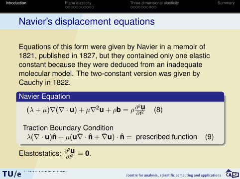
Equations of this form were given by Navier in a memoir of1821, published in 1827, but they contained only one elasticconstant because they were deduced from an inadequatemolecular model. The two-constant version was given byCauchy in 1822.

Navier Equation

(λ+ µ)∇(∇ · u) + µ∇2u + ρb = ρ∂2u∂t2 (8)

Traction Boundary Conditionλ(∇ · u)n + µ(u∇ · n + ∇u) · n = prescribed function (9)

Elastostatics: ∂2u∂t2 = 0.



Outline

1 Introduction



4 Summary



Outline

1 Introduction



4 Summary



Plane elasticity (1)

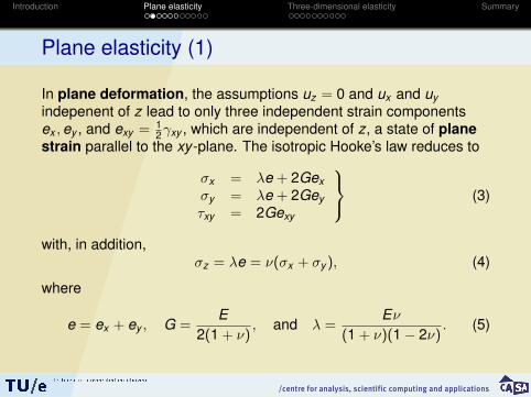
In plane deformation, the assumptions uz = 0 and ux and uyindepenent of z lead to only three independent strain componentsex ,ey , and exy = 1

2γxy , which are independent of z, a state of planestrain parallel to the xy -plane. The isotropic Hooke’s law reduces to

σx = λe + 2Gexσy = λe + 2Geyτxy = 2Gexy

(3)

with, in addition,σz = λe = ν(σx + σy ), (4)

where

e = ex + ey , G =E

2(1 + ν), and λ =

Eν(1 + ν)(1− 2ν)

. (5)



Plane elasticity (2)

To these must be added two equations of motion

∂σx∂x +

∂τxy∂y + ρbx = ρ∂2ux

∂t2

∂τxy∂x +

∂σy∂y + +ρby = ρ

∂2uy

∂t2

}(6)

and one compatibility equation

∂2ex

∂y2 +∂2ey

∂x2 = 2∂2exy

∂x∂y, (7)

if for small displacements we ignore the difference between thematerial coordinates X ,Y and the spatial coordinates x , y .



Particular solution for body forces

The linearity can also be used to construct the solution in two parts:σij = σH

ij + σPij ,eij = eH

ij + ePij .

The particular solution σPij ,e

Pij satisfies the given equations with

given body-force distributions but not the boundary conditions.The distribution σH

ij ,eHij satisfies the homogeneous differential

equations (with no body force) and suitably modified boundaryconditions.When the body force is simply the weight, say bx = 0, by = −g,then a possible particular solution is

σPy = ρgy − C, σP

x = τPxy = 0, (8)

where −C is the value of σPy at y = 0.



Airy stress function

For plane strain with no body forces, the equilibrium equations areidentically satisfied if the stresses are related to a scalar functionφ(x , y), called Airy’s stress function, by the equations

σx =∂2φ

∂y2 , σy =∂2φ

∂x2 , τxy = − ∂2φ

∂x∂y. (9)

The compatibility equation then becomes the biharmonic equation

∇21(∇2

1)φ = 0 (10)

or∇4

1φ = 0,

where ∇1 = ∂2

∂x2 + ∂2

∂y2 is the 2D Laplace operator.



Boundary conditions for Airy stress function

Airy stress function useful for boundary conditions for tractions.Since ti = σjinj , we have tx = σxnx + τxy ny and ty = τxy nx + σy ny or

tx = ∂2φ∂y2

dyds + ∂2φ

∂x∂ydxds = d

ds

(∂φ∂y

)ty = − ∂2φ

∂x∂ydyds

∂2φ∂x2

dxds = − d

ds

(∂φ∂x

).

}(11)

Hence, integrating along the boundary, we obtain ∂φ∂x = −

∫C ty ds + C1

and ∂φ∂y =

∫C txds + C2. Now we can calculate dφ

ds = ∂φ∂x

dxds + ∂φ

∂ydyds ,

dφdn = ∂φ

∂xdyds −

∂φ∂y

dxds and φ =

∫C

dφds ds + C3 at the boundary.



Outline

1 Introduction



4 Summary



Elasticity model in cylindrical coordinates

In cylindrical coordinates, we have

u = ur er + uθeθ + uz ez .

Then the displacement-gradient tensor ∇u is derived bydifferentiating the variable unit vectors er , eθ as well as thecoefficients of the three unit vectors. Small-strain components incylindrical coordinates are

Err = ∂ur∂r Eθθ = 1

r∂uθ∂θ + ur

r Ezz = ∂uz∂z

Erθ = 12

[1r

∂ur∂θ + ∂uθ

∂r −uθr

]Eθz = 1

2

(∂uθ∂z + 1

r∂uz∂θ

)Ezr = 1

2

(∂uz∂r + ∂ur

∂z

).

(12)



Plane stress equations in polar coordinates

Plane-strain components will be denotedfor

u = uer + veθ

by er = ∂u∂r eθ = 1

r∂v∂θ + u

rerθ = 1

2

( 1r

∂u∂θ + ∂v

∂r −vr

) (13)

Hooke’s law in polar coordinates

σr = λe + 2Ger σθ = λe + 2Geθ

τrθ = 2Gerθ where e = er + eθ

σz = ν(σr + σθ.

(14)



Lamé solution for cylindrical tube (1)

Consider a tube long in the z-direction, loaded by internal pressure piand external pressure po, with negligible body forces, and assumeplane deformation with radial symmetry, independent of z and θ in theplane region a ≤ r ≤ b. The Navier equations then become, withuθ = uz = 0,ur = u, simply

(λ+ 2G)ddr

[1r

ddr

(ru)

]= 0. (15)

Two integrations with respect to r then give

u = Ar +Br. (16)

In polar coordinates we get

er =∂ur

∂r= A− B

r2 eθ =ur

r= A +

Br2 erθ = 0 (17)



Lamé solution for cylindrical tube (2)Hooke’s law gives

σr = 2Aλ+ 2GA− 2GBr2

σθ = 2Aλ+ 2GA + 2GBr2

τrθ = 0 σz = 4Aν(λ+ G).

(18)

We apply the boundary conditions at r = a and r = b.

r = a −pi = 2A(λ+ G)− 2GBa2

r = b −po = 2A(λ+ G)− 2GBb2

}(19)

whence2GB = (pi−po)a2b2

b2−a2

2(λ+ G)A = pi a2−pob2

b2−a2

}(20)

so that the stress distribution is

σr = pi a2−pob2

b2−a2 − pi−pob2−a2

a2b2

r2

σθ = pi a2−pob2

b2−a2 + pi−pob2−a2

a2b2

r2

σz = 2ν(pi a2−pob2)b2−a2 τrθ = 0.

(21)



Outline

1 Introduction



4 Summary



Outline

1 Introduction



4 Summary



Direct solution of Navier equations

(λ+ G)∂e∂Xk

+ G∇2uk + ρbk = ρ∂2uk

∂t2 where e =∂uk

∂Xk.

Already in 1969, for elastostatics, with ∂2uk∂t2 = 0, the solution of such a

set of three equations in three dimensions by finite-difference orfinite-element methods is beginning to be a possibility.An advantage of direct solving the 3D problem instead of the lesscomplex 2D problem is that strains can be obtained in terms of thefirst partial derivatives of the displacement field.



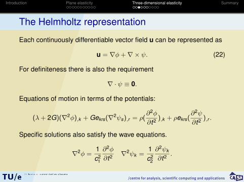
The Helmholtz representation

Each continuously differentiable vector field u can be represented as

u = ∇φ+∇× ψ. (22)

For definiteness there is also the requirement

∇ · ψ ≡ 0.

Equations of motion in terms of the potentials:

(λ+ 2G)(∇2φ),k + Gekrs(∇2ψs),r = ρ(∂2φ

∂t2 ),k + ρekrs(∂2ψ

∂t2 ),r .

Specific solutions also satisfy the wave equations.

∇2φ =1c2

1

∂2φ

∂t2 ∇2ψk =1c2

2

∂2ψk

∂t2 .



Papkovich-Neuber potentials

When the Helmholtz representation is substituted into the elastostaticNavier Eq., we get

∇2[α∇φ+∇× ψ] = −ρbG,

where α = 2(1−ν)1−2ν . The Papkovic-Neuber potentials are φ0 and Φ,

which is defined byΦ = α∇φ+∇× ψ.

Then we get Poisson’s equations{∇2Φ = −ρb

G

∇2φ0 = ρb·rG

The solution can be found by Green’s formula. In general, thepotentials satisfy complicated boundary conditions.



Green’s formula (1)

Two sufficiently differentiable functions f and g in volume V boundedby S satisfy Green’s Second Identity:∫

S

[f∂g∂n

− g∂f∂n

]dS =

∫V

[f∇2g − g∇2f

]dV . (23)

Let P be an arbitrary field point and Q a variable source point. ThenGreen’s formula expresses the value fP as follows:

4πfP =

∫S

[1r1

∂f∂n

− f∂

∂n

(1r1

)]dS −

∫V

1r1∇2fdV .



Green’s formula for the half-spaceIn potential theory the Green’s function G(P,Q) for a region is asymmetric function of the form

G(P,Q) =1r1

+ g(P,Q) ∇2g = 0.

where r1 = ‖P −Q‖. We obtain the formula for f in terms of Green’sfunction:

4πfP = −∫

Sf∂G∂n

dS −∫

VG∇2fdV .

Let Q2 be the image point of Q in the XY-plane and let r2 = ‖P −Q2‖.For the half-space, it is possible to determine G(P,Q):

G(P,Q) =1r1− 1

r2.

f (P) = − 12π

∂

∂Z

∫S

fr0

dS − 14π

∫V

G∇2fdV



Outline

1 Introduction



4 Summary



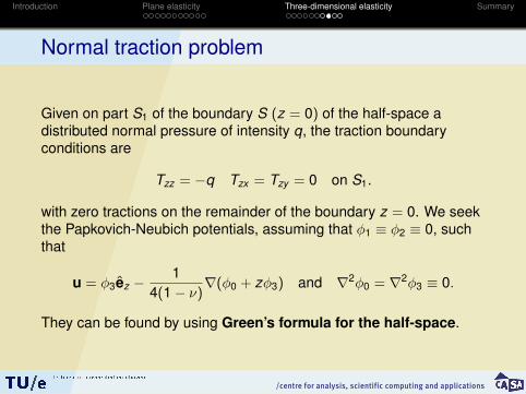
Normal traction problem

Given on part S1 of the boundary S (z = 0) of the half-space adistributed normal pressure of intensity q, the traction boundaryconditions are

Tzz = −q Tzx = Tzy = 0 on S1.

with zero tractions on the remainder of the boundary z = 0. We seekthe Papkovich-Neubich potentials, assuming that φ1 ≡ φ2 ≡ 0, suchthat

u = φ3ez −1

4(1− ν)∇(φ0 + zφ3) and ∇2φ0 = ∇2φ3 ≡ 0.

They can be found by using Green’s formula for the half-space.



Boussinesq problem of concentrated normalforce on boundary of half-space

This problem is solved by taking limit S1 → O and q →∞ such thatlimS1→O

∫S1

qdS = P, which is a finite concentrated load at O in thepositive z-direction.



Solution of Boussinesq problem

We obtainφ2(x , y , z) = (1−ν)P

πGR∂

∂Z [φ0(x , y , z)] = (1−ν)(1−2ν)PπGR

φ0(x , y , z) = (1−ν)(1−2ν)PπG log(R + z)

Now also the displacements and tractions can be computed.



Outline

1 Introduction



4 Summary



Summary

Navier’s equationsPlane elasticityAiry stress functionPlane elasticity in polar coordinatesLamé solution for tubeHelmholtz representationPapkovich-Neuber potentialsBoussinesq problem



Literature.

L.E. Malvern: Introduction to the mechanics of a continuousmedium, Prentice-Hall, 1969, pp 497-568.

Y.C. Fung: Foundations of solid mechanics, Englewood Cliffs,N.J.: Prentice-Hall, Inc., 1965.

A.E. Green, W. Zerna: Theoretical elasticity, London: OxfordUniversity Press, 1954.

A.E.H. Love: Mathematical theory of elasticity, 4th ed. New York:Dover Publications, Inc., 1944.

S. Timoshenko, J.N. Goodier: Theory of elasticity, 2nd ed. NewYork: McGraw-Hill Book Company, 1951.

H.M. Westergaard: Theory of elasticity and plasticity, New York:Dover Publications, Inc., 1952.



Literature.

L.E. Malvern: Introduction to the mechanics of a continuousmedium, Prentice-Hall, 1969, pp 497-568.

Y.C. Fung: Foundations of solid mechanics, Englewood Cliffs,N.J.: Prentice-Hall, Inc., 1965.

A.E. Green, W. Zerna: Theoretical elasticity, London: OxfordUniversity Press, 1954.

A.E.H. Love: Mathematical theory of elasticity, 4th ed. New York:Dover Publications, Inc., 1944.

S. Timoshenko, J.N. Goodier: Theory of elasticity, 2nd ed. NewYork: McGraw-Hill Book Company, 1951.

H.M. Westergaard: Theory of elasticity and plasticity, New York:Dover Publications, Inc., 1952.

Documents

Arie Verhoeven [email protected] · PDF file6 Linearized theory of elasticity Arie Verhoeven May 24 ... Airy stress function For plane strain with no body forces, the equilibrium equations