Empir Econ (2012) 43:25–54DOI 10.1007/s00181-011-0478-8

ORIGINAL PAPER

Are there different linkages of foreign capital inflowsand the current account between industrial countriesand emerging markets?

Ho-don Yan · Cheng-lang Yang

Received: 20 September 2009 / Accepted: 10 February 2011 / Published online: 27 May 2011© Springer-Verlag 2011

Abstract This article investigates the causal relationship between the currentaccount and foreign capital inflows on two groups of countries, industrial countries(ICs) and emerging markets (EMs), during the time period of 1987–2006. Apart fromincluding three sets of control variables (macroeconomic, financial, and institutional)in the regression to avoid omitted variable bias, we additionally examine whetherthere is a disparate interaction between gross capital inflows and the current accountand between net foreign inflows and the current account. Our empirical results showthat for EMs, it is mostly true that foreign capital inflow Granger causes the currentaccount, while for ICs, it is the other way around for causality although when usinggross foreign capital inflows, there is less evidence of causality detected. We also findthat for EMs, after the 1997–1998 currency crises, capital inflows change the natureof their effects on the current account, particularly for Asian EMs.

Keywords Foreign capital inflows · Current account · Financial account ·Intertemporal current account · Emerging markets · Granger causality

JEL Classification F32

H. Yan (B)Department of Economics, Feng Chia University, 100 Wen Hwa Rd., Taichung, Taiwane-mail: hdyan@fcu.edu.tw

C. YangDepartment of Managerial Economics, Nanhua University, 55 Section 1, Nanhua Rd., Zhongkeng,Dalin Township, Chiayi County, Taiwane-mail: chenglang@mail.nhu.edu.tw

123

26 H. Yan, C. Yang

1 Introduction

The resurgence of capital mobility since the end of the 1980s has led to increaseddiscussion over whether it is a curse or a blessing, in particular for emerging markets(EMs) as many were affected by currency crises during the last decade of the twentiethcentury (e.g., Eichengreen 2001; Edison et al. 2004). Those who advocate free capitalmovement argue that foreign capital flow helps countries get access to the internationalfinancial markets to facilitate investment opportunities and offers a significant increasein economic efficiency. However, an opposing view, held by Rodrik (1998) and Stiglitz(2004), among others, argues that free capital mobility does not necessarily lead toan optimal allocation of resources, as evidenced in the currency crises of the 1990swhich afflicted many EMs and were mainly initiated by massive capital inflows andthe ensuing sudden outflows precipitated the crises.1 The boom-bust foreign capitalflows that accompanied a series of currency crises in the 1990s have been dubbed a“capital account crisis (IMF 2003).2

A persistent current account deficit is a warning indicator for impending currencycrises, as indicated in Corsetti et al. (1999) and Edwards (2002). Foreign capital flowscan either spur the exuberant investment, or release the liquidity constraint to bringabout profligate consumption, therefore leading to a current account deficit, and insome extreme cases, even deviate away from the sustainable path and bring on aspeculative currency attack. The perception of a current account deficit leading to acurrency crisis has extended to the recent debate on whether the U.S. persistent currentaccount deficit, ongoing since the beginning of the 1990s, is the culprit for the currentU.S. economic debacle and the global economic meltdown (e.g., Roubini and Setser2004; Obstfeld and Rogoff 2004; McKinnon 2001; Poole 2005; Bernanke 2005).3

However, developed and developing countries are different and suggesting that theU.S. will suffer from capital account crisis that Asian countries experienced in thelate 1990s is unfitted. As opined by Caballero et al. (2005), Australia, with its flexible

1 Stiglitz (2004) argued that as there is considerable information asymmetry in international financial mar-kets, free capital mobility does not necessarily lead to an optimal allocation of resources. Rodrik (1998)emphasized that openness to international capital flows can be especially dangerous if the appropriate con-trols, regulatory apparatus, and macroeconomic frameworks are not in place. During sudden stop episodes,as indicated in Calvo (1998), foreign financing quickly dries up and sudden capital outflows deplete theforeign reserves, which deprive the central bank of the ability to defend the pegged rate regime and resultsin a currency crisis.2 Note that since 1993, the balance of payment manual provided by the IMF has reclassified most items inthe previous capital account into a newly coined account, “financial account.” Currently, the capital accountkeeps meager items, but its name usually refers to the financial account. Here, the “capital account crises”in fact indicate “financial account crises.”3 Roubini and Setser (2004) presented that once foreign investors (either private sector or central banks) stopfinancing the U.S., the “sudden stop” could spin a series of ugly adjustment, accompanied by a GDP slump.Obstfeld and Rogoff (2004) suggested that if the correction of the current account imbalance is resolved bydeep currency depreciation, then turbulent consequences are inevitable. Bernanke (2005) argued that theunprecedented low savings rate of the U.S. is due to a “global savings glut,” particularly appearing in theemerging market economies. Hence, the problem of the U.S. enduring a current account deficit does notcome from the U.S. McKinnon (2001) and Poole (2005) nonetheless pointed out that with the privilege theU.S. has under the current international dollar standard, the U.S. will not suffer from the plight of financialcrises that emerging market economies experienced in the 1990s.

123

Foreign capital inflows and the current account 27

exchange rate regime, domestic currency-denominated debt instruments, and sophisti-cated financial system, is rarely heard of suffering from an Asian-type financial crisis,even with an enduring current account deficit.4 In addition, Rodrik and Subramanian(2009) argued that financial globalization and its accompanying free capital mobilitymay be beneficial to developed countries, but it disappoints developing countries.

There has recently been a surge of research attempting to address the relationshipbetween foreign capital inflows and current account imbalances (Fry et al. 1995; Wongand Carranza 1999; Yan 2007). These studies, although using different time periodsor different sample countries, mostly conform to a general conclusion that the currentaccount Granger causes foreign capital inflows in industrial countries (ICs), while inEMs, foreign capital inflows usually cause or “push” the current account toward animbalance. The policy implication is that EMs are susceptible to the whimsical move-ment of foreign capital inflows, and therefore such countries should be cautious whenliberalizing the capital account.

Due to the important policy implication from different causal relationships of thecurrent account and foreign capital inflows between ICs and EMs, this article attemptsto further explore this issue by considering factors which were neglected from previ-ous studies. Instead of investigating an individual country, we focus on using a paneldata with two groups of countries: 23 EMs and 22 ICs. Adding three sets of controlvariables (macroeconomic, financial, and institutional) allow us to grapple with theissue of “omitted variables” bias from previous studies. In addition, ever since the1997–1998 Asian currency crises, there is a salient change in EMs in dealing with for-eign capital inflows and a current account imbalance, as noted in IMF (2007a), Ghoshet al. (2008), and Mihaljek (2008). We also investigate whether the second wave ofcapital mobility since 1997 will bring any difference in the causal relationship.

Our findings show that the current accounts of EMs are indeed susceptible to for-eign capital inflows, while the current accounts of ICs are not, although there appeardifferent implications when using net or gross foreign capital inflows. We also detectthat after 1997, foreign capital inflows have a positive causal relationship on the cur-rent account for EMs instead of the negative effect for the periods prior to 1997.This reflects the fact that EMs accumulate enormous foreign reserves in order to self-insure themselves from currency crises. In the robustness check, we use samples ofeight Asian EMs and ICs, excluding those financial centers, and achieve similar resultswhen using the full sample of countries. When using components of the current accountand foreign capital flows to examine which components serve as the driving forces ofcausality, we find that the testing results mostly remain the same, although it meritsdemonstrating which components are the driving forces for the causal relationship.

The rest of this article is organized as follows. Section 2 summarizes different the-oretical perspectives about the channels of the causal relationship between the currentaccount and financial account and reviews the relevant empirical literature. We then

4 The Australian experience of smoothly sailing through a persistent current account deficit during the1980s and the turbulent period of the Asian 1997–1998 crisis vindicates that it is groundless to worry abouta current account imbalance in the U.S. The ongoing global financial crisis, although is also proceeded withthe persistent current account deficit of the U.S. Unlike the emerging market financial crisis, it is mainlytriggered by the over-leverage and poor risk management in the banking system.

123

28 H. Yan, C. Yang

present our motivation and explain the data used in the empirical study. Section 3explains the method of panel Granger-causality estimation and the testing results,while Sect. 4 presents additional robustness tests by examining the causal relationshipusing different countries in the group and the components of the current account andforeign capital inflows. Concluding remarks are in Sect. 5.

2 Foreign capital inflows and the current account imbalance

An expedient way to show how the current account interacts with foreign capitalinflows is from the balance of payment accounting, expressed as follows:

B O P = C A + F A, (1)

where BOP, CA, and FA represent balance of payment, current account, and finan-cial account, respectively.5 FA records the net foreign capital inflows (outflows, whennegative). With a flexible exchange rate and official intervention hardly existing, BOPis close to zero and negligible. On the other hand, under a fixed or managed floatingexchange rate regime, BOP is like a residual which serves to balance the accounts ofCA and FA.

Equation 1 can be rearranged for macroeconomic analysis. CA is expressed as thedifference between national savings (S) and investment (I ), and FA is composed ofthree main components: foreign direct investment (FDI), portfolio investment (PI),and other investment (OI, mostly bank loans). In addition, the BOP accounting indi-cates that FA is the balance of foreign assets (representing gross capital outflows) andforeign liabilities (representing gross capital inflows, or FAG, which we shall discussmore later). The decomposition of CA or FA helps to catch which components are themain driving forces for the change.

Note that Eq. 1 is an accounting identity, and it does not imply any causal relation-ship. In the following, we introduce the theoretical perspectives in the related literatureto explain the possible channels of the causal relationship between the current accountand foreign capital inflows.

2.1 Theoretical perspectives on the causal channels between the current account andforeign capital inflows

The resurgence of foreign capital flows into developing countries since the end of the1980s has drawn much attention on their causes and possible consequences.6 Twofactors which operate to attract foreign capital inflows are proposed—namely, “pull”and “push” factors—as noted in Goldstein (1995) and Agènor and Montiel (1999).

5 We ignore the capital account, omitted items, and statistical error here.6 The Latin America debt crisis erupted at the beginning of the 1980s and thereafter international capitalflows were shunned from developing countries. After resolution was initiated by the Brady Plan, interna-tional capital resurged and began to flow into developing countries. See Agènor and Montiel (1999, pp.545–574).

123

Foreign capital inflows and the current account 29

“Pull” factors (also called “internal” factors) relate to those that attract capital fromabroad as a result of advantageous domestic conditions, such as a higher marginalproductivity of capital, improved creditworthiness induced by better macroeconomicpolicy, and structural reform. “Push” factors (also called “external” factors) are thosethat originate outside of the countries. For instance, unfavorable conditions in ICsresult in a low interest rate and recession, which invoke capital to flow out of ICs andinto developing countries. Calvo et al. (1993) found that external factors, not internalfactors, explain the foreign capital inflows into Latin America in the late 1980s.7

In an open economy, there is an apparent close tie between capital inflows andcurrent account. If “pull” factors are in the making for foreign capital to flow in, thenthis represents that the domestic economic environment is favorable to attract foreigninvestors, and it is plausible that the current account would lead or cause foreign cap-ital inflows. On the other hand, if it is “push” factors in the making, then this externalfactor could cause foreign capital to flow into domestic markets and cause the currentaccount to change. In reality, both pull and push effects might be at work simulta-neously and which factor dominates can only be determined empirically. Except forthese two different driving forces of capital inflows which can bring about differentcausal relationships, there are various theoretical perspectives which could explainthe rationale of the causal relationship between foreign capital inflows and the currentaccount.

2.1.1 Intertemporal model of current account

The intertemporal current account balance model, as advocated by Sachs (1981, 1982)and Obstfeld and Rogoff (1996), among others, suggests that foreign capital inflowsserve to finance the gap of national saving and investment. The current account func-tions as a “buffer stock” to smooth the intertemporal consumption. As a result, foreigncapital inflows serve a purpose to finance the current account imbalance. Foreign cap-ital inflows are attracted into the country to finance domestic investment, because ofthe host country’s rosy investment opportunity, or to finance increasing consumptiondue to a promising future as a result of high economic growth and wealth creationfrom the “New Economy.”8 This view of foreign capital inflows, serving to fill the gapcreated from the difference between savings and investment, has permeated into mostof the reasoning on the issues of a current account deficit. According to this approach,the current account leads, or causes foreign capital inflows.

7 The conclusion of Calvo et al. (1993) is based on the finding that international reserve accumulation andreal exchange rate appreciation in Latin American capital-receiving countries are highly correlated withvarious U.S. financial variables.8 Pakko (1999) argued that the U.S. current account deficit is attributable to its immense investment oppor-tunities and strong economy. Engle and Rogers (2006) showed that expected higher future income growthwill make up the gap of a current shortage on savings.

123

30 H. Yan, C. Yang

2.1.2 Country portfolio: international wealth diversification

With the ongoing global financial integration since the 1980s, countries’ holdingsof external assets have grown rapidly as shown by Lane and Milesi-Ferretti (2001,2006), and investors are allowed to reap benefits by exercising portfolio diversifica-tion as Driessen and Laeven (2007) demonstrated. Ventura (2001) and Kraay et al.(2005) proposed that the determination of the “country portfolio” can affect the currentaccount through two effects. One is the portfolio growth effect which could result fromthe change of a country’s wealth, and the other is the portfolio rebalancing effect, whichmight result from the change in the distribution of asset returns. If the deployment ofthe country portfolio governs the balance of payment accounting, then the currentaccount will passively respond to the change of the country wealth deployment. Inother words, for the purpose of diversifying a country portfolio, foreign capital inflowscan lead and drive the current account toward imbalance.

2.1.3 Summary

To summarize, with two opposing forces, whether the current account causes foreigncapital inflows or vice versa depends upon which force dominates the causality direc-tion. In general, there could be four outcomes between the current account and foreigncapital inflows. First, the current account causes, or leads, foreign capital inflows, as theintertemporal current account model implies. Second, foreign capital inflows cause, orpush, the current account imbalance, as the country portfolio model indicated . Third,there could be bi-directional causality. The principle of BOP accounting, which is anex post concept, has a tendency to bind the current account and foreign capital inflowstogether. Fourth, if domestic and foreign investors are two independent parties whomake their own investment or consumption decision, then there is no reason to expectthat there will be any causal relationship between the current account and foreigncapital inflows. This is particularly true when considering the causal relationship onthe current account with gross capital inflows, instead of net foreign capital inflows.

2.2 Extant empirical studies and this article’s motivation

To date, there are few empirical studies on the causal relationship between foreigncapital flows and the current account. Fry et al. (1995) and Wong and Carranza (1999)focused on testing the causal relationship between CA and FA for developing coun-tries.9 Sarisoy-Guerin (2003) used different causality testing methods upon 20 devel-oped countries and 19 developing countries and found that there are more developed

9 Fry et al. (1995) applied an error correction model, which assumes that CA and FA have co-movements inthe long run, and therefore the Granger non-causality can be tested. Using annual data from 1970 to 1992 fordeveloping countries, Fry et al. (1995) found 17 countries with FA Granger causing CA, 12 countries withCA Granger causing FA, and 21 countries without a causal relationship. Wong and Carranza (1999) studiedfour developing countries (Argentina, Mexico, the Philippines, and Thailand) and showed that, prior to1989 when capital mobility was restricted, there is evidence that CA Granger causes FA, while the directionof causality is the opposite from 1989Q1 to 1994Q4 when global capital mobility became prevalent.

123

Foreign capital inflows and the current account 31

countries (including the U.S.) with causality going from CA to FA, while developingcountries have more cases with causality going the opposite way.10 Yan (2007), usingseven countries each for ICs and EMs, found that it is mostly true that the financialaccount serves to finance a current account imbalance for ICs, but for the EMs thefinancial account helps push the current account toward imbalance.11 Yan argued thatdifferent causal relationships can result from disparate stages of financial develop-ment, and suggested that developing countries should be cautious while dismantlingcapital mobility.

Distinct from previous studies, there are four novelties in this empirical study.First, unlike the previous studies testing the causality within each individual country,we use a panel data with two groups of countries, namely 23 EMs and 22 ICs, todetermine a more general causal relationship between the current account and for-eign capital inflows. Second, previous studies, such as Wong and Carranza (1999)did not use control variables, while Yan (2007) only used the exchange rate andGDP as control variables. To avoid a possible omitted variable bias, we deliberatelyuse three sets of control variables: macroeconomic variables, financial variables, andinstitutional variables. Within these three groups of control variables, financial vari-ables, which emphasize the quality of financial system, has been argued as one of themain causes of global current account imbalance and international capital flows (e.g.,Dorrucci et al. 2009). Third, previous studies are mostly based on net foreign capitalinflows, which are tantamount to the financial account (FA) in the balance of paymentaccounting. In order to examine how foreign investors interact with a country’s cur-rent account, it would be more sensible to use the gross foreign capital inflows (FAG),which only include the liabilities of the financial account.12 In theory, foreign inves-tors do not consider financing a country’s current account imbalance as their purpose.Hence, it is plausible that FAG will not have any causal relationship with CA. Fourth,since the 1997–1998 Asian financial crises, there has been a significant change inthe structure of capital flows, particularly for the EMs as noted in IMF (2007b). Wealso examine whether there are different causal relationships between prior to andafter 1997.

10 Sarisoy-Guerin (2003) investigated annual data, starting variously from the 1960s up to 2000, for 20developing and 20 developed countries. Abiding by the rule of the same integrated order so as to run thecausal relation regression between CA and FA, he applied either the standard Granger-causality test orthe co-integration error correction causality test. However, pre-testing the unit root to identify the sameintegrated order reduces the number of qualified countries for the causality test to less than half.11 Using the sample period starting differently but all ending in 2003Q4, Yan (2007) also investigate thecausal relationship between current account and three different components of foreign capital inflows—for-eign direct investment (FDI), portfolio investment (PI), and other investments (OI, mainly bank loans)—andfound similar results that there is different causal relationship between EMs and ICs.12 Net foreign capital inflows are defined as the difference between foreign investors investing in thedomestic country and domestic investors investing in foreign countries. It is the result of the mixed deci-sion-making of both domestic and foreign investors. However, gross foreign capital inflows principallyrepresent only the decision-making of foreign investors.

123

32 H. Yan, C. Yang

2.3 Country samples and data

Our sample countries include 22 ICs and 23 EMs as selected in the Morgan Stan-ley Capital International (MSCI) Index.13 Since global capital mobility has resurgedfrom the end of the 1980s, our sample starts from 1987 and ends in 2006, prior to theglobal financial crisis underway since summer 2007. In Tables 1 and 2, we show thedescriptive statistics for ICs and EMs’ current account, financial account (net foreigncapital inflows, FA), and gross foreign capital inflows (FAG), which are all in termsof GDP. At the bottom of the table, the last three rows show the country mean (non-GDP weighted) of these three variables for three different time periods: 1987–2006,1987–1996, and 1997–2006.

Three features are worth noting. First, with few exceptions (Hong Kong, Singapore,and Switzerland), the temporal averages of CA and FA are moderate for most coun-tries. Even for the U.S., which has been criticized recently for its high CA deficit, theaverage CA (−2.93%) is not high. Second, for the country mean of FAG, ICs are muchhigher than EMs, or about four times higher on average, and during the second period(1997–2006) it is about seven times (ICs’ FAG reaches as high as 18.75%, while forEMs it is 2.74%).14 This indicates that ICs have much more open financial marketsand have actively diversified their assets internationally. Third, for the EMs the secondperiod exhibits that both CA and FA are in a surplus, which is in contrast to the firstperiod (1987–1996) when CA is in a deficit (−1.61%) and FA is relatively high (with2.67%). This demonstrates that after the 1997–1998 currency crises, CA has reversedto a surplus in EMs. The double-thronged flow of foreign capital from CA and FAsimply reflects dramatic increases of foreign reserves in EMs, as to self-insure fromthe devastating effects of sudden stop or currency crises (e.g., Edison 2003; Aizenmanand Lee 2006; Jeanne 2007).

Figures 1 and 2 show the scatter diagram for two pairs of variables—CA and FA,and CA and FAG—for both ICs and EMs. In Fig. 1, it is apparent that CA and FA havea negative correlation in ICs, while for the EMs, there is also a negative correlation,but it is less acute. On the contrary, in Fig. 2, CA and FAG show no correlation inICs, while for EMs it demonstrates a compellingly negative correlation. To be sure, acorrelation does not imply causality.

3 Granger-causality estimation

Based on the spirit of Granger (1969), we test the causality by investigating whetherthe lagged CA (FA) has significantly explanatory power on FA (CA). Our estimationmethodology is similar to Aizenman and Noy (2006), in which an ordinary fixed-effect

13 22 ICs include: Australia, Austria, Belgium, Canada, Denmark, Finland, France, Germany, Hong Kong,Ireland, Italy, Japan, Netherland, New Zealand, Norway, Portugal, Singapore, Spain, Sweden, Switzerland,UK, and U.S.; 23 EMs include: South Africa, Argentina, Brazil, Chile, Colombia, Egypt, Greece, India,Indonesia, Israel, Jordan, South Korea, Mexico, Morocco, Pakistan, Peru, Philippines, Sri Lanka, Taiwan,Thailand, and Turkey,14 ICs have a rather high FAG on average, even without considering those international financial centerssuch as Belgium, Hong Kong, Singapore, etc.

123

Foreign capital inflows and the current account 33

Tabl

e1

CA

,FA

,and

FAG

:ind

ustr

ialc

ount

ries

CA

(%)

FA(%

)FA

G(%

)

Cou

ntry

Mea

nM

axM

inSD

Mea

nM

axM

inSD

Mea

nM

axM

inSD

Aus

tral

ia−4

.15

−1.8

6−5

.94

0.01

14.

526.

761.

700.

015

8.28

17.4

34.

230.

031

Aus

tria

−0.7

72.

88−3

.25

0.01

50.

814.

25−3

.15

0.01

711

.64

28.7

82.

160.

089

Bel

gium

3.86

5.74

1.84

0.01

4−3

.85

−0.2

5−6

.26

0.01

956

.48

156.

294.

450.

464

Can

ada

−0.0

53.

20− 3

.09

0.02

20.

283.

82−2

.88

0.02

26.

1210

.65

2.52

0.02

0D

enm

ark

1.38

3.88

−2.8

50.

019

−0.7

36.

39−4

.86

0.03

19.

8431

.45

−8.1

00.

087

Finl

and

2.70

10.3

7−5

.57

0.05

3−2

.39

7.95

−10.

460.

058

10.1

933

.02

−0.5

90.

071

Fran

ce0.

643.

24−1

.27

0.01

3− 0

.62

2.02

−3.3

40.

013

11.0

631

.43

1.70

0.08

4G

erm

any

1.17

5.17

−1.5

10.

085

−1.1

42.

96−5

.75

0.02

68.

5719

.57

2.00

0.04

9H

ong

Kon

g6.

7511

.02

0.08

0.03

7−4

.98

2.72

−10.

250.

045

12.0

563

.07

−83.

950.

456

Irel

and

2.53

10.9

4−6

.33

0.05

1−1

.68

6.91

−19.

250.

063

71.9

619

0.85

3.61

0.65

3It

aly

−0.0

83.

18−2

.43

0.01

70.

162.

67−3

.60

0.01

86.

9915

.30

1.69

0.03

8Ja

pan

2.60

3.80

1.35

0.00

7−1

.68

1.30

−3.0

60.

011

1.65

5.92

−2.8

80.

022

Net

herl

and

4.04

7.91

1.65

0.08

2−3

.95

−0.0

3−7

.79

0.02

421

.47

45.7

82.

950.

147

New

Zea

land

−4.5

2−1

.80

−9.0

50.

022

4.11

13.0

5−2

.26

0.03

66.

2715

.56

−4.5

80.

042

Nor

way

6.55

16.4

1−4

.44

0.06

5−5

.65

4.20

−17.

510.

064

9.47

36.8

0−2

.47

0.09

5Po

rtug

al−3

.73

1.03

−8.9

70.

035

4.67

9.70

−3.6

80.

036

14.8

330

.33

1.82

0.08

3Si

ngap

ore

14.5

927

.32

−0.7

70.

068

−6.4

56.

32−1

8.32

0.07

724

.88

56.7

0−1

.94

0.13

1Sp

ain

−2.1

90.

99−8

.01

0.02

32.

388.

05−2

.30

0.02

812

.16

25.6

00.

140.

074

Swed

en1.

927.

50−3

.36

0.03

4−1

.58

6.01

−7.2

40.

042

11.7

427

.17

2.12

0.07

6Sw

itzer

land

8.64

14.7

12 .

570.

037

−8.0

9−1

.72

−18.

450.

045

16.8

355

.45

1.33

0.14

3U

K−1

.99

0.01

−5.0

50.

012

2.11

4.73

−0.3

10.

014

26.3

961

.08

4.50

0.16

0U

.S.

−2.9

3−0

.03

−6.1

80.

018

2.94

6.16

−0.0

70.

017

6.71

14.0

91.

850.

033

Cou

ntry

mea

n(u

nwei

ghte

d)19

87–2

006

1.12

−0.3

712

.72

1987

–199

60.

560.

409.

0519

97–2

006

2.03

−1. 6

318

.75

Not

e:A

llth

eda

taar

efr

omIF

S.C

A,F

A,a

ndFA

Gre

pres

entt

hecu

rren

tacc

ount

,net

fore

ign

capi

tali

nflow

s,an

dgr

oss

fore

ign

capi

tali

nflow

s,re

spec

tivel

y.A

llar

ein

term

sof

GD

P.C

ount

rym

ean

isca

lcul

ated

byus

ing

non-

GD

Pw

eigh

t

123

34 H. Yan, C. Yang

Tabl

e2

CA

,FA

,and

FAG

:em

ergi

ngm

arke

ts

CA

(%)

FA(%

)FA

G(%

)

Cou

ntry

Mea

nM

axM

inSD

Mea

nM

axM

inSD

Mea

nM

axM

inSD

Sout

hA

fric

a−0

.62

7.47

−11.

800.

036

0.49

12.0

8−6

.85

0.03

20.

030.

54−0

.62

0.00

2A

rgen

tina

−0.5

98.

94−4

.82

0.03

8−0

.63

8.89

−19.

870.

072

1.46

11.8

3−1

2.63

0.07

0B

razi

l−0

.95

1.82

−4.2

70.

021

0.78

4.95

−3.5

80.

024

1.87

5.67

−3.1

20.

025

Chi

le−1

.60

3.61

−5.3

60.

023

2.57

9.26

−4.2

80.

043

7.05

16.3

9−5

.21

0.05

3C

olom

bia

−1.3

94.

78−5

.39

0.02

72.

276.

56−1

.19

0.02

23.

888.

93−0

.47

0.02

9E

gypt

1.11

6.75

−3.0

30.

029

−2.7

63.

375.

620.

056

−0.2

19.

57−1

8.99

0.05

8G

reec

e− 3

.81

−0.1

5−9

.59

0.02

34.

429.

690.

250.

024

6.99

19.8

5−0

.63

0.05

5In

dia

−0.9

41.

48−2

.36

0.01

02.

333.

741.

320.

006

2.52

5.22

1.09

0.01

0In

done

sia

0.17

4.84

−3.3

70.

030

0.39

5.35

−7.8

90.

034

1.03

5.37

−10.

050.

041

Isra

el−0

.24

6.26

−4. 2

80.

026

−0.3

88.

83−1

3.02

0.04

83.

9414

.29

−11.

790.

047

Jord

an−2

.47

13.1

3−1

7.60

0.08

27.

1155

.67

−7.9

80.

140

7.90

35.6

6−1

7.38

0.12

0So

uth

Kor

ea1.

6311

.74

−4.2

70.

039

0.72

4.52

−5.7

30.

026

2.95

8.68

−6.1

50.

035

Mal

aysi

a4.

0417

.11

−9.7

30.

090

0.58

21.5

7−1

2.51

0.09

34.

7517

.55

−3.0

70.

055

Mex

ico

−2.4

83.

03−7

.05

0.02

32.

947.

60−5

.15

0.03

33.

809.

27−1

.50

0.02

7M

oroc

co0.

194.

71−3

.94

0.02

40.

277.

35−4

.21

0.03

10.

778.

35−3

.62

0.03

2Pa

kist

an−2

.32

5.64

−7.5

50.

035

2.35

7.02

− 3.6

00.

032

2.54

7.63

−3.7

50.

036

Peru

−3.7

72.

64−8

.57

0.02

82.

699.

60−5

.13

0.04

24.

0610

.00

0.68

0.02

9Ph

ilipp

ines

−1.8

05.

13−6

.08

0.03

03.

1710

.01

−2.2

50.

035

4.92

15.7

0−0

.65

0.04

1Sr

iLan

ka−3

.74

−0.1

7−6

.61

0.01

93.

9011

.13

−1. 8

20.

037

3.52

8.49

−2.2

20.

035

Taiw

an5.

5017

.32

1.18

0.03

7−1

.33

9.71

−9.1

90.

045

5.38

14.5

1−0

.91

0.04

2T

haila

nd−0

.84

12.7

3−8

.53

0.06

32.

8612

.41

−15.

140.

084

4.09

15.2

0−9

.47

0.07

6T

urke

y−1

.61

2.33

−8.1

20.

028

2.45

12.6

2−1

1.18

0.04

83.

6515

.66

−8.7

00.

053

Ven

ezue

la4.

0417

.04

−9.6

20.

076

−3.2

55.

11−1

2.95

0.05

42.

347.

96−7

.22

0.03

8C

ount

rym

ean

(unw

eigh

ted)

1987

–200

6−0

.94

1.77

3.18

1987

–199

6−1

.61

2.67

3.45

1997

–200

60.

170.

282.

74

Not

e:A

llth

eda

taar

efr

omIF

S.C

A,F

A,a

ndFA

Gre

pres

entt

hecu

rren

tacc

ount

,net

fore

ign

capi

tali

nflow

s,an

dgr

oss

fore

ign

capi

tali

nflow

s,re

spec

tivel

y.A

llar

ein

term

sof

GD

P.C

ount

rym

ean

isca

lcul

ated

byus

ing

non-

GD

Pw

eigh

t

123

Foreign capital inflows and the current account 35

Emerging Markets

-0.4

-0.2

0

0.2

0.4

0.6

-0.2 -0.1 0 0.1 0.2

CA

FA

Industrial Countries

-0.3

-0.2

-0.1

0

0.1

0.2

-0.2 -0.1 0 0.1 0.2 0.3

CA

FA

Fig. 1 Scatter diagram for CA and FA

model of panel estimation was implemented. While Aizenman and Noy (2006) focusedon the causality between trade openness and financial openness, we are interested inthe causality between a current account imbalance and foreign capital inflows.15

3.1 Panel causality estimation

The panel estimation equations are shown as follows.

C Ait = aC Ai + bC A

1 F Ait−1 + bC AD (Dit−1 × F Ait−1) + bC A

2 C Ait−1 + bC A3 Mit

+bC A4 Fit + bC A

5 Ii t + eit (2a)

F Ait = aF Ai + bF A

1 C Ait−1 + bF AD (Dit−1 × C Ait−1) + bF A

2 F Ait−1 + bF A3 Mit

+bF A4 Fit + bF A

5 Ii t + eit , (2b)

15 Our testing methodology is similar to Aizenman and Noy (2006) with two main differences. The first isabout the purpose. Aizenman and Noy (2006) emphasized on whether trade openness or financial opennessleads, while we are interested in the relationship between the current account and foreign capital inflows.Aizenman and Noy (2006) focused on the causal relationship between FDI and current account imbalance(exports and imports), while we focus on the relationship between CA (S and I ) and foreign capital inflows.Second, in the panel causality test we add a dummy interaction term to capture whether there is a disparityin the causal relationship between the current account and foreign capital inflows prior to and after the1997–1998 Asian currency crises.

123

36 H. Yan, C. Yang

Industrial Countries

-1

0

1

2

3

-0.2 -0.1 0 0.1 0.2 0.3

CA

FAG

Emerging Markets

-0.4

-0.2

0

0.2

0.4

-0.2 -0.1 0 0.1 0.2

CA

FAG 1

Fig. 2 Scatter diagram for CA and FAG

where CA and FA represent the current account and net capital inflows (or financialaccount). The estimated coefficients are denoted with a superscript align with thedependent variable. Term ai is the country fixed effect, which is used to control forunobservable heterogeneity, and Dit is a dummy variable and it is 0 for the time periodof 1987–1996, while it equals 1 for 1997–2006.

As suggested by IMF (2007a), after the 1997–1998 Asian financial crises therehas been another wave of foreign capital inflows and a reversal of the current accounttoward a surplus in EMs, and this might influence the causal relationship. We thereforeadd a dummy interaction term to examine whether there is a different causal relation-ship. The null hypothesis of no-Granger-causality tests whether the estimated coef-ficients of the lagged variable, C Ait−1(F Ait−1), and the lagged dummy interactionterm, Dit−1 × C Ait−1 (Dit−1 × F Ait−1), i.e., bC A

1 (bF A1 ) and bC A

D (bF AD ), are signif-

icantly different from zero. In order to have parsimonious estimated coefficients, thelag (t −1) used here represents the one lag average over four periods, t −1, . . . , t −4.16

16 Using one lag average over four lagged periods allows us to capture the causal relationship by estimatinga parsimonious regression and to save the degree of freedom. See the similar application in Aizenman andNoy (2006). We also consider two other ways to specify lags used in the regression for testing Grangercausality. First, instead of using one lag average over four lags, we can directly use four different lags inthe regression. Second, except using the one lag average over four lagged periods on the causal variables,we can extend the one lag average over four lagged periods to the control variables. We exercised these twodifferent lag specifications and we found that the causal relationship mostly remain the same. The resultsare available from the authors upon request.

123

Foreign capital inflows and the current account 37

3.2 Control variables

In the spirit of the Granger-causality test, we include the lagged dependent variableas one of the regressors, and the other control variables included seek to capturethose factors which could cause foreign capital inflows (e.g., Goldstein 1995; Agènorand Montiel 1999) and the current account (e.g., Chinn and Prasad 2003; Chinn andIto 2007). We categorize control variables into three groups: macroeconomic vari-ables (M), financial variables (F), and institutional variables (I ). The description andsources of those control variables can be seen in the appendix.

Macroeconomic control variables include GDP (YX, growth rate of GDP), exchangerate (EX, growth rate of exchange rate), and economic openness (OPEN). Except fortwo control variables, YX and EX used in Yan (2007), we add the scale of an econ-omy’s openness, which could affect the current account and foreign capital inflows, asargued by Chinn and Prasad (2003) and Aizenman and Noy (2006). However, whethereconomic openness will bring a positive or negative influence on CA and FA (FAG)can only be determined empirically.17

Financial variables include financial deepness (the ratio of private credit by depositmoney banks and other financial institutions over GDP; Beck et al. 2000), the financialdevelopment (ratio of the value of total shares traded to average real market capitali-zation, SMTV; Beck et al. 2000), and financial account openness (KAOP; Chinn andIto 2008).18 Financial deepness strengthens the capacity of a country to absorb largeinflows or outflows of foreign capital and it could increase the saving rate and affectthe current account, although its effect on CA and FA (FAG) is ambiguous. Financialdevelopment may lead to higher savings and therefore CA surplus (Chinn and Ito2007), but it could be beneficial for investment. Therefore, whether it will cause apositive or negative effect on CA is uncertain. Likewise, there is no definite answerthat financial development will bring more capital inflows or outflows, and therefore anegative or positive FA. Whether financial openness is beneficial or detrimental to aneconomy has been a hotly debated issue (Prasad et al. 2007). Financial openness influ-ences CA and FA, but whether its effect on the current account and financial accountis negative or positive remains an empirical question.

17 We also add a dependence ratio (ratio of the number of people aged below 14 plus those aged above 64over those aged between the ages of 15 and 65), and a government budget deficit. Both cannot change thefundamental casual relationship and for brevity we do not present the estimated results of including thesetwo variables.18 We also tried the ratio of M2 over GDP as an indicator for financial deepness, and the estimations aremostly insignificant and irrelevant for the determination of causality. In Beck et al. (2000), there are othertwo measures of financial development including the stock market capitalization ratio and stock markettotal value traded (in terms of GDP), for brevity we do not present their estimation results. KAOP is basedon IMF’s Annual Report on Exchange Arrangements and Restrictions, in which four major categories ofvariables on the restrictions of external accounts are adopted: presence of multiple exchange rates, restric-tions on current account transactions, restrictions on capital account restriction, and the requirements ofthe surrender of export proceeds. The index of KAOP is calculated from the first standardized principalcomponent of these four variables. With duly adjustment, the index takes a higher value the more open thecountry is to cross-broader capital transaction.

123

38 H. Yan, C. Yang

Institutional variables include the index of corruption (CU), political stability (ST),and law and order (LA).19 An economy with high corruption will be less attractive toforeign capitals, but its effect on the current account could be undetermined due tothe negative effect on both savings and investment. A stable political system certainlyattracts more foreign capital, but whether it will bring a positive or negative effecton the current account is indeterminate. A country following the law and order isapt to elicit more foreign investors, and in the meantime, it allows domestic inves-tors to allocate their assets in foreign countries. Therefore, we are unable to ascertainwhether it has positive or negative effects on foreign capital inflows and the currentaccount.

The correlation coefficients show scant evidence of multi-collinearity among cur-rent account (and its components, S and I ), foreign capital inflows (both net andgross, FA and FAG; and their components, FDI and FDIG, PI and PIG, and OI, andOIG) and all related control variables.20 To assure that all the variables included inthe regression follow the stationary process, those causal variables, macroeconomicvariables and financial variables are either expressed in terms of GDP (such as CA, FA,FAG, and their components), or in the change rate (such as YX, EX). For institutionalvariables, since they change in a glacial pace, they are relatively stable. To be sure, wealso implemented variant panel unit root tests for each variable to avoid the possiblespurious regression.21

3.3 Causality between the current account and foreign capital inflows

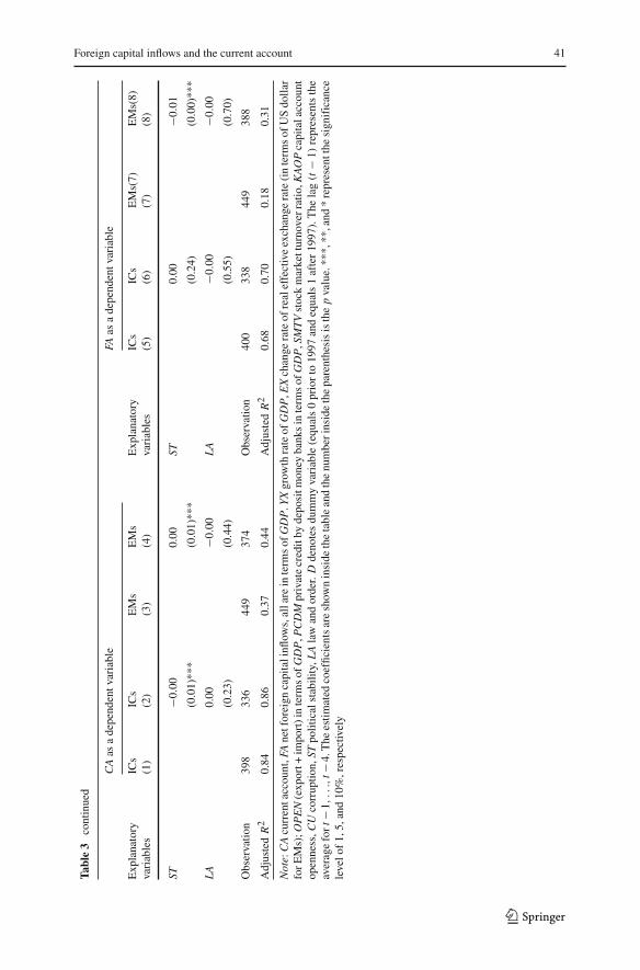
In order to show whether there is biased from omitted variable, we present estimationresults without and with control variables.22 We use the ordinary OLS estimation ofthe fixed-effect model with panel corrected standard errors following the suggestionof Beck and Katz (1995). This estimator allows for cross-sectional heteroskedasticityand contemporaneous correlation of the residuals.23 Table 3 are the estimation resultsfor the cases of using CA and net foreign capital inflows (FA) as dependent variables,and Table 4 are the results for the cases of causal estimations between CA and gross

19 These three indices are from International Country Risk Guide (ICRG). Corruption is an index with arange from 0 to 6, whereby the higher the index, the less corruption, and vice versa. Political stability is anindex which has a range from 0 to 12, and the higher the index, the better the political stability. Law andorder has an index ranging from 0 to 6, and the higher the index, the better is a country’s law and order.20 For brevity, we do not present the correlation coefficients. They are available from the authors uponrequest.21 We use four different panel unit root tests and the regression model used includes individual constantterm and the AIC is used to select the lags. Most variables can reject the null hypothesis of panel unitroot, although some variables can be rejected only under other identifications of the model, such as withindividual constant term and trend term. Results of panel unit root tests are available from the authors uponrequest.22 There are only 22 EMs included when control variables are added because Taiwan is excluded for lackof available data of three financial control variables.23 We use another method of White-type standard errors for the system of equations, which will producethe estimator robust to a cross-equation correlation as well as different error variance in cross-section(Wooldridge 2002; Arellano 1987). The causal results remain the same.

123

Foreign capital inflows and the current account 39

capital inflows (FAG). As shown in both tables, the adjusted R2 is higher for ICs thanfor EMs and for CA than FA as a dependent variable. For instance, Table 3 showsthat for the case with control variables, when using CA as the dependent variable, theadjusted R2 is around 0.86 for ICs and around 0.44 for EMs. On the other hand, whenusing FA as the dependent variable, the adjusted R2 is around 0.68 for ICs and 0.31for EMs. In addition, adding control variables apparently brings higher adjusted R2.

3.3.1 Using net capital inflows

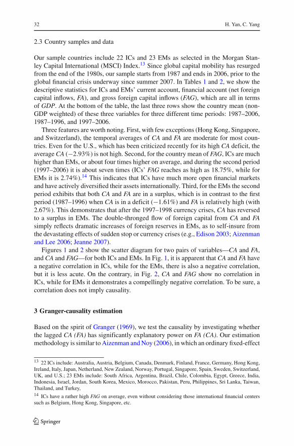
Columns (1)–(4) of Table 3 present the estimated results of using CA as the dependentvariable. Whether foreign capital inflows will affect CA depends upon the estimatedcoefficients of the first two rows: F At−1 and Dt−1 × F At−1. For ICs, as shown incolumns (1)–(2) the estimated coefficient of lagged FA (i.e., F At−1) and the dummyintersection term with lagged FA (i.e., Dt−1 × F At−1) are insignificant. This indi-cates that for ICs, FA does not Granger-cause CA. For the cases of EMs, as shown incolumns (3)–(4), the estimated coefficients of F At−1 are significant either without orwith control variables (−0.44 and −0.51, respectively). The estimated coefficient ofthe dummy intersection term, Dt−1 × F At−1, is significant when control variables arenot included, but it turns insignificant when adding control variables. It is interestingto note that the estimated coefficients of Dt−1 × F At−1 are all positive, and this isdifferent from the negative estimated coefficient of F At−1. This result suggests thatfor EMs, after 1997 there is a change in the nature of capital inflows affecting CAalthough the marginal effect in the second period remains negatively signed as in thefirst period.

Columns (5)–(8) present the results of using FA as the dependent variable. ForICs, whether using control variables or not, the lagged variable C At−1 is significantalthough only under the 10% significance level, and the estimated coefficients of thedummy intersection term, Dt−1 × C At−1, is also significant although under the 10%significance level (the model without using control variables is significant under the5% significance level). There is evidence of Granger causality going from CA to FAfor ICs although it is rather weak. For EMs, the estimated coefficients of C At−1 areinsignificant either adding control variables or not. However, the estimated coefficientsof Dt−1 × C At−1 are significant (under the 10% significance level) without addingcontrol variables, but when adding control variables it turns insignificant.

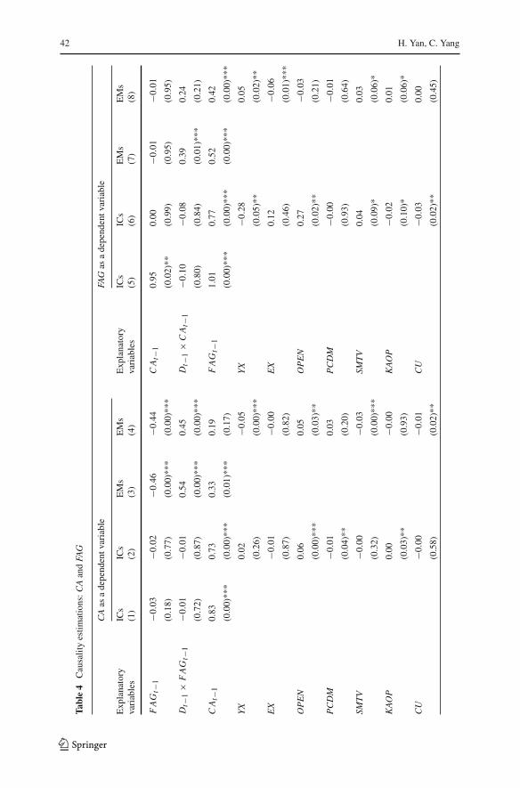
3.3.2 Using gross capital inflows

When implementing the estimation by using gross foreign capital inflows, we simplyreplace FA in Eqs. 2a and 2b with FAG. Columns (1)–(2) of Table 4 show that forICs, no causality from FAG to CA is detected, whether control variables are includedor not. On the contrary, for EMs, as shown in columns (3)–(4), the causality goingfrom FAG to CA is rather conspicuous. It is worth noting that the estimated coeffi-cient of F AGt−1 is negative, but the estimated coefficient of the dummy intersectionterm, Dt−1 × F AGt−1, turns out to be a dominant positive. As shown in column(4), the estimated coefficient of F AGt−1 is −0.44, while the estimated coefficientof Dt−1 × F AGt−1 is 0.45, which indicates that in the second period, FAG Granger

123

40 H. Yan, C. Yang

Tabl

e3

Cau

salit

yes

timat

ions

:CA

and

FA

CA

asa

depe

nden

tvar

iabl

eFA

asa

depe

nden

tvar

iabl

e

Exp

lana

tory

ICs

ICs

EM

sE

Ms

Exp

lana

tory

ICs

ICs

EM

s(7)

EM

s(8)

vari

able

s(1

)(2

)(3

)(4

)va

riab

les

(5)

(6)

(7)

(8)

FA

t−1

−0.1

6−0

.19

−0.4

4−0

.51

CA

t−1

−0.3

2−0

.38

−0.1

10.

16

(0.2

6)(0

.21)

(0.0

0)**

*(0

.00)

***

(0.1

1)(0

.07)

*(0

.58)

(0.5

8)

Dt−

1×

FA

t−1

−0.1

50.

070.

260.

18D

t−1C

At−

1−0

.25

−0.2

40.

330.

02

(0.1

4)(0

.54)

(0.0

7)*

(0.1

6)(0

.04)

**(0

.06)

*(0

.08)

*(0

.94)

CA

t−1

0.55

0.63

0.23

−0.0

5F

At−

10.

280.

160.

410.

41

(0.0

0)**

*(0

.00)

***

(0.0

9)*

(0.7

1)(0

.18)

(0.4

9)(0

.01)

***

(0.0

3)**

YX

0.01

−0.0

3Y

X0.

000.

06

(0.4

4)(0

.00)

***

(0.9

5)(0

.00)

***

EX

−0.0

00.

01E

X0.

03−0

.06

(0.9

9)(0

.56)

(0.4

2)(0

.01)

***

OP

EN

0.06

0.04

OP

EN

−0.0

0−0

.04

(0.0

0)**

*(0

.06)

*(0

.86)

(0.2

5)

PC

DM

−0.0

10.

04P

CD

M−0

.00

−0.0

3

(0.0

1)**

*(0

.12)

(0.6

9)(0

.24)

SMT

V−0

.01

−0.0

3SM

TV

−0.0

00.

05

(0.1

4)(0

.00)

***

(0.9

7)(0

.00)

***

KA

OP

0.00

0.00

KA

OP

−0.0

10.

00

(0.1

5)(0

.46)

(0.0

0)**

*(0

.66)

CU

−0.0

0−0

.00

CU

−0.0

00.

01

(0.8

8)(0

.00)

***

(0.3

8)(0

.18)

123

Foreign capital inflows and the current account 41

Tabl

e3

cont

inue

d

CA

asa

depe

nden

tvar

iabl

eFA

asa

depe

nden

tvar

iabl

e

Exp

lana

tory

ICs

ICs

EM

sE

Ms

Exp

lana

tory

ICs

ICs

EM

s(7)

EM

s(8)

vari

able

s(1

)(2

)(3

)(4

)va

riab

les

(5)

(6)

(7)

(8)

ST−0

.00

0.00

ST0.

00−0

.01

(0.0

1)**

*(0

.01)

***

(0.2

4)(0

.00)

***

LA

0.00

−0.0

0L

A−0

.00

−0.0

0

(0.2

3)(0

.44)

(0.5

5)(0

.70)

Obs

erva

tion

398

336

449

374

Obs

erva

tion

400

338

449

388

Adj

uste

dR

20.

840.

860.

370.

44A

djus

ted

R2

0.68

0.70

0.18

0.31

Not

e:C

Acu

rren

tacc

ount

,FA

netf

orei

gnca

pita

linfl

ows,

alla

rein

term

sof

GD

P.Y

Xgr

owth

rate

ofG

DP

,EX

chan

gera

teof

real

effe

ctiv

eex

chan

gera

te(i

nte

rms

ofU

Sdo

llar

forE

Ms)

;OP

EN

(exp

ort+

impo

rt)i

nte

rms

ofG

DP

,PC

DM

priv

ate

cred

itby

depo

sitm

oney

bank

sin

term

sof

GD

P,S

MT

Vst

ock

mar

kett

urno

verr

atio

,KA

OP

capi

tala

ccou

ntop

enne

ss,C

Uco

rrup

tion,

STpo

litic

alst

abili

ty,L

Ala

wan

dor

der.

Dde

note

sdu

mm

yva

riab

le(e

qual

s0

prio

rto

1997

and

equa

ls1

afte

r19

97).

The

lag

(t−

1)re

pres

ents

the

aver

age

fort

−1,..

.,t−

4.T

hees

timat

edco

effic

ient

sar

esh

own

insi

deth

eta

ble

and

the

num

beri

nsid

eth

epa

rent

hesi

sis

the

pva

lue.

***,

**,a

nd*

repr

esen

tthe

sign

ific

ance

leve

lof

1,5,

and

10%

,res

pect

ivel

y

123

42 H. Yan, C. Yang

Tabl

e4

Cau

salit

yes

timat

ions

:CA

and

FAG

CA

asa

depe

nden

tvar

iabl

eFA

Gas

ade

pend

entv

aria

ble

Exp

lana

tory

ICs

ICs

EM

sE

Ms

Exp

lana

tory

ICs

ICs

EM

sE

Ms

vari

able

s(1

)(2

)(3

)(4

)va

riab

les

(5)

(6)

(7)

(8)

FA

Gt−

1−0

.03

−0.0

2−0

.46

−0.4

4C

At−

10.

950.

00−0

.01

−0.0

1

(0.1

8)(0

.77)

(0.0

0)**

*(0

.00)

***

(0.0

2)**

(0.9

9)(0

.95)

(0.9

5)

Dt−

1×

FA

Gt−

1−0

.01

−0.0

10.

540.

45D

t−1

×C

At−

1−0

.10

−0.0

80.

390.

24

(0.7

2)(0

.87)

(0.0

0)**

*(0

.00)

***

(0.8

0)(0

.84)

(0.0

1)**

*(0

.21)

CA

t−1

0.83

0.73

0.33

0.19

FA

Gt−

11.

010.

770.

520.

42

(0.0

0)**

*(0

.00)

***

(0.0

1)**

*(0

.17)

(0.0

0)**

*(0

.00)

***

(0.0

0)**

*(0

.00)

***

YX

0.02

−0.0

5Y

X−0

.28

0.05

(0.2

6)(0

.00)

***

(0.0

5)**

(0.0

2)**

EX

−0.0

1−0

.00

EX

0.12

−0.0

6

(0.8

7)(0

.82)

(0.4

6)(0

.01)

***

OP

EN

0.06

0.05

OP

EN

0.27

−0.0

3

(0.0

0)**

*(0

.03)

**(0

.02)

**(0

.21)

PC

DM

−0.0

10.

03P

CD

M−0

.00

−0.0

1

(0.0

4)**

(0.2

0)(0

.93)

(0.6

4)

SMT

V−0

.00

−0.0

3SM

TV

0.04

0.03

(0.3

2)(0

.00)

***

(0.0

9)*

(0.0

6)*

KA

OP

0.00

−0.0

0K

AO

P−0

.02

0.01

(0.0

3)**

(0.9

3)(0

.10)

*(0

.06)

*

CU

−0.0

0−0

.01

CU

−0.0

30.

00

(0.5

8)(0

.02)

**(0

.02)

**(0

.45)

123

Foreign capital inflows and the current account 43

Tabl

e4

cont

inue

d

CA

asa

depe

nden

tvar

iabl

eFA

Gas

ade

pend

entv

aria

ble

Exp

lana

tory

ICs

ICs

EM

sE

Ms

Exp

lana

tory

ICs

ICs

EM

sE

Ms

vari

able

s(1

)(2

)(3

)(4

)va

riab

les

(5)

(6)

(7)

(8)

ST−0

.00

0.00

ST0.

00−0

.02

(0.0

7)*

(0.2

6)(0

.98)

(0.0

7)*

LA

0.01

−0.0

0L

A−0

.01

−0.0

0

(0.0

7)*

(0.6

9)(0

.39)

(0.2

7)

Obs

erva

tion

398

326

434

375

Obs

erva

tion

400

328

433

374

Adj

uste

dR

20.

840.

860.

400.

43A

djus

ted

R2

0.75

0.81

0.21

0.31

Not

e:C

Acu

rren

tac

coun

t,FA

Ggr

oss

fore

ign

capi

tal

inflo

ws,

all

are

inte

rms

ofG

DP

.YX

grow

thra

teof

GD

P,E

Xch

ange

rate

ofre

alef

fect

ive

exch

ange

rate

(in

term

sof

US

dolla

rfo

rE

Ms)

;O

PE

N(e

xpor

t+

impo

rt)

inte

rms

ofG

DP

,PC

DM

priv

ate

cred

itby

depo

sit

mon

eyba

nks

inte

rms

ofG

DP

,SM

TV

stoc

km

arke

ttu

rnov

erra

tio,K

AO

Pca

pita

lacc

ount

open

ness

,CU

corr

uptio

n,ST

polit

ical

stab

ility

,LA

law

and

orde

r.D

deno

tes

dum

my

vari

able

(equ

als

0pr

ior

to19

97an

deq

uals

1af

ter

1997

).T

hela

g(t

−1)

repr

esen

tsth

eav

erag

efo

rt−

1,..

.,t−

4.T

hees

timat

edco

effic

ient

sar

esh

own

insi

deth

eta

ble

and

the

num

ber

insi

deth

epa

rent

hesi

sis

the

pva

lue.

***,

**,a

nd*

repr

esen

tth

esi

gnif

ican

cele

velo

f1,

5,an

d10

%,r

espe

ctiv

ely

123

44 H. Yan, C. Yang

causes CA with a positive marginal effect of 0.01. For EMs, as compared to column(4) of Table 3 when FA is used, the second period of FAG does play a disparate andstronger role to cause CA.

Columns (5)–(8) of Table 4 show the estimation results when FAG serves as thedependent variable. For ICs, while no control variables added, the estimated coeffi-cient of F AGt−1 is significant, as shown in column (5). However, column (6) showsthat when adding control variables, no causal relationship is detected for ICs underthe 5% significance level. For EMs, the estimated coefficients of C At−1 are all insig-nificant either adding control variables or not. Although the estimated coefficient ofdummy intersection term Dt−1 × C At−1 is significant, as shown in column (7), itturns insignificant after adding control variables, as shown in column (8).

3.3.3 Summary

We find that adding control variables make a difference for the causal relationship. Thisdifference is more acute for the cases between CA and FAG. For both ICs and EMs,without adding control variables, it is evident that there is Granger causality goingfrom CA to FAG, while after adding control variables, the causal relationship disap-pears. Based on the evidence from models of using control variables, there is Grangercausality going from CA to FA for ICs, while for EMs, it is the other way around thatFA Granger causes CA. This is similar to what found in Sarisoy-Guerin (2003) and Yan(2007). However, we also found that there is almost no causal relationship detectedbetween CA and FAG for ICs. It indicates that there exists a decoupled decision-makingbetween foreign investors and domestic agents. Indeed, with a sophisticated financialsystem in ICs, there is no reason to expect that domestic investors and foreign investorswill have any connection when making their investment decisions. For EMs, althoughthere is evident that gross foreign capital inflows serve to push CA toward imbalances,we also found that in the second period FA and FAG change the nature of its influenceon CA. This resonates what IMF (2007b) observed that two waves (prior to and afterthe 1997–1998 crises) of international capital movement to EMs exhibited differentfeatures.

4 Additional robustness check

Considering that the foregoing estimation results might be contaminated when usingdifferent country samples, we group eight Asian EMs (EMs-8) and exclude sevenfinancial centers and Ireland from ICs (ICs-14) to test whether the causal relation-ship will be different.24 In addition, there might be aggregation bias because CA andFA (FAG) are aggregated variables. Hence, the causal relationship might exist, but it

24 Asian EMs include eight countries: India, Indonesia, South Korea, Malaysia, Pakistan, the Philippines,Sri Lanka, and Thailand. Taiwan is not included due to the available data of financial variables. ICs-14,after excluding seven financial centers (Belgium, Hong Kong, the Netherlands, Singapore, Switzerland,UK, and the U.S.) and Ireland, contain 14 countries: Australia, Austria, Canada, Denmark, Finland, France,Germany, Italy, Japan, New Zealand, Norway, Portugal, Spain, and Sweden. Ireland is not included becauseof its high and unusual capital inflows ratio, particularly the gross capital inflows as shown in Table 1.

123

Foreign capital inflows and the current account 45

might be canceled out due to an opposite causal relationship in their components. Forinstance, CA is the difference between national saving (S) and investment (I ), andforeign capital inflows might affect S or I , but their effect might be obscure when usingCA instead. On the other hand, FA(FAG) is composed of three components: foreigndirect investment, FDI (FDIG), portfolio investment, PI (PIG), and other investment,OI (OIG). With different natures of these three components, each could have a dispa-rate relationship withCA. As noted, FDI is usually for the long-term purpose and isrelatively more stable, while OI (consisting mainly of short-term bank loans) and PIare rather whimsical, as witnessed during the Asian currency crises (Sarno and Taylor1999a; Baily et al. 2000; Sula and Willet 2009).25

4.1 Using different country groups

In Table 5, columns (1) and (2) are the estimated results for testing whether FA Grangercauses CA, and columns (3) and (4) show estimated results of the other way around,i.e., whether CA Granger causes FA. For ICs-14, the causal relationships are mostlysimilar to those shown in Table 3, except that there is evidence of the dummy inter-section term, Dt−1 × F At−1, Granger causing CA. For Asian EMs-8, FA Grangercausing CA remains mostly the same with those testing results in Table 3 with twodifferences. One is that the estimated coefficient of dummy intersection term of FAhas a significant effect on CA as shown in column (2). The other is that the estimatedcoefficient of dummy intersection term of CA, Dt−1 × C At−1, has a significant effecton FA as shown in column (4).

Table 6 is the estimated results for causal relationship between CA and FAG.Columns (1) and (3) show that, similar to Table 4, there is no causal relationshipdetected between CA and FAG for ICs-14. For EMs-8, column (2) shows that the esti-mated coefficients of F AGt−1 and Dt−1 × F AGt−1 are −0.78 and 0.72, respectively,and both are significant. This is similar to the results of Table 4 although with differentestimated coefficients and the estimated coefficient of the dummy intersection term isnot high enough to bring a positive marginal effect from the second period of FAG.Asian EMs-8 also show an interesting evidence of Granger causality going from CA toFAG, with the estimated coefficient of Dt−1 × F AGt−1 0.64, which is significant andhigher than the estimated coefficient of F AGt−1,−0.27 (insignificant) as shown in

25 Sarno and Taylor (1999b) investigated the relative importance of permanent and temporary componentsof capital flows to Latin American and Asian developing countries over the period 1988–1997, for thebroad categories of flows in the capital account: equity flows (EF), bond flows (BF), official flows (OF),commercial bank credit (BC), and foreign direct investment (FDI). They found relatively low permanentcomponents in EF, BF and OF, while commercial BC flows appear to contain quite large permanent com-ponents and FDI flows are almost entirely permanent. Baily et al. (2000) found that during the 1997–1998Asian financial crises FDI is relatively stable, while other investments (bank loans mostly) are not. Sulaand Willet (2009) studied whether some types of capital flows are more likely to reverse than others duringcurrency crises by using data for 35 emerging economies for 1990–2003. Their results confirm that directinvestment is the most stable category. However, they find that contrary to much popular analysis, privateloans on average are as reversible as portfolio flows.

123

46 H. Yan, C. Yang

Table 5 Causality estimations for ICs-14 and EMs-8: CA and FA

CA as a dependent variable FA as a dependent variable

Explanatory ICs-14 EMs-8 Explanatory ICs-14 EMs-8variables (1) (2) variables (3) (4)

F At−1 −0.12 −1.04 C At−1 −0.05 −0.39

(0.38) (0.00)*** (0.81) (0.34)

Dt−1 × F At−1 −0.26 0.53 Dt−1 × C At−1 −0.50 0.67

(0.04)** (0.00)*** (0.00)*** (0.01)***

C At−1 0.42 −0.42 F At−1 0.13 0.35

(0.00)*** (0.13) (0.56) (0.22)

YX −0.00 0.01 YX 0.01 0.02

(0.88) (0.85) (0.84) (0.83)

EX 0.04 0.01 EX −0.00 −0.03

(0.25) (0.83) (0.93) (0.60)

OPEN 0.17 0.01 OPEN −0.15 0.01

(0.00)*** (0.72) (0.00)*** (0.75)

PCDM −0.02 0.06 PCDM 0.01 −0.09

(0.00) *** (0.02)** (0.17) (0.00)***

SMTV −0.01 −0.02 SMTV 0.00 0.04

(0.05)** (0.13) (0.94) (0.00)***

KAOP 0.00 −0.01 KAOP −0.01 0.02

(0.37) (0.01)*** (0.02)** (0.01)***

CU −0.00 −0.01 CU −0.00 0.02

(0.23) (0.00)*** (0.76) (0.00)***

ST −0.00 0.00 ST 0.00 −0.00

(0.03)** (0.38) (0.08)* (0.23)

LA 0.00 0.01 LA −0.00 −0.01

(0.08)* (0.01)*** (0.32) (0.02)**

Observation 238 152 Observation 239 152

Adjusted R2 0.81 0.64 Adjusted R2 0.67 0.49

Note: ICs-14 contains 14 industrial countries except the financial centers and Ireland and EMs-8 includeseight Asian emerging market countries. CA current account, FA net foreign capital inflows, all are in termsof GDP. YX growth rate of GDP, EX change rate of real effective exchange rate (in terms of US dollar forEMs); OPEN (export + import) in terms of GDP, PCDM private credit by deposit money banks in termsof GDP, SMTV stock market turnover ratio, KAOP capital account openness, CU corruption, ST politicalstability, LA law and order. D denotes dummy variable (equals 0 prior to 1997 and equals 1 after 1997).The lag (t − 1) represents the average for t − 1, . . . , t − 4. The estimated coefficients are shown inside thetable and the number inside the parenthesis is the p value. ***, **, and * represent the significance levelof 1, 5, and 10%, respectively

column (4). Although this result seems different from the case using the whole samplecountries of 23 EMs (where there is no evidence of Granger causality from CA toFA and FAG), it reflects the phenomenal current account reversal and foreign reserve

123

Foreign capital inflows and the current account 47

Table 6 Causality estimations for ICs-14 and EMs-8: CA and FAG

CA as a dependent variable FAG as a dependent variable

Explanatory ICs-14 EMs-8 Explanatory ICs-14 EMs-8variables (1) (2) variables (3) (4)

F AGt−1 0.00 −0.78 C At−1 −0.22 −0.27

(0.99) (0.00)*** (0.35) (0.40)

Dt−1 × F AGt−1 0.02 0.72 Dt−1 × C At−1 0.14 0.64

(0.77) (0.00)*** (0.58) (0.01)***

C At−1 0.70 −0.02 F AGt−1 0.26 0.52

(0.00)*** (0.94)* (0.12) (0.02)**

YX −0.00 0.01 YX −0.13 0.03

(0.87) (0.88) (0.12) (0.73)

EX 0.03 0.01 EX 0.15 −0.06

(0.28) (0.89) (0.16) (0.23)

OPEN 0.16 0.00 OPEN 0.12 0.03

(0.00)*** (0.88) (0.13) (0.36)

PCDM −0.02 0.08 PCDM 0.02 −0.05

(0.00)*** (0.00)*** (0.31) (0.07)*

SMTV −0.01 −0.03 SMTV 0.04 0.02

(0.07)* (0.00)*** (0.05)** (0.07)*

KAOP 0.00 −0.02 KAOP 0.01 0.01

(0.26) (0.01)** (0.06)* (0.20)

CU −0.00 −0.01 CU 0.00 0.01

(0.14) (0.00)*** (0.54) (0.00)***

ST −0.00 0.00 ST 0.00 −0.00

(0.00)*** (0.40) (0.14) (0.13)

LA 0.01 0.01 LA −0.00 −0.00

(0.01)*** (0.08)* (0.34) (0.12)

Observation 238 152 Observation 239 152

Adjusted R2 0.80 0.63 Adjusted R2 0.47 0.42

Note: ICs-14 contains 14 industrial countries except for the financial centers and Ireland, and EMs-8 includeseight Asian emerging market countries. CA current account, FA net foreign capital inflows, all are in termsof GDP. YX growth rate of GDP, EX change rate of real effective exchange rate (in terms of US dollar forEMs), OPEN (export + import) in terms of GDP, PCDM private credit by deposit money banks in termsof GDP, SMTV stock market turnover ratio, KAOP capital account openness, CU corruption, ST politicalstability, LA law and order. D denotes dummy variable (equals 0 prior to 1997 and equals 1 after 1997).The lag (t − 1) represents the average for t − 1, . . . , t − 4. The estimated coefficients are shown inside thetable and the number inside the parenthesis is the p value. ***, **, and * represent the significance levelof 1, 5, and 10%, respectively

accumulation occurred in Asian EMs after the 1997–1998 Asian financial crises (IMF2007a).26

26 We also implement the estimation of using two different lag specifications by using four individual lagson the regressors of CA and FA (FAG), and one lag average over four lagged periods extending to control

123

48 H. Yan, C. Yang

In sum, we found that the causal relationship remains mostly the same even wesingle out the country groups of ICs-14 and EMs-8. It bears to note that although wepurpose to examine whether there is different causal relationship between two groupsof countries, ICs and EMs, there might be different causal relationship within EMsand ICs. The fixed-effect model we used here, although captures some country dif-ference, yet it might neglect the problems of other estimated coefficients containingcross-section heterogeneous estimates. In addition, there might be disparate prop-erty between short-run and long-run causal relationship. These will be an interestingextension for the future researches.27

4.2 Using components of CA and FA (FAG)

Table 7 shows estimation results of the causal relationship between the three com-ponents of FA (FDI, PI, and OI) and CA, and two components of CA (S and I ) andFA, Column (1) of Table 7 is the estimation results of ICs, and there is no evidenceof FDI, PI, or OIG Granger causing CA. For EMs, as shown in column (2), the esti-mated results show that two components—FDI and OI—Granger-cause CA and bothhave significant and negative estimated coefficients, −1.18 and −0.33, under the 5%significance level. Note that the estimated coefficient of FDI during the second periodturns to a positive 1.36 and makes the marginal effect during the second period to 0.18(−1.18 + 1.36). Apparently, FDI plays an important role in the causal relationshipbetween CA and FA for EMs. As of the causal regression between components of CAand FA for ICs, as shown in column (3), there is a negative estimated coefficient ofSt−1 and a positive estimated coefficient of It−1, this indicates increasing I attractsmore foreign capitals to flow in, while increasing S causes more capital to flow out(negative estimated coefficient) as the theory of intertemporal current account wouldpredict (Obstfeld and Rogoff 1996). In addition, with the significant estimated coef-ficient of It−1, this indicates that the driving forces to attract foreign capital inflowsare from the domestic investment. Note that the estimated coefficient of the dummyintersection term, Dt−1 ×St−1, and Dt−1 × It−1 are both significant. For EMs, there isno evidence of causal relationship going from S or I to FA under the 5% significancelevel as column (4) indicated.

Table 8 shows the estimation results of causal relationship between the componentsof FAG and CA, and between the components of CA and FAG. The causal results aremostly similar to Table 7 except two differences. One is that OIG Granger causes CAfor ICs as shown in column (1). The other is that, for ICs, there is no causal relationgoing from S or I detected as shown in column (3). However, the causal relationshipin ICs and EMs in general remain the same when using the components of CA and FA(FAG).

Foonote 26 continuedvariables for both ICs and EMs, and the results of causal relationship are mostly the same. The estimatedresults are available on request.27 See Pesaran and Smith (1995), Pesaran et al. (2000) to address the possible bias from neglecting con-sideration of other estimated coefficients containing cross-section heterogeneous estimates and short-termand long-term disparity.

123

Foreign capital inflows and the current account 49

Table 7 Causal relationship between components of CA and FA

CA as a dependent variable FA as a dependent variable

Explanatory ICs EMs Explanatory ICs EMsvariables (1) (2) variables (3) (4)

F DIt−1 0.21 −1.18 St−1 −0.25 0.41

(0.20) (0.00)*** (0.26) (0.13)

P It−1 0.15 −0.51 It−1 0.63 −0.49

(0.27) (0.07)* (0.00)*** (0.11)

O It−1 −0.11 −0.33 Dt−1 × St−1 −0.37 −0.45

(0.20) (0.00)*** (0.01)*** (0.09)*

Dt−1 × F DIt−1 −0.09 1.36 Dt−1 × It−1 0.37 0.26

(0.55) (0.00)*** (0.00)*** (0.27)

Dt−1 × P It−1 −0.19 −0.20 F At−1 0.02 0.34

(0.18) (0.50) (0.93) (0.08)*

Dt−1 × O It−1 0.02 0.35 YX 0.01 0.06

(0.81) (0.07)* (0.63) (0.00)***

C At−1 0.74 0.06 EX 0.01 −0.05

(0.00)*** (0.66) (0.85) (0.02)**

YX 0.02 −0.05 OPEN 0.02 −0.02

(0.19) (0.00)*** (0.52) (0.55)

EX −0.02 −0.01 PCDM −0.01 0.01

(0.54) (0.54) (0.33) (0.79)

OPEN 0.06 0.04 SMTV −0.00 0.05

(0.00)*** (0.13) (0.74) (0.00)***

PCDM −0.01 0.03 KAOP −0.01 0.00

(0.06)* (0.24) (0.02)** (0.53)

SMTV −0.00 −0.02 CU −0.00 −0.00

(0.56) (0.03)** (0.29) (0.80)

KAOP 0.00 −0.00 ST 0.00 −0.00

(0.05)** (0.88) (0.26) (0.41)CU −0.00 −0.01 LA −0.00 −0.00

(0.45) (0.00)*** (0.44) (0.41)

ST −0.00 0.00

(0.14) (0.33)

LA 0.01 0.00

(0.02)** (0.98)

Observation 336 375 Observation 338 388

Adjusted R2 0.87 0.46 Adjusted R2 0.71 0.36

Note: CA current account, FDI (G) foreign direct investment (gross), PI (G) portfolio investment (gross),OI (G) other investment (gross), all are in terms of GDP. YX growth rate of GDP, EX change rate of realeffective exchange rate (in terms of US dollar for EMs), OPEN (export + import) in terms of GDP, PCDMprivate credit by deposit money banks in terms of GDP, SMTV stock market turnover ratio, KAOP capi-tal account openness, CU corruption, ST political stability, LA law and order. D denotes dummy variable(equals 0 prior to 1997 and equals 1 after 1997). The lag (t − 1) represents the average for t − 1, . . . , t − 4.The estimated coefficients are shown inside the table and the number inside the parenthesis is the p value.***, **, and * represent the significance level of 1, 5, and 10%, respectively

123

50 H. Yan, C. Yang

Table 8 Causal relationship between components of CA and FAG

CA as a dependent variable FAG as a dependent variable

Explanatory variables ICs EMs Explanatory variables ICs EMs(1) (2) (3) (4)

F DI Gt−1 0.00 −1.30 St−1 0.47 0.25

(0.99) (0.00)*** (0.22) (0.26)

P I Gt−1 −0.21 −0.62 It−1 −0.02 −0.18

(0.20) (0.06)* (0.97) (0.45)

O I Gt−1 −0.44 −0.31 Dt−1 × St−1 −0.35 0.06

(0.00)*** (0.02)** (0.29) (0.79)

Dt−1 × F DI Gt−1 −0.09 1.30 Dt−1 × It−1 0.18 −0.05

(0.63) (0.00)*** (0.59) (0.80)

Dt−1 × P I Gt−1 0.08 −0.10 F AGt−1 0.79 0.39

(0.61) (0.78) (0.00)*** (0.00)***

Dt−1× × O I Gt−1 0.27 0.07 Y X −0.24 0.05

(0.08)* (0.68) (0.07)* (0.01)***

C At−1 0.66 −0.10 EX 0.03 −0.06

(0.00)*** (0.58) (0.83) (0.01)***

YX 0.01 −0.05 OPEN 0.33 −0.02

(0.55) (0.00)*** (0.01)*** (0.39)

EX −0.01 −0.01 PCDM 0.01 0.03

(0.66) (0.69) (0.78) (0.24)

OPEN 0.05 0.03 SMTV 0.05 0.03

(0.02)** (0.28) (0.03)** (0.04)**

PCDM −0.01 0.04 KAOP −0.01 0.01

(0.09)* (0.15) (0.32) (0.04)**

SMTV −0.01 −0.03 CU −0.04 −0.00

(0.11) (0.03)** (0.01)*** (0.52)

KAOP 0.00 −0.00 ST 0.00 −0.00

(0.20) (0.83) (0.42) (0.67)

CU −0.00 −0.00 LA −0.01 −0.00

(0.68) (0.02)** (0.34) (0.16)

ST −0.00 0.00

(0.03)** (0.21)

LA 0.00 −0.00

(0.29) (0.60)

Observation 336 326 Observation 338 374

Adjusted R2 0.87 0.48 Adjusted R2 0.82 0.34

Note: S national saving, I investment, FA net foreign capital inflows, FAG gross capital inflows, all are interms of GDP. YX growth rate of GDP, EX change rate of real effective exchange rate (in terms of US dollarfor EMs), OPEN (export + import) in terms of GDP, PCDM private credit by deposit money banks in termsof GDP, SMTV stock market turnover ratio, KAOP capital account openness, CU corruption, ST politicalstability, LA law and order. D denotes dummy variable (equals 0 prior to 1997 and equals 1 after 1997).The lag (t − 1) represents the average for t − 1, . . . , t − 4. The estimated coefficients are shown inside thetable and the number inside the parenthesis is the p value. ***, **, and * represent the significance levelof 1, 5, and 10%, respectively

123

Foreign capital inflows and the current account 51

In sum, using the divided components of CA and FA (FAG) does help us to under-stand which components are the main driving forces to lead the Granger causality.28

In addition, using aggregated variables may render the causal relationship obscure.For instance, there is only weak evidence of causality going from CA to FA for ICsas shown in Table 3 when CA is used instead. However, the estimation results shownin column (3) of Table 7 indicate that there is palpable causality going from both Iand S to FA for ICs. Nevertheless, while both foreign direct investment and otherinvestment are the driving force to cause the current account imbalance for EMs, itis mainly the FDI (and FDIG) which plays an influential role in dictating the causalrelationship with CA. Although there are few cases with different results, such as ICs’OIG causes CA, we find that the causality direction mostly remains the same. EMsare more susceptible to the influence of foreign capital inflows.

5 Concluding remarks

There have been variant studies on the issue of how financial globalization brings dif-ferent influences between EMs and ICs. This article proffers another disparity betweenthese two groups of countries, namely the linkage between the current account andforeign capital inflows. Using a panel regression on 22 ICs and 23 EMs, this articleinvestigates the causal relationship between current account and foreign capital inflowsfor the time period of 1987–2006. In order to prevent causal fallacy due to omittedvariables, we add three sets of control variables in the regression: macroeconomicvariables, financial variables, and institutional variables.

Our empirical results show that the current account imbalance is mostly caused byforeign capital inflows for EMs, while there is less evidence for ICs. We also dem-onstrate that the causal relationship can be different without considering the issue ofomitted variables. After adding control variables, we find that causal relationships havechanged, particularly when examining the cases of the causal relationship betweengross foreign capital inflows and current account.

Using net or gross foreign capital inflows produces a significantly different result.Gross foreign capital inflows represent the decision made by foreign investors, whoare not supposed to consider of financing current account imbalances of the capital-receiving countries. The evidence of a non-causal relationship between the currentaccount and gross foreign capital inflows in ICs indicates a decoupling result betweenthese two variables. However, for EMs it is even more pronounced that gross foreigncapital inflows Granger-cause the current account, which sheds light on EMs’ sus-ceptibility to foreign capital inflows. In addition, it is foreign direct investment whichplays the prominent role in the causal relationship between foreign capital inflows andthe current account for EMs.

Emerging markets, prior to the 1997–1998 currency crises, were susceptible toglobal capital mobility, which usually pushes their current account toward deficits.

28 We also implement the estimation of using two different lag specifications by using four individual lagson the causal variables in the regressors, and one lag average over four lags on causal variables and controlvariables. We found that the causal relationships are mostly the same. The results are available from theauthors upon request.

123

52 H. Yan, C. Yang

Appendix Data descriptions and sources

Variables Description Sources

Variables for causality testCA Current account (in terms of GDP) IFSFA Net foreign capital inflows (in terms of GDP) IFSFAG Gross capital inflows (in terms of GDP) IFSS National savings (in terms of GDP) IFSI Investment (in terms of GDP) IFSFDI Foreign direct investment (in terms of GDP) IFSPI Portfolio investment (in terms of GDP) IFSOI Other investment (in terms of GDP) IFSFDIG Liabilities of foreign direct investment (in terms of GDP) IFSPIG Liabilities of portfolio investment (in terms of GDP) IFSOIG Liabilities of other investment (in terms of GDP) IFS

Control variablesMacroeconomic variables

YX Growth rate of GDP IFSEX Change rate of real effective exchange rate for ICs (in

terms of US dollar for EMs, the real exchange rate isdeflated with CPI)

IFS

OPEN (Export + import) in terms of GDP IFSFinancial variables

PCDM Private credit by deposit money banks and other financialinstitutions (in terms of GDP)

BDL

SMTV Stock market turnover ratio BDLKAOP Capital (or financial) account openness C&I

Institutional variablesCU Corruption ICRGST Political stability ICRGLA Law and order ICRG

Note: IFS International Financial Statistics, BDL Beck et al. (2000, updated on Nov. 2008), C&I Chinn andIto (2008), ICRG International Country Risk Guide

However, after taking the lesson from the crisis, EMs, particularly those in Asia,reverse the path of their current accounts toward the surplus path. The current accountreversal has changed the nature of its causal relationship with foreign capital inflows.There is evidence that after the 1997–1998 currency crises the current account andforeign capital inflows move toward a positive relationship.

Acknowledgements This article was presented in the 2009 Business and Economics Association Inter-national conference at Acapulco, Mexico, 2009 conference of International Trade, Finance, and EconomicDevelopment at Feng Chia University, Taiwan, and 2009 conference of Taiwan Economics Association,Taiwan. The authors would like to thank Sophia P. Dimelis, Chien-Liang Chen, and Kuo-Chun Yeh forcommenting on earlier versions of this article. Constructive suggestions from an anonymous referee aregreatly acknowledged.

References

Agènor PR, Montiel P (1999) Chapter 14: the debt crisis of the 1990s. In: Development macroeconomics,2nd edn. Princeton University Press, Princeton, pp 45–574

123

Foreign capital inflows and the current account 53

Aizenman J, Lee J (2006) Financial versus monetary mercantilism: long-run view of large internationalreserves hoarding. IMF working paper 06/28. International Monetary Fund, Washington DC

Aizenman J, Noy I (2006) FDI and trade—two wan linkages. Q Rev Econ Finan 46:317–337Arellano M (1987) Computing robust standard errors for within-groups estimators. Oxford Bull Econ Stat

49:431–434Baily M, Farrell D, Lund S (2000) The color of hot money. Foreign Aff March/April:99–109Beck N, Katz J (1995) What to do (and not to do) with time-series cross section data. Am Polit Sci Rev

89:634–647Beck T, Demirgüç-Kunt A, Levine R (2000) A new database on financial development and structure. World

Bank Econ Rev 14:597–605Bernanke BS (2005) The global saving glut and the U.S. current account deficit. Remarks at the Sandridge

Lecture Virginia Association of Economics, Richmond, VA, March 10Caballero RJ, Cowan K, Kearns J (2005) Fear of sudden stops: lessons from Australia and Chile. J Policy

Reforms 8:813–854Calvo GA (1998) Capital flows and capital-market crises: the simple economics of sudden stops. J Appl

Econ 1:35–54Calvo GA, Leiderman L, Reinhart CM (1993) Capital inflows to Latin America: the role of external factors.

IMF Staff Pap 40:108–141Chinn MD, Ito H (2007) Current account balances, financial development and institutions: assaying the

world saving glut. J Int Money Finan 26:546–569Chinn MD, Ito H (2008) A new measure of finance openness. J Comp Policy Anal 10:309–322Chinn MD, Prasad ES (2003) Medium-term determinants of current accounts in industrial and developing

countries: an empirical exploration. J Int Econ 59:47–76Corsetti G, Pesenti P, Roubini N (1999) Paper tigers? A model of Asian crisis. Eur Econ Rev 43:1211–1236Dorrucci E, Meyer-Cirkel A, Santabarbara D (2009) Domestic financial development in emerging econo-

mies. Occasional paper series no. 102, European Central BankDriessen J, Laeven L (2007) International portfolio diversification benefits: cross-country evidence from a

local perspective. J Bank Finan 31:1693–1712Edison H (2003) Are foreign reserves in Asia too high? In: World economic outlook 2003. International

Monetary Fund, Washington DCEdison H, Klein M, Ricci L, Slok T (2004) Capital account liberalization and economic performance: survey

and synthesis. IMF Staff Pap 51:220–256Edwards S (2002) Does the current account matter? In: Edwards S, Frankel J (eds) Preventing currency

crisis in emerging markets. University of Chicago Press, Chicago, pp 21–75Eichengreen B (2001) Capital account liberalization: what do cross-country studies tell us? World Bank

Econ Rev 15:341–365Engle C, Rogers JH (2006) The U.S. current account deficit and the expected share of world output. J Monet

Econ 53:1063–1093Fry MJ, Claessens S, Burridge P, Blanchet M (1995) Foreign direct investment, other capital flows, and

current account deficits: what causes what? Policy research working paper no. 1527, World BankGhosh A, Goretti M, Joshi B, Ramakrishnan R, Thomas A, Zalduendo J (2008) Capital inflows and bal-

ance of payments pressures—tailoring policy responses in emerging market economies. IMF policydiscussion paper PDP/08/2

Goldstein M (1995) Coping too much of a good thing: policy responses for large capital inflows in developingcountries. Policy research working paper no. 1507, World Bank

Granger CWJ (1969) Investigating causal relations by econometric models and cross-spectral methods.Econometrica 37:424–438

IMF (2003) The IMF and recent capital account crises: Indonesia, Korea, Brazil. Independent EvaluationOffice International Monetary Fund

IMF (2007a) Managing large capital inflows. Chapter 3 in World Economic Outlook, OctoberIMF (2007b) Reaping the benefits of financial globalization. IMF research department discussion paperJeanne O (2007) International reserves in emerging market countries: too much of a good thing? Brookings

Pap Econ Act 1:1–79Kraay A, Loayza N, Serven L, Ventura J (2005) Country portfolios. J Eur Econ Assoc 3:914–945Lane PR, Milesi-Ferretti GM (2001) The external wealth of nations: measures of foreign assets and liabil-

ities for industrial and developing countries. J Int Econ 55:263–294

123

54 H. Yan, C. Yang

Lane PR, Milesi-Ferretti GM (2006) The external wealth of nations mark II: revised and extended estimatesof foreign assets and liabilities, 1970–2004. IMF working papers 06/69

McKinnon R (2001) The international dollar standard and sustainability of the U.S. current account deficit.Brookings Pap Econ Act 1:227–240

Mihaljek D (2008) The financial stability implications of increased capital flows for emerging marketeconomies. BIS working papers no. 44

Obstfeld M, Rogoff K (1996) Foundations of international macroeconomics. The MIT Press, CambridgeObstfeld M, Rogoff K (2004) The unsustainable US current account position revisited. NBER working

paper no. 10869Pakko MR (1999) The U.S. trade deficit and the ‘new economy’. Federal Reserve Bank of St. Louis Review

issue Sep. 11–20Pesaran MH, Smith R (1995) Estimating long-run relationships from dynamic heterogeneous panels.

J Econom 68:79–113Pesaran MH, Haque NU, Sharma S (2000) Neglected heterogeneity and dynamics in cross-country savings

regressions. In: Krishnakumar J, Ronchetti E (eds) Panel data econometrics—future directions: papersin honour of Professor Pietro Balestra. Elsevier Science, Amsterdam, pp 53–82

Poole W (2005) How dangerous is the U.S. current account deficit? Economic policy lecture series.Lindenwood University, St. Charles, November 9

Prasad ES, Rogoff K, Wei SJ, Kose MA (2007) Financial globalization, growth and volatility in developingcountries. NBER chapters in globalization and poverty, pp 457–516

Rodrik D (1998) Who needs capital-account convertibility? In: Fischer S et al (eds) Should the IMF pursuecapital account convertibility? Essays in international finance no. 207. Department of Economics,Princeton University, Princeton

Rodrik D, Subramanian A (2009) Why did financial globalization disappoint. IMF Staff Pap 56:112–138Roubini N, Setser B (2004) The US as a net debtor: the sustainability of the US external imbalances, mimeo,

UKSachs J (1981) The current account and macroeconomic adjustment in the 1970s. Brookings Pap Econ Act

1:201–282Sachs J (1982) The current account in the macroeconomic adjustment process. Scand J Econ 84:147–159Sarisoy-Guerin S (2003) The relationship between capital flows and current account: volatility and causal-

ity. Trinity College, DublinSarno L, Taylor M (1999a) Hot money, accounting labels and the permanence of capital flows to developing

countries: an empirical investigation. J Dev Econ 59:337–365Sarno L, Taylor M (1999b) Moral hazard, asset price bubbles, capital flows, and the east Asian crisis: the

first tests. J Int Money Finan 18:637–657Stiglitz J (2004) Capital market liberalization, globalization, and the IMF. Oxford Rev Econ Policy 20:

57–71Sula O, Willet TD (2009) The reversibility of different types of capital flows to emerging markets. Emerg

Market Rev 10:296–310Ventura J (2001) A portfolio view of the U.S. current account deficit. Brookings Pap Econ Act 1:1–13Wong CH, Carranza L (1999) Policy responses to external imbalances in emerging market economies:

further empirical results. IMF Staff Pap 46:225–238Wooldridge JM (2002) Econometric analysis of cross section and panel data. The MIT Press, CambridgeYan HD (2007) Does capital mobility finance or cause a current account imbalance? Q Rev Econ Finan

47:1–25

123