Embed Size (px)
Citation preview

1
Are farmers’ organizations a good tool to improve small-scale farmers’ welfare?1 By Maren Elise Bachke II Conferencia do IESE “Dinamicas da Pobreza e Padrões de Acumulação em Moçambique”, Maputo, 22 e 23 de Abril de 2009. 1 This is work in progress.

2
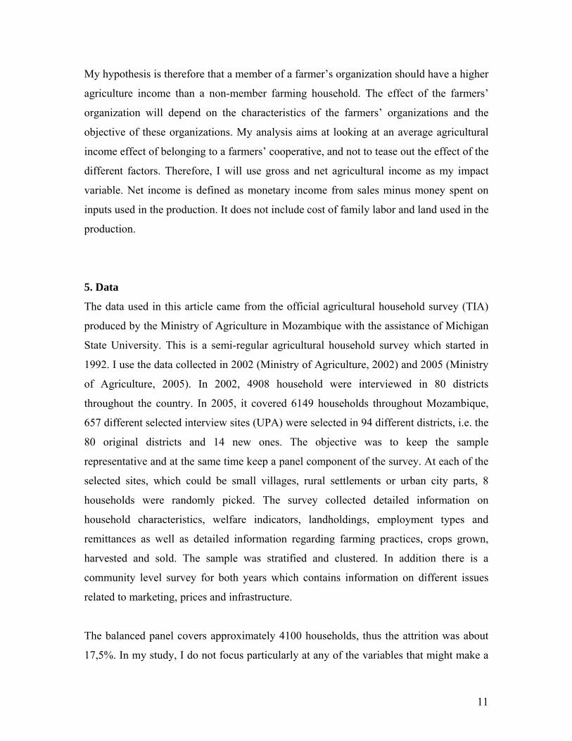
Abstract Farmers’ organizations have been suggested as a tool to improve the living conditions of farmers in poor countries, both by improving their market situation and enhancing the dissemination of information. To study this, I employ unique panel data from Mozambique. The causal effect on small-scale farmers’ income from being member in a farmers’ organization of organization membership is estimated using a difference-in-difference matching estimator. The main finding is the effect of membership among small-scale farmers on agricultural profits is positive and quite strong, while the effect on the value of plant production is not significant. This might indicate that farmers’ organizations to a larger extent focus on production or crops relevant for the market than for production for own consumption. Thus, aid to farmers’ organizations is beneficial for the farmers and farmers’ organizations are a good tool to improve small-scale farmers’ welfare.

3
Presentation of the author Maren Elise Bachke PhD-student and research fellow Department of Economics and Resource Management University of Life Sciences Aas Norway Email: [email protected] Fax: +47 64 96 57 01 Phone Number: +4764 9 65 62 P. O. Box 5003, No-1432 Aas, Norway www.umb.no I have a Master’s degree in agricultural economics from University of Life Sciences from 1999. After my masters, I work 5 years in the Ministry of Agriculture in Norway and 3 years as an APO in FAO in Mozambique. During my time in Mozambique, from 2002 to 2005, I worked in a project in the Ministry of Industry and Trade in Mozambique for two years and in my final year I was a Program Officer at the FAO Representation in Maputo, responsible for FAOs program in Swaziland.

4
1. Introduction A large share of the worlds poor live in rural areas and are small-scale farmers. It is
therefore important to increase the income of small-scale farmers to reduce poverty. One
policy that has been promoted to reach this goal is to create and support farmers’
organization or cooperatives in developing countries. The basic idea is that farmers’
organizations will strengthen the farmers’ negotiation position in relation to the buyers,
and reducing transaction costs faced by farmers. This will bring farmers closer to the
market, enable them to benefit from comparative advantages and maybe even to connect
them to the international market. Secondly, the farmers’ organizations might be a good
vehicle for donors to reach the small-scale farmers, which generally is a group that is
difficult to reach and target for the donor as they usually live in sparsely populated rural
areas with weak infrastructure.
Markets in rural Africa can be characterized as either spot markets (Fafchamps, 2004) or
missing. In addition, there is an increasing importance of out-grower schemes and
contract farming for cash crops or other high value crops such as horticultural crops. It is
in this latter market that there is a focus on possible monopsonistic exploitation of the
small scale farmer (Sivramkrishna and Jyotishi, 2008, White, 1997), and where farmers
organizations have been proposed to rectify the situation. If membership does reduce
transaction costs, this will enhance the probability of market participation. This effect on
transaction costs from being member in a farmers’ organization will be important in a
situation with missing markets and spot markets.
Cooperatives are important in the agricultural sector in the developed world. The basic
idea behind cooperatives is to strengthen farmers’ market power relative to the buyer as
so to reduce the monopsony power of the buyer. Farmers’ cooperatives in the developed
world originated from a situation somewhat similar to what we find in developing
countries today. Through organization, farmers increased their power relative to the
buyer as they consolidated as one larger seller, and in such a way they managed to get out
of the monopsony situation. Today, there are several types of farmers’ cooperatives in the
developed world, all of which respond to different market and product situations.

5
Generally, a farmer’s cooperative is an organization/firm that is owned by the farmers.
The cooperative buys the produce from the farmers according to a certain contract, and in
addition it might provide inputs and technical assistance.
There are few, if any, studies that evaluates the income effect of being member of
farmers’ organizations in developing countries in general, and not tied to a particular
organization. There is little empirical evidence for the income generating effect of
farmers’ organizations in developing countries. Most of the studies focus on evaluating
specific contracts and who can participate in the agreement (Becchetti and Costantino,
2008, Warning and Key, 2002). However, there is no agreement on whether the poor can
participate (Warning and Key, 2002) or if it generally are the richer farmers that
participate (Becchetti and Costantino, 2008). Both studies find that the participants have
higher income, but only the first shows that this is due to the participation.
The objective of this article is to evaluate the effect of farmers’ organization in
Mozambique on a household’s well-being. There have been ongoing efforts by the public
sector, NGOs and donors since the mid nineties to promote farmers organizations. In this
study, I am using agricultural household panel data (TIA) from 2002 and 2005 (Ministry
of Agriculture, 2002 and 2005) to evaluate the impact of farmers’ organizations on
agricultural income of small-scale farmers who are members. I use three different
estimators to evaluate this effect, first a cross-sectional propensity matching score
estimator, then a fixed-effects estimator and finally a difference-in-difference matching
estimator. The latter estimation method is based on Heckman et al. (1998), Heckman et
al. (1997) and Smith and Todd (2005). I find that membership has a positive significant
effect on overall agricultural profits, while the effect is not significant on other types of
income or the overall production value.
2. Literature review
There is a relatively thin literature on cooperatives in developing countries compared to
the developed world, where it is mainly a part of the agribusiness literature. This

6
literature has received renewed interest as vertical integration has become more
widespread in the agribusiness, and has also changed the causal direction between
farming and agribusiness from being led from the farm level to be led from the retail
industry (Reardon, et al., 2003). This might also have an effect on how farmers’
cooperatives form in developing countries today.
In the literature, there are expressed fears of monopsonistic exploitation of small-scale
farmers in contract schemes due to the unequal balance of power between the contractor
and the small-scale farmer. Thus, a common proposal to rectify this situation is to support
the creation of farmers organizations (Glover, 1987, Sivramkrishna and Jyotishi, 2008).
Furthermore, the effect of farmers’ organizations depends on how well they function,
how the contract negotiations between the farmers and the company for the contract are
conducted and in what context. Bingen et al. (2003) define three different type of
contracts or linkages between farmers and business based on their degree of human
capacity building, and thereby the possibilities of farmers’ organizations to emerge and
develop. Their claim is that only those types of contracts that build human capacity will
lead to long term sustainable benefit to the small-scale farmer and its community, that
also can last after the end of a project. They classify the contracts in three categories: i)
Contract/business which is profit driven, ii) Projects initiated and run by NGOs, and iii)
Process oriented human capacity development projects.
Profit driven contract/business, which by default is focused on cash crops and usually has
little or no social development dimension. This can be characterized as a monopsonic
situation. Projects initiated and run by NGOs and donors. They provide new or improved
technology to the farmers and also possible market outlets and linkages to the
agribusiness. This work is facilitated by a farmers’ organization that often is initiated as
part of the project. However, there are limited opportunities for the farmers in the
organization to decide what the focus of the work in the organization should be and to
direct the organization to focus on other relevant problems they face. The solutions and
the problem definitions relevant to the organization are provided by external mediators,

7
as well as the decisions of what to focus on in the organization. Participatory approaches
are assumed to make sure that the farmers have shared interests in the project and the
organization, an assumption which might not hold. The last type of project is the process
oriented human capacity development project. The main aim is to develop the human
capacity, and thereby the social self-help capacity of the community and farmers. These
projects often focus on literacy, marketing activities and different types of development
planning. In the long run, this might take the farmers out of the setting of monopsony due
to strengthened negotiation skills and in such a way creating more robust farmers’
organizations.
According to Sykuta and Cook (2001) the increased need for coordination in the
agricultural production chain is changing the role of cooperatives in the developed world.
They also point out that the performance of a cooperative depends upon its characteristics
and has identified the following five vaguely defined property rights; open versus closed
membership, purchasing duty, equity share, multipurpose versus unipurpose cooperatives
and membership fee. These characteristics do to a certain extent reduce some of the
moral hazard issues resulting from incentives structures for the producers. For example it
might be difficult to combined obligatory purchasing duty of the produce from the
farmers independent of quality and quantity with an open membership. The type of equity
share and membership costs of fees are also related to the degree of openness of the
farmers organizations. Finally, a multipurpose cooperative might lead to heterogeneity
among the members and therefore fight over the use of the resources rendering the
cooperative less efficient. All these factors will also influence the efficiency of farmers’
organizations in developing countries
Looking at the empirical literature on contract farming and farmers’ organization, the
main focus is on evaluating specific contract farming situations. In their study of contract
farming in Senegal, Warning and Key (2002) find that the poor are allowed to participate
in the contracting scheme and that they benefit economically. They use an IV-estimator
with a measure of honesty as the instrument for participation and estimate effects on
mean agricultural income per area. The variable honesty is measured from a discussion
8
with village leaders. Another study by Becchetti and Costantion (2008) analyze effects of
Fair Trade on Kenyan farmers that also are member of a farmers organization. Their
findings indicate that Fair Trade seems to be associated with farmers with superior
capabilities, economic and social wellbeing. However, they did not find an identifying
variable and their results therefore do not show causality. They propose to use a
difference-in-difference approach to make inference. In a study on market participation in
Mozambique, Boughton et al. (2007), find that membership in an association does not
impact market participation. However, due to the endogeneity of assets and market
participation, they cannot infer causality.
3. Mozambican agricultural and farmers’ organization
Mozambique has experienced steady and high growth rates since the end of the civil war
in 1992. However it remains a very poor country with a GNI per capita of 340 USD
(World Bank, 2007). According to Arndt et al. (2006) poverty incidence in the country
fell from around 69% to 54% between 1996-7 and 2002-2003. Annual agricultural
growth of 6% contributed significantly to the overall growth (Tarp, et al., 2002). This
growth was essential for reducing the poverty headcount among the poorest since it is the
sector that employs the largest share of people in Mozambique. In 2003, more than 70%
defined agriculture as their main economic activity and it sustained more than 80% of the
work (World Bank, 2007). Despite the large share of employment, it only makes up
21,5% of the GDP. The country also has large regional differences with a strong
concentration of growth in the Maputo province.
The agricultural sector in Mozambique is made up almost entirely by small-scale and
subsistence farmers, around 80% of all farmers, and is characterized by a high marketing
wedge which excludes many subsistence farmers from the market. Market participation is
clearly dependent upon the risk and the technology facing the farmer, and market
segmentation is high (Heltberg and Tarp, 2002). In Mozambique, it is not possible to own
land privately, only to lease it for 50 years with a guaranteed second period of another 50
years. Small-scale farmers’ access to land is governed through a mix of customary laws,

9
inheritance, buying or borrowing the land. Mozambican agricultural policy focuses on
increasing yields, through better technologies, and improving market access.
About 7,3% of the farmers belonged to a farmers’ organization in 2005 while only 4%
where members in 2002. Dorsey and Muchanga’s report from 1999 indicates that focus
on farmers’ organizations in Mozambique started as early as in the mid 1990s, and one
would expect to see effects of these efforts after 10 years of different interventions. These
efforts fall into the two latter categories of Bingen et al.’s three categories’ for market
linkages or working with farmers organizations for increasing market participation.
Furthermore, in Mozambique and in the cash crop sector such as tobacco and cotton,
there is a long tradition for contract farming that fits into the first category of Bingens’
three categories. It is difficult to assess all farmers’ organizations in Mozambique
generally as there are many different types. However, looking at the characterizations of
cooperatives from Cook and Illipoulos (2000), one would expect to see open farmers’
cooperatives with relatively low entry barriers as the operation costs are usually covered
by a NGO or donor. If there is no costs to become a member, the members do not
automatically have an equity share, in other words, they do not own the organization. The
capital in the organization is provided by and owned by the NGO or donor, if no other
status or regulations are provided for to redistribute the ownership to the members at a
certain point. Thus, it might be difficult to say that the farmers’ organizations in general
in Mozambique are member owned. Based on the information provided, it is difficult to
say anything in general on the issues of delivery duty, that is to what degree the
organizations have to buy the produce and the farmer has to sell the produce to the
organization. Finally, there are both unipurpose and multipurpose organizations, but
many tend to focus on one product or type of product only. Due to these issues, Boughton
et al. (2007) define farmers organizations as public goods in Mozambique. The public
good characteristics such as free-riding and non-excludability might affect the efficiency
and effectiveness of these organizations.

10
4. Analytic framework
The framework is based on the general factors that affect the profit for small-scale
farmers where a farmer with a vector of characteristics z and membership status
{ }0,1m∈ obtains profit
(1) ( ) ( ) ( ), ; , ' mp m Q A X z m X r m cπ = − −
Here, production Q depends on the input of land A and other inputs X, as well as his
characteristics and membership status. The latter capture the effects of improved
production technologies and the effect of farmer quality. The product price p and the
input prices r also depend on membership status to capture the different market situation
members enjoy. The cost Cm is the cost of being a member where the cost of being a
member is C1=C (1 indicates being a member) and the cost of not being a member is
C0=0 (0 indicating not being a member).
I hypothesize that membership (m) in a cooperative might influence the farmers profit
through three different channels. Firstly, by securing the farmer a better price for her
produce than the farmer otherwise would get, i.e. p(1)>p(0). This is due to an improved
negotiation position for farmers’ organizations relative to single farmers, resulting from a
larger quantity sold and lower transaction costs for the buyer. Second, membership can
provide lower prices of the inputs (r(1)<r(0)) as the cooperative buys relatively larger
quantities compared to the individual small-scale farmers. Third, the cooperative might
also provide technical assistance and technology2, so that the production function satisfies
Q(A,X;z,0)<Q(A,X;z,1) for all A, X, z. Thus, one would also expect to see higher yield
among farmers that are members of farmers’ organizations. In the equation, I have
included a variable that represent the costs of being member in a farmers’ organization cm
and at the same time set this cost to be equal to 0 as there usually are no costs related to
be a member of the organization in Mozambique.
2 Examples of technologies are inputs such as fertilizers and pesticides or extension to promote new technology.
11
My hypothesis is therefore that a member of a farmer’s organization should have a higher
agriculture income than a non-member farming household. The effect of the farmers’
organization will depend on the characteristics of the farmers’ organizations and the
objective of these organizations. My analysis aims at looking at an average agricultural
income effect of belonging to a farmers’ cooperative, and not to tease out the effect of the
different factors. Therefore, I will use gross and net agricultural income as my impact
variable. Net income is defined as monetary income from sales minus money spent on
inputs used in the production. It does not include cost of family labor and land used in the
production.
5. Data
The data used in this article came from the official agricultural household survey (TIA)
produced by the Ministry of Agriculture in Mozambique with the assistance of Michigan
State University. This is a semi-regular agricultural household survey which started in
1992. I use the data collected in 2002 (Ministry of Agriculture, 2002) and 2005 (Ministry
of Agriculture, 2005). In 2002, 4908 household were interviewed in 80 districts
throughout the country. In 2005, it covered 6149 households throughout Mozambique,
657 different selected interview sites (UPA) were selected in 94 different districts, i.e. the
80 original districts and 14 new ones. The objective was to keep the sample
representative and at the same time keep a panel component of the survey. At each of the
selected sites, which could be small villages, rural settlements or urban city parts, 8
households were randomly picked. The survey collected detailed information on
household characteristics, welfare indicators, landholdings, employment types and
remittances as well as detailed information regarding farming practices, crops grown,
harvested and sold. The sample was stratified and clustered. In addition there is a
community level survey for both years which contains information on different issues
related to marketing, prices and infrastructure.
The balanced panel covers approximately 4100 households, thus the attrition was about
17,5%. In my study, I do not focus particularly at any of the variables that might make a

12
household move or similar actions which is particularly vulnerable to attrition. Among
the members in farmers’ organization, 11% of the members were lost due to attrition.
Thus, attrition is not is higher in my main variable than in the overall sample, and as such
reducing the problem of attrition in my case.
Table 1 describes the flows of membership in farmers’ organization between 2002 and
2005 in Mozambique. The most surprising fact is that 57% of the members in 2002 left
the farmers’ organizations, and only 32% stayed as members3. Furthermore, the
overwhelming majority of the surveyed households were not members in either year.
This might indicate that it is not as beneficial to be member as proclaimed.
Table 1 Membership in 2002 and 2005
At the same time, one can clearly see from the Table
on descriptive statistics in Appendix 5, that
members generally are better off than non-members.
All the welfare indicators are higher for members
and the difference is significant. Furthermore, it
seems like they have higher education and use better agricultural technologies.
3 These numbers adds up to 89% and the missing 11% is the attrition.
Member 2005
Yes No
Member
2002
Yes 47 105
No 220 3115

13
Table 2 Comparison of mean values between members and nonmembers in farmers organizations Average Nonmembers Members t-value Head of Household Characterisicts
Age of head of household (years) 43,60 43,50 44,10 0,97
Gender of the head of the household 74,70 % 73,50 % 76,80 % 1,69 Years of schooling (School) 2,77 2,67 3,45 4,96
Self-employment among head of household (dummy variable) 38,80 % 37,70 % 44,60 % 3,26 Salary work among head of household (dummy variable) 22,10 % 22,00 % 23,90 % 1,58
Household Characteristics Average landholdings per household (ha/hh) 1,97 1,93 2,55 4,82 Number of persons in the household (number) 5,67 5,61 6,68 7,87 Welfare characteristics Radio 51,61 % 50,70 % 63,60 % 5,78 Oil lamp 48,99 % 48,48 % 57,17 % 3,95 Table 33,64 % 32,80 % 47,10 % 6,84 Latrine 41,10 % 40,20 % 54,96 % 6,78
Agricultural practices Irrigation (dummy variable) 9,37 % 8,67 % 20,51 % 9,21
Fertilizers (dummy variable) 4,16 % 3,50 % 14,70 % 12,79
Animal traction (dummy variable) 12,33 % 11,99 % 17,80 % 4,21 Pesticides (dummy variable) 6,00 % 5,50 % 13,70 % 6,87
Manure (dummy variable) 5,10 % 4,80 % 9,55 % 4,79 The sample used is a pooled sample of the 2002 and 2005 data. The t-test is testing the difference of income groups between the members and non-members in farmers organizations.
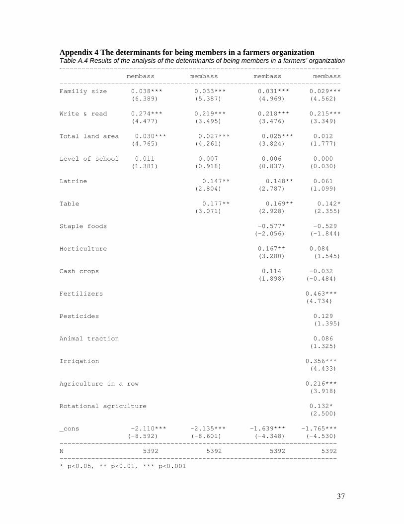
In addition to these simple t-tests, I used a probit analysis to identify the determinants of
being a member where membership was the binary dependent variable. The equation
used for the analysis was:
(2) )0()1( >+== εβXprobyprob )1,0(~ Nε
The results from the analysis of the determinants of membership in a farmers’
organization in Mozambique is presented in Appendix 5, Tables A.4 and A.5. This
analysis shows that the family size, the ability to read and write, farm size, the use of
fertilizer and irrigation, to grow crop in a row and where the farmer lives determines the
probability of being member. However, other determinants such as the farmers’ wealth

14
(table and latrine), self-employment and the type of crop grown might also influence the
propensity to be a member. From the descriptive part we can say that members of
farmers’ organizations know better to read and write than other farmers, have larger
farms, access to better agricultural technologies and have a higher tendency to grow cash
crops and horticulture than other farmers. Welfare indicators such as radios, latrines,
tables indicate that they are better off than other farmers. Thus, the donors do not reach
the poorest of the poor when working with farmers organizations.
Income
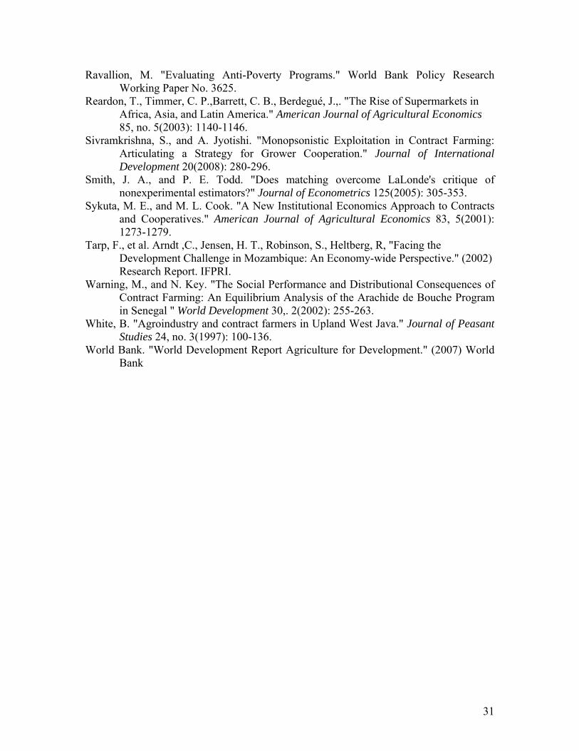
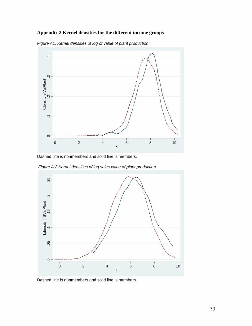
The different income variables are shown in the table below. There are four different
categories of income; i) valuation of plant production, ii) sales value of plant production,
iii) income from animal production and iv) overall agricultural profit. The value of plant
production is an estimate, among the people in the survey, of the overall value of
production of staples and cash crops, the sales value of plant production is the sales value
of all types of plant crops and includes both sales done and expected sales in the survey
year and income from animal production is the realized income from animal production.
The last category is the net agricultural profit which includes the sales value from plant
production and income from animal production minus costs of production. The costs
included are seed costs and other input costs4, however, family labour and value of own
land in production is not included. All values are measured in 1000 meticais5.
4 Currently, the cost of hired labor is not included. 5 In 2004, 1 US$ is about 24000 meticais.
15
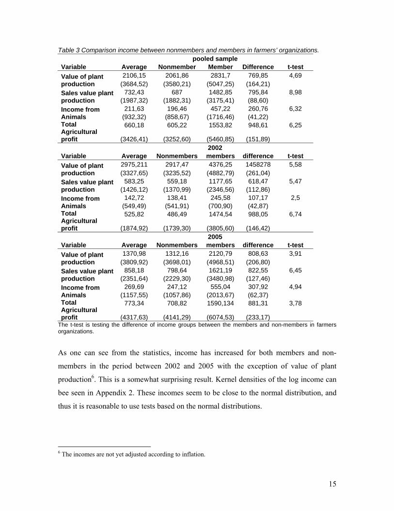
Table 3 Comparison income between nonmembers and members in farmers’ organizations. pooled sample Variable Average Nonmember Member Difference t-test Value of plant production
2106,15 2061,86 2831,7 769,85 4,69 (3684,52) (3580,21) (5047,25) (164,21)
Sales value plant production
732,43 687 1482,85 795,84 8,98 (1987,32) (1882,31) (3175,41) (88,60)
Income from Animals
211,63 196,46 457,22 260,76 6,32 (932,32) (858,67) (1716,46) (41,22)
Total Agricultural profit
660,18 605,22 1553,82 948,61 6,25
(3426,41) (3252,60) (5460,85) (151,89) 2002 Variable Average Nonmembers members difference t-test Value of plant production
2975,211 2917,47 4376,25 1458278 5,58 (3327,65) (3235,52) (4882,79) (261,04)
Sales value plant production
583,25 559,18 1177,65 618,47 5,47 (1426,12) (1370,99) (2346,56) (112,86)
Income from Animals
142,72 138,41 245,58 107,17 2,5 (549,49) (541,91) (700,90) (42,87)
Total Agricultural profit
525,82 486,49 1474,54 988,05 6,74
(1874,92) (1739,30) (3805,60) (146,42) 2005 Variable Average Nonmembers members difference t-test Value of plant production
1370,98 1312,16 2120,79 808,63 3,91 (3809,92) (3698,01) (4968,51) (206,80)
Sales value plant production
858,18 798,64 1621,19 822,55 6,45 (2351,64) (2229,30) (3480,98) (127,46)
Income from Animals
269,69 247,12 555,04 307,92 4,94 (1157,55) (1057,86) (2013,67) (62,37)
Total Agricultural profit
773,34 708,82 1590,134 881,31 3,78
(4317,63) (4141,29) (6074,53) (233,17) The t-test is testing the difference of income groups between the members and non-members in farmers organizations.
As one can see from the statistics, income has increased for both members and non-
members in the period between 2002 and 2005 with the exception of value of plant
production6. This is a somewhat surprising result. Kernel densities of the log income can
bee seen in Appendix 2. These incomes seem to be close to the normal distribution, and
thus it is reasonable to use tests based on the normal distributions.
6 The incomes are not yet adjusted according to inflation.

16
5 Impact assessment and methodology
Impact assessment methods aim at identifying and isolating the impact of projects on the
participants (Ravallion, 2005). The basic form is to asses the effect on an indicator of the
project against the counterfactual which normally is no project. The impact is the change
in the indicator, Yi1, from the participation in the project, also often called the treated.
This should then be measured against the level of the indicator, Yi0, if there is no project.
A main challenge is related to the missing data problem, it is logically impossible to have
an observation of the same person or household with and without the project.
It is this counterfactual situation one would like to approximate with a control group.
There are two main different methods for obtaining this control group, either randomized
experiments or non-experimental methods. In the non-experimental methodology, the
control group is obtained based on observable characteristics’ of the participants. A
central problem related to the control group from a non-experimental methodology is the
selection bias, which means that what is measured is not only the impact of the project, or
membership in this case, but difference in the unobservable characteristics between those
participating in the project and the control group. The randomized experiment generates a
control group that has the same distribution of observable and unobservable
characteristics as the participant group. In order to use a randomization methodology
there is a need to set this experimental design up before the project starts, define who is
given access to the program or and who is not given access. This is not the case in my
situation. I am using a non-experimental estimator to find the income effect of
membership in a farmer’s organization in Mozambique.
The estimation method I use is based on Heckman et al. (1998), Heckman et al. (1997)
and Smith and Todd (2005)’s two step estimator, where the first step is to construct a
control group by matching members of farmers’ organizations to similar farmers that are
not member of any farmers’ organization. The second step is to look at the difference in
income between the treated, the members, in relation to this control group, which is
constructed by the matching estimator.

17
Formally, let Yit1 be the household’s income in period t if it is a member of an
agricultural association and let Yit0 be the income of a household that is not member of a
farmers’ organization. The impact of being member of a farmers’ organization is then the
impact of membership is described by equation (3) where Y is the agricultural income of
person i at time t, and the up script 1 signifies that the individual is a member of a farmers
organization and 0 indicates the counterfactual, that is not being a member.
(3) 01ititit YYY −=Δ
My interest is to find the average effect of being a member of a farmers’ organization on
the members, that is the effect of being member on the agricultural income for those that
are members in a farmers’ organization. The calculations are as follows;
(4) [ ] [ ] [ ] [ ]1,1,1,1, 0101 =−===−==Δ≡ MXYEMXYEMXYYEMXYEATT ititititit
Where the X are the control factors and M=1 indicates membership in a farmers
organization. Due to the missing data problem, equation (4) cannot be estimated as one
cannot measure a person with and without the membership in any time period.
Therefore, I construct a comparison group on observables characteristics X, using a
propensity score estimator. This estimator builds on the following assumptions;
(5) [ ] [ ]0,1, 00 === MXYEMXYE itit for SX ∈
Where S is the area of common support given by )0()1( =∩== MXSuppMXSuppS .
This says that the outcome for the control group is the same as it would have been if they
where members in the area of common support. The main requirement of the assumption
is that there are no factors associated with membership status that are not included in X
that also affect income. These assumptions are necessary to compute equation (4) as it
makes it possible to approximate the latter term in the difference. The second assumption
is;
18
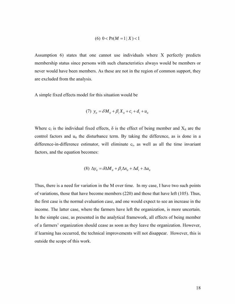
(6) 0 Pr( 1| ) 1M X< = <
Assumption 6) states that one cannot use individuals where X perfectly predicts
membership status since persons with such characteristics always would be members or
never would have been members. As these are not in the region of common support, they
are excluded from the analysis.
A simple fixed effects model for this situation would be
(7) it it t it i t ity M X c d uδ β= + + + +
Where ci is the individual fixed effects, δ is the effect of being member and Xit are the
control factors and uit the disturbance term. By taking the difference, as is done in a
difference-in-difference estimator, will eliminate ci, as well as all the time invariant
factors, and the equation becomes:
(8) it it t it t ity M x d uδ βΔ = Δ + Δ + Δ + Δ
Thus, there is a need for variation in the M over time. In my case, I have two such points
of variations, those that have become members (220) and those that have left (105). Thus,
the first case is the normal evaluation case, and one would expect to see an increase in the
income. The latter case, where the farmers have left the organization, is more uncertain.
In the simple case, as presented in the analytical framework, all effects of being member
of a farmers’ organization should cease as soon as they leave the organization. However,
if learning has occurred, the technical improvements will not disappear. However, this is
outside the scope of this work.

19
Using both these types of estimator, one gets a difference-in-difference matching
estimator. For this estimator to be valid, assumption (4) can be relaxed to7:
(9) [ ] [ ]0,1, 01
02
11
12 =−==− MPYYEMPYYE
Where t=2 is after membership decision and t=1 is before membership. An additional
requirement here is that the requirement in equation (5) regarding the area of common
support must hold in both periods. This is affected by attrition which unfortunately also is
relevant in my case. However, it should be noted that the number reported in table 1 does
not include the loss of memberships due to attrition8. The difference-in-difference
matching estimator is:
(10) ( ) ( )∑ ∑∩ ∩∈ ∈ ⎪⎭
⎪⎬⎫
⎪⎩
⎪⎨⎧
−−−=mSt mStIi
tjtjIj
titiDDM YYjiwYYn
1 0
0001
1
),(1α
Where the w(i,j) represent the weighing regime in my matching estimator. I plan to use
both the kernel matching estimator (Heckman, et al., 1998) and the nearest neighbor
estimator. It compares on members to a group of nonmembers using a kernel-weighted
average from this group. The estimator is:
(11) ∑
∑
∈
∈
−
−
=
0
0
)(
)(),(
0
Ikn
ik
Ijn
ijj
appG
app
GYjiw
Where an is the band width of the kernel and k represent the number in the kernel group.
According to Smith and Todd (2005), there are three data requirement for making the
non-experimental matching methods to perform well, particularly compared to
experimental data, and these are; 1) the data source should be the same for both the
7 Slightly changed from Smith and Todd (2005) 8 See the data section for the discussion of the attrition

20
members and the non-members making the measurement error the same for both groups,
2) members and non-members belongs to the same relevant market and 3) the data
contains a rich set of variables that can explain both membership in the organization and
the outcome (Smith and Todd, 2005). My data clearly satisfies the first, all the data is
from the same survey. The second criterion is met by including the geographical variable
province in the estimation of the propensity score. Thus, the control group is in this way
restricted to be in the same market. The third criterion is also satisfied as my data
contains a lot of information that is very relevant to the outcome, the agricultural income,
and also information relevant to becoming a member in a farmers’ organization as this
usually is related to agricultural factors such as actually farming, type of farming, land
ownership and agricultural education. It also depends on literacy, wealth, and placement
in the community, information that also is contained in the data.
There is generally not a need to have exclusion restriction when you use a matching
estimator as the matching estimator constructs a comparison group (Blundell and Costas
Dias, 2000). However, it is possible to partition the set of variables X that goes into the
estimation into two sets, and not necessarily mutually exclusive sets, but with some
exclusion restrictions (Z,W) (Heckman, et al., 1998). Where Z is the variables that
explain the membership decision and W are controls for the outcome, the agricultural
income in my case. I did this as certain variables such as network, remittances and the
feeling of increased well-being is more important to explain membership than income,
but that the agricultural factors are as important in both. Thus, I used more variables in
the propensity score (Z) than as controls in the income regressions (W), see tables x and x
for further details.
The main criticism against this method concerns whether the data material the analyst has
access to is rich enough to do the matching, i.e. that the unobservables have a significant
effect on the decision to become member or that the unobservables are strongly related to
the observables (Heckman, et al., 1998). Panel data can to a certain degree overcome this
in two ways; first, it makes it possible to choose a difference-in-difference propensity
score matching estimator. Such an estimator takes care of the problem of time-invariant

21
differences between members and non-members. Additionally, using a difference-in-
differences estimator enables control for some of the variation between good and bad
years as some where members in 2002 and some in 2005 (Smith and Todd, 2005).
7. Estimations and results
There are three sets of results, first, the cross-sectional propensity score matching
estimator, second, the results of estimations of the fixed effects model, and finally, the
results of the complete difference-in-difference matching estimator.
7.1 Cross-sectional analysis
An important part in propensity score matching is to have a good model which says why
people are treated, in my case why they participate in farmers’ organization? What are
the particular attributes that makes a farmer join a farmers’ organization? There is little
theory to guide my decision, however, I have focused on factors that are somewhat prior
to the decision to join a farmers’ organization. In Appendix 3, all the different variables I
have are presented. I have categorized these variables into four different groups of
descriptive variables, these are: i) characteristics of the head of the household, ii)
characteristics of the household, iii) diverse information and relationship inside the
village, iv) welfare indicators and v) agricultural characteristics of the household. The
variables I have defined as predetermined for the membership in farmers’ organizations
are the characteristics of the head of the household and the household as well as whether
they are born in the village, either the man or the wife. This variable tells you how well
the family is connected in the village and therefore would probably be able to say
something about the information that reaches them. Furthermore, I have included contact
with extension officers as these can provide information about farmers’ organizations as
can the ownership of a radio. I have generally not included the agricultural or other
welfare indicators as these can as much be a result of a membership in a farmers’
organization.

22
The results of the propensity score matching is presented in table 4. It is a probit
estimation9 as presented in equation (2). I have over-parameterize the regression in order
to establish good propensity score. In addition, it is necessary that the propensity score is
balanced in the two groups, members and non-members. This is called the balancing
property and it is secured with a t-test within different groups in the estimations (Gilligan
and Hoddinott, 2007, Morgan and Winship, 2007).
Table 4 Propensity score in the 2002 and 2005 sample. 2002 sample 2005 sample
Age of HHH 0,00245 0,00232 (0,95) (1,15)
Gender of HHH -0,155* -0,101 (-1,66) (-1,39)
Eduction of HHH 0,0184** 0,0127
(1,97) (1,37)
HHH has salary work 0,00357 -0,0547
-0,03 (-0,82)
HHH born in village -0,00752 (-0,10)
Spouse of HHH born in village -0,0301 (-0,38)
HHH knows to read/write 0,218*** (3,04)
Network 0,345*** (7,48)
Agriculture is primary activity -0,0843 -0,0591 (-0,92) (-0,92)
Number of HH members 0,0441*** 0,0234***
(3,25) (2,85)
Radio 0,149* 0,118* (1,89) (1,93)
Information from extension 0,697*** 0,219** (8,46) (2,3)
Total land area -0,0164 0,00967* (-0,57) (1,7)
Constant -2,081*** -2,006*** (-9,82) (-15,10)
N 4223 4924 t statistics in parentheses p<.1, ** p<.05, *** p<.01 The binary variable is membership
9 The Stata algoritm is developed by Becker and Ichino (2002).

23
The factors that are significant in both years are information from extension agent,
owning a radio, number of household members, and education (education in 2002 and
write and read in 2005). In addition, total land area and network is signification in the
2005 sample while gender of head of household is significant in the 2002 sample. The
model predicts 3,9% among the nonmembers and 7,0% among the members while the
overall membership in 2002 is 4,0%.
Based on these propensity scores, I have estimated the average impact on the treated, that
is membership, using two different matching estimators, the nearest neighbor estimator
and the kernel estimator (presented in equation (10)). The results are presented in Tables
5 and 6.
Table 5 Average impact of membership among the members using the nearest neighbor matching estimator Income variable
2002 2005 Treat/ control
ATT Treat/ control
ATT
Value of plant production
170 161
0,336*** (0,117)
369 141
0,039 (0,146)
Sales value of plant production
170 96
0,302* (0,174)
369 181
0,388** (0,158)
Income for animal production
170 69
0,370 (0,334)
369 113
-0,131 (0,186)
Total agricultural profit
170 96
0,757*** (0,200)
369 196
0,318** (0,153)
The number of treated and the number of controls are different in each estimation *** signifies significant at 1%, ** significant at 5%, *significant at 10% ATT is the average treatment effect on the treated. Treatment here is membership in a farmers’ organization.
Using the nearest neighbor algorithm, I find a significant effect of membership on log
income related to overall agricultural profit and sales value of plant production while
membership only has an effect on value of production in 2002. In all cases except for
animal income in 2005, the coefficient for membership is positive, and hence indicates
that membership leads to a higher income for the members. Furthermore, there seems to
be a significant effect on income of being member as the increase in total agricultural
profits is between 75% to 30% in all of these estimations.
24
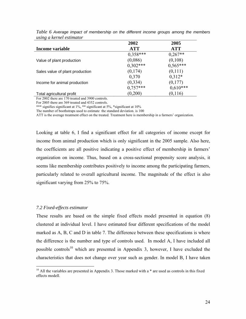
Table 6 Average impact of membership on the different income groups among the members using a kernel estimator Income variable
2002 2005 ATT ATT
Value of plant production 0,358***
(0,086) 0,267** (0,108)
Sales value of plant production 0,302***
(0,174) 0,565***
(0,111)
Income for animal production 0,370
(0,334) 0,312* (0,177)
Total agricultural profit 0,757***
(0,200) 0,610***
(0,116) For 2002 there are 170 treated and 3900 controls. For 2005 there are 369 treated and 4352 controls. *** signifies significant at 1%, ** significant at 5%, *significant at 10% The number of boothstraps used to estimate the standard deviation. is 100 ATT is the average treatment effect on the treated. Treatment here is membership in a farmers’ organization.
Looking at table 6, I find a significant effect for all categories of income except for
income from animal production which is only significant in the 2005 sample. Also here,
the coefficients are all positive indicating a positive effect of membership in farmers’
organization on income. Thus, based on a cross-sectional propensity score analysis, it
seems like membership contributes positively to income among the participating farmers,
particularly related to overall agricultural income. The magnitude of the effect is also
significant varying from 25% to 75%.
7.2 Fixed-effects estimator
These results are based on the simple fixed effects model presented in equation (8)
clustered at individual level. I have estimated four different specifications of the model
marked as A, B, C and D in table 7. The difference between these specifications is where
the difference is the number and type of controls used. In model A, I have included all
possible controls10 which are presented in Appendix 3, however, I have excluded the
characteristics that does not change over year such as gender. In model B, I have taken
10 All the variables are presented in Appendix 3. Those marked with a * are used as controls in this fixed effects modell.

25
out the agricultural controls, in model C I have taken out the welfare indicators and in
model D I have taken out both the agricultural and welfare controls.
Table 7 Impact on the different income groups of membership from a fixed-effect estimator
Model
Value plant
production
Sales value plant prod.
Income Animal prod.
Agricultural profits
specifications agri cont.
welfare cont.
HHH cont.
D 0.167 0.303** 0.445* 0.489*** no no yes (1.28) (2.14) (1.89) (3.50)
C 0.0922 0.203 0.517** 0.380*** yes no yes (0.73) (1.52) (2.07) (2.89)
B 0.141 0.287** 0.423* 0.380*** no yes yes (1.11) (2.14) (1.74) (2.89)
A 0.0801 0.198 0.504** 0.352*** yes yes yes (0.65) (1.53) (1.98) (2.72)
t statistics in parentheses * p<.1, ** p<.05, *** p<.0
ATT is the average treatment effect on the treated. Treatment here is membership in a farmers’ organization.
From table 7, one can see that membership does not have any effect on the overall value
of plant production while it is significant, thought at difference levels of significance for
both income from animal production and agricultural profits. For sales value of plant
production, it is only significant in model B and model D, indicating that the variables
used in agricultural controls are very import for the results. Additionally, the magnitude
of the coefficient for all except income from animal production is reduced as more and
more controls are included. This indicates that the controls are significant for estimating
the results. Finally, the magnitude of the significant coefficients is between 28% and 50%
which indicate that membership in a farmers’ organization raises income with 28 to 50
percent.
7.3 The difference-in-difference matching estimator
The difference-in-difference matching estimator is estimated for 3 different cases,
becoming a member in a farmers’ organization for farmers who joined between 2002 and
2005, staying as a member in a farmers’ organization between 2002 and 2005 and finally
leaving a farmers’ organization between 2002 and 2005. Table 8 the different propensity
26
scores for whether people become, stay or leave a farmers’ organization based on their
2002 characteristics.
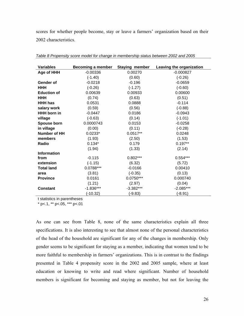
Table 8 Propensity score model for change in membership status between 2002 and 2005
Variables Becoming a member Staying member Leaving the organization Age of HHH -0.00336 0.00270 -0.000827 (-1.40) (0.60) (-0.26) Gender of -0.0218 -0.196 -0.0659 HHH (-0.26) (-1.27) (-0.60) Eduction of 0.00639 0.00933 0.00600 HHH (0.74) (0.63) (0.51) HHH has 0.0531 0.0888 -0.114 salary work (0.59) (0.56) (-0.88) HHH born in -0.0447 0.0186 -0.0943 village (-0.63) (0.14) (-1.01) Spouse born 0.0000743 0.0153 -0.0258 in village (0.00) (0.11) (-0.28) Number of HH 0.0233* 0.0517** 0.0248 members (1.93) (2.50) (1.53) Radio 0.134* 0.179 0.197** (1.94) (1.33) (2.14) Information from -0.115 0.802*** 0.554*** extension (-1.15) (6.32) (5.72) Total land 0.0788*** -0.0166 0.00410 area (3.81) (-0.35) (0.13) Province 0.0161 0.0750*** 0.000740 (1.21) (2.97) (0.04) Constant -1.836*** -3.382*** -2.085*** (-10.32) (-9.83) (-8.91) t statistics in parentheses * p<.1, ** p<.05, *** p<.01
As one can see from Table 8, none of the same characteristics explain all three
specifications. It is also interesting to see that almost none of the personal characteristics
of the head of the household are significant for any of the changes in membership. Only
gender seems to be significant for staying as a member, indicating that women tend to be
more faithful to membership in farmers’ organizations. This is in contrast to the findings
presented in Table 4 propensity score in the 2002 and 2005 sample, where at least
education or knowing to write and read where significant. Number of household
members is significant for becoming and staying as member, but not for leaving the

27
organizations. Radio is important to become and to leave the organizations, but not for
staying as a member. Land seems important for becoming a member, but not for later
changes in status. All these characteristics confirm the earlier results. Information from
extension services is important both for staying and for leaving the organizations, but not
becoming a member. This is contrary to what I found earlier. Generally, it is surprising
that the personal characteristics of the farmers’ are of relatively little importance for
membership. I would also like to point out that province the farmer is in seems to be
crucial for the farmers to stay members, which might indicate that this has to do with
options to stay as a member.
Table 9 Impact on income from changes in membership estimated by the nearest neighbor estimator
Income variables
Becoming a member Staying a member Leaving the organization
treat./cont. ATT treat./cont. ATT treat./cont. ATT Value plant production 218 0,343 47 -0,720** 104 -0,408 (lnValPlant) 64 (0,226) 16 (0,322) 40 (0,286) Sales value plant prod. 218 0,247 47 0,323 104 -0,118
(lnSValPlant) 70 (0,246) 17 (0,465) 36 (0,308) Income
Animal prod. 218 1,360*** 47 -0,326 104 -0,370 (lnIncAni) 28 (,427) 2 (0,464) 14 (0,364)
Agricultural profits 218 0,520** 47 0,200 104 -0,452
(lnprofitTag) 62 (0,250) 14 (0,558) 29 (0,380) p<.1, ** p<.05, *** p<.01 ATT is the average treatment effect on the treated. Treatment here is membership in a farmers’ organization.
From Table 9, we can see that becoming a member in a farmers’ organization leads to a
positive shift in income from animal production and overall agricultural profits. It does
not seem like leaving the organization affects income at all, however, we can see that all
the coefficients are negative. Staying as a member seems surprisingly to lead a significant
negative shift in value of plant production. The magnitude of the positive effect on
agricultural profits is still in the area of 50%, matching the earlier results. However, the
magnitude of the income from animal production is surprisingly 136% and clearly the
highest impact found so far.

28
Table 10 Impact on income from changes in membership estimated by the kernel estimator Income variables Becoming a member Staying member Leaving the organization ATT ATT ATT
Value plant production 0,202 -0,342 -0,217 (lnValPlant) (0,16) (0,243) (0,247) Sales value plant prod. 0,281 0,365 -0,444
(lnSValPlant) (0,224) (0,276) (0,239) Income Animal
prod. 0,293 0,025 -0,534 (lnIncAni) (0,319) (0,744) (0,362)
Agricultural profits 0,506*** 0,306 -0,534**
(lnprofitTag) (0,185) (0,354) (0,534) p<.1, ** p<.05, *** p<.01 ATT is the average treatment effect on the treated. Treatment here is membership in a farmers’ organization.
Using the kernel estimator, the only significant results are for agricultural profits, where
becoming a member gives a positive shift in income while leaving the organization gives
a negative shift in income. The magnitude of this effect is still around 50%, which is
substantial and matches the earlier results, while the magnitude of leaving the
organization is around the same level. Thus, it seems like membership shifts the income
path upwards, but once a member, the income does not keep growing faster than other
farmers. If you leave, there will be a negative shift in income taking you back to the
original path.
8. Conclusion
My estimations seem to indicate that there is a positive causal effect from membership in
a farmers’ organization to overall agricultural profits. This group of income is always
significant and positive. Furthermore, the magnitude of this effect is high and around
50% for agricultural profits. It varies from around 35% to 75% in the different estimators,
but in most cases it is stable around 50%. For the other types of income, the results are
more variable. The impact on income from animal production is significant in the fixed-

29
effect model and the difference-in-difference propensity score model, but not in the
cross-section model. However, it seems like membership might have a positive effect on
income from animal production and that it is contributing to the overall effect on
agricultural profits. Mostly, the effect of membership is around 50% for income from
animal production, except for the unusual high effect in the difference-in-difference
nearest neighbor estimator. For the sales value of plant production the results are
somewhat opposite those from animal production. The results are significant when using
the cross-sectional estimators, but not in the difference-in-difference estimator. The effect
of membership on income is stable and around 30% when the results are significant.
Finally, there are probably not large effects of membership in a farmers’ organization on
the value of plant production, however, when the results are significant, the magnitude of
the impact is around 30% increase in the value of plant production.
As we can see from the results, there seems to be a positive, significant and a rather high
income potential of membership in farmers’ organization. From my results, it seems like
farmers’ organizations put more efforts into marketable goods than production for home
consumption, as well as they might focus more on plant production than animal
production. Finally, we can say that members of farmers’ organizations are wealthier than
other farmers.
From my research, we find that farmers’ organizations do contribute significantly
towards higher income, and thereby welfare among small-scale farmers. Thus, farmers’
organizations are a good tool to enhance small-scale farmers’ welfare. Supporting
farmers’ organizations is therefore an efficient policy to reduce poverty among small-
scale farmers, and these efforts should be strengthened. However, my research does not
tell us how this increased welfare arises. Which path is the most efficient, the price path,
the technology path or a combination? What are the most important characteristics of a
farmers’ organization for it to succeed and the project that supports the organizations?
These are questions that still need to be addressed to give policy makers more detailed
policy advice on how to best support of farmers’ organizations, beyond the fact that it is
working.

30
References Arndt, C., R. C. James, and K. Simler, R. . "Has Economic Growth in Mozambique been
Pro-Poor?" Journal of African Economies 15, no. 4(2006): 571-602. Becchetti, L., and M. Costantino. "The Effects of Fair Trade on Affiliated Producers: An
Impact Analysis on Kenyan Farmers." World Development 36, no. 5(2008): 823-843.
Becker, S. O., and A. Ichino. "Estimation of Average Treatment Effects Based on Propensity Scores." The Stata Journal 2, no. 4(2002): 1-19.
Bingen, J., A. Serrano, and J. Howard. "Linking farmers to markets: different approaches to human capital development." Food Policy 28(2003): 405-419.
Blundell, R., and M. Costas Dias. "Evaluation Methods for Non-Experimental Data." Fiscal Studies 21, no. 4(2000): 427-468.
Boughton, D., Mather,D., Barrett,C.B., Benfica,R., Abdula, D. Tschirley, D., Cunguara, B. "Market Participation by Rural Households in a Low-Income Country: An Asset-Based Approach Applied to Mozambique." Faith and Economics 50(2007): 64-101.
Cook, M. L., and C. Ilipoulos. Ill-defined Property Rights in Collective Action: the case of US Agricultural Cooperatives. Institutions, Contracts and Organizations:Perspectives from New Institutional Economics. Edited by C. Ménard. Cheltenham: Edward Elgar, 2000.
Dorsey, J., and S. P. Muchanga. "Best Practices in Farmers Association Development in Mozambique." (1999) ARD-RAISE Consortium
Fafchamps, M. Market Institutions in Sub-Saharan Africa. Theory and Evidence. Cambride, Massachusetts: The MIT Press, 2004.
Gilligan, D. O., and J. Hoddinott. "Is There Persistence in the Impact of Emergency Food Aid? Evidence on Consumption, Food Security, and Assets in Rural Ethiopia." American Journal of Agricultural Economics 89, no. 2(2007): 225-242.
Glover, D. J. "Increasing the Benefits to Smallholders from Contract Farming: Problems for Farmers' Organizatins and Policy Makers." World Development 15, 4(1987): 441-448.
Heckman, J. J., H. Ichimura, and P. Todd. "Matching As An Econometric Evaluation Estimator." Review of Economic Studies 65(1998): 261-294.
Heckman, J. J., H. Ichimura, and P. Todd. "Matching As An Econometric Evaluation Estimator: Evidence from Evaluating a Job Training Programme." Review of Economic Studies 64(1997): 605-654.
Heltberg, R., and F. Tarp. "Agricultural supply response and poverty in Mozambique." Food Policy 27, no. 2(2002): 103-123.
Ministry of Agriculture (MINAG), 2002. Trabalho de Inquérito Agrícola 2002. Departemento de Estatisitica Direccao de Economia (MINAG), República de Mocambique, Maputo, Mozambique.
Ministry of Agriculture (MINAG), 2005. Trabalho de Inquérito Agrícola 2005. Departemento de Estatisitica Direccao de Economia (MINAG), República de Mocambique, Maputo, Mozambique.
Morgan, S.L., and C. Winship. Counterfactuals and Causal Inference. Methods and
Principles for Social Research. New York: Cambridge University Press, 2007.
31
Ravallion, M. "Evaluating Anti-Poverty Programs." World Bank Policy Research Working Paper No. 3625.
Reardon, T., Timmer, C. P.,Barrett, C. B., Berdegué, J.,. "The Rise of Supermarkets in Africa, Asia, and Latin America." American Journal of Agricultural Economics 85, no. 5(2003): 1140-1146.
Sivramkrishna, S., and A. Jyotishi. "Monopsonistic Exploitation in Contract Farming: Articulating a Strategy for Grower Cooperation." Journal of International Development 20(2008): 280-296.
Smith, J. A., and P. E. Todd. "Does matching overcome LaLonde's critique of nonexperimental estimators?" Journal of Econometrics 125(2005): 305-353.
Sykuta, M. E., and M. L. Cook. "A New Institutional Economics Approach to Contracts and Cooperatives." American Journal of Agricultural Economics 83, 5(2001): 1273-1279.
Tarp, F., et al. Arndt ,C., Jensen, H. T., Robinson, S., Heltberg, R, "Facing the Development Challenge in Mozambique: An Economy-wide Perspective." (2002) Research Report. IFPRI.
Warning, M., and N. Key. "The Social Performance and Distributional Consequences of Contract Farming: An Equilibrium Analysis of the Arachide de Bouche Program in Senegal " World Development 30,. 2(2002): 255-263.
White, B. "Agroindustry and contract farmers in Upland West Java." Journal of Peasant Studies 24, no. 3(1997): 100-136.
World Bank. "World Development Report Agriculture for Development." (2007) World Bank

32
Appendix 1 Definitions from the TIA 2005 Table A.1 Definition of Household type or more exactly farm type Factors Limit 1 Limit 2 Total area of cultivated land (ha) 10 50 Number of cattle 10 100 Number of small animals such as goats, sheep and pigs
50 500
Number of poultry 5000 20000 If all the factors are below limit 1, the farm is a small-scale farm. If one of the factors are equal to or above limit 1 but lower than limit 2, the farm is medium sized. If one factor is bigger or equal to limit 2, the farm is a large scale farm. Table A.2 Overview over the provinces in Mozambique Province Number Niassa 1 Cabo Delgado 2 Nam pula 3 Zambezia 4 Tete 5 Manica 6 Sofala 7 Inhambane 8 Gaza 9 Maputo 10
33
Appendix 2 Kernel densities for the different income groups Figure A1. Kernel densities of log of value of plant production
0.1
.2.3
.4kd
ensi
ty ln
Val
Pla
nt
0 2 4 6 8 10x
Dashed line is nonmembers and solid line is members. Figure A.2 Kernel densities of log sales value of plant production
0.0
5.1
.15
.2.2
5kd
ensi
ty ln
SVa
lPla
nt
0 2 4 6 8 10x
Dashed line is nonmembers and solid line is members.

34
Figure A.3 Kernel densities of log income from animal production
0.0
5.1
.15
.2.2
5kd
ensi
ty ln
IncA
ni
0 2 4 6 8 10x
Dashed line is nonmembers and solid line is members. Figure A.4 Kernel densities of log overall agricultural profit
0.0
5.1
.15
.2.2
5kd
ensi
ty ln
prof
itTag
-5 0 5 10x
Dashed line is nonmembers and solid line is members.

35
Appendix 3 The different characteristics of the farmers Table A.3 Overview over the different characteristics of the farmers. Variable group 2002 2005 Head of HH Characteristics
- sex - age - schooling - civil status - salary work - self employed - whether the HHH is
born in the village - whether the spouse is
born in the village.
- Sex - age - schooling* - civil status - salary work* - self-employed* - Knowledge of writing or reading - Agricultural education of 3
months
Household Characteristics
- The importance of agriculture in the HH
- number of family members
- rural or urban HH - the change in members
in the HH - the number of sick HH
members
- the importance of agriculture in the HH
- number of family members* - the change in members in the HH - - the number of sick HH
members
Divers Information
- Information from extension services
- membership in farmers’ organizations
- which person is a member
- price information received
- network variable base on where family members were born
- Information from extension services*
- Membership in farmers’ organizations
- which person is a member* - price information from radio - if they did receive credit - and if so from where - network variable*
Welfare Characteristics
- oil lamp - radio - latrine - table - ownership of land - -satisfaction in the last
3 years
- oil lamp* - radio* - latrine* - table * - ownership of land - satisfaction in the last 3 years* - basic staple food - reserve of food in house - survival mechanism - problem with hunger last year - meal a day during the shortage
period of food Agricultural - Total area of land - total area of land holdings*

36
Characteristics holdings - number of cattle, - number of chicken - overall number of
animals - size of family labor - use of irrigation - fertilizer - manure - pesticides - animal traction - mechanization - hired labor full and
part time - experienced serious
production loss the last year.
- number of cattle - number of chicken* - overall number of animals* - size of family labor* - use of irrigation* - fertilizer* - manure* - pesticides* - animal traction* - hired labor - experienced serious production
loss the last year* - grow the crops in a line
*Those characteristics that are marked with a * are used in the fixed effects model.
37
Appendix 4 The determinants for being members in a farmers organization Table A.4 Results of the analysis of the determinants of being members in a farmers’ organization -----------------------------------------------------------------------
membass membass membass membass ----------------------------------------------------------------------- Familiy size 0.038*** 0.033*** 0.031*** 0.029*** (6.389) (5.387) (4.969) (4.562) Write & read 0.274*** 0.219*** 0.218*** 0.215*** (4.477) (3.495) (3.476) (3.349) Total land area 0.030*** 0.027*** 0.025*** 0.012 (4.765) (4.261) (3.824) (1.777) Level of school 0.011 0.007 0.006 0.000 (1.381) (0.918) (0.837) (0.030) Latrine 0.147** 0.148** 0.061 (2.804) (2.787) (1.099) Table 0.177** 0.169** 0.142* (3.071) (2.928) (2.355) Staple foods -0.577* -0.529 (-2.056) (-1.844) Horticulture 0.167** 0.084 (3.280) (1.545) Cash crops 0.114 -0.032 (1.898) (-0.484) Fertilizers 0.463*** (4.734) Pesticides 0.129 (1.395) Animal traction 0.086 (1.325) Irrigation 0.356*** (4.433) Agriculture in a row 0.216*** (3.918) Rotational agriculture 0.132* (2.500) _cons -2.110*** -2.135*** -1.639*** -1.765*** (-8.592) (-8.601) (-4.348) (-4.530) ---------------------------------------------------------------------- N 5392 5392 5392 5392 ---------------------------------------------------------------------- * p<0.05, ** p<0.01, *** p<0.001

38
Table A.5 Results of the analysis of the determinants of being members in a farmers’ organization ------------------------------------------------------------------------- (1) (2) (3) (4) membass membass membass membass b/t b/t b/t b/t ------------------------------------------------------------------------- Family size 0.032*** 0.029*** 0.029*** 0.028*** (5.000) (4.471) (4.382) (4.212) Write & read 0.243*** 0.215*** 0.217*** 0.215** (3.834) (3.337) (3.356) (3.251) Salary work -0.008 -0.009 -0.000 0.021 (-0.133) (-0.140) (-0.005) (0.336) Self-employment 0.150** 0.146** 0.132* 0.126* (2.821) (2.722) (2.455) (2.286) Total land area 0.028*** 0.027*** 0.024*** 0.015* (4.330) (4.139) (3.678) (2.085) School (level) 0.005 0.004 0.003 -0.001 (0.697) (0.468) (0.416) (-0.157) Cabo Delgado (2) -0.347** -0.333* -0.299* -0.281* (-2.606) (-2.477) (-2.201) (-1.982) Zambezia(4) -0.459*** -0.446*** -0.406** -0.391** (-3.562) (-3.323) (-2.993) (-2.798) Tete (5) -0.095 -0.090 -0.098 -0.260* (-0.800) (-0.740) (-0.803) (-2.020) Manica (6) -0.456** -0.446** -0.439** -0.467** (-3.242) (-3.076) (-2.978) (-3.021) Sofala (7) -0.736*** -0.713*** -0.759*** -0.781*** (-4.820) (-4.502) (-4.731) (-4.717) Inhambane (8) -0.380** -0.376** -0.308* -0.363* (-2.808) (-2.739) (-2.209) (-2.417) Gaza (9) 0.312** 0.305** 0.337** 0.336* (2.729) (2.592) (2.763) (2.536) Maputo (10) 0.432*** 0.416** 0.435*** 0.345* (3.456) (3.272) (3.374) (2.537) Latrine 0.039 0.026 -0.051 (0.680) (0.447) (-0.860) Table 0.126* 0.123* 0.113 (2.061) (2.014) (1.806) Staple -0.329 -0.276

39
(-1.161) (-0.954) Horticulture 0.096 0.049 (1.709) (0.835) Cash crop 0.225*** 0.076 (3.499) (1.102) Fertilizer 0.378*** (3.625) Pesticides 0.173 (1.801) Irrigation 0.174* (2.033) Manure 0.219 (1.875) Agriculture row 0.288*** (4.967) _cons -1.856*** -1.865*** -1.635*** -1.723*** (-6.953) (-6.895) (-4.178) (-4.265) ------------------------------------------------------------------------- N 5392 5392 5392 5392 -------------------------------------------------------------------------- * p<0.05, ** p<0.01, *** p<0.001

40
Appendix 5 Detailed household characteristics Table A.6 Detailed household characteristics Household Characteristics Pooled sample 2005 sample 2002 sample Average No Yes t-value Average No Yes t-value Average No Yes t-value Age of head of household (years) 43,50 43,50 44,10 -0,97 46,12 % 45,97 % 47,67 % -2,41 42,57 42,54 43,46 -0,79
Gender of the head of the household 74,70 % 73,50 % 76,80 % -1,69 78,24 % 77,68 % 83,79 % -3,1793 74,20 % 74,20 % 74,26 % -0,02
Years of schooling (School) 2,77 2,67 3,45 -4,96 2,79 2,73 3,55 -4,45 2,63 2,60 3,24 -4,96
Self-employment among head of household (dummy variable) 38,80 % 37,70 % 44,60 % 3,26 42,38 % 42,08 % 45,26 % -1,3771 32,34 % 32,80 % 36,26 % -1,11
Salary work among head of household (dummy variable) 22,10 % 22,00 % 23,90 % -1,58 25,05 % 25,25 % 23,12 % 1,0531 15,48 % 15,47 % 15,78 % -0,11
Household Characteristics
Average landholdings per household (ha/hh) 1,97 1,93 2,55 4,82 2,52 2,39 3,76 -9,83 1,52 1,51 1,65 -1,34
Number of persons in the household (number) 5,67 5,61 6,68 -7,87 6,7 6,6 8,5 -10,99 5,1 5,06 5,9 -4,06 Welfare characteristics Radio 51,61 % 50,70 % 63,60 % -5,78 56,59 % 55,55 % 66,92 % -5,06 49,49 % 48,99 % 61,40 % -3,18 Oil lamp 48,99 % 48,48 % 57,17 % -3,95 50,58 % 49,61 % 60,19 % -4,67 50,86 % 50,41 % 60,23 % -2,5 Table 33,64 % 32,80 % 47,10 % -6,84 42,02 % 40,28 % 59,25 % -6,4238 29,99 % 29,53 % 48,90 % -3,19 Latrine 41,10 % 40,20 % 54,96 % -6,78 45,19 % 43,86 % 58,32 % -6,4224 38,43 % 32,90 % 50,87 % -3,42 Agricultural practices
Irrigation (dummy variable) 9,37 % 8,67 % 20,51 % -9,21 8,48 % 7,01 % 22,89 % -12,709 12,64 % 12,08 % 25,88 % -5,32

41
Fertilizers (dummy variable) 4,16 % 3,50 % 14,70 % -12,79 5,57 % 4,41 % 17,01 % -12,268 3,87 % 3,40 % 15,20 % -7,89
Animal traction (dummy variable) 12,33 % 11,99 % 17,80 % -4,21 19,83 % 18,68 % 31,21 % -6,9579 13,43 % 13,14 % 20,46 % -2,75
Pesticides (dummy variable) 6,00 % 5,50 % 13,70 % -6,87 6,95 % 6,16 % 14,77 % -7,4907 6,30 % 5,68 % 16,96 % -6,04
Manure (dummy variable) 5,10 % 4,80 % 9,55 % -4,79 4,47 % 3,98 % 9,35 % -5,7428 6,88 % 6,56 % 14,61 % -4,09