1181

Are dispersion corrections accurate outside equilibrium?A case study on benzeneTim Gould*1, Erin R. Johnson2 and Sherif Abdulkader Tawfik3,4

Full Research Paper Open Access

Address:1Queensland Micro- and Nanotechnology Centre, Griffith University,Nathan, Queensland 4111, Australia, 2Department of Chemistry,Dalhousie University, Halifax, Nova Scotia, B3H 4R2, Canada,3School of Mathematical and Physical Sciences, University ofTechnology Sydney, Ultimo, New South Wales 2007, Australia and4Institute for Biomedical Materials and Devices (IBMD), Faculty ofScience, University of Technology Sydney, Sydney, NSW, Australia

Email:Tim Gould* - t.gould@griffith.edu.au

* Corresponding author

Keywords:benzene; DFT; dispersion; van der Waals

Beilstein J. Org. Chem. 2018, 14, 1181–1191.doi:10.3762/bjoc.14.99

Received: 22 February 2018Accepted: 30 April 2018Published: 23 May 2018

This article is part of the Thematic Series "Dispersion interactions".

Guest Editor: P. Schreiner

© 2018 Gould et al.; licensee Beilstein-Institut.License and terms: see end of document.

AbstractModern approaches to modelling dispersion forces are becoming increasingly accurate, and can predict accurate binding distances

and energies. However, it is possible that these successes reflect a fortuitous cancellation of errors at equilibrium. Thus, in this work

we investigate whether a selection of modern dispersion methods agree with benchmark calculations across several potential-energy

curves of the benzene dimer to determine if they are capable of describing forces and energies outside equilibrium. We find the

exchange-hole dipole moment (XDM) model describes most cases with the highest overall agreement with reference data for ener-

gies and forces, with many-body dispersion (MBD) and its fractionally ionic (FI) variant performing essentially as well. Popular

approaches, such as Grimme-D and van der Waals density functional approximations (vdW-DFAs) underperform on our tests. The

meta-GGA M06-L is surprisingly good for a method without explicit dispersion corrections. Some problems with SCAN+rVV10

are uncovered and briefly discussed.

1181

IntroductionThe past decade has seen an increasing awareness of the role

played by van der Waals dispersion forces in chemistry and ma-

terials science [1-6]. It has consequently become firmly estab-

lished that including dispersion forces can be vital for under-

standing and predicting the behaviour and structure of mole-

cules, materials and surfaces [7-12].

The increased attention being paid to dispersion forces has

paralleled, and been driven by, an increased interest in how to

accurately model them. Multiple families of approaches for in-

cluding dispersion forces in quantum chemical simulations

now exist, mostly based around the principle of improving den-

sity functional theory (DFT) calculations (see, e.g., some

key and recent summaries [3,5,13,14]) through a dispersion

correction. The latest variants of these approaches have

been highly successful in predicting key properties of a

wide range of molecules and materials, such as binding

energies and molecular/material structures [4,5,15]. Methods

Beilstein J. Org. Chem. 2018, 14, 1181–1191.

1182

are increasingly converging towards accurate prediction of

these properties [16].

What is less well known, however, is how well methods predict

the properties of systems outside of internal equilibrium, i.e.,

whether they can predict energies and forces when a system has

not relaxed to its lowest energy geometry. This question is im-

portant as it is feasible that methods benefit from a cancellation

of errors at equilibrium, which may give false expectations

about their general accuracy. We therefore need to understand

the limitations of approaches in dealing with dispersion forces

generally, and not just for systems at their equilibrium geome-

tries. This is especially important for predicting how a system

(or sub-system) behaves when subject to external forces, or

when dispersion forces compete with other weak forces within

molecules or structures. It is particularly relevant as recent work

has shown that modern approaches can often provide accurate

binding distances or binding energies in layered materials [17],

but not both, suggesting limits to their accuracy.

The work by Řezáč et al. goes some way to resolving this ques-

tion, by providing benchmark values (the S66x8 set) for eight

equilibrium and non-equilibrium geometries of different molec-

ular pairs [18]. This set has been used to test various dispersion

methods [19]. However, while S66x8 certainly improves on

tests only at optimized geometries, it may still fail to expose

issues with forces or other energetic differences.

In this work we thus test the accuracy of modern dispersion

approaches in reproducing the energetics of the benzene dimer,

an important model system, in different geometries. The

coupled-cluster with singles, doubles and perturbative triples

[CCSD(T)] benchmark set of Sinnokrot et al. [20] is used, with

the aim of establishing which approximations can best repro-

duce the full potential energy curves. This simple test is not de-

signed to be comprehensive, but rather to interrogate the predic-

tive ability of different approaches. Note that the benchmark

set, while slightly inaccurate by modern standards, is predicted

to be within 0.1 kcal/mol of more recent benchmarks [21],

which is similar to methodological errors caused by using

modern pseudopotential methods [22]. We thus feel that its

range more than makes up for any limitations it may have.

Moreover, interactions between ring structures feature widely

across organic chemistry [23-25]. Recently, there has been in-

creasing interest in utilizing non-covalent π-stacking for synthe-

tic catalysis – and it is notable that most structures shown in a

recent review on the topic feature rings that interact at distances

greater than the potential minimum [26]. Benzene dimers also

feature in the S22 benchmark set [21,27] that is often used to

semi-empirically optimize dispersion corrections, and is almost

always used as a test of such methods. They are thus an excel-

lent test of the quality of dispersion models on a system where

failures may have chemical relevance.

Results and DiscussionThe origin of dispersion forcesDispersion forces are a semi-classical effect coming from quan-

tum fluctuations. Most simply, they can be viewed from the

perspective of pairs of interacting fluctuating dipoles, in which

a temporary dipole in one (sub)system induces a dipole in the

other, and consequently lowers the total energy. Since the field

from each temporary dipole falls off as the inverse cube of the

distance D between the systems, and the contributions come in

pairs, this leads to an interaction with the asymptotic form

UvdW = −C6D−6, where C6 is a coefficient that depends on the

properties of the independent systems. A similar semi-classical

analysis can also be applied to more general multipoles, such as

quadropoles, which give rise to terms proportional to D−8

(quadropole with dipole), D−10 (quadrupole–quadropole) etc.

In addition to direct coupling between pairs of multipoles, more

general forms of coupling can also lead to higher order contri-

butions, including 3rd-order effects between three multipoles,

4th-order etc., as detailed in, e.g., Dobson and Gould [2]. In

certain cases, including graphene [28-31], this can lead to

fundamental deviations from the simple model outlined above

[18,31-36]. However, the most extreme deviations from the

pairwise model do not affect the benzene dimer system.

Note, the importance of higher-order (many-body) dispersion

terms in “typical” systems has been the subject of some debate.

It is critical to differentiate between non-additive many-body

electronic interactions [34,35] and non-additive C9 or Axilrod-

Teller-Muto (ATM) dispersion interactions here. The former

cause large differences in the effective pairwise C6 and higher-

order dispersion coefficients, relative to corresponding values

for free atoms [33,37,38] (these are known as Type-B non-addi-

tivity effects in the classification scheme of Dobson [33]). This

is a particularly significant effect for metals and can alter the C6

coefficients by more than an order of magnitude in some cases

[39,40]. In contrast, the 3-body C9 contribution to the disper-

sion energy is typically smaller in magnitude than the pairwise

C10 contribution [41] and consequently is negligible for most

applications compared to 3-body electronic effects [42-44].

Mathematically, the ATM treatment is most applicable when

the energy contribution from 3rd and higher order terms

converge rapidly as a function of inverse distance and may thus

be truncated after the 2nd-order or 3rd-order contributions.

Many-body effects arise from a divergence or slow conver-

gence in the same series due to Dobson-B or -C effects, so that

Beilstein J. Org. Chem. 2018, 14, 1181–1191.

1183

the contributions must be treated as a formal power series and

rewritten as an explicit function of the polarisability tensor.

Summary of modern dispersion methodsOver the last decade, a number of new approaches have been

developed that explicitly introduce dispersion forces into elec-

tronic structure theory methods – typically density functional

theory (DFT). These approaches seek to overcome the funda-

mental lack of dispersion forces in DFT and Hartree–Fock

theory by introducing an explicit long-range correction, giving a

total energy E = EDFT + ΔEvdW for the system. Typically, EDFT

is taken from a standard density functional approximation

(DFA), such as PBE [45] or B3LYP [37], while ΔEvdW is one

of a range of dispersion correction models. Note, this is differ-

ent to seamless approaches like MP2, RPA or other quantum

chemistry methods which include dispersion forces automati-

cally.

Common van der Waals corrections can be broadly divided into

three categories, as will be detailed below. Substantial effort has

seen steady improvements in the quality of approaches in all

three categories. In this paper we focus only on recent (or older,

but still very popular) iterations within each category, to reflect

how the methods are designed to be used in practice. The three

classes of approaches considered are:

1) Purely empirical corrections based only on semi-classical

models of the nuclei, and their neighbours, without drawing

from the electronic density [15,46-50]. Of these we include

Grimme’s D2, D3 and D3-BJ functionals, as corrections on

PBE and, in the case of D3-BJ, on B3LYP. Here and hence-

forth “on X” means that the correction is taken on top of the X

(hybrid) density functional approximation, which we also

denote as X-Y (e.g., PBE-D3-BJ);

2) atomic-dipole with density methods, which correct first-prin-

ciples or empirical models of atomic dipoles (and sometimes

multipoles) using properties of the electronic density. Of these

we include XDM [51,52] (on various DFAs), TS [53] (on PBE),

TS-MBD@rsRSC (MBD for shor t , on PBE) and

FI-MBD@rsRSC (FI for short, on PBE). Both MBD [54,55]

and FI [56,57] include dispersion contributions to all orders

using the many-body dispersion method of Tkatchenko et al.

[54], but involve different treatment of polarisabilities and

screening; and

3) first principles density functionals, in which dispersion forces

depend only on the density in a totally seamless fashion [58-60]

and in which the base DFA forms part of the functional itself.

We include the functional of Dion et al. [59], vdW-DF2 [61],

optPBEvdW [62] and optB88vdW [62]. We also include

SCAN+rVV10, based on the strongly-constrained and

normalised (SCAN) meta-GGA, which has been shown to be

very successful in initial testing [63]. We refer collectively to

these as vdW-DFAs.

In addition to the van der Waals functionals, we also show ener-

gies from the generalized gradient approximations (GGAs) PBE

and B3LYP, and the meta-GGAs M06L [64] and SCAN [65]

without dispersion corrections. Although both GGAs are known

to neglect dispersion physics, the meta-GGAs M06-L and

SCAN are expected to capture some dispersion-binding contri-

butions through the large-gradient behaviour of their exchange

functionals. Note, the interplay between exchange-correlation

functionals and dispersion corrections has been the topic of

some discussion [66,67]. Finally, we note that we include only

general functionals, and avoid approaches that are designed to

address one type of system (e.g., molecules, bulks or layered

structures) only.

Calculation detailsWe performed most calculations using VASP 5.4 [68,69] where

the valence electrons are separated from the core by use of

projector-augmented wave pseudopotentials (PAW) [70]. The

energy tolerance for the electronic structure determinations was

set at 10−7 eV. Calculations used only the Γ k-point. ENCUT

was set to 400 eV in all calculations, which were carried out in

a 15 × 15 × 25 Å3 supercell. SCAN(+rVV10) required ENCUT

= 700 eV as results showed significant noise with the standard

energy cutoff, which led us to reduce the box dimensions to

12 × 12 × 20 Å3. We will discuss issues with SCAN later. Both

MBD approaches (TS-MBD and FI-MBD) used the reciprocal

space implementation [71], the latter in a custom version of

VASP 5.4.1 [57]. The vdW-DFs use the implementation of

Klimeš [72] of the Román-Pérez and Soler [73] method.

Some methods are not implemented in VASP and in these

cases, the calculations were performed using other codes. XDM

results were obtained using Gaussian09 (PBE, B3LYP, and

LC-wPBE) or Psi4 [74] (B86bPBE) and the postg application.

We include XDM results on several base functionals due to its

broad success. M06-L results were calculated with Gaussian16

using the aug-cc-pVTZ basis set due to convergence difficul-

ties with the plane-waves/pseudopotential approach.

To put these settings in context, we purposefully employed the

methods as they are intended to be used, i.e., using more-or-less

standard convergence parameters and recommended settings.

ResultsNow that we have established the background methodology, let

us summarise the shared features of Figures 1–3 to aid in

Beilstein J. Org. Chem. 2018, 14, 1181–1191.

1184

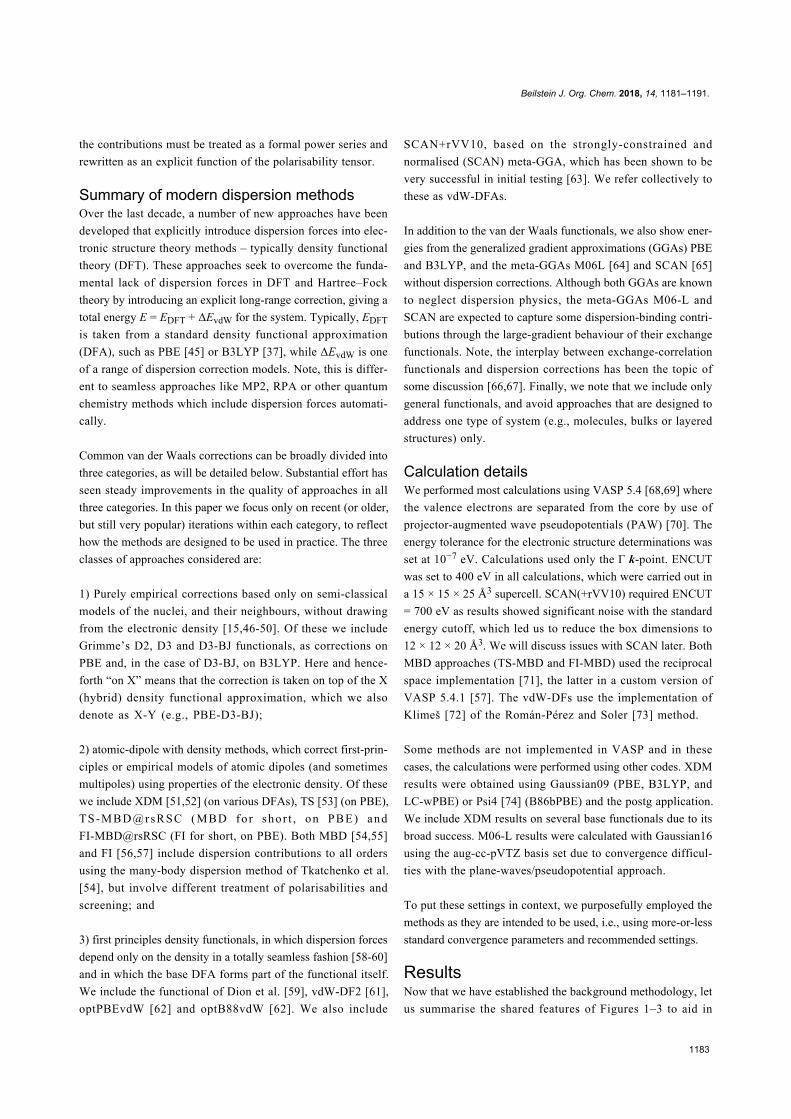
Figure 1: Interaction energies (solid lines) and forces (dashed lines) for the parallel configuration of the benzene dimer. Each panel groups a differentfamily of computational approach. The top row (from left to right) shows GGAs and meta-GGAs without dispersion corrections, and the dimer geome-try. The second row reports Grimme-D variants (l) and TS/MBD variants (r). The bottom row shows XDM on different DFAs (l), and vdW-DFAs (r). Thebenchmark data is always shown in black.

detailed assessment. Each figure is composed of sub-figures

showing results for selected groupings of methods. Each sub-

figure shows as solid lines the benchmark potential energy

curve Ubench and the potential energy curves from the selected

methods Umethod. They also show the benchmark force Fbench,

and the forces for different methods Fmethod, all in dashes. All

energies and forces are reported as functions of distance, either

between the centre of dimers (Figure 1 and Figure 2) or the

sliding distance (Figure 3).

We adopt some steps to ensure all energies and forces are calcu-

lated in the same way, so as to reduce uncontrolled errors from,

e.g., basis set superpositions or pseudopotentials. Firstly, we use

the electronic structure codes to calculate energies E(R) directly.

We then fit E(R) = E∞ – C6/R6 to the last five points of the

parallel configuration data to find E∞, the extrapolated energy

of two monomers, which lets us determine interaction energies

U(R) = E(R) − E∞. We plot U(R) in Figure 1 and Figure 2, and

use the minimum-energy values directly in Table 1 – Figure 3

shows U(R) = E(R) − E(0). Secondly, we obtain all forces by

fitting cubic splines through the energy data, and taking the de-

rivative of the splines.

Figure 1 shows the interaction energy for the parallel configura-

tion of the benzene dimer (labelled P – with D6h symmetry).

Despite having a minimum as a function of distance between

the two centres, this arrangement is unstable as the dimers wish

to slide apart sideways (see later discussion on Figure 3) to

reduce electrostatic effects, such as overlap of the densities of

the monomers and static quadrupole–quadropole interactions,

which make metastable AA graphite ≈0.23 kcal/mol/C less en-

ergetically favourable compared to AB graphite [75]. This

configuration thus involves competition between dispersion

forces, repulsive electrostatic forces, and other exchange and

correlation effects, making it a good test of dispersion correc-

tions.

Beilstein J. Org. Chem. 2018, 14, 1181–1191.

1185

Figure 2: Interaction energies (solid lines) and forces (dashed lines) for the T configuration of the benzene dimer. Panels are the same as in Figure 1.

It is clear from the figure that D2, XDM (all variants), MBD

and FI all give reliable energies across the entire curve. Their

forces are slightly worse, but still within 0.5 kcal/mol/Å of the

reference data at reasonable intermolecular distances. The more

modern Grimme variants fare worse than their older cousin, and

none of the two-point vdW-DFAs work very well at all, for

energies or forces, except near the minima. Indeed, most of the

tested vdW-DFAs give force errors outside equilibrium that are

similar in magnitude to the force itself. A notable exception is

SCAN+rVV10 which is broadly on a par with XDM and TS/FI-

MBD. Somewhat surprisingly, the semi-local meta-GGA M06L

gives an energy curve which is also in broad agreement with the

benchmark, but which fluctuates [76] making the spline-derived

forces less reliable. Other dispersion-free methods are less suc-

cessful, as expected.

Figure 2 then reports the energies for T configuration as a func-

tion of distance (T – with C2v symmetry), which includes the

global minimum for benzene dimer interactions, or at least a

local minimum that is energetically very close to it. Here the

balance of energetic contributions is more strongly skewed to

dispersion, and it is expected that vdW dispersion corrections

should work better than for the parallel configuration shown in

Figure 1.

Indeed, the successful methods for the parallel geometry (XDM,

MBD, FI) seem to work very well here, reproducing the refer-

ence energies and forces to within methodological error of

≈0.1 kcal/mol. The vdW-DFAs perform slightly better than in

the parallel case, as one would hope. D2, however, is quite poor

despite its success in the parallel case and its more modern

cousins are conversely much better. Again, M06L works well.

Here, however, we notice that SCAN shows significant oscilla-

tions around the true curve, which SCAN+rVV10 inherits (to be

discussed later).

Next, Figure 3 reports the potential energy curves for sliding of

parallel benzene molecules relative to one another at a fixed

inter-planar distance D, known as the slipped-parallel configu-

ration (SP – with C2h symmetry). We show results for

Beilstein J. Org. Chem. 2018, 14, 1181–1191.

1186

Figure 3: Interaction energies U(R;D) = E(R;D) − E(0;D) (solid lines) and forces (dashed lines) for the slipped-parallel configuration of the benzenedimer at D = 3.6 Å. Panels are the same as in Figure 1.

D = 3.6 Å, shown relative to their energy in the perfectly

parallel configuration [i.e., U(R;D) = E(R;D) − E(0;D)]. Here

XDM is a stand-out, giving almost perfect agreement with the

benchmarks, thus indicating its ability to simultaneously capture

competing energy contributions. All other methods are much

more successful here than in the previous tests, reflecting their

consistency in reproducing electrostatic effects compared to

dispersion interactions which are more-or-less constant across

the curves. These results are replicated in other tests

(not shown) at D = 3.2, 3.4 and 3.8 Å. Again, the SCAN and

SCAN+rVV10 curves display oscillations.

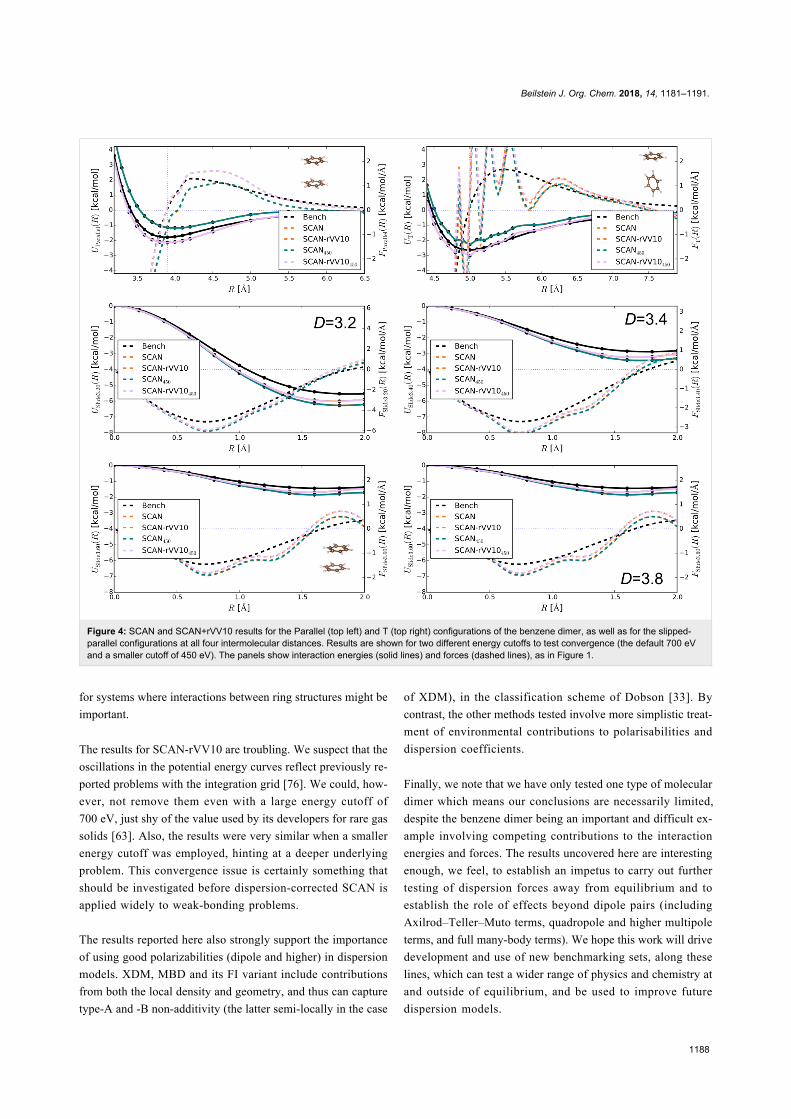
The strange behaviour of SCAN and SCAN+rVV10 warrants

special attention. Previous tests of meta-GGAs using Gaussian-

type orbital codes suggest this issue might be related to the den-

sity of the real-space grid [76]. In Figure 4 we thus show results

for SCAN and SCAN+rVV10 for all four intermolecular dis-

tances (D = 3.2, 3.4, 3.6 and 3.8 Å) and for both the large

energy cutoff 700 eV used in previous calculations, and also a

smaller cutoff of 450 eV.

It is obvious from these curves that the oscillations seem to be

smallest when the overlap between the orbitals is largest, as in

the parallel case and the two closest (D = 3.2, 3.4) sliding cases,

versus the T case and the more distant sliding cases. Further-

more, the oscillations seem to hold consistently for the smaller

and larger energy cutoffs, a result we find somewhat perplexing

as, if they were sensitive to the grid, we would expect

them to decrease with a larger cutoff (and consequently finer

grid).

Finally, in Table 1 we quantify how the different methods

perform in prediction of the relative energies of the various

local minima, U0(T), U0(P) and U0(SP), for the T, parallel (P)

and slipped-parallel (SP) configurations, respectively. We thus

show the energy differences, ΔU(P/SP) = U0(P/SP) − U0(T), be-

tween the local minima for the parallel and slipped-parallel con-

figurations, and the (presumed) global minimum for the T con-

figuration. In all cases we fit quadratic curves to data to obtain a

value as close to the true minimum as possible. We also take

advantage of revised benchmark values from Takatani et al.

Beilstein J. Org. Chem. 2018, 14, 1181–1191.

1187

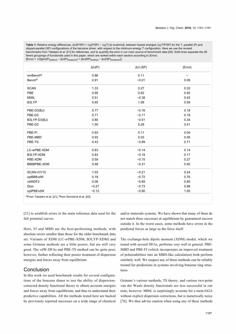
Table 1: Relative energy differences, ΔU(P/SP) = U0(P/SP) − U0(T) [in kcal/mol], between lowest energies U0(T/P/SP) for the T, parallel (P) andslipped-parallel (SP) configurations of the benzene dimer, with respect to the minimum-energy T configuration. Here we use the revisedbenchmarks from Takatani et al. [21] for references, and to quantify the error in our main source of benchmark data [20]. Solid lines separate the dif-ferent groupings of functionals used in this paper, which are ranked within each section according to |Error|.|Error| = 1/2[|ΔU(P)method − ΔU(P)revbench| + |ΔU(SP)method − ΔU(SP)revbench|].

ΔU(P) ΔU (SP) |Error|

revBencha 0.86 0.11 –Benchb 0.91 −0.01 0.09

SCAN 1.33 0.27 0.32PBE 0.95 0.82 0.40M06L 0.51 −0.38 0.42B3LYP 0.65 1.08 0.59

PBE-D3(BJ) 0.77 −0.16 0.18PBE-D3 0.71 −0.11 0.19B3LYP-D3(BJ) 0.80 −0.51 0.34PBE-D2 1.50 0.28 0.41

PBE-FI 0.93 0.11 0.04PBE-MBD 0.93 0.03 0.08PBE-TS 0.43 −0.89 0.71

LC-wPBE-XDM 0.83 −0.14 0.14B3LYP-XDM 0.83 −0.19 0.17PBE-XDM 0.59 −0.15 0.27B86BPBE-XDM 0.48 −0.31 0.40

SCAN-rVV10 1.03 −0.21 0.24optB88vdW 0.18 −0.72 0.76vdWDF2 0.06 −0.69 0.80Dion −0.27 −0.73 0.98optPBEvdW −0.12 −0.90 1.00

aFrom Takatani et al. [21], bfrom Sinnokrot et al. [20].

[21] to establish errors in the main reference data used for the

full potential curves.

Here, FI and MBD are the best-performing methods, with

absolute errors smaller than those for the older benchmark data

set. Variants of XDM (LC-wPBE-XDM, B3LYP-XDM) and

some Grimme methods are a little poorer, but are still very

good. The vdW-DFAs and PBE-TS method can be quite poor,

however, further reflecting their poorer treatment of dispersion

energies and forces away from equilibrium.

ConclusionIn this work we used benchmark results for several configura-

tions of the benzene dimer to test the ability of dispersion-

corrected density functional theory to obtain accurate energies

and forces away from equilibrium, and thus to understand their

predictive capabilities. All the methods tested here are backed

by previously reported successes on a wide range of chemical

and/or materials systems. We have shown that many of them do

not match these successes at equilibrium by guaranteed success

outside it. In the worst cases, some methods have errors in the

predicted forces as large as the force itself.

The exchange-hole dipole moment (XDM) model, which we

tested with several DFAs, performs very well in general. PBE-

MBD and PBE-FI (which incorporates an improved treatment

of polarisabilities into an MBD-like calculation) both perform

similarly well. We suspect any of these methods can be reliably

trusted for predictions in systems involving benzene ring struc-

tures

Grimme’s various methods, TS theory, and various two-point

van der Waals density functionals are less successful in our

tests, however. M06L is surprisingly accurate for a meta-GGA

without explicit dispersion corrections, but is numerically noisy

[76]. We thus advise caution when using any of these methods

Beilstein J. Org. Chem. 2018, 14, 1181–1191.

1188

Figure 4: SCAN and SCAN+rVV10 results for the Parallel (top left) and T (top right) configurations of the benzene dimer, as well as for the slipped-parallel configurations at all four intermolecular distances. Results are shown for two different energy cutoffs to test convergence (the default 700 eVand a smaller cutoff of 450 eV). The panels show interaction energies (solid lines) and forces (dashed lines), as in Figure 1.

for systems where interactions between ring structures might be

important.

The results for SCAN-rVV10 are troubling. We suspect that the

oscillations in the potential energy curves reflect previously re-

ported problems with the integration grid [76]. We could, how-

ever, not remove them even with a large energy cutoff of

700 eV, just shy of the value used by its developers for rare gas

solids [63]. Also, the results were very similar when a smaller

energy cutoff was employed, hinting at a deeper underlying

problem. This convergence issue is certainly something that

should be investigated before dispersion-corrected SCAN is

applied widely to weak-bonding problems.

The results reported here also strongly support the importance

of using good polarizabilities (dipole and higher) in dispersion

models. XDM, MBD and its FI variant include contributions

from both the local density and geometry, and thus can capture

type-A and -B non-additivity (the latter semi-locally in the case

of XDM), in the classification scheme of Dobson [33]. By

contrast, the other methods tested involve more simplistic treat-

ment of environmental contributions to polarisabilities and

dispersion coefficients.

Finally, we note that we have only tested one type of molecular

dimer which means our conclusions are necessarily limited,

despite the benzene dimer being an important and difficult ex-

ample involving competing contributions to the interaction

energies and forces. The results uncovered here are interesting

enough, we feel, to establish an impetus to carry out further

testing of dispersion forces away from equilibrium and to

establish the role of effects beyond dipole pairs (including

Axilrod–Teller–Muto terms, quadropole and higher multipole

terms, and full many-body terms). We hope this work will drive

development and use of new benchmarking sets, along these

lines, which can test a wider range of physics and chemistry at

and outside of equilibrium, and be used to improve future

dispersion models.

Beilstein J. Org. Chem. 2018, 14, 1181–1191.

1189

Supporting InformationWe provide all data generated through this project to allow

other researchers to carry out their own analyses. This file

contains all reference data used for this paper, stored in

comma separated variables format with “#” used to indicate

comments.

Supporting Information File 1All reference data.

[https://www.beilstein-journals.org/bjoc/content/

supplementary/1860-5397-14-99-S1.csv]

AcknowledgementsTG acknowledges support of the Griffith University Gowonda

HPC Cluster. SAT acknowledges funding by the Australian

Government through the Australian Research Council (ARC

DP160101301). Theoretical calculations by TG and SAT were

undertaken with resources provided by the National Computa-

tional Infrastructure (NCI) supported by the Australian Govern-

ment and, for SAT, by the Pawsey Supercomputing Centre

funded by the Australian Government and the Government of

Western Australia. ERJ thanks the Natural Sciences and Engi-

neering Research Council (NSERC) of Canada for financial

support and the Atlantic Computational Excellence Network

(ACEnet) for computing resources.

ORCID® iDsTim Gould - https://orcid.org/0000-0002-7191-9124Erin R. Johnson - https://orcid.org/0000-0002-5651-468XSherif Abdulkader Tawfik - https://orcid.org/0000-0003-3592-1419

References1. Grimme, S. Wiley Interdiscip. Rev.: Comput. Mol. Sci. 2011, 1,

211–228. doi:10.1002/wcms.302. Dobson, J. F.; Gould, T. J. Phys.: Condens. Matter 2012, 24, 073201.

doi:10.1088/0953-8984/24/7/0732013. Grimme, S.; Hansen, A.; Brandenburg, J. G.; Bannwarth, C.

Chem. Rev. 2016, 116, 5105–5154. doi:10.1021/acs.chemrev.5b005334. Woods, L. M.; Dalvit, D. A. R.; Tkatchenko, A.; Rodriguez-Lopez, P.;

Rodriguez, A. W.; Podgornik, R. Rev. Mod. Phys. 2016, 88, 045003.doi:10.1103/RevModPhys.88.045003

5. Hermann, J.; DiStasio, R. A., Jr.; Tkatchenko, A. Chem. Rev. 2017,117, 4714–4758. doi:10.1021/acs.chemrev.6b00446

6. Klimeš, J.; Michaelides, A. J. Chem. Phys. 2012, 137, 120901.doi:10.1063/1.4754130

7. Geim, A. K.; Grigorieva, I. V. Nature 2013, 499, 419–425.doi:10.1038/nature12385

8. Rösel, S.; Quanz, H.; Logemann, C.; Becker, J.; Mossou, E.;Cañadillas-Delgado, L.; Caldeweyher, E.; Grimme, S.; Schreiner, P. R.J. Am. Chem. Soc. 2017, 139, 7428–7431. doi:10.1021/jacs.7b01879

9. Fabrizio, A.; Corminboeuf, C. J. Phys. Chem. Lett. 2018, 9, 464–470.doi:10.1021/acs.jpclett.7b03316

10. Johnson, E. R.; Clarkin, O. J.; Dale, S. G.; DiLabio, G. A.J. Phys. Chem. A 2015, 119, 5883–5888.doi:10.1021/acs.jpca.5b03251

11. Reimers, J. R.; Li, M.; Wan, D.; Gould, T.; Ford, M. J. Non-CovalentInteractions in Quantum Chemistry and Physics; Elsevier, 2017;pp 387–416. doi:10.1016/B978-0-12-809835-6.00015-3

12. Gould, T.; Lebègue, S.; Björkman, T.; Dobson, J. F. In Semiconductorsand Semimetals; Iacopi, F.; Boeckl, J. J.; Jagadish, C., Eds.; 2DMaterials, Vol. 95; Elsevier, 2016; pp 1–33.

13. Goerigk, L. Non-Covalent Interactions in Quantum Chemistry andPhysics; Elsevier, 2017; pp 195–219.doi:10.1016/B978-0-12-809835-6.00007-4

14. Schröder, E.; Cooper, V. R.; Berland, K.; Lundqvist, B. I.;Hyldgaard, P.; Thonhauser, T. Non-Covalent Interactions in QuantumChemistry and Physics; Elsevier, 2017; pp 241–274.doi:10.1016/B978-0-12-809835-6.00009-8

15. Grimme, S.; Ehrlich, S.; Goerigk, L. J. Comput. Chem. 2011, 32,1456–1465. doi:10.1002/jcc.21759

16. Goerigk, L.; Hansen, A.; Bauer, C.; Ehrlich, S.; Najibi, A.; Grimme, S.Phys. Chem. Chem. Phys. 2017, 19, 32184–32215.doi:10.1039/C7CP04913G

17. Tawfik, S. A.; Gould, T.; Stampfl, C.; Ford, M. J. Phys. Rev. Materials2018, 2, 034005. doi:10.1103/PhysRevMaterials.2.034005

18.Řezáč, J.; Riley, K. E.; Hobza, P. J. Chem. Theory Comput. 2011, 7,2427–2438. doi:10.1021/ct2002946

19. Goerigk, L.; Kruse, H.; Grimme, S. ChemPhysChem 2011, 12,3421–3433. doi:10.1002/cphc.201100826

20. Sinnokrot, M. O.; Sherrill, C. D. J. Phys. Chem. A 2004, 108,10200–10207. doi:10.1021/jp0469517

21. Takatani, T.; Hohenstein, E. G.; Malagoli, M.; Marshall, M. S.;Sherrill, C. D. J. Chem. Phys. 2010, 132, 144104.doi:10.1063/1.3378024

22. Lejaeghere, K.; Bihlmayer, G.; Björkman, T.; Blaha, P.; Blügel, S.;Blum, V.; Caliste, D.; Castelli, I. E.; Clark, S. J.; Corso, A. D.;de Gironcoli, S.; Deutsch, T.; Dewhurst, J. K.; Di Marco, I.; Draxl, C.;Dułak, M.; Eriksson, O.; Flores-Livas, J. A.; Garrity, K. F.;Genovese, L.; Giannozzi, P.; Giantomassi, M.; Goedecker, S.;Gonze, X.; Grånäs, O.; Gross, E. K. U.; Gulans, A.; Gygi, F.;Hamann, D. R.; Hasnip, P. J.; Holzwarth, N. A. W.; Iuşan, D.;Jochym, D. B.; Jolle, F.; Jones, D.; Kresse, G.; Koepernik, K.;Küçükbenli, E.; Kvashnin, Y. O.; Locht, I. L. M.; Lubeck, S.;Marsman, M.; Marzari, N.; Nitzsche, U.; Nordström, L.; Ozaki, T.;Paulatto, L.; Pickard, C. J.; Poelmans, W.; Probert, M. I. J.; Refson, K.;Richter, M.; Rignanese, G.-M.; Saha, S.; Scheffler, M.; Schlipf, M.;Schwarz, K.; Sharma, S.; Tavazza, F.; Thunström, P.; Tkatchenko, A.;Torrent, M.; Vanderbilt, D.; van Setten, M. J.; Van Speybroeck, V.;Wills, J. M.; Yates, J. R.; Zhang, G.-X.; Cottenier, S. Science 2016,351, aad3000. doi:10.1126/science.aad3000

23. Hermann, J.; Alfè, D.; Tkatchenko, A. Nat. Commun. 2017, 8,No. 14052. doi:10.1038/ncomms14052

24. Sutton, C.; Risko, C.; Brédas, J.-L. Chem. Mater. 2016, 28, 3–16.doi:10.1021/acs.chemmater.5b03266

25. Zang, L.; Che, Y.; Moore, J. S. Acc. Chem. Res. 2008, 41, 1596–1608.doi:10.1021/ar800030w

26. Neel, A. J.; Hilton, M. J.; Sigman, M. S.; Toste, F. D. Nature 2017, 543,637–646. doi:10.1038/nature21701

27. Jurečka, P.; Šponer, J.; Černý, J.; Hobza, P.Phys. Chem. Chem. Phys. 2006, 8, 1985–1993.doi:10.1039/B600027D

Beilstein J. Org. Chem. 2018, 14, 1181–1191.

1190

28. Lebègue, S.; Harl, J.; Gould, T.; Ángyán, J. G.; Kresse, G.;Dobson, J. F. Phys. Rev. Lett. 2010, 105, 196401.doi:10.1103/PhysRevLett.105.196401

29. Gould, T.; Gray, E.; Dobson, J. F. Phys. Rev. B 2009, 79, 113402.doi:10.1103/PhysRevB.79.113402

30. Gould, T.; Simpkins, K.; Dobson, J. F. Phys. Rev. B 2008, 77, 165134.doi:10.1103/PhysRevB.77.165134

31. Dobson, J. F.; Gould, T.; Vignale, G. Phys. Rev. X 2014, 4,No. 021040. doi:10.1103/PhysRevX.4.021040

32. Misquitta, A. J.; Spencer, J.; Stone, A. J.; Alavi, A. Phys. Rev. B 2010,82, 075312. doi:10.1103/PhysRevB.82.075312

33. Dobson, J. F. Int. J. Quantum Chem. 2014, 114, 1157–1161.doi:10.1002/qua.24635

34. DiStasio, R. A., Jr.; von Lilienfeld, O. A.; Tkatchenko, A.Proc. Natl. Acad. Sci. U. S. A. 2012, 109, 14791–14795.doi:10.1073/pnas.1208121109

35. Ambrosetti, A.; Ferri, N.; DiStasio, R. A., Jr.; Tkatchenko, A. Science2016, 351, 1171–1176. doi:10.1126/science.aae0509

36. Gobre, V. V.; Tkatchenko, A. Nat. Commun. 2013, 4, No. 2341.doi:10.1038/ncomms3341

37. Kim, K.; Jordan, K. D. J. Phys. Chem. 1994, 98, 10089–10094.doi:10.1021/j100091a024

38. Johnson, E. R. J. Chem. Phys. 2011, 135, 234109.doi:10.1063/1.3670015

39. Maurer, R. J.; Ruiz, V. G.; Tkatchenko, A. J. Chem. Phys. 2015, 143,102808. doi:10.1063/1.4922688

40. Christian, M. S.; Otero-de-la-Roza, A.; Johnson, E. R.J. Chem. Theory Comput. 2016, 12, 3305–3315.doi:10.1021/acs.jctc.6b00222

41. Otero-de-la-Roza, A.; Johnson, E. R. J. Chem. Phys. 2013, 138,054103. doi:10.1063/1.4789421

42. Otero-de-la-Roza, A.; DiLabio, G. A.; Johnson, E. R.J. Chem. Theory Comput. 2016, 12, 3160–3175.doi:10.1021/acs.jctc.6b00298

43. Huang, Y.; Beran, G. J. O. J. Chem. Phys. 2015, 143, 044113.doi:10.1063/1.4927304

44.Řezáč, J.; Huang, Y.; Hobza, P.; Beran, G. J. O.J. Chem. Theory Comput. 2015, 11, 3065–3079.doi:10.1021/acs.jctc.5b00281

45. Perdew, J. P.; Burke, K.; Ernzerhof, M. Phys. Rev. Lett. 1996, 77,3865–3868. doi:10.1103/PhysRevLett.77.3865

46. Wu, Q.; Yang, W. J. Chem. Phys. 2002, 116, 515–524.doi:10.1063/1.1424928

47. Wu, X.; Vargas, M. C.; Nayak, S.; Lotrich, V.; Scoles, G.J. Chem. Phys. 2001, 115, 8748–8757. doi:10.1063/1.1412004

48. Grimme, S. J. Comput. Chem. 2006, 27, 1787–1799.doi:10.1002/jcc.20495

49. Grimme, S.; Antony, J.; Ehrlich, S.; Krieg, H. J. Chem. Phys. 2010,132, 154104. doi:10.1063/1.3382344

50. Elstner, M.; Hobza, P.; Frauenheim, T.; Suhai, S.; Kaxiras, E.J. Chem. Phys. 2001, 114, 5149–5155. doi:10.1063/1.1329889

51. Becke, A. D.; Johnson, E. R. J. Chem. Phys. 2007, 127, 154108.doi:10.1063/1.2795701

52. Johnson, E. R. Non-Covalent Interactions in Quantum Chemistry andPhysics; Elsevier, 2017; pp 169–194.doi:10.1016/B978-0-12-809835-6.00006-2

53. Tkatchenko, A.; Scheffler, M. Phys. Rev. Lett. 2009, 102, 073005.doi:10.1103/PhysRevLett.102.073005

54. Tkatchenko, A.; DiStasio, R. A., Jr.; Car, R.; Scheffler, M.Phys. Rev. Lett. 2012, 108, 236402.doi:10.1103/PhysRevLett.108.236402

55. Ambrosetti, A.; Reilly, A. M.; DiStasio, R. A., Jr.; Tkatchenko, A.J. Chem. Phys. 2014, 140, 18A508. doi:10.1063/1.4865104

56. Gould, T.; Bučko, T. J. Chem. Theory Comput. 2016, 12, 3603–3613.doi:10.1021/acs.jctc.6b00361

57. Gould, T.; Lebègue, S.; Ángyán, J. G.; Bučko, T.J. Chem. Theory Comput. 2016, 12, 5920–5930.doi:10.1021/acs.jctc.6b00925

58. Dobson, J. F.; Dinte, B. P.; Wang, J.; Gould, T. Aust. J. Phys. 2000, 53,575–596.

59. Dion, M.; Rydberg, H.; Schröder, E.; Langreth, D. C.; Lundqvist, B. I.Phys. Rev. Lett. 2004, 92, 246401.doi:10.1103/PhysRevLett.92.246401

60. Vydrov, O. A.; Van Voorhis, T. J. Chem. Phys. 2011, 133, 244103.doi:10.1063/1.3521275

61. Lee, K.; Murray, É. D.; Kong, L.; Lundqvist, B. I.; Langreth, D. C.Phys. Rev. B 2010, 82, 081101. doi:10.1103/PhysRevB.82.081101

62. Klimeš, J.; Bowler, D. R.; Michaelides, A. J. Phys.: Condens. Matter2009, 22, 022201. doi:10.1088/0953-8984/22/2/022201

63. Peng, H.; Yang, Z.-H.; Perdew, J. P.; Sun, J. Phys. Rev. X 2016, 6,041005. doi:10.1103/PhysRevX.6.041005

64. Zhao, Y.; Truhlar, D. G. Theor. Chem. Acc. 2008, 120, 215–241.doi:10.1007/s00214-007-0310-x

65. Sun, J.; Ruzsinszky, A.; Perdew, J. P. Phys. Rev. Lett. 2015, 115,036402. doi:10.1103/PhysRevLett.115.036402

66. Pernal, K.; Podeszwa, R.; Patkowski, K.; Szalewicz, K. Phys. Rev. Lett.2009, 103, 263201. doi:10.1103/PhysRevLett.103.263201

67. Hermann, J.; Tkatchenko, A. J. Chem. Theory Comput. 2018, 14,1361–1369. doi:10.1021/acs.jctc.7b01172

68. Kresse, G.; Furthmüller, J. Phys. Rev. B 1996, 54, 11169–11186.doi:10.1103/PhysRevB.54.11169

69. Kresse, G.; Joubert, D. Phys. Rev. B 1999, 59, 1758–1775.doi:10.1103/PhysRevB.59.1758

70. Blochl, P. E. Phys. Rev. B 1994, 50, 17953–17979.doi:10.1103/PhysRevB.50.17953

71. Bučko, T.; Lebègue, S.; Gould, T.; Ángyán, J. G.J. Phys.: Condens. Matter 2016, 28, 045201.doi:10.1088/0953-8984/28/4/045201

72. Klimeš, J.; Bowler, D. R.; Michaelides, A. Phys. Rev. B 2011, 83,195131. doi:10.1103/PhysRevB.83.195131

73. Román-Pérez, G.; Soler, J. M. Phys. Rev. Lett. 2009, 103, 096102.doi:10.1103/PhysRevLett.103.096102

74. Parrish, R. M.; Burns, L. A.; Smith, D. G. A.; Simmonett, A. C.;DePrince, A. E., III; Hohenstein, E. G.; Bozkaya, U.; Sokolov, A. Y.;Di Remigio, R.; Richard, R. M.; Gonthier, J. F.; James, A. M.;McAlexander, H. R.; Kumar, A.; Saitow, M.; Wang, X.; Pritchard, B. P.;Verma, P.; Schaefer, H. F., III; Patkowski, K.; King, R. A.; Valeev, E. F.;Evangelista, F. A.; Turney, J. M.; Crawford, T. D.; Sherrill, C. D.J. Chem. Theory Comput. 2017, 13, 3185–3197.doi:10.1021/acs.jctc.7b00174

75. Leconte, N.; Jung, J.; Lebègue, S.; Gould, T. Phys. Rev. B 2017, 96,195431. doi:10.1103/PhysRevB.96.195431

76. Johnson, E. R.; Becke, A. D.; Sherrill, C. D.; DiLabio, G. A.J. Chem. Phys. 2009, 131, 034111. doi:10.1063/1.3177061

Beilstein J. Org. Chem. 2018, 14, 1181–1191.

1191

License and TermsThis is an Open Access article under the terms of the

Creative Commons Attribution License

(http://creativecommons.org/licenses/by/4.0), which

permits unrestricted use, distribution, and reproduction in

any medium, provided the original work is properly cited.

The license is subject to the Beilstein Journal of Organic

Chemistry terms and conditions:

(https://www.beilstein-journals.org/bjoc)

The definitive version of this article is the electronic one

which can be found at:

doi:10.3762/bjoc.14.99