Embed Size (px)
Citation preview
Economic Policy Sixty-first Panel Meeting
Hosted by the Bank of Latvia Riga, 17-18 April 2015
The organisers would like to thank the Bank of Latvia for their support. The views expressed in this paper are those of the author(s) and not those of the supporting organization.
Are Bank Capital Ratios Pro-Cyclical? New Evidence and Perspectives
Michael Brei (Université Paris Ouest)
Leonardo Gambacorta (Bank for International Settlements)
ARE BANK CAPITAL RATIOS PRO-CYCLICAL? NEW EVIDENCE AND PERSPECTIVES
1
Are bank capital ratios pro-cyclical? New evidence and perspectives
Michael Brei and Leonardo Gambacorta Université Paris Ouest and Bank for International Settlements
SECOND DRAFT – 61st PANEL MEETING OF ECONOMIC POLICY
Please do not circulate or quote without the authors’ permission
SUMMARY
This paper analyses how the new Basel III leverage ratio and risk-weighted regulatory capital ratio behave over the cycle. The analysis proposes a setup to test for the cyclical properties of bank capital ratios, taking into account structural shifts in banks’ behaviour during the global financial crisis and its aftermath. Using a large data set covering international banks headquartered in 14 advanced economies for the period 1995–2012, we find that the Basel III leverage ratio is significantly more countercyclical than the risk-weighted regulatory capital ratio: it is a tighter constraint for banks in booms and a looser constraint in recessions.
We thank Neil Esho, James Haas, Florian Heider, Chunhang Liu, Jing Yang, Davy Reinard, Laurence Scialom, Luca Serafini, Kostas Tsatsaronis and, in particular, the editor Thorsten Beck and two anonymous referees for useful comments and suggestions. We thank Mathias Drehmann and Mikael Juselius for sharing the credit gap data. Gabriele Gasperini and Markus Zoss provided excellent research assistance on QIS data. The views expressed are those of the authors and do not necessarily reflect those of the BIS or the Basel Committee on Banking Supervision. Email addresses: Michael Brei ([email protected]) and Leonardo Gambacorta, corresponding author ([email protected]).
ARE BANK CAPITAL RATIOS PRO-CYCLICAL? NEW EVIDENCE AND PERSPECTIVES
2
1. INTRODUCTION
The main benefit of bank capital requirements is to make the financial system more resilient, reducing the probability of banking crises and their associated output losses. However, the global financial crisis has highlighted the limits of risk-sensitive bank capital ratios (regulatory capital divided by risk-weighted assets (RWA)). Despite numerous refinements and revisions over the last two decades, the weights applied to asset categories seem to have failed to fully reflect banks’ portfolio risk (Acharya and Richardson, 2009; Vallascas and Hagendorff, 2013). To tackle this problem the new regulatory framework of Basel III has introduced a minimum leverage ratio, defined as a bank’s Tier 1 capital over an exposure measure, which is independent of risk assessment (Ingves, 2014).
The aim of the leverage ratio is to act as a complement and a backstop to risk-based capital requirements. It should counterbalance the build-up of a “risk-taking channel” by limiting the effects of risk weight compression during booms (Borio and Zhu, 2012; Adrian and Shin, 2013; Altunbas, Gambacorta and Marques-Ibanez, 2014). Given that the leverage ratio weights all exposures equally and does not depend on estimated default probabilities, it is expected to act counter-cyclically, being tighter in booms when banks increase their activities and looser in busts when they deleverage. Such behaviour of regulatory bank capital over the cycle should produce not only a reduction in the probability of a crisis but also a general reduction in the amplitude of fluctuations in output.1
The Basel III framework requires that the leverage ratio and the more complex risk-based capital requirements work together. On the one hand it is crucial to have risk-sensitive capital constraints in place that require that capital charges are higher for exposures with a low probability of repayment and lower when the probability of repayment of an asset is high. However, since any estimate of a default probability depends on the underlying model assumptions, which may turn to be wrong and lead to risk underestimation, it is important to have, on the other hand, a leverage ratio constraint that is independent of such risk assessments.
1 In our study we consider as pro-cyclical (counter-cyclical) a bank capital ratio that is positively (negatively)
correlated with the cycle. This means that, other things being equal, the ratio tends to increase (decrease) when the economy or financial asset evaluation is growing. The term pro-cyclicality (counter cyclicality) is indeed typically associated in policy discussion with the fact that regulation could magnify (reduce) cycle fluctuations. Along similar lines, Ayuso et al (2004) associate pro-cyclicality with the positive relationship between the capital buffer (regulatory capital minus minimum capital requirements) and real activity. For example, if capital requirements increase in a recession - when building reserves from decreasing profits is difficult or raising fresh capital is likely to be extremely costly - banks would have to reduce their loans and the subsequent credit squeeze would add to the downturn. Our paper differs with respect to Ayuso et al (2004) only with respect to the different bank capital definition (capital ratio vs capital buffer). Adrian and Shin (2010) define pro-cyclical leverage as a positive relation between the change of the ratio total assets over equity (the inverse of the Basel III leverage ratio definition) and the change in total balance sheet size. In this respect, our paper differs in two dimensions: we define the leverage ratio as in Basel III regulation and we focus on the relation with the cycle rather than with bank balance sheet size.
ARE BANK CAPITAL RATIOS PRO-CYCLICAL? NEW EVIDENCE AND PERSPECTIVES
3
In other words, while the risk-based capital requirement refers to a bank’s capacity to absorb potential losses, the leverage ratio indicates the maximum loss that can be covered by equity.2
To our knowledge, this paper provides the first empirical investigation of how the new Basel III leverage ratio behaves over the cycle and how it compares to the risk-weighted regulatory capital ratio. While most existing studies related to our work are focused on either bank leverage (Adrian and Shin, 2010; Laux and Rauter, 2014) or the risk-weighted capital ratio (Kashyap and Stein, 2004; Gordy and Howells, 2006; Saurina and Trucharte, 2007; Repullo, Saurina and Trucharte, 2010) in the context of a single country, we examine the two capital ratios of major banks at the same time and in an international setting. In particular, we shed light on three interrelated questions:
i) Is the new leverage ratio more counter-cyclical (less pro-cyclical) than the risk-sensitive capital ratio?
ii) Has the cyclical sensitivity of bank capital ratios changed when compared across different regulatory regimes?
iii) Are the results different in “normal times” with respect to a crisis period?
Our analysis has to overcome a number of challenges and complications. First, bank-level data are required over a long time period in order to cover (at least ideally) one or more business/financial cycles. Second, we need detailed information on banks’ financial statements to reconstruct the new exposure measure. Third, the cycle indicators have to take into account the macroeconomic environment in which each bank operates. Given that many banks in our sample operate across a wide range of jurisdictions, the cycle indicators have to be weighted according to the location of banks’ assets. And finally, we have to correct for differences in accounting standards among countries when calculating the leverage ratio.
Against these backdrops, in this paper we study the behaviour of the two capital ratios over the cycle using BankScope information on the financial statements of 105 international banks headquartered in 14 advanced economies. The data are available for a long time horizon (1995–2012) that covers various business/financial cycles. However, the BankScope information does not contain all the necessary details to precisely calculate the exposure measure, ie the denominator of the Basel III leverage ratio. More specifically, there are differences in national accounting standards that make international comparisons of leverage ratios difficult. To mitigate this problem, we have used confidential information derived from the Basel Committee’s Quantitative Impact Study (QIS database, BCBS, 2013) to calibrate adjustments for the calculation of a valid proxy for the exposure measure. Finally, to take into consideration
2 The use of a leverage ratio is not new. A similar measure has been in force in Canada and the United States since
the early 1980s (Crawford et al, 2009; D’Hulster, 2009). Canada introduced its leverage ratio in 1982 after a period of rapid leveraging up by its banks, and tightened the requirements in 1991. In the United States, the leverage ratio was introduced in 1981 amid concerns over bank safety due to falling bank capitalisation and a number of bank failures (Wall and Peterson, 1987; Wall, 1989). The introduction of a leverage ratio requirement for large banking groups has been announced in Switzerland in 2009 (FINMA, 2009). Similar requirements have been proposed more recently in other jurisdictions (BCBS, 2014b).

ARE BANK CAPITAL RATIOS PRO-CYCLICAL? NEW EVIDENCE AND PERSPECTIVES
4
the international activity and exposures of the banks in our data set, we weigh macroeconomic variables to map banks’ international operations, using the BIS international banking statistics.
The analysis builds on the econometric model of Ayuso, Pérez and Saurina (2004) allowing in addition for the presence of a structural break in the period 2008–12, which accounts for differences in banks’ capitalisation efforts in response to the crisis and the announcement of the Basel III capital regulation. The structural change analysis allows us to disentangle movements in the leverage ratio that react to changes in normal cycle conditions from those that simply reflect banks’ need to reduce the overall riskiness of their portfolios, or to deleverage in response to the crisis. We investigate the reactivity of different definitions of capital ratios to the cycle (Basel I vs Basel II) by means of sample splits and exploit the heterogeneity in the different regulatory requirements across countries.
Our main results are as follows: (i) In normal times the leverage ratio based on the new exposure measure behaves more counter-cyclical than the risk-weighted capital ratio, in particular when measures for the financial cycle are considered; (ii) The cyclical sensitivity of the capital ratios does not change when we control for different regulatory regimes (Basel I vs Basel II); and (iii) Capital ratios tend to be less counter-cyclical (more pro-cyclical) during the crisis period. The last finding might be explained by the reduced correlation of the denominator (which includes lending) with the cycle measures due to the increased recognition of crisis-related losses or deleveraging practices.
The remainder of the paper is organized as follows. The next section discusses why bank capital regulation is important in making the financial system more resilient and it compares the different Basel regimes from a historical perspective. Section 3 describes the data and some stylized facts on bank capital ratios. Section 4 presents the econometric approach and the main hypotheses we seek to test. Section 5 reports the main results on the behaviour of capital ratios over the cycle. The final section summarizes the main conclusions.
2. WHY IS BANK CAPITAL IMPORTANT? THEORY AND REGULATION
The recent experience with the global financial crisis has highlighted potential weaknesses of the existing framework on capital regulation, and it has stimulated an intense discussion on how to improve the resilience of the banking industry. As we will analyse in more detail below, the Basel III framework introduces a number of significant modifications that are intended to strengthen the efficiency of bank regulation by: (i) reducing the pro-cyclicality of the risk-sensitive capital requirements embedded in Basel II with the use of counter-cyclical capital charges; (ii) reducing the possibility of capital arbitrage (e.g. the shift of investments into asset classes with low-risk weights or the underreporting of risks) by the introduction of a supplementary leverage ratio; and (iii) reducing the possibility of “model error” and the underestimation of risks which goes along with the introduction of the supplementary leverage ratio.

ARE BANK CAPITAL RATIOS PRO-CYCLICAL? NEW EVIDENCE AND PERSPECTIVES
5
2.1 Definition of bank capital and the “moral hazard problem”
Banks finance their activities primarily by deposits, wholesale debt market instruments, securitisation and bank capital. Bank capital is the part of funds that is contributed by the owners or shareholders of banks and it serves them as a cushion to absorb unexpected losses. The Basel Committee on Banking Supervision (2006) defines Total Capital as the sum of Tier 1 or core capital and Tier 2 or supplementary capital. Tier 1 capital consists of equity capital and disclosed reserves (retained earnings), whereas Tier 2 capital might include – depending on the national regulatory framework – undisclosed reserves, revaluation reserves, general provisions, hybrid debt and subordinated term debt.
The main objective of capital regulation is to ensure that banks have sufficient internal resources to withstand adverse economic shocks and to improve incentive distortions that are created by a number of market imperfections. Moral hazard associated with (mispriced) deposit insurance (Merton, 1977) and the perception of implicit government guarantees (Fahri and Tirole, 2012) may leave a bank’s funding cost insensitive to its risk choices and lead a bank to take on more risks than it would otherwise. Another major problem is that banks do not fully take into account the negative externalities their financial distress might pose on the banking sector and the economy as a whole (Allen and Gale, 2000). Such systemic costs include losses absorbed by the deposit insurance, bail-out costs of distressed institutions, or disruptions to other banks and borrowers. The objective of capital regulation is to get banks to internalize the systemic costs associated with bank failures and market stress. By requiring banks to hold a minimum amount of capital, banks have to bear some of the downside risk of their investment decisions which should reduce managers’ incentives to take on excessive risks.
From the perspective of a social planner, the benefits of capital regulation in terms of reducing expected default costs have to be counterweighted by the potential costs (Kashyap and Stein, 2004). More specifically, if it is expensive for banks to hold additional capital, a higher capital requirement will lead to a reduction in the supply of positive net present value loans. In this sense, the objective of optimal capital regulation is to find a balance between two conflicting objectives: (i) protecting the system against costs of bank failures and moral hazard, and (ii) encouraging banks to make positive net present value loans.
2.2 Capital regulation theories: leverage and risk-sensitive capital ratios
Bank regulators have developed over time a sophisticated system of solvency regulations that are aimed at increasing the safety of individual institutions and the stability of the financial system. Although bank regulation differs across countries, it most often encompasses a number of complementary instruments including deposit insurance, capital and liquidity requirements, bank supervision and activity restrictions (Barth, Caprio and Levine, 2013). Since there is no general consensus in the literature about the relative importance and consequences of the market imperfections in the banking sector, there exist competing theories that have different assumptions and conclusions about the optimal regulation of banks (Freixas and Rochet, 1997).
ARE BANK CAPITAL RATIOS PRO-CYCLICAL? NEW EVIDENCE AND PERSPECTIVES
6
The “portfolio approach” of solvency regulation interprets a bank as an agent who manages a portfolio of assets and liabilities. This implies that optimal regulation can be assessed within the portfolio choice theory developed by Markowitz (1952). In this set-up it has been shown that if capital is relatively more costly than other liabilities, then the introduction of a minimum capital ratio may induce banks to increase the expected portfolio return on the back of higher risks – in an attempt to compensate for the increased costs of funding (Kim and Santomero, 1988; Rochet, 1992). Consequently, it has been argued that capital requirements should be sensitive to portfolio risks.
The “incentive approach” of solvency regulation addresses the distortions that arise due to information asymmetries across banks and regulators as a result of deposit insurance. Accordingly, optimal regulation can be assessed within a principal-agent model between the public insurance system and the private bank. The optimal incentive scheme, which induces banks to internalize the costs faced by the deposit insurance fund, can be achieved by a capital requirement that is contingent on a bank’s quality of assets (Giammarino, Lewis and Sappington, 1993; Bensaid, Pagès, and Rochet, 1993).
The “incomplete contract approach” takes into account the fact that the incentives of bank managers and shareholders may diverge, since managers tend to own only a small fraction of bank capital (inside equity). The theoretical models developed by Dewatripont and Tirole (1993, 1994) assume that a manager may improve a bank’s portfolio quality by exerting an effort that is costly and imperfectly observed by outsiders. In this context, the incentives of bank managers can be improved by giving the outsiders control rights over a bank that are contingent on a bank’s performance. Therefore, optimal solvency regulation under this approach complements risk-sensitive capital requirements with contingent control rights.3
The theories just described thus motivate the use of risk-sensitive capital requirements that are subject to some sort of contingency with respect to control rights and the macroeconomic environment. A theoretical contribution suggesting that optimal bank regulation in the form of risk-sensitive capital requirements should be complemented by a risk-independent leverage ratio is that of Blum (2008). Using an adverse selection model with profit-maximizing banks and costly capital, he shows that the effectiveness of risk-sensitive capital requirements depends on the existence of a supplementary leverage ratio. The underlying theory is based on the idea that regulators only have limited ability in verifying banks’ risk assessment ex ante. Since bank managers know that the reporting of higher risks leads to higher capital charges, they might have incentives to understate risk choices. To induce truthful revelation, it is thus necessary that banks are sanctioned ex post, whenever such banks are identified by the regulator. However, as long as the regulator’s ability in identifying underreporting banks is limited, an additional leverage ratio helps to improve banks’ incentives by reducing the
3 More recently, Dewatripont and Tirole (2012) have extended their analysis to include macroeconomic shocks.
They show that optimal capital regulation requires that macroeconomic shocks have to be automatically neutralized to keep the incentives of investors in control unchanged. The results suggest that such an offsetting of aggregate shocks could be achieved by dynamic provisioning, or the imposition of counter-cyclical capital buffers.
ARE BANK CAPITAL RATIOS PRO-CYCLICAL? NEW EVIDENCE AND PERSPECTIVES
7
expected profit of risk underreporting. In other words, a supplementary leverage ratio makes the risk-sensitive capital requirement based on internal rating models incentive compatible.
2.3 Basel regimes and pro-cyclicality
The 1988 Basel Accord (Basel I) was initially adopted by the G-10 with the aim of harmonizing capital regulation across countries and strengthening the stability of the international banking system (BCBS, 1988). The framework was designed to encourage banks to increase their capital positions and to make regulatory capital sensitive to banks’ portfolio risk. Accordingly, assets and off-balance sheet activities were assigned risk weights between 0 and 100 percent according to their perceived risks, and banks were required to hold a minimum of overall capital equal to 8% of their risk-weighted assets. Despite the better alignment of banks’ individual portfolio risk and their regulatory capital charges, the Basel I Accord has shown significant weaknesses which ultimately led to the introduction of the Basel II Accord approved in 2004 and implemented in most industrial countries in 2007. The regulatory reform was based on the argument that the Basel I capital requirements did not allow to differentiate between high and low quality assets in the same risk category, which could induce banks to shift their investments from high to low quality assets in the same risk class and for the same level of required capital.
The primary goal of Basel II was to improve the risk-sensitivity of the Basel I capital requirements (BCBS, 2006). In the Basel II framework, regulatory capital charges are set at the individual loan level and are determined either by a standardised approach that uses (where available) external ratings in the determination of risk weights, or an Internal Ratings Based (IRB) approach with five inputs: the borrower’s one-year probability of default (PD), the expected loss given default (LGD), the remaining maturity (M), the asset-value correlation to account for the dependence of defaults in the portfolio (), and a target, one-year solvency probability (q) for bank (BCBS, 2004; Gordy and Howells, 2006; Panetta et al., 2009; Repullo, Saurina and Trucharte, 2010). While the parameters and q are set by the regulator, banks compute their own PD for each exposure within the foundation IRB approach, and within the advanced IRB approach they estimate in addition the LGD. As compared to the flat capital requirements of the Basel I framework, the Basel II capital requirements should in principle be a more accurate measure of capital adequacy and reduce pricing distortions across different asset categories and thereby improve banks’ risk incentives.
Albeit its potential benefits in terms of a better alignment of portfolio risks and capital charges on a bank-by-bank basis, the Basel II Accord has raised a number of concerns. One particular concern has been that the new capital requirements tend to be pro-cyclical, which means that capital charges decrease when the economy is booming and increase when the economy is in a recession, thereby contributing to business cycle volatility (Allen, 2004; Kashyap and Stein, 2004; Gordy and Howells, 2006; Panetta et al., 2009; Repullo, Saurina and Trucharte, 2010). The argument is that risk-sensitive capital charges will decrease during booms, because during
ARE BANK CAPITAL RATIOS PRO-CYCLICAL? NEW EVIDENCE AND PERSPECTIVES
8
this period typically default risk estimates decrease, while the reverse is observed during busts (Borio, Furfine and Lowe, 2001). To the extent that banks expand (cut back) lending in response, economic expansions (downturns) can be reinforced by capital requirements that depend inversely on borrowers’ default probabilities. The literature has produced different recommendations on how to tackle the pro-cyclicality of the risk-sensitive capital requirements by either smoothing the “inputs” of the IRB approach (the probability of default) or the “output” (the capital charge) by a multiplier that is related to the business cycle (Kashyap and Stein, 2004; Gordy and Howells, 2006; Repullo, Saurina and Trucharte, 2010). The issue of pro-cyclicality of risk-sensitive capital requirements is explicitly addressed in the new Basel III Accord in the form of a counter-cyclical capital buffer that is accumulated on the base of the deviation of the credit-to-GDP ratio from its long-term trend (Gambacorta and Drehmann, 2012).
The introduction of a supplementary leverage ratio under the new Basel III Accord can be seen as a complementary device to tackle the problems associated with the risk-sensitive Basel II capital requirements. One major reason for its introduction was that the leverage ratio is independent of banks’ internal risk models and external borrower ratings. As a consequence, it should counterbalance the build-up of risk by limiting the effects of risk weight compression during booms associated both with improvements in borrower ratings (Kashyap and Stein, 2004; Gordy and Howells, 2006; Repullo, Saurina and Trucharte, 2010) and with the danger of understating risks within the IRB approach (Mariathasan and Merrouche, 2014). The underlying argument is that, other things being equal, the leverage ratio - defined as capital over total assets - will tend to decrease during booms when banks expand their balance sheets. This will make the leverage regulatory minimum a tighter constraint, independent of risk assessment and reporting, and banks with limited capital will be forced either to increase their capital base or to reduce their activities. In other words, a minimum leverage ratio requirement will limit the extent to which balance sheets are leveraged up during booms and restrict excessive balance sheet growth, while providing banks with loss absorbency before the cycle turns.
It is important to note in this context that a leverage ratio applied to investment banks may not have the same properties as one applied to commercial banks. This difference is due to the fact that balance sheets of investment banks are to a large extent composed of trading assets, securities and derivatives that are marked-to-market, as opposed to loans which are reported at fair value and make up the bulk of commercial bank assets. If balance sheets were entirely marked-to-market, then under particular assumptions the leverage ratio might increase during booms when asset prices increase (Adrian and Shin, 2010). For example, let us assume that a bank has 100 dollars of assets that are marked-to-marked, 90 of debt and 10 of equity. If the liability side is assumed to be constant and assets increase to 101 due to an increase in asset prices, then the leverage ratio would increase from 10% (=10/100) to 10.89% (=11/101). Although this arithmetic is very simplistic and assumes that one side of the balance sheet is marked-to-market and the other not, it suggests that it is important that the leverage ratio is defined as an accounting measure based on book values rather than market values.
ARE BANK CAPITAL RATIOS PRO-CYCLICAL? NEW EVIDENCE AND PERSPECTIVES
9
The new Basel III leverage ratio has a number of other attractive features. Given that the leverage ratio treats all exposures equally regardless of their estimated risk, it makes banks and the financial system more resilient to model risk, and risk estimation uncertainty. As the recent experience with the global financial crisis revealed, banks have experienced large losses associated with exposures to products that were seen as very low risk on the basis of their historical record (BoE, 2014). A leverage ratio should therefore provide a greater resilience against events that are neither foreseen by risk models nor by stress tests. The leverage ratio is also a relatively simple measure that accounts for differences in accounting standards across countries, which could make banks more comparable than they would be based on their risk-weighted capital levels or the stress tests. Finally, by definition the Basel III leverage ratio takes explicitly into account the amount of off-balance sheet items in the exposure measure (for details, see Appendix A) and therefore is preferable to a simple accounting leverage ratio with total assets at the denominator and can act as an additional complement to the risk-weighted Basel II capital ratio in reducing the possibility of (accounting) forms of capital arbitrage.
Basel III leverage ratio and the risk-sensitive Basel II capital requirement are two complementary measures of capital adequacy that capture different types of risks. If used in isolation, the leverage ratio’s main strength would also be its main weakness, as it does not take into account differences in the default probabilities of individual assets (BoE, 2014). If the leverage ratio were the only constraint, then banks would be incentivised to invest in high risk assets, since there would be no additional capital charge relative to low risk assets. Indeed, this type of risk-shifting effect is a major reason for having risk-weighted capital requirements in the first place.
In conclusion, while the risk-weighted capital ratio corrects banks’ incentives to shift their investments into riskier assets by charging risk-based capital requirements, the leverage ratio increases banks’ resilience against model risk, risk estimation uncertainty and excessive balance sheet expansion when the measured risk is low.
3. DATA AND STYLISED FACTS ON BANK CAPITAL RATIOS
Bank-level data are obtained from BankScope, a commercial database maintained by International Bank Credit Analysis Ltd (IBCA) and the Bureau van Dijk. We consider consolidated bank statements, in line with the view that the relevant economic unit is the internationally active bank taking decisions on its worldwide consolidated assets and liabilities. This is a natural choice, since capital adequacy is typically measured at the group level. Our sample adopts an annual frequency and includes major international banks. It covers the 18 years from 1995 to 2012, a period spanning different economic cycles, a wave of consolidation, and the global financial crisis.
The sample of banks covers the major financial institutions from the G10 countries, plus those of Austria, Australia and Spain. To ensure consistently broad coverage, we select banks by country in descending order of size to cover at least 80% of the domestic banking system. With
ARE BANK CAPITAL RATIOS PRO-CYCLICAL? NEW EVIDENCE AND PERSPECTIVES
10
this procedure, we identified in total 105 banking institutions that cover over 70% of worldwide banking assets as reported in The Banker magazine on the Top 1,000 banks at end-2008.4 The consolidation of the banking sectors during the last two decades makes it important to control for mergers and acquisitions (M&A). Doing so serves to exclude spurious bursts of individual balance sheet positions that reflect only banks’ reorganisations. In particular, we adjust for 155 mergers and acquisitions over the sample period by constructing pro-forma entities at the bank holding level.5 For each country, Table 1 shows the number of banks in our sample that are headquartered in each jurisdiction, along with their combined asset size and location of clients. The columns on the “location of the ultimate borrower”6 in the table show, unsurprisingly, that banks headquartered in different countries also differ in the level of international activity and exposure, ranging from less than 20% of claims on borrowers outside their home country for Italian and Japanese banks to more than 60% for Swiss banks. It is thus important to adjust our cycle measures for the location of bank assets in the form of a weighted average of the country-specific cycles in which banks operate. Finally, a total of 42 banks have received public recapitalisations during the global financial crisis suggesting that our econometric analysis has to take into account both the crisis and the public bailouts (see Figure 1).
In the analysis we consider two capital ratios: I) The new Basel III leverage ratio (TIER 1/ Total exposure); and II) Capital to Risk-weighted Assets ratio (TIER 1/ Risk-weighted assets). The latter will be analysed under the different definitions of Basel I and Basel II and in relation to existing leverage constraints.
The two ratios have different denominators and relate to different concepts of solvency. Definition I) corresponds to the leverage ratio recently adopted by the Basel Committee on Banking Supervision (BCBS, 2014). A bank’s exposure is defined by the sum of the following components: (a) on-balance sheet exposures; (b) derivative exposures; (c) securities financing transaction (SFT) exposures; and (d) off-balance sheet (OBS) exposures.7 Definition (II) corresponds to the Capital to Risk-weighted Assets ratio (CRAR) and includes at the denominator on balance sheet and off-balance sheet exposures, weighted according to risk based on the regulatory requirements (BCBS, 1988, 2005).
Table 2 reports the two capital ratios by country. A few patterns emerge. First, as expected, the level of the leverage ratio with the exposure measure at the denominator is structurally lower
4 See http://www.thebanker.com/Top-1000-World-Banks.
5 We construct individual bank histories by drawing on the merger and acquisition dates of large banking institutions provided to us by central banks and complemented by Bureau van Dijk’s Zephyr database. Starting with 260 consolidated banking groups, we adjust banks’ financial statements backwards by aggregating the reported positions of the acquirer and the target bank prior to the merger or acquisition. The approach used in this paper for the treatment of mergers has been widely used in the literature. See for example Ehrmann et al (2002), Gambacorta and Mistrulli (2004), and De Haas et al. (2014). As a robustness check, we estimated the regressions for a subset of observations that are not subject to the merger adjustment. The results have been similar in terms of significance and magnitude and they can be obtained from the authors upon request.
6 The concept of “ultimate borrower” is based on the country where the ultimate risk or obligor resides, after taking into account risk transfers. The information for the location of the ultimate borrower is not available at the individual bank level and it has been estimated by merging BankScope data with data from the BIS consolidated international banking statistics.
7 For more information on the calculation of the exposure measure see Appendix A.
ARE BANK CAPITAL RATIOS PRO-CYCLICAL? NEW EVIDENCE AND PERSPECTIVES
11
than the CRAR. This is not surprising, since the exposure is not weighted for risk. Second, leverage ratios vary importantly across countries. The lowest ratios have been reported by banks headquartered in Germany and France (2.9% and 2.5% on average over the period 1995–2012), while US and Spanish banks reported the highest ratios (5.8% and 5.4%, respectively). And third, banks hold on average significant (discretionary) Tier 1 capital in excess of the regulatory minimum of 4% of risk-weighted assets in all countries. Only in very few cases did banks report lower capital ratios than the regulatory minimum.
Cohen and Scatigna (2014) document that capital ratios increased after the Lehman default (September 2008) owing to market discipline effects, public recapitalisations, and the announcement of the introduction of the Basel III capital regulation (December 2009). As indicated in Figure 2, the upward trend in capital ratios is evident for all macro regions, and the trend has been even more pronounced for risk-weighted capital ratios (the shaded area indicates the post-Lehman period). This is consistent with the evidence in Cohen and Scatigna (2014), who find that banks from advanced economies on the one hand increased capital through retained earnings, and on the other reduced their risk-weighted assets relative to total assets in the period 2009–12.
Table 3 slices the data set along three dimensions: global importance (global systemically important banks (GSIBs) vs small banks), asset risk, and profitability. These bank-specific characteristics are controlled for in the econometric exercise (see next section).
We consider the reaction of capital ratios to four cycle indicators:
a) The annual growth rate of nominal GDP (expressed in national currency);
b) The annual growth rate of real GDP;
c) The credit-to-GDP gap (the difference between the credit to GDP ratio and its trend);8
d) The annual growth rate of total credit to the private non-financial sector (expressed in national currency).
The four cycle measures are calculated as a weighted average across the jurisdictions in which banks are active, using foreign claims data from the BIS consolidated banking statistics. The adjustment is intended to control for both domestic and international macroeconomic conditions so that the cycle indicators can capture the macroeconomic conditions in the major countries in which banks operate. Figure 3 shows the distribution of the three bank-specific cycle indicators in the sample. The financial cycle represented by the credit gap and has a lower frequency (longer duration) than the real business cycle.
Table 4 indicates average bank features and business cycles by macro regions. While the risk-weighted capital ratios are quite comparable on average across the regions, the leverage ratios show more heterogeneity, and are lower for banks headquartered in the European region. With
8 Credit-to-GDP gaps are derived, in line with the Basel III guidelines for the counter-cyclical capital buffer, as the
deviations of the credit-to-GDP ratios from their one-sided (real-time) long-term trend. Trends are calculated using a one-sided Hodrick-Prescott filter with a smoothing factor lambda of 400,000, taking account only of information up to each point in time. For more details see Drehmann (2013).
ARE BANK CAPITAL RATIOS PRO-CYCLICAL? NEW EVIDENCE AND PERSPECTIVES
12
regards to our cycle measures, it seems that nominal and real GDP growth rates such as total credit growth are comparable across the regions. In contrast, there are important differences in terms of the credit gap, ie the Asia-Pacific region shows on average a negative credit–to-GDP gap of –4.0%, while the euro area recorded a credit gap of 5.9% over the sample period.
4. THE ECONOMETRIC MODEL
The empirical specification test how capital ratios behave over the cycle. In performing this exercise, we need to differentiate the cyclical properties of the ratios in normal times and during the crisis. We address this problem by including interaction terms between a dummy tC (that takes the value of one in 2008–12 and 0 elsewhere) and the regression variables, thus allowing for a parameter shift in the estimated response depending on the state of the economy. The dummy tC aims at capturing not only the effect of the financial crisis but also changes in banks’ behaviour due to the Basel III regulatory reform and the anticipation of more stringent capital requirements in the future. Following Ayuso et al (2004), we estimate the following dynamic panel regression:
ijtijtijtt
ijttijtttjiijt
IFRSXC
YCLCCL
1*
*1
*
)(
)()( (1)
where ijtL denotes the leverage (or risk-weighted capital) ratio in period t of bank i headquartered in country j. The theoretical framework for the empirical equation (1) with no structural change ( 0tC ) can be derived from a simple model in which a representative bank minimises its intertemporal costs for capital (see Section 2 in Ayuso et al (2004)). The lagged dependent variable ( 1ijtL ) captures short-term adjustment costs that arise due to asymmetric information and rigidities in capital markets which make it difficult to raise capital at short notice in response to negative capital shocks (Myers and Majluf (1984)). The direct costs of remunerating shareholders and the risk profile of the banks are controlled for by means of bank-specific characteristics ( 1ijtX ). The cycle variable ijtY is added in order to determine whether it has an additional effect on the level of capital (the numerator of the ratio ijtL ) or banks’ total activity (its denominator).
The variable j indicates country fixed effects that control for time-invariant differences in regulation and fiscal regimes across countries (Albertazzi and Gambacorta (2010)). Following the recent literature on the capital structure of financial and non-financial firms, we include bank-level fixed effects i, because there exists evidence that capital ratios are to a large extent driven by unobserved time-invariant and institution-specific factors (Lemmon et al, 2008; Gropp and Heider, 2010). The dummy IFRSijt (that takes the value of one once a bank adopted IFRS and 0 elsewhere) takes into account changes in the measurement of certain balance sheet items and other differences in accounting due to the introduction of the International Financial Reporting Standards (IFRS) standards, notably, the rules concerning the offsetting of
ARE BANK CAPITAL RATIOS PRO-CYCLICAL? NEW EVIDENCE AND PERSPECTIVES
13
derivatives on the asset and liability side. Most countries (except Canada, Japan and the United States) changed accounting standards from local Generally Accepted Accounting Practices (GAAP) to IFRS in 2005–06.
As dependent variables ( ijtL ), we consider, one at the time, the two capital ratios described in the previous section: (I) the new Basel III leverage ratio (Tier 1/Exposure measure) and (II) the capital to risk-weighted assets ratio (Tier 1/risk-weighted assets). The cycle indicators ( ijtY ) weighted by the location of the ultimate borrowers are: (a) the annual growth rate of nominal GDP; (b) the annual growth rate of real GDP; (c) the credit-to-GDP gap (the difference between the credit-to-GDP ratio and its trend); and (d) the annual growth rate of total credit to the private non-financial sector.9
The bank-specific characteristics included in the vector 1ijtX are: bank size (log of total assets), asset risk (standard deviation of the annual percentage change in the market value of assets) and bank profitability (return on assets, ROA). These control variables are typically used in studies that explain banks’ choice of target capital ratios, because they tend to capture the direct cost of remunerating capital and the risk profile of the banks (Milne and Whalley (2001), Ayuso et al (2004), Gropp and Heider (2010)).
The direct costs of remunerating capital are measured by bank profits. On the one hand, high profits might reflect the direct cost of remunerating capital, and in this case one should expect a negative relationship with the capital buffer. On the other hand, high profits at t–1 should have a positive relation with capital at t, if they are used to increase capital by retained earnings (Ayuso et al (2004), Heid et al (2004), Gropp and Heider (2010)). Moreover, banks with higher profits should incur lower costs when issuing equity, since they are more likely to distribute dividends in the future. However, the relation between profits and capital during the recent financial crisis might have changed since banks that faced large losses came under more market pressure to strengthen their capital ratios than did other banks.
Banks with a higher risk profile are expected to hold higher levels of capital. Holding capital in excess of the regulatory minimum reduces the probability of failure and therewith expected default costs, which include the loss of charter value and reputational costs (Acharya (1996)). Higher capital levels also reduce the costs arising from non-compliance with regulatory capital requirements (Ayuso et al (2004)). We measure bank risks by the volatility of the market value of assets. The higher the volatility of assets, the less certain investors are about a bank’s value and the more likely a bank can be pushed into default. Therefore, if banks set their capital in line with the riskiness of their portfolios, then the relationship would be positive (Milne and Whalley (2001)). We complement the analysis by using as alternative measure of banks’ risk loan loss provisions (typically backward looking) and expected default frequency (one year ahead).
9 We include capital ratios and the credit gap in levels, while the volume of credit and nominal and real GDP are in
growth rates. Unit root tests confirmed the stationary (I(0)) properties of these variables. The use of stationary variables in the regressions aims at mitigating spurious correlation problems.
ARE BANK CAPITAL RATIOS PRO-CYCLICAL? NEW EVIDENCE AND PERSPECTIVES
14
The variable size could be influenced by the costs of either failure or capital adjustment. In the first case, big banks might be expected to maintain lower buffers, as according to the “too-big-to-fail” hypothesis they believe that in the event of difficulties they will receive support from the regulator (negative correlation). In the second case, large banks may hold larger buffers if they are more complex and, hence, asymmetric information is more important (positive correlation).
There are three main hypotheses that equation (1) seeks to test:
(i) How do leverage and risk-weighted capital ratios react to the business cycle? Do they behave pro-cyclically ( 0 ) or counter-cyclically ( 0 )?
(ii) Has the capital ratios’ sensitivity to the cycle changed when compared across different Basel regimes?
(iii) Have effects (i) and (ii) changed in response to the financial crisis ( 0* )?
One possible identification problem is endogeneity. More specifically it might be argued that the state of the banking sector could also affect the business and credit cycle. We however expect the endogeneity problem to be less important if we consider the business cycle measures as a weighted average of the cycles across the jurisdictions in which banks operate. For example, we can assume that the state of the Swiss banking industry is more important for Switzerland’s economic condition than it is for the US economy, even though Swiss banks also operate in the United States. Moreover, while it is probably true that aggregate leverage conditions could influence the business cycle (Phelan (2014)), the specific amount of leverage at the bank level is less likely to affect the global economic and financial cycle.
To assess the relationship between the leverage ratios and the cycle indicators, we use the generalized method of moments (GMM) estimator for dynamic panel data. We employ the system version of the estimator, because it tends to outperform the difference GMM estimator in terms of consistency and efficiency by the use of both the difference and the levels equation (Blundell and Bond (1998)). As it has been shown by Arellano and Bond (1991) and Blundell and Bond (1998), the coefficient estimates of the two-step system estimator are asymptotically more efficient compared to those of the one-step system estimator. A problem that arises with the two-step estimator however is that the asymptotic standard errors are potentially downward biased, especially when the number of instruments is equal to or larger than the number of cross-sectional units (Beck and Levine (2004)). For these reasons, we employ the two-step version of the system GMM (S-GMM) methodology using in each specification fewer instruments than the number of banks in our sample and by applying Windmeijer’s finite sample correction in the calculation of the two-step covariance matrix (Windmeijer (2005)).
As a final precaution, bank-specific characteristics are lagged by one year (t–1) in order to mitigate a possible endogeneity problem between the bank-specific control variables and the capital ratios. Summary statistics of the specific variables used in the regressions are reported in Table 5.

ARE BANK CAPITAL RATIOS PRO-CYCLICAL? NEW EVIDENCE AND PERSPECTIVES
15
5. RESULTS
The main results are reported in Tables 6–9. Each table is divided into four panels, one for each cyclical indicator ( ijtY ). The S-GMM estimator ensures consistent parameter estimates provided that the differenced error term is not subject to serial correlation of order two (AR(2) test) and that the instruments used are valid (Hansen test). Neither test (as reported at the bottom of each table) should reject the null hypotheses (p-values should be above 0.10).10
Table 6 presents the regression results for equation (1) that aims at capturing the correlation between the cycle and the capital ratios. In particular a negative (positive) sign of the coefficient of the cycle variable ijtY indicates that the leverage/capital ratio is counter-cyclical (pro-cyclical): it decreases (increases) when cycle conditions improve and increases (decreases) when cycle conditions deteriorate.
The main results are the following:
(i) In normal times the new leverage ratio based on the exposure measure is significantly counter-cyclical in all cases, while the risk-weighted capital ratio does not react to real GDP and credit gap movements.
(ii) The two capital ratios tend to be less counter-cyclical (more pro-cyclical) during the crisis period. The different behaviour could depend upon the different shapes of the financial and the real cycles. However, the effect is statistically significant only when the credit gap is considered. This can be due to the fact that the credit gap has taken some time in adjusting after Lehmann’s default because of some persistence in the evolution of credit aggregates. As stressed by Cohen-Cole et al. (2008) bank lending did not drop as much as real activity at the beginning of the global financial crisis because of the use of loan commitments and lines of credit by firms and because of securitization activity returning to banks’ balance sheets.11
A few other interesting results emerge. There is evidence of an important persistence in the capital ratios as indicated by the positive and significant coefficient of the lagged capital ratios, which point to the presence of short-term capital adjustment costs. The analysis of the coefficients on bank-specific characteristics also provides some interesting insights. The positive link between asset risk and capital ratios is in line with the findings in Milne and Whalley (2001), who find evidence that banks set their capital according to the riskiness of their portfolios. The coefficient attached to the size of banks is negative and significant only during normal times in the case of the leverage ratio indicating that, other things being equal, larger banks kept relatively lower buffers as postulated in the “too-big-to-fail” hypothesis
10 The null hypothesis of the AR(2) test is that the errors in the first-differenced equation exhibit no second-order
serial correlation, while the null hypothesis of the Hansen test is that instruments are valid. Failure to reject the null hypotheses of both tests should give support to our estimations.
11 The credit-to-GDP deviation from its long term trend (in short the “credit gap”) is a very good indicator of the increase in the risk of a financial crisis (see Drehmann et al, 2010). Thus in comparison to other variables, it is the best variable for guiding the build-up of a countercyclical capital buffer. However, research also finds that the credit gap does not work well as an indicator for the release phase, once banking crises materialize. On this aspect see also Repullo and Saurina (2010).

ARE BANK CAPITAL RATIOS PRO-CYCLICAL? NEW EVIDENCE AND PERSPECTIVES
16
(Ayuso et al (2004)). The impact of bank profitability on capital ratios in normal times is never positive, indicating the absence of accumulation of capital via retained earnings when controlling for bank risks, size and macroeconomic conditions.
The discussion presented so far has focused on the statistical significance of the coefficients on the cycle indicators. However, also the economic significance is important. For example, given the result in column I of Table 6, a coefficient of –0.060** indicates that, if nominal GDP increases by 4.5% (its annual average growth rate over the sample period equivalent to 1.6 standard deviations), then the leverage ratio drops by 0.27 percentage points on impact (-0.060*4.5) and 1.38 percentage points over the long run (–0.27/(1-0.804)), obtained by imposing the condition that in steady state *
1 LLL ijtijt . Relative to the average leverage ratio of 4.54 percent, this implies a decrease of the leverage ratio of 5.94% (-0.27/4.54) in the short-run and 30.3% (-1.38/4.54) in the long run. Although the coefficient of the leverage ratio associated with the credit gap in column III appears with –0.006* relatively low, an increase of one standard deviation in the credit gap (10.18%) results in a drop of the average leverage ratio of 6.9% over the long-run. Overall, the magnitudes are similar to those obtained by Repullo, Saurina and Trucharte (2010) who suggest that risk-weighted capital requirements should be increased by 6.5% for each standard deviation in GDP growth to neutralise the potential pro-cyclicality of Basel II.
5.1 Different bank types
Next we considered the possibility that the capital ratios of banks of different types (savings and cooperative, non-listed, universal, North American (ie subject to a leverage regulation)) react differently to cycle conditions. To this end, we have included in equation (1) a dummy variable that takes the value of one if a bank is of a specific type and 0 elsewhere (dummy Type). In order to control for the different behaviour of such bank type through the cycle we included interactions between the business cycle indicator and the dummy Type. In particular, we have estimated the following model:
,)()
()(
1****
***1
*
ijtijtjtijttijttijt
ijttijtttjiijt
ypeT IFRSXCYC Type
TypeCLCCL
(2)
Tables 7a and 7b report the coefficients on the cycle measure ( ****** ,,, ) for the leverage ratio and the risk-weighted capital ratio, respectively. The results indicate that the leverage ratio of savings and cooperative banks (28 intermediaries in our sample) is on average less counter-cyclical compared to commercial banks when the financial measures of the cycle are considered. This result is in line with Laux and Rauter (2014) who find that US savings banks tend to increase their leverage by more than commercial banks in response to an expansion in total assets. By contrast, there are no significant differences in the cyclical sensitivity of the risk-weighted capital ratio of these types of banks. Along similar lines, the
ARE BANK CAPITAL RATIOS PRO-CYCLICAL? NEW EVIDENCE AND PERSPECTIVES
17
leverage ratio of non-listed banks is less counter-cyclical with respect to the financial cycle (which is not surprising as most savings banks are also not listed). Finally, we do not find evidence that the leverage ratios of universal banks (those intermediaries in the last quartile of the distribution of non-interest income over total income) and North American banks are more counter-cyclical compared to those of the other banks.
5.2 Comparing capital regulation regimes
In this section we seek to test whether the cyclical sensitivity of the capital ratios depends on the regulatory regime. There are two potential sources of heterogeneity: (i) the shift from Basel I to Basel II, and (ii) the presence of an additional leverage ratio requirement. As discussed in Section 2, the Basel I regulation has been adopted in 1988 by all countries in our sample. Most of them adopted the Basel II framework in 2007, except for Australia where it was introduced in 2008 and the United States where it was not implemented. A leverage ratio requirement, on top of the risk-weighted capital regulation, has only been in place in Canada and the United States over the entire sample period. We thus augment our baseline specification (1) by including indicator variables for the different regulatory regimes. More specifically, in the regressions on the leverage ratio we include a dummy variable leverage regulation that is equal to one in Canada and the United States and zero otherwise (dropping the country fixed effects for these countries). We then let interact this variable with our cycle indicators and allow for a shift in the estimated response across normal and crisis times. As for the introduction of the Basel II framework, we include a dummy variable Basel II in the regressions on the risk-weighted capital ratio and its interaction with the cycle measure. Given that Basel II was introduced in 2007 in most countries and that the crisis erupted only one year later, it is likely that any potential cyclical effects of Basel II are confounded with the effects captured by our cycle-crisis interaction. We therefore do not include a crisis interaction of the Basel II indicator and the cycle variables.
The estimation results shown in Table 8 suggest that our main results do not change qualitatively. There is some evidence that the Basel III leverage ratio has been higher in countries where a leverage regulation has been in place (having in mind that those regulations were based on a different definition of the leverage ratio) as indicated by the positive coefficient associated with the variable leverage regulation. However, it appears that the cyclical sensitivity of the leverage ratio is not significantly affected by the fact that a minimum leverage ratio requirements was actually in place. As for the results for Basel II, there is weak evidence that the level of the risk-weighted capital ratio decreased in response to its introduction. However, even in this case the correlation between the risk-weighted capital ratio and the cyclical indicators remains unaffected.

ARE BANK CAPITAL RATIOS PRO-CYCLICAL? NEW EVIDENCE AND PERSPECTIVES
18
5.3 The effect of regulatory constraints
Next we considered possible differential impacts due to public recapitalisations during the financial crisis period and the existence of regulatory constraints on specific banks. To this end, we have included in the baseline equation (1) two additional controls: (i) a dummy variable that takes the value of one if a bank had public capital on its balance sheet in any given year and 0 elsewhere (dummy Rescued); and (ii) a dummy variable that takes the value of one if a bank’s regulatory capital buffer, the difference between the regulatory capital ratio and the regulatory minimum, is in the lowest decile of the distribution (dummy onstrainedC ).12
In addition, we allowed for a different behaviour of capital-constrained banks through the cycle. There is evidence that banks might have incentives to increase capital buffers when they are close to the regulatory minimum to avoid costly recapitalisations in times of distress, while unconstrained banks tend to maintain their levels of capital (Jackson et al (1999), Heid et al (2004), Gropp and Heider (2010)). This suggests that the response of the capital ratios to the cycle might be asymmetrical and depend on whether or not a bank is subject to regulatory pressure. The model was therefore further enriched by including interactions between the business cycle indicator and the dummy Constrained. In particular we have estimated the following model:
,)()
()(
1******
*1
*
ijtijtijtjt
ijttijttijtijt
tijtttjiijt
onstrainedC Rescued IFRS
XCYC onstrainedConstrainedC
CLCCL
(3)
The results presented in Table 9 indicate that, after controlling for these effects, the counter-cyclical behaviour of capital ratios is even reinforced. The new definition of the leverage ratio is counter-cyclical in all cases and coefficients are more significant. Interestingly, the risk-weighted capital ratio of capital constrained banks increases with the cycle in normal times, while their leverage ratio does not. This might suggest that banks subject to regulatory pressure increase their regulatory capital ratio by decreasing risk-weighted assets rather than increasing the capital base or deleveraging. In other words, it appears that capital constrained banks shift their activities from assets with a higher risk weight to those that bear a lower risk weight.
As expected, the coefficient of the Rescue dummy is positive but less significant in the case of the risk-weighted capital ratio, while it is strongly significant in the case of the leverage ratio. This result could indicate that rescue packages may not have translated directly into a greater risk-weighted level of capitalisation because of the re-pricing of risks in response to the
12 We consider a bank as capital-constrained when the distance of a bank’s capital ratio from the regulatory minimum
is lower than the 10th percentile of the distribution of distances, taking into account regulatory differences across countries. While all countries have minimum requirements for risk-weighted capital ratios (for Basel I: Tier 1/RWA > 4%, total capital/RWA >8%), additional limits were imposed on banks’ leverage ratios in Canada and the United States (Barth et al (2013)). Constrained banks have, on average, a Basel III leverage ratio of 3.4% and a Tier 1/RWA of 6.3%, while for unconstrained banks the ratios are, respectively, 4.8% and 9.6%. For more information see Appendix B.
ARE BANK CAPITAL RATIOS PRO-CYCLICAL? NEW EVIDENCE AND PERSPECTIVES
19
financial crisis. This result is also consistent with Brei, Gambacorta and von Peter (2013) who find evidence that recapitalisations did not translate into greater credit supply until bank balance sheets were sufficiently strengthened.
5.4 Alternative measures of the cycle and bank risk
An additional test was to consider the response of the leverage and risk-weighted capital ratios to other cycle indicators. More specifically we examined whether the two measures of capital adequacy react to World GDP, housing prices and total credits granted to households only. As shown in Table 10, it appears that the leverage ratio is negatively correlated with the global cycle, while the risk-weighted ratio does not react significantly. On the other hand, the two capital ratios appear to decrease when housing prices and the volume of household credits (mainly mortgages and consumer credits) increase.
We also examined the robustness of our results to the inclusion of other bank-specific risk indicators, namely, banks’ expected default frequency over a one year horizon. The last two columns of Table 10 indicate that our main results are robust to the definition of bank risk. Similar results (not reported for the sake of brevity, but available in the working paper version of this article) are obtained when considering loan loss provisions as a (backward looking) bank risk indicator.
5.5 Basel III leverage ratio vs accounting leverage ratio
So far the analysis has compared the ratio of Tier1 capital over total exposure, and the ratio of Tier1 capital over risk-weighted assets. Given that the denominator of these two ratios differs along two dimensions (the inclusion of derivatives exposures and securities transaction financing exposures versus the use of risk-weights), it is interesting to check whether the different degrees of cyclicality is driven by the broader exposure measure, or by time-varying risk-weights. To better understand the economic forces behind the results, we have run similar regressions using the ratio of Tier1 capital over total (unweighted) assets as a third dependent variable. The results reported in Table 11 indicate that the accounting leverage ratio (TIER1 over total assets) is less counter-cyclical than the Basel III leverage ratio (TIER1 over total exposure). This finding suggests that it is important to account for banks’ off-balance sheet activities, which are not explicitly reflected in the simple accounting leverage ratio. In other words, it is important to take into account off-balance sheet exposures in the calculation of a total exposure measure, since this precaution reduces the possibility of capital arbitrage related to increases in capital ratios by a shift of activities off-the-balance sheet (Jackson et al., 1999; Allen, 2004).
ARE BANK CAPITAL RATIOS PRO-CYCLICAL? NEW EVIDENCE AND PERSPECTIVES
20
5.6 Disentangling the effects on the numerator and denominator
As capital ratios may be changed by altering either the numerator or the denominator, as a further test we tried to disentangle the effects on the Tier 1, the exposure measure, and risk-weighted assets. While Tier 1 capital can be adjusted by retained earnings or issuing equity, the denominators can be modified by, for example, reducing the volume of exposures, securitising loans or shifting into assets that bear a relatively low risk weight such as under Basel I residential mortgages, short-term interbank exposures or government securities (Dahl and Shrieves (1990), Jackson et al (1999), Heid et al (2004)). The way banks adjust the components of their capital ratios is, of course, likely to depend on the business cycle. While, during booms, banks might find it easier to raise capital, during recessions they might prefer to adjust their asset portfolio. The higher the correlation of the denominator with the cycle, the tighter the corresponding regulatory ratio becomes in a boom and the looser it becomes in a bust. As these variables taken in logs turned out to be non-stationary, we used a model in growth rates to avoid the problem of spurious regressions.13 We used the same specification as in equation (1), where the entire set of control variables is interacted with the structural break dummy tC . As a precaution, having a growth rate as dependent variable (where banks’ assets at t–1 are involved), we replaced the variable for bank size measured by the logarithm of assets with dummy variables for GSIBs and SMALL banks to capture the size effect.
The results are presented in Table 12.14 A few patterns emerge. In normal times, the growth rate of Tier 1 capital is not correlated with our cycle indicators.15 This finding indicates that banks do not increase their capital holdings when the economy is booming and tend to smooth capital consumption in recessions (possibly by means of capital injections). On the other side, banks increase their total exposures and risk-weighted assets when business and financial conditions improve. Taken together, these findings indicate that banks increase their activities without accumulating sufficient capital in good times. From another perspective, the results are consistent with pro-cyclicality of leverage (Adrian and Shin, 2010; Laux and Rauter, 2014). The correlation of the denominator and the cycle indicators is somewhat lower during the crisis period, which might be explained by the effect of a sharp reduction in the value of loans and other investments. Finally, the exposure measure is always more reactive to cycle movements with respect to risk-weighted assets which is in line with our previous results on the higher cyclical sensitivity of the leverage ratio.
13 We have calculated growth rates net of valuation effects due to exchange rate movements (see Brei, Gambacorta
and von Peter, 2013). We reduce this potential bias by converting each bank’s item to constant US dollars, using the currency composition of bank assets for banks headquartered in the respective country, as estimated from the BIS international banking statistics. The growth series used in the estimations are thus partially purged of exchange rate-driven contractions and expansions.
14 Note that the lagged dependent variable is not statistically significant in most specifications. To test whether our results are robust to the exclusion of the autoregressive part, we re-estimated the regressions using the fixed effects estimator. The results (not reported for the sake of brevity) are qualitatively similar.
15 The results do not change if we adjust the Tier 1 measure to consider the new (more conservative) definition of capital adopted in Basel III (the correction for the new definition of Tier 1 is discussed in Appendix A.).
ARE BANK CAPITAL RATIOS PRO-CYCLICAL? NEW EVIDENCE AND PERSPECTIVES
21
5.7 Analysing the cyclical properties of the different components of total exposure
As an additional test, we investigated which of the different components of the exposure measure is more correlated with the cycle indicators. In doing so, we divided the exposure measure in five parts: a) loans; b) total securities and on-balance sheet derivatives, c) guarantees, d) other off-balance sheet items (exposure related to securitisation, acceptances and documentary credits, credit commitments); and e) a residual category. We then estimated regressions similar to those reported in Table 12 considering as dependent variable, one at the time, the annual growth rate of each one of the components a) to e) described above. The results are summarized in Table 13 which for the sake of brevity only reports the coefficients of the cycle measures Y(t) and their interactions with the crisis dummy Y(t)*C.
Loans, guarantees and off balance sheet items tend to be positively correlated with both business and financial measures of the cycle. It thus appears that bank exposure during normal times is mainly driven by banks’ lending activity on the balance sheet and off-balance sheet activities that are possibly related to the lending business. On the contrary, securities holdings and on-balance sheet derivatives tend to be negatively correlated with the cycle measures (albeit only significantly in the case of nominal GDP and credit growth) which could indicate to the presence of potential reallocation effects that depend on the economic situation. In other words, banks might have shifted their activities from relatively low-yielding securities towards more profitable lending activities to finance investment projects in good times (Gambacorta, 2004).
5.8 Market based vs accounting based measures
As discussed in Section 2, it would be interesting to evaluate the cyclical behaviour of a capital ratio that is based on market-based measures. Market values of assets tend to be more volatile compared to book values and one may ask whether it is preferable to have minimum requirement based on book or market values. Adrian and Shin (2010) suggest that fair value accounting plays an important role in the cyclicality of leverage, while Amel-Zahed et al (2014) are opposed this view. In particular, if assets are valued at current market prices and liabilities are booked at face values, then accounting equity will be subject to large fluctuations (Greenlaw et al, 2008; Sinn et al, 2011). In the extreme, ie when the majority of assets are market-to-market and liabilities are recorded at book values, then the leverage ratio would tend to increase during booms when asset prices increase. Along similar lines Repullo, Saurina, and Trucharte (2010) argue that the concerns about the cyclicality of the Basel II capital regulation would be exacerbated by mark-to-market accounting by increasing the cyclical movements in bank capital.
Following this debate, we have calculated a market-based measure of the capital ratio using data on 73 listed banks in our sample. In particular the ratio is defined as the market value of banks’ equity (equal to the share price multiplied by the number of shares outstanding) over the

ARE BANK CAPITAL RATIOS PRO-CYCLICAL? NEW EVIDENCE AND PERSPECTIVES
22
market value of banks’ assets. As one can see from Figure 4 the market-based capital ratio is much more volatile compared to the leverage ratio and the RWA capital ratio.
Table 14 presents the results of the regressions that use as the dependent variable our market-based measure of the capital ratio. The main finding is that such a measure is pro-cyclical, as opposed to the new Basel III leverage ratio and the risk-weighted capital ratio. In other words, the market-based leverage ratio increases with the business cycle measures during normal times, whereas there is no evidence of a significant relation with the two financial cycle measures. This finding supports the view that book value measures of the capital ratio are preferable to mitigate pro-cyclicality issues.
6. CONCLUSIONS
This paper tries to provide an answer to three questions: i) Is the new leverage ratio more counter-cyclical (less pro-cyclical) than the capital to risk weighted assets ratio? ii) Has bank capital ratios’ pro-cyclicality changed comparing different Basel regimes? iii) Are results different in “normal times” with respect to a crisis period?
To this end, we compared the new definition of the leverage ratio using the exposure measure as the denominator with the capital-to-risk-weighted assets ratio. To account for banks’ international activity, we have calculated business cycle measures for each bank as a weighted average across the jurisdictions in which the bank operates, using foreign claims data from the BIS international banking statistics.
The analysis has been conducted with bank-level data over the period 1995–2012, for which we reconstructed the new exposure measure using corrections at the country level derived from the QIS database. The main results are the following: (i) In normal times the new leverage ratio based on the exposure measure is always more countercyclical (less pro-cyclical) than the RWA ratio, in particular when measures for the financial cycle are considered; (ii) the cyclical sensitivity of the capital ratios do not change comparing Basel I and the few years of applications of Basel II); and (iii) All capital ratios tend to be less countercyclical (more pro-cyclical) during the crisis period, especially when the credit gap indicator is considered. This might be explained by the reduced correlation of the denominator (which includes lending) with cyclical measures due to the recognition of losses or deleveraging practices.
REFERENCES
Acharya, S (1996): “Charter Value, Minimum Bank Capital Requirement and Deposit Insurance Pricing in Equilibrium”, Journal of Banking and Finance, Vol. 20(2), pp. 351-375.
Acharya, V and Richardson, M (2009): “Causes of the financial crisis”, Critical Review, Vol. 21, pp. 195–210.
Adrian, T and Shin, H S (2010): “Liquidity and Leverage.” Journal of Financial Intermediation, Vol. 19, pp. 418-437.
ARE BANK CAPITAL RATIOS PRO-CYCLICAL? NEW EVIDENCE AND PERSPECTIVES
23
Adrian, T and Shin, H S (2013): “Procyclical Leverage and Value-at-Risk", Review of Financial Studies, vol 27 (2), pp 373-403.
Albertazzi, U and L Gambacorta (2009): “Bank profitability and the business cycle”, Journal of Financial Stability, vol 5, no 4, pp 393–409.
Allen, F and D Gale (2000): “Financial Contagion”, Journal of Political Economy, vol 108, pp 1-33. Allen, L (2004): “The Basel Capital Accords and International Mortgage Markets: A Survey of the
Literature”, Financial Markets, Institutions & Instruments, Vol. 13, No. 2, pp. 41-108. Altunbas, Y, L Gambacorta and D Marques-Ibanez (2014): “Does monetary policy affect bank risk?”,
International Journal of Central Banking, vol 10, no 1, pp 95–135. Amel-Zadeh, A, M E Barth, and W R Landsman (2014): “Procyclical Leverage: Bank Regulation or Fair
Value Accounting?”, Rock Center for Corporate Governance, Working Paper No. 147 Arellano, M and S Bond (1991): “Some tests of specification for panel data: Monte Carlo evidence and an
application to employment equations”, Review of Economic Studies, vol 58, no 2, pp 277–97. Ayuso, J, D Pérez and J Saurina (2004): “Are capital buffers pro-cyclical? Evidence from Spanish panel
data”, Journal of Financial Intermediation, vol 13, pp 249–64. Barth, J, G Caprio and R Levine (2013): “Bank regulation and supervision in 180 countries from 1999 to
2011”, Journal of Financial Economic Policy, vol 5, no 2, pp 111–219. Bank of England (2014): “The Financial Policy Committee's review of the leverage ratio”, October,
www.bankofengland.co.uk/financialstability/Documents/fpc/fs_lrr.pdf. Basel Committee on Banking Supervision (1988): “International convergence of capital measurement and
capital standards”, July, www.bis.org/publ/bcbs04a.pdf. ——— (2005): “International convergence of capital measurement and capital standards: A revised
framework”, November, www.bis.org/publ/bcbs118a.pdf. ——— (2013): “Instructions for Basel III monitoring”, www.bis.org/bcbs/qis/
biiiimplmoninstr_aug13.pdf. ——— (2014a): “Basel III leverage ratio framework and disclosure requirements”,
www.bis.org/publ/bcbs270.pdf. ——— (2014b): “Seventh progress report on adoption of the Basel regulatory framework”,
www.bis.org/publ/bcbs290.pdf. Beck and Levine (2004): “Stock Markets, Banks, and Growth: Panel Evidence”, Journal of Banking and
Finance, vol 28. Bensaid, B, H Pages, and J-C Rochet (1993): “Efficient regulation of banks’ solvency”, Institut
d’Economie Industrielle, Toulouse, France. Mimeo. Blum, J. (2008): “Why ‘Basel II’ may need a leverage ratio restriction”, Journal of Banking & Finance,
Vol. 32, pp. 1699-1707. Blundell, R and S Bond (1998): “Initial conditions and moment restrictions in dynamic panel data
models”, Journal of Econometrics, vol 87, no 2, pp 115–43. Borio, C and H Zhu (2014), “Capital regulation, risk-taking and monetary policy: A missing link in the
transmission mechanism?”, Journal of Financial Stability, vol 8, no 4, pp 236–251. Brei, M and L Gambacorta (2014): “The leverage ratio over the cycle”, BIS Working Papers, no 471. Brei, M, L Gambacorta and G von Peter (2013): “Rescue packages and bank lending”, Journal of Banking
and Finance, vol 37, no 4 (also published as BIS Working Papers, no 357, November 2011). Cohen, B and M Scatigna (2014), “Banks and capital requirements: channels of adjustment”, BIS Working
Papers, no 443. Crawford, A, C Graham and E Bordeleau (2009): “Regulatory constraints on leverage: the Canadian
experience”, Financial System Review, Bank of Canada, June. Dahl, D and R Shrieves (1990): “The impact of regulation on bank equity infusions”, Journal of Banking
and Finance, vol 14, pp 1209–28. De Haas, R, Y Korniyenko, A Pivovarsky, and T Tsankova (2014): “Taming the herd? Foreign banks, the
Vienna Initiative and crisis transmission”, Journal of Financial Intermediation, forthcoming

ARE BANK CAPITAL RATIOS PRO-CYCLICAL? NEW EVIDENCE AND PERSPECTIVES
24
Dewatripont, M and J Tirole (1993): “Efficient governance structure: Implications for banking regulation”, in Capital markets and financial intermediation, editors C. Mayer and X. Vives, Cambridge University Press.
——— (1994): “The prudential regulation of banks”, MIT Press. ——— (2012): “Macroeconomic Shocks and Banking Regulation”, Journal of Money, Credit and
Banking, vol 44, pp 237-254. Drehmann, M (2013): "Total credit as an early warning indicator for systemic banking crises", BIS
Quarterly Review, June. Drehmann, M, C Borio, L Gambacorta, G Jimenez and C Trucharte (2010): “Countercyclical capital
buffers: exploring options”, BIS Working Papers, no 317. D’Hulster, K (2009): “The leverage ratio”, The World Bank Group, Financial and Private Sector
Development Vice Presidency, Note Number 11. Ehrmann, M, L Gambacorta, J Martinez Pagés, P Sevestre and A Worms (2003): “Financial systems and
the role of banks in monetary policy”, in Angeloni I, A Kashyap and B Mojon (eds.), Monetary policy transmission in the euro area, Cambridge University Press.
Farhi, E and J Tirole (2012): “Collective Moral Hazard, Maturity Mismatch, and Systemic Bailouts”, American Economic Review, vol 102, pp 60-93.
FINMA – Swiss Financial Market Supervisory Authority (2009): “New capital adequacy requirements in Switzerland applicable for large banks: Higher capital ratio targets and leverage ratio”.
Fitch Ratings (2009): “A universal spreadsheet for bank analysis”, Global Special Report. Freixas, X and J-C Rochet (1997): “Microeconomics of Banking”, MIT Press Books. Gambacorta, L., and D. Marques-Ibanez. 2011. “The Bank Lending Channel: Lessons from the Crisis.”
Economic Policy 26 (66), pp. 135–182. Gambacorta, L and P Mistrulli (2004): “Does bank capital affect lending behavior?”, Journal of Financial
Intermediation, 13(4), pp 436–57 Giammarino R M, T R Lewis and D Sappington (1993): “An Incentive Approach to Banking Regulation”,
Journal of Finance, vol 48, pp 1523-1542. Greenlaw, D, Hatzius, J, Kashyap, A K and H S Shin (2008): “Leverage Losses: Lessons from the
Mortgage Market Meltdown”, US Monetary Policy Forum Report No. 2. Gordy, M B and B Howells (2006): “Procyclicality in Basel II: Can we treat the disease without killing
the patient?”, Journal of Financial Intermediation, Vol. 15, pp. 395-417. Gropp, R and F Heider (2010): “The determinants of bank capital structure”, Review of Finance, vol 14,
pp 587–622. Heid, F, D Porath and S Stolz (2004): “Does capital regulation matter for bank behaviour? Evidence for
German savings banks”, Discussion Paper Series 2: Banking and Financial Studies, no 3/2004, Deutsche Bundesbank.
Ingves, S (2014): “Banking on leverage”, keynote address to the 10th Asia-Pacific High-Level Meeting on Banking Supervision, Auckland, New Zealand, 25–27 February.
Jackson, P (1999): “Capital requirements and bank behaviour: the impact of the Basel Accord”, Working Paper, no 1, Basel Committee on Banking Supervision.
Jokipii, J and A Milne (2008): “The cyclical behaviour of European bank capital buffers”, Journal of Banking and Finance, vol 32, pp 1440–51.
Kashyap, A K and J C Stein (2004): “Cyclical implications of the Basel II capital standards”, Federal Reserve Bank of Chicago, Economic Perspectives.
Kim, D and A M Santomero (1988): “Risk in banking and capital regulation”, Journal of Finance, vol 43, pp 1219-1233.
Laux, C and T Rauter (2014): “Procyclicality of US Bank Leverage” Mimeo. Lemmon, M, M Roberts and J Zender (2008): “Back to the beginning: Persistence and the cross-section of
corporate capital structure”, Journal of Finance, vol 63, no 4, pp 1575–608. Markowitz, H (1952): “Portfolio Selection”, Journal of Finance, vol. 7, pp 77-91.
ARE BANK CAPITAL RATIOS PRO-CYCLICAL? NEW EVIDENCE AND PERSPECTIVES
25
Mariathasan, M and O Merrouche (2014): “The manipulation of Basel risk-weights Journal of Financial Intermediation, Vol. 23, pp. 300-321.
Merton, R C (1977): “An analytic derivation of the cost of deposit insurance and loan guarantees An application of modern option pricing theory”, Journal of Banking and Finance, vol 1, pp 3-11.
Milne, A and A Whalley (2001): “Bank capital regulation and incentives for risk-taking”, Cass Business School Research Paper.
Myers, S and N Majluf (1984): “Corporate financing and investment decisions when firms have information that investors do not have”, Journal of Financial Economics, vol 13, no 2, pp 187–221.
Repullo, R, Saurina, J, and C Trucharte (2010): “Mitigating the pro-cyclicality of Basel II“ Economic Policy, pp. 659-702, October 2010.
Phelan, G (2014): “Financial intermediation, leverage, and macroeconomic instability”, mimeo, Yale University.
Rochet, J-C (1992): “Capital requirements and the behaviour of commercial banks”, European Economic Review, vol 36, pp 1137-1170.
Saurina, J and C Trucharte (2007): “An Assessment of Basel II Procyclicality in Mortgage Portfolios.“ Journal of Financial Service Research, Vol 32, pp. 81-101.
Sinn, H W, T Buchen, and T Wollmerhäuser (2011): "Trade imbalances - Causes, consequences and policy measures: IFO's statement Camdessus Commission", CESifo Forum 1/2011.
Vallascas, F and J Hagendorff (2013): “The risk sensitivity of capital requirements: Evidence from an international sample of large banks”, Review of Finance, vol 17, pp 1947–1988.
Wall, L D (1989): “Capital Requirements for Banks: A Look at the 1981 and 1988 Standards.” Federal Reserve Bank of Atlanta, Economic Review 74, pp. 14-29.
Wall, L D and D Peterson (1987): “The effect of capital adequacy guidelines on large bank holding companies”, Journal of Banking and Finance, vol 11, pp 581–600.
Windmeijer, F. (2005): “A finite sample correction for the variance of linear efficient two-step GMM estimators”, Journal of Econometrics, Vol. 126, pp. 25-51.
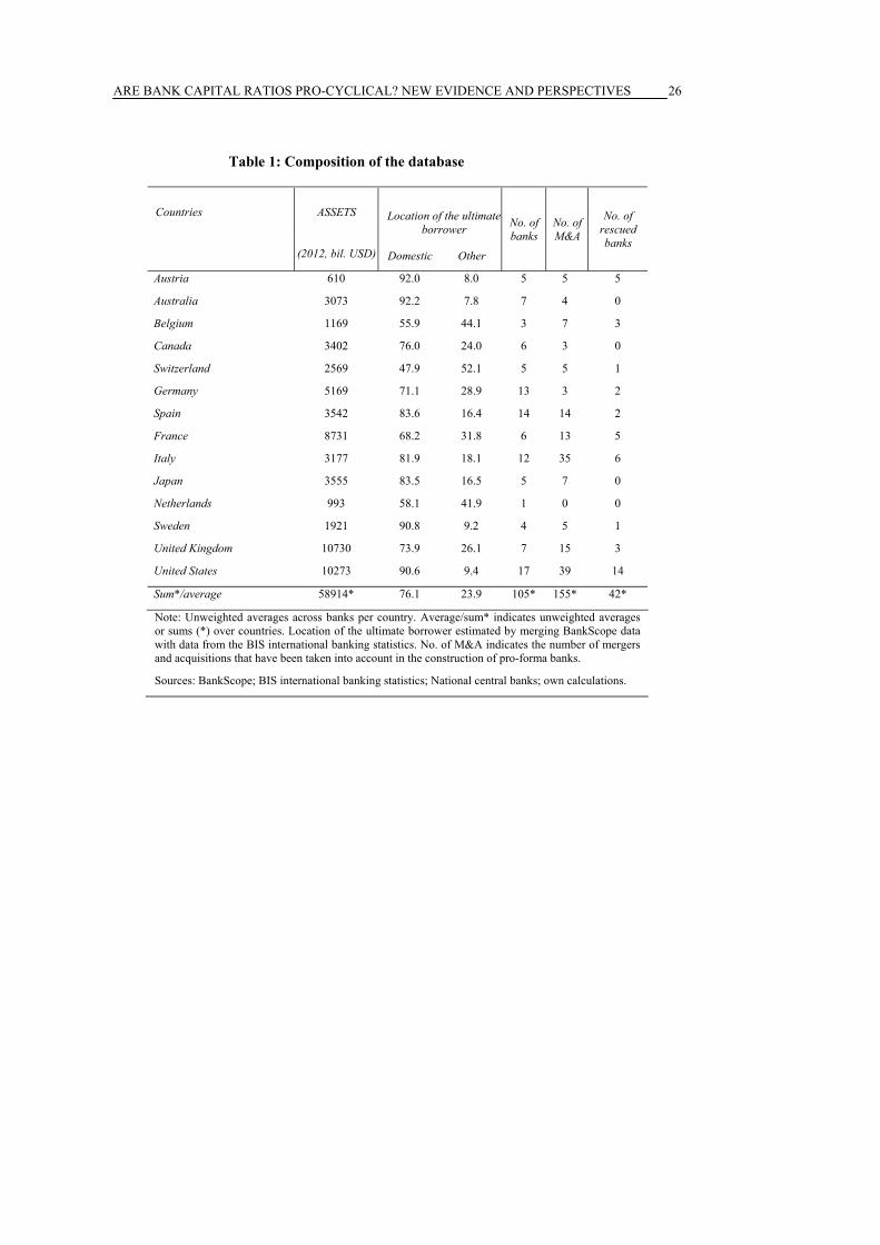
ARE BANK CAPITAL RATIOS PRO-CYCLICAL? NEW EVIDENCE AND PERSPECTIVES
26
Table 1: Composition of the database
Countries ASSETS Location of the ultimate borrower No. of
banks No. of M&A
No. of rescued banks
(2012, bil. USD) Domestic Other
Austria 610 92.0 8.0 5 5 5
Australia 3073 92.2 7.8 7 4 0
Belgium 1169 55.9 44.1 3 7 3
Canada 3402 76.0 24.0 6 3 0
Switzerland 2569 47.9 52.1 5 5 1
Germany 5169 71.1 28.9 13 3 2
Spain 3542 83.6 16.4 14 14 2
France 8731 68.2 31.8 6 13 5
Italy 3177 81.9 18.1 12 35 6
Japan 3555 83.5 16.5 5 7 0
Netherlands 993 58.1 41.9 1 0 0
Sweden 1921 90.8 9.2 4 5 1
United Kingdom 10730 73.9 26.1 7 15 3
United States 10273 90.6 9.4 17 39 14
Sum*/average 58914* 76.1 23.9 105* 155* 42*
Note: Unweighted averages across banks per country. Average/sum* indicates unweighted averages or sums (*) over countries. Location of the ultimate borrower estimated by merging BankScope data with data from the BIS international banking statistics. No. of M&A indicates the number of mergers and acquisitions that have been taken into account in the construction of pro-forma banks.
Sources: BankScope; BIS international banking statistics; National central banks; own calculations.
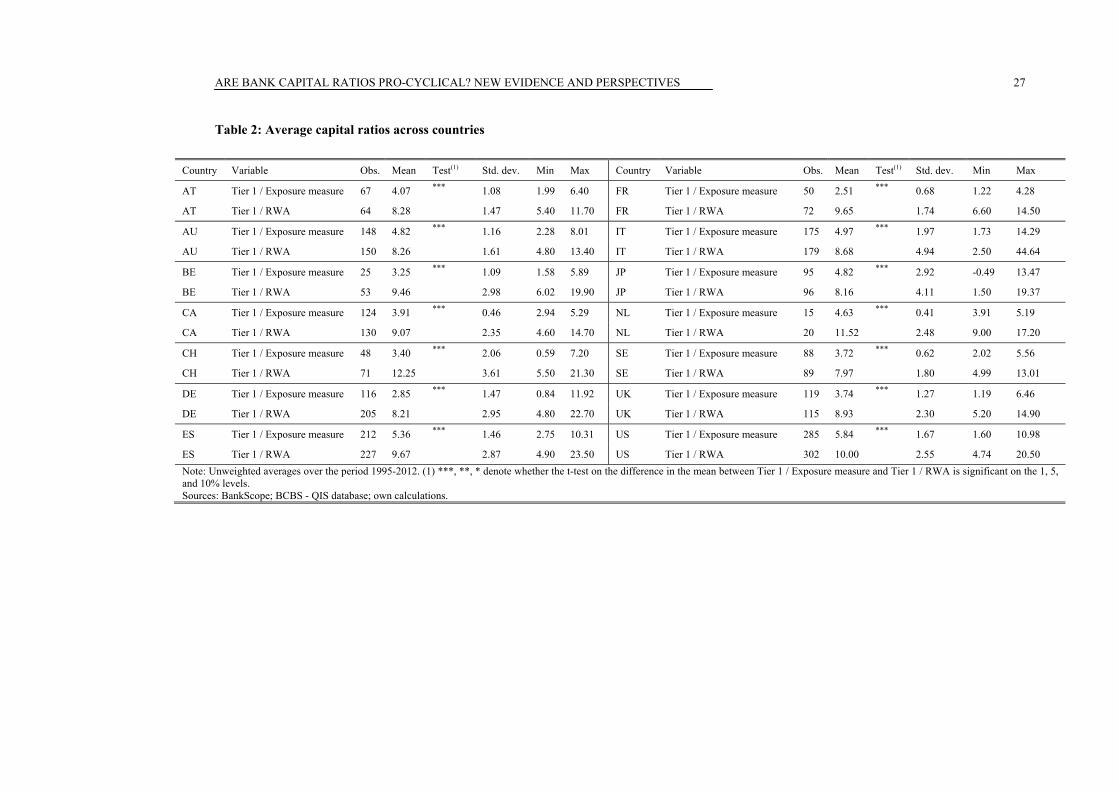
ARE BANK CAPITAL RATIOS PRO-CYCLICAL? NEW EVIDENCE AND PERSPECTIVES
27
Table 2: Average capital ratios across countries
Country Variable Obs. Mean Test(1) Std. dev. Min Max Country Variable Obs. Mean Test(1) Std. dev. Min Max
AT Tier 1 / Exposure measure 67 4.07 *** 1.08 1.99 6.40 FR Tier 1 / Exposure measure 50 2.51 *** 0.68 1.22 4.28
AT Tier 1 / RWA 64 8.28 1.47 5.40 11.70 FR Tier 1 / RWA 72 9.65 1.74 6.60 14.50
AU Tier 1 / Exposure measure 148 4.82 *** 1.16 2.28 8.01 IT Tier 1 / Exposure measure 175 4.97 *** 1.97 1.73 14.29
AU Tier 1 / RWA 150 8.26 1.61 4.80 13.40 IT Tier 1 / RWA 179 8.68 4.94 2.50 44.64
BE Tier 1 / Exposure measure 25 3.25 *** 1.09 1.58 5.89 JP Tier 1 / Exposure measure 95 4.82 *** 2.92 -0.49 13.47
BE Tier 1 / RWA 53 9.46 2.98 6.02 19.90 JP Tier 1 / RWA 96 8.16 4.11 1.50 19.37
CA Tier 1 / Exposure measure 124 3.91 *** 0.46 2.94 5.29 NL Tier 1 / Exposure measure 15 4.63 *** 0.41 3.91 5.19
CA Tier 1 / RWA 130 9.07 2.35 4.60 14.70 NL Tier 1 / RWA 20 11.52 2.48 9.00 17.20
CH Tier 1 / Exposure measure 48 3.40 *** 2.06 0.59 7.20 SE Tier 1 / Exposure measure 88 3.72 *** 0.62 2.02 5.56
CH Tier 1 / RWA 71 12.25 3.61 5.50 21.30 SE Tier 1 / RWA 89 7.97 1.80 4.99 13.01
DE Tier 1 / Exposure measure 116 2.85 *** 1.47 0.84 11.92 UK Tier 1 / Exposure measure 119 3.74 *** 1.27 1.19 6.46
DE Tier 1 / RWA 205 8.21 2.95 4.80 22.70 UK Tier 1 / RWA 115 8.93 2.30 5.20 14.90
ES Tier 1 / Exposure measure 212 5.36 *** 1.46 2.75 10.31 US Tier 1 / Exposure measure 285 5.84 *** 1.67 1.60 10.98
ES Tier 1 / RWA 227 9.67 2.87 4.90 23.50 US Tier 1 / RWA 302 10.00 2.55 4.74 20.50 Note: Unweighted averages over the period 1995-2012. (1) ***, **, * denote whether the t-test on the difference in the mean between Tier 1 / Exposure measure and Tier 1 / RWA is significant on the 1, 5, and 10% levels. Sources: BankScope; BCBS - QIS database; own calculations.
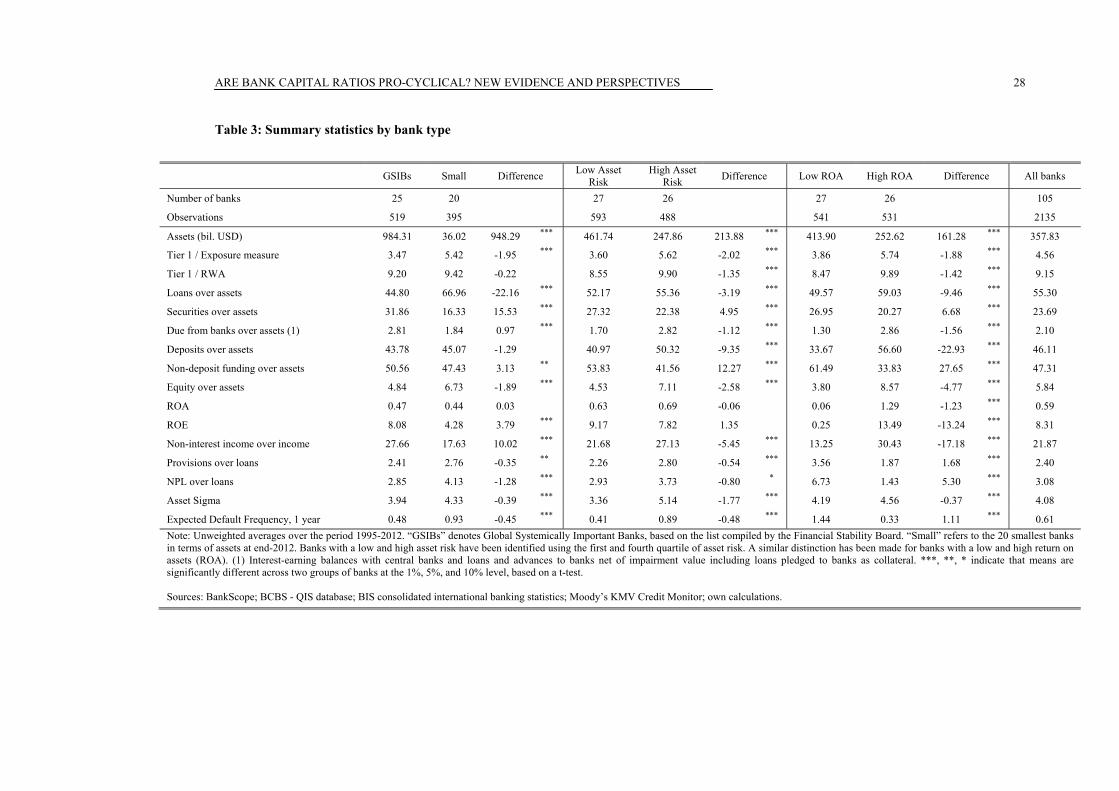
ARE BANK CAPITAL RATIOS PRO-CYCLICAL? NEW EVIDENCE AND PERSPECTIVES
28
Table 3: Summary statistics by bank type
GSIBs Small Difference Low Asset Risk
High Asset Risk Difference Low ROA High ROA Difference All banks
Number of banks 25 20 27 26 27 26 105
Observations 519 395 593 488 541 531 2135
Assets (bil. USD) 984.31 36.02 948.29 *** 461.74 247.86 213.88 *** 413.90 252.62 161.28 *** 357.83
Tier 1 / Exposure measure 3.47 5.42 -1.95 *** 3.60 5.62 -2.02 *** 3.86 5.74 -1.88 *** 4.56
Tier 1 / RWA 9.20 9.42 -0.22 8.55 9.90 -1.35 *** 8.47 9.89 -1.42 *** 9.15
Loans over assets 44.80 66.96 -22.16 *** 52.17 55.36 -3.19 *** 49.57 59.03 -9.46 *** 55.30
Securities over assets 31.86 16.33 15.53 *** 27.32 22.38 4.95 *** 26.95 20.27 6.68 *** 23.69
Due from banks over assets (1) 2.81 1.84 0.97 *** 1.70 2.82 -1.12 *** 1.30 2.86 -1.56 *** 2.10
Deposits over assets 43.78 45.07 -1.29 40.97 50.32 -9.35 *** 33.67 56.60 -22.93 *** 46.11
Non-deposit funding over assets 50.56 47.43 3.13 ** 53.83 41.56 12.27 *** 61.49 33.83 27.65 *** 47.31
Equity over assets 4.84 6.73 -1.89 *** 4.53 7.11 -2.58 *** 3.80 8.57 -4.77 *** 5.84
ROA 0.47 0.44 0.03 0.63 0.69 -0.06 0.06 1.29 -1.23 *** 0.59
ROE 8.08 4.28 3.79 *** 9.17 7.82 1.35 0.25 13.49 -13.24 *** 8.31
Non-interest income over income 27.66 17.63 10.02 *** 21.68 27.13 -5.45 *** 13.25 30.43 -17.18 *** 21.87
Provisions over loans 2.41 2.76 -0.35 ** 2.26 2.80 -0.54 *** 3.56 1.87 1.68 *** 2.40
NPL over loans 2.85 4.13 -1.28 *** 2.93 3.73 -0.80 * 6.73 1.43 5.30 *** 3.08
Asset Sigma 3.94 4.33 -0.39 *** 3.36 5.14 -1.77 *** 4.19 4.56 -0.37 *** 4.08
Expected Default Frequency, 1 year 0.48 0.93 -0.45 *** 0.41 0.89 -0.48 *** 1.44 0.33 1.11 *** 0.61 Note: Unweighted averages over the period 1995-2012. “GSIBs” denotes Global Systemically Important Banks, based on the list compiled by the Financial Stability Board. “Small” refers to the 20 smallest banks in terms of assets at end-2012. Banks with a low and high asset risk have been identified using the first and fourth quartile of asset risk. A similar distinction has been made for banks with a low and high return on assets (ROA). (1) Interest-earning balances with central banks and loans and advances to banks net of impairment value including loans pledged to banks as collateral. ***, **, * indicate that means are significantly different across two groups of banks at the 1%, 5%, and 10% level, based on a t-test. Sources: BankScope; BCBS - QIS database; BIS consolidated international banking statistics; Moody’s KMV Credit Monitor; own calculations.
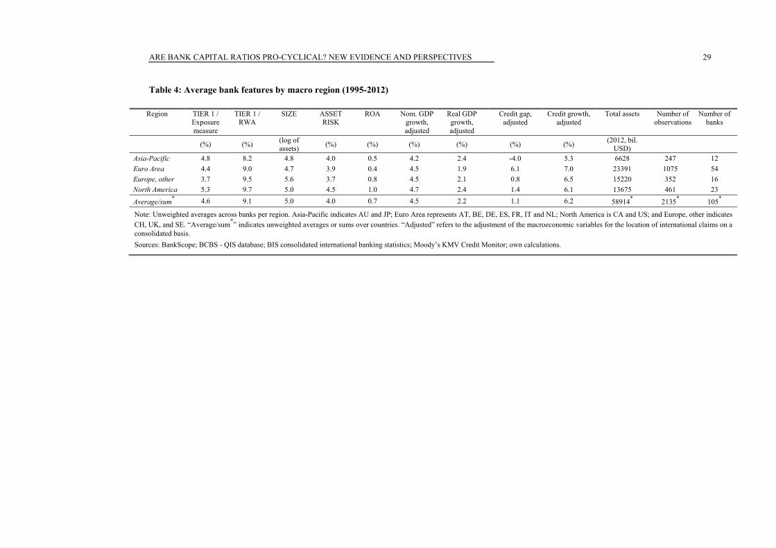
ARE BANK CAPITAL RATIOS PRO-CYCLICAL? NEW EVIDENCE AND PERSPECTIVES
29
Table 4: Average bank features by macro region (1995-2012)
Region TIER 1 / Exposure measure
TIER 1 / RWA
SIZE ASSET RISK
ROA Nom. GDP growth, adjusted
Real GDP growth, adjusted
Credit gap, adjusted
Credit growth, adjusted
Total assets Number of observations
Number of banks
(%) (%) (log of assets) (%) (%) (%) (%) (%) (%) (2012, bil.
USD)
Asia-Pacific 4.8 8.2 4.8 4.0 0.5 4.2 2.4 -4.0 5.3 6628 247 12 Euro Area 4.4 9.0 4.7 3.9 0.4 4.5 1.9 6.1 7.0 23391 1075 54 Europe, other 3.7 9.5 5.6 3.7 0.8 4.5 2.1 0.8 6.5 15220 352 16 North America 5.3 9.7 5.0 4.5 1.0 4.7 2.4 1.4 6.1 13675 461 23 Average/sum* 4.6 9.1 5.0 4.0 0.7 4.5 2.2 1.1 6.2 58914* 2135* 105*
Note: Unweighted averages across banks per region. Asia-Pacific indicates AU and JP; Euro Area represents AT, BE, DE, ES, FR, IT and NL; North America is CA and US; and Europe, other indicates CH, UK, and SE. “Average/sum*” indicates unweighted averages or sums over countries. “Adjusted” refers to the adjustment of the macroeconomic variables for the location of international claims on a consolidated basis. Sources: BankScope; BCBS - QIS database; BIS consolidated international banking statistics; Moody’s KMV Credit Monitor; own calculations.
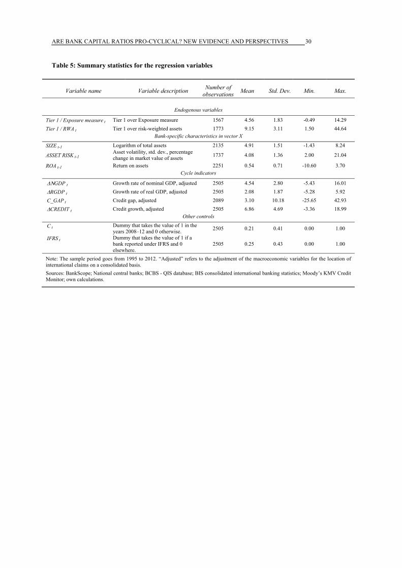
ARE BANK CAPITAL RATIOS PRO-CYCLICAL? NEW EVIDENCE AND PERSPECTIVES
30
Table 5: Summary statistics for the regression variables
Variable name Variable description Number of observations Mean Std. Dev. Min. Max.
Endogenous variables
Tier 1 / Exposure measure t Tier 1 over Exposure measure 1567 4.56 1.83 -0.49 14.29 Tier 1 / RWA t Tier 1 over risk-weighted assets 1773 9.15 3.11 1.50 44.64
Bank-specific characteristics in vector X
SIZE t-1 Logarithm of total assets 2135 4.91 1.51 -1.43 8.24
ASSET RISK t-1 Asset volatility, std. dev., percentage change in market value of assets 1737 4.08 1.36 2.00 21.04
ROA t-1 Return on assets 2251 0.54 0.71 -10.60 3.70 Cycle indicators
GDP t Growth rate of nominal GDP, adjusted 2505 4.54 2.80 -5.43 16.01 RGDP t Growth rate of real GDP, adjusted 2505 2.08 1.87 -5.28 5.92 C_GAP t Credit gap, adjusted 2089 3.10 10.18 -25.65 42.93 CREDIT t Credit growth, adjusted 2505 6.86 4.69 -3.36 18.99
Other controls
C t Dummy that takes the value of 1 in the years 2008–12 and 0 otherwise. 2505 0.21 0.41 0.00 1.00
IFRS t
Dummy that takes the value of 1 if a bank reported under IFRS and 0 elsewhere.
2505 0.25 0.43 0.00 1.00
Note: The sample period goes from 1995 to 2012. “Adjusted” refers to the adjustment of the macroeconomic variables for the location of international claims on a consolidated basis. Sources: BankScope; National central banks; BCBS - QIS database; BIS consolidated international banking statistics; Moody’s KMV Credit Monitor; own calculations.
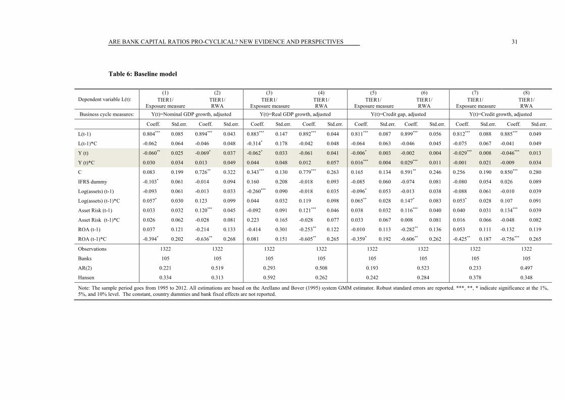
ARE BANK CAPITAL RATIOS PRO-CYCLICAL? NEW EVIDENCE AND PERSPECTIVES
31
Table 6: Baseline model
Dependent variable L(t): (1) (2) (3) (4) (5) (6) (7) (8)
TIER1/ Exposure measure
TIER1/ RWA
TIER1/ Exposure measure
TIER1/ RWA
TIER1/ Exposure measure
TIER1/ RWA
TIER1/ Exposure measure
TIER1/ RWA
Business cycle measures: Y(t)=Nominal GDP growth, adjusted Y(t)=Real GDP growth, adjusted Y(t)=Credit gap, adjusted Y(t)=Credit growth, adjusted
Coeff. Std.err. Coeff. Std.err. Coeff. Std.err. Coeff. Std.err. Coeff. Std.err. Coeff. Std.err. Coeff. Std.err. Coeff. Std.err.
L(t-1) 0.804*** 0.085 0.894*** 0.043 0.883*** 0.147 0.892*** 0.044 0.811*** 0.087 0.899*** 0.056 0.812*** 0.088 0.885*** 0.049
L(t-1)*C -0.062 0.064 -0.046 0.048 -0.314* 0.178 -0.042 0.048 -0.064 0.063 -0.046 0.045 -0.075 0.067 -0.041 0.049
Y (t) -0.060** 0.025 -0.069* 0.037 -0.062* 0.033 -0.061 0.041 -0.006* 0.003 -0.002 0.004 -0.029*** 0.008 -0.046*** 0.013
Y (t)*C 0.030 0.034 0.013 0.049 0.044 0.048 0.012 0.057 0.016*** 0.004 0.029*** 0.011 -0.001 0.021 -0.009 0.034
C 0.083 0.199 0.726** 0.322 0.343*** 0.130 0.779*** 0.263 0.165 0.134 0.591** 0.246 0.256 0.190 0.850*** 0.280
IFRS dummy -0.103* 0.061 -0.014 0.094 0.160 0.208 -0.018 0.093 -0.085 0.060 -0.074 0.081 -0.080 0.054 0.026 0.089
Log(assets) (t-1) -0.093 0.061 -0.013 0.033 -0.260*** 0.090 -0.018 0.035 -0.096* 0.053 -0.013 0.038 -0.088 0.061 -0.010 0.039
Log(assets) (t-1)*C 0.057* 0.030 0.123 0.099 0.044 0.032 0.119 0.098 0.065** 0.028 0.147* 0.083 0.053* 0.028 0.107 0.091
Asset Risk (t-1) 0.033 0.032 0.120*** 0.045 -0.092 0.091 0.121*** 0.046 0.038 0.032 0.116*** 0.040 0.040 0.031 0.134*** 0.039
Asset Risk (t-1)*C 0.026 0.062 -0.028 0.081 0.223 0.165 -0.028 0.077 0.033 0.067 0.008 0.081 0.016 0.066 -0.048 0.082
ROA (t-1) 0.037 0.121 -0.214 0.133 -0.414 0.301 -0.253** 0.122 -0.010 0.113 -0.282** 0.136 0.053 0.111 -0.132 0.119
ROA (t-1)*C -0.394* 0.202 -0.636** 0.268 0.081 0.151 -0.605** 0.265 -0.359* 0.192 -0.606** 0.262 -0.425** 0.187 -0.756*** 0.265
Observations 1322 1322 1322 1322 1322 1322 1322 1322
Banks 105 105 105 105 105 105 105 105
AR(2) 0.221 0.519 0.293 0.508 0.193 0.523 0.233 0.497
Hansen 0.334 0.313 0.592 0.262 0.242 0.284 0.378 0.348
Note: The sample period goes from 1995 to 2012. All estimations are based on the Arellano and Bover (1995) system GMM estimator. Robust standard errors are reported. ***, **, * indicate significance at the 1%, 5%, and 10% level. The constant, country dummies and bank fixed effects are not reported.
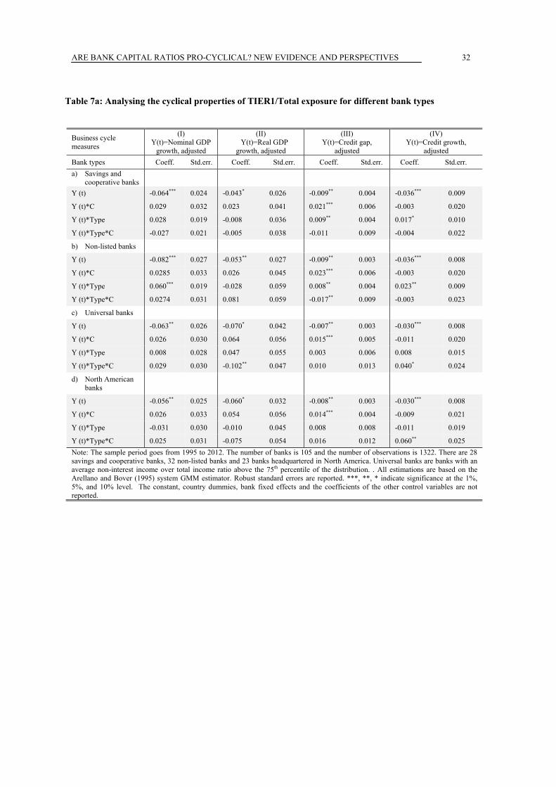
ARE BANK CAPITAL RATIOS PRO-CYCLICAL? NEW EVIDENCE AND PERSPECTIVES
32
Table 7a: Analysing the cyclical properties of TIER1/Total exposure for different bank types
Business cycle measures
(I) (II) Y(t)=Real GDP
growth, adjusted
(III) (IV) Y(t)=Nominal GDP
growth, adjusted Y(t)=Credit gap,
adjusted Y(t)=Credit growth,
adjusted Bank types Coeff. Std.err. Coeff. Std.err. Coeff. Std.err. Coeff. Std.err. a) Savings and
cooperative banks
Y (t) -0.064*** 0.024 -0.043* 0.026 -0.009** 0.004 -0.036*** 0.009
Y (t)*C 0.029 0.032 0.023 0.041 0.021*** 0.006 -0.003 0.020
Y (t)*Type 0.028 0.019 -0.008 0.036 0.009** 0.004 0.017* 0.010
Y (t)*Type*C -0.027 0.021 -0.005 0.038 -0.011 0.009 -0.004 0.022
b) Non-listed banks
Y (t) -0.082*** 0.027 -0.053** 0.027 -0.009** 0.003 -0.036*** 0.008
Y (t)*C 0.0285 0.033 0.026 0.045 0.023*** 0.006 -0.003 0.020
Y (t)*Type 0.060*** 0.019 -0.028 0.059 0.008** 0.004 0.023** 0.009
Y (t)*Type*C 0.0274 0.031 0.081 0.059 -0.017** 0.009 -0.003 0.023
c) Universal banks
Y (t) -0.063** 0.026 -0.070* 0.042 -0.007** 0.003 -0.030*** 0.008
Y (t)*C 0.026 0.030 0.064 0.056 0.015*** 0.005 -0.011 0.020
Y (t)*Type 0.008 0.028 0.047 0.055 0.003 0.006 0.008 0.015
Y (t)*Type*C 0.029 0.030 -0.102** 0.047 0.010 0.013 0.040* 0.024
d) North American banks
Y (t) -0.056** 0.025 -0.060* 0.032 -0.008** 0.003 -0.030*** 0.008
Y (t)*C 0.026 0.033 0.054 0.056 0.014*** 0.004 -0.009 0.021
Y (t)*Type -0.031 0.030 -0.010 0.045 0.008 0.008 -0.011 0.019
Y (t)*Type*C 0.025 0.031 -0.075 0.054 0.016 0.012 0.060** 0.025 Note: The sample period goes from 1995 to 2012. The number of banks is 105 and the number of observations is 1322. There are 28 savings and cooperative banks, 32 non-listed banks and 23 banks headquartered in North America. Universal banks are banks with an average non-interest income over total income ratio above the 75th percentile of the distribution. . All estimations are based on the Arellano and Bover (1995) system GMM estimator. Robust standard errors are reported. ***, **, * indicate significance at the 1%, 5%, and 10% level. The constant, country dummies, bank fixed effects and the coefficients of the other control variables are not reported.
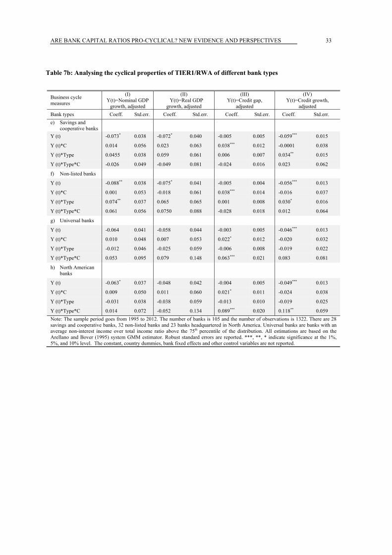
ARE BANK CAPITAL RATIOS PRO-CYCLICAL? NEW EVIDENCE AND PERSPECTIVES
33
Table 7b: Analysing the cyclical properties of TIER1/RWA of different bank types
Business cycle measures
(I) (II) Y(t)=Real GDP
growth, adjusted
(III) (IV) Y(t)=Nominal GDP
growth, adjusted Y(t)=Credit gap,
adjusted Y(t)=Credit growth,
adjusted Bank types Coeff. Std.err. Coeff. Std.err. Coeff. Std.err. Coeff. Std.err. e) Savings and
cooperative banks
Y (t) -0.073* 0.038 -0.072* 0.040 -0.005 0.005 -0.059*** 0.015
Y (t)*C 0.014 0.056 0.023 0.063 0.038*** 0.012 -0.0001 0.038
Y (t)*Type 0.0455 0.038 0.059 0.061 0.006 0.007 0.034** 0.015
Y (t)*Type*C -0.026 0.049 -0.049 0.081 -0.024 0.016 0.023 0.062
f) Non-listed banks
Y (t) -0.088** 0.038 -0.075* 0.041 -0.005 0.004 -0.056*** 0.013
Y (t)*C 0.001 0.053 -0.018 0.061 0.038*** 0.014 -0.016 0.037
Y (t)*Type 0.074** 0.037 0.065 0.065 0.001 0.008 0.030* 0.016
Y (t)*Type*C 0.061 0.056 0.0750 0.088 -0.028 0.018 0.012 0.064
g) Universal banks
Y (t) -0.064 0.041 -0.058 0.044 -0.003 0.005 -0.046*** 0.013
Y (t)*C 0.010 0.048 0.007 0.053 0.022* 0.012 -0.020 0.032
Y (t)*Type -0.012 0.046 -0.025 0.059 -0.006 0.008 -0.019 0.022
Y (t)*Type*C 0.053 0.095 0.079 0.148 0.063*** 0.021 0.083 0.081
h) North American banks
Y (t) -0.063* 0.037 -0.048 0.042 -0.004 0.005 -0.049*** 0.013
Y (t)*C 0.009 0.050 0.011 0.060 0.021* 0.011 -0.024 0.038
Y (t)*Type -0.031 0.038 -0.038 0.059 -0.013 0.010 -0.019 0.025
Y (t)*Type*C 0.014 0.072 -0.052 0.134 0.089*** 0.020 0.118** 0.059 Note: The sample period goes from 1995 to 2012. The number of banks is 105 and the number of observations is 1322. There are 28 savings and cooperative banks, 32 non-listed banks and 23 banks headquartered in North America. Universal banks are banks with an average non-interest income over total income ratio above the 75th percentile of the distribution. All estimations are based on the Arellano and Bover (1995) system GMM estimator. Robust standard errors are reported. ***, **, * indicate significance at the 1%, 5%, and 10% level. The constant, country dummies, bank fixed effects and other control variables are not reported.

ARE BANK CAPITAL RATIOS PRO-CYCLICAL? NEW EVIDENCE AND PERSPECTIVES
34
Table 8: Controlling for different regimes in capital regulation
Dependent variable L(t): (25) (26) (27) (28) (29) (30) (31) (32)
TIER1/ Total Exposure
TIER1/ RWA
TIER1/ Total Exposure
TIER1/ RWA
TIER1/ Total Exposure
TIER1/ RWA
TIER1/ Total Exposure
TIER1/ RWA
Business cycle measures: Y(t)=Nominal GDP growth, adjusted Y(t)=Real GDP growth, adjusted Y(t)=Credit gap, adjusted Y(t)=Credit growth, adjusted
Coeff. Std.err. Coeff. Std.err. Coeff. Std.err. Coeff. Std.err. Coeff. Std.err. Coeff. Std.err. Coeff. Std.err. Coeff. Std.err.
L(t-1) 0.776*** 0.087 0.884*** 0.046 0.774*** 0.091 0.880*** 0.044 0.781*** 0.078 0.892*** 0.057 0.788*** 0.083 0.879*** 0.052
L(t-1)*C -0.058 0.063 -0.036 0.047 -0.058 0.062 -0.034 0.050 -0.059 0.062 -0.038 0.046 -0.052 0.062 -0.033 0.048
Y (t) -0.065** 0.025 -0.066* 0.035 -0.050* 0.025 -0.059 0.042 -0.007** 0.003 -0.002 0.004 -0.029*** 0.009 -0.017 0.014
Y (t)*C 0.032 0.035 0.006 0.054 -0.005 0.041 -0.064 0.079 0.014*** 0.004 0.031** 0.013 -0.016 0.022 -0.013 0.036
Basel II -0.259 0.214 -0.414*** 0.152 -0.274* 0.152 -0.284 0.268
Y(t)*Basel II 0.004 0.047 0.077 0.063 -0.002 0.009 0.010 0.028
Leverage regulation 0.492 0.313 0.584* 0.330 0.447** 0.182 0.393 0.263
Y(t)*Leverage regulation -0.024 0.028 -0.046 0.045 0.006 0.008 -0.013 0.017
Y(t)*Leverage regulation*C 0.026 0.027 0.003 0.049 0.017 0.012 0.061 0.055
C 0.037 0.202 0.926*** 0.309 0.231* 0.136 1.088*** 0.262 0.133 0.128 0.735*** 0.260 0.267 0.193 1.030*** 0.299
IFRS dummy -0.032 0.063 0.047 0.085 -0.043 0.064 0.050 0.089 -0.038 0.066 0.008 0.079 -0.011 0.066 0.084 0.085
Log(assets) (t-1) -0.136** 0.066 -0.011 0.038 -0.135* 0.072 -0.021 0.039 -0.120** 0.054 -0.012 0.040 -0.117** 0.055 -0.011 0.045
Log(assets) (t-1)*C 0.058* 0.032 0.120 0.104 0.060* 0.036 0.130 0.104 0.052* 0.028 0.152* 0.086 0.050* 0.029 0.110 0.099
Bank risk (t-1) 0.047 0.033 0.128*** 0.046 0.056* 0.033 0.135*** 0.050 0.053* 0.032 0.120*** 0.040 0.063** 0.029 0.138*** 0.039
Bank risk (t-1)*C 0.015 0.070 -0.037 0.089 0.012 0.072 -0.038 0.079 0.049 0.073 0.005 0.084 -0.018 0.059 -0.057 0.097
ROA (t-1) 0.057 0.134 -0.131 0.145 0.008 0.120 -0.142 0.133 -0.014 0.121 -0.207 0.143 0.084 0.135 -0.050 0.139
ROA (t-1)*C -0.416* 0.216 -0.717*** 0.259 -0.349* 0.198 -0.702*** 0.266 -0.343* 0.183 -0.676** 0.269 -0.443** 0.196 -0.844*** 0.279
Observations 1322 1322 1322 1322 1322 1322 1322 1322
Banks 105 105 105 105 105 105 105 105
AR(2) 0.148 0.522 0.115 0.535 0.119 0.532 0.172 0.502
Hansen 0.361 0.318 0.365 0.272 0.295 0.284 0.446 0.322 Note: The sample period goes from 1995 to 2012. All estimations are based on the Arellano and Bover (1995) system GMM estimator. Robust standard errors are reported. ***, **, * indicate significance at the 1%, 5%, and 10% level. The constant, country dummies and bank fixed effects are not reported.
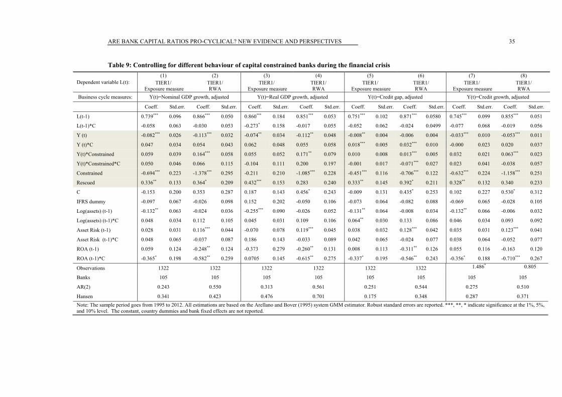
ARE BANK CAPITAL RATIOS PRO-CYCLICAL? NEW EVIDENCE AND PERSPECTIVES
35
Table 9: Controlling for different behaviour of capital constrained banks during the financial crisis
Dependent variable L(t): (1) (2) (3) (4) (5) (6) (7) (8)
TIER1/ Exposure measure
TIER1/ RWA
TIER1/ Exposure measure
TIER1/ RWA
TIER1/ Exposure measure
TIER1/ RWA
TIER1/ Exposure measure
TIER1/ RWA
Business cycle measures: Y(t)=Nominal GDP growth, adjusted Y(t)=Real GDP growth, adjusted Y(t)=Credit gap, adjusted Y(t)=Credit growth, adjusted
Coeff. Std.err. Coeff. Std.err. Coeff. Std.err. Coeff. Std.err. Coeff. Std.err. Coeff. Std.err. Coeff. Std.err. Coeff. Std.err.
L(t-1) 0.739*** 0.096 0.866*** 0.050 0.860*** 0.184 0.851*** 0.053 0.751*** 0.102 0.871*** 0.0580 0.745*** 0.099 0.855*** 0.051
L(t-1)*C -0.058 0.063 -0.030 0.053 -0.273* 0.158 -0.017 0.055 -0.052 0.062 -0.024 0.0499 -0.077 0.068 -0.019 0.056
Y (t) -0.082*** 0.026 -0.113*** 0.032 -0.074** 0.034 -0.112** 0.048 -0.008** 0.004 -0.006 0.004 -0.033*** 0.010 -0.053*** 0.011
Y (t)*C 0.047 0.034 0.054 0.043 0.062 0.048 0.055 0.058 0.018*** 0.005 0.032*** 0.010 -0.000 0.023 0.020 0.037
Y(t)*Constrained 0.059 0.039 0.164*** 0.058 0.055 0.052 0.171** 0.079 0.010 0.008 0.013*** 0.005 0.032 0.021 0.063*** 0.023
Y(t)*Constrained*C 0.050 0.046 0.066 0.115 -0.104 0.111 0.200 0.197 -0.001 0.017 -0.071*** 0.027 0.023 0.041 -0.038 0.057
Constrained -0.694*** 0.223 -1.378*** 0.295 -0.211 0.210 -1.085*** 0.228 -0.451*** 0.116 -0.706*** 0.122 -0.632*** 0.224 -1.158*** 0.251
Rescued 0.336** 0.133 0.364* 0.209 0.432*** 0.153 0.283 0.240 0.333** 0.145 0.392* 0.211 0.328** 0.132 0.340 0.233
C -0.153 0.200 0.353 0.287 0.187 0.143 0.456* 0.243 -0.009 0.131 0.435* 0.253 0.102 0.227 0.530* 0.312
IFRS dummy -0.097 0.067 -0.026 0.098 0.152 0.202 -0.050 0.106 -0.073 0.064 -0.082 0.088 -0.069 0.065 -0.028 0.105
Log(assets) (t-1) -0.132** 0.063 -0.024 0.036 -0.255*** 0.090 -0.026 0.052 -0.131** 0.064 -0.008 0.034 -0.132** 0.066 -0.006 0.032
Log(assets) (t-1)*C 0.048 0.034 0.112 0.105 0.045 0.031 0.109 0.106 0.064** 0.030 0.133 0.086 0.046 0.034 0.093 0.092
Asset Risk (t-1) 0.028 0.031 0.116*** 0.044 -0.070 0.078 0.119*** 0.045 0.038 0.032 0.128*** 0.042 0.035 0.031 0.123*** 0.041
Asset Risk (t-1)*C 0.048 0.065 -0.037 0.087 0.186 0.143 -0.033 0.089 0.042 0.065 -0.024 0.077 0.038 0.064 -0.052 0.077
ROA (t-1) 0.059 0.124 -0.248** 0.124 -0.373 0.279 -0.260** 0.131 0.008 0.113 -0.311** 0.126 0.055 0.116 -0.163 0.120
ROA (t-1)*C -0.365* 0.198 -0.582** 0.259 0.0705 0.145 -0.615** 0.275 -0.337* 0.195 -0.546** 0.243 -0.356* 0.188 -0.710*** 0.267
Observations 1322 1322 1322 1322 1322 1322 1.486* 0.805
Banks 105 105 105 105 105 105 105 105
AR(2) 0.243 0.550 0.313 0.561 0.251 0.544 0.275 0.510
Hansen 0.341 0.423 0.476 0.701 0.175 0.348 0.287 0.371 Note: The sample period goes from 1995 to 2012. All estimations are based on the Arellano and Bover (1995) system GMM estimator. Robust standard errors are reported. ***, **, * indicate significance at the 1%, 5%, and 10% level. The constant, country dummies and bank fixed effects are not reported.
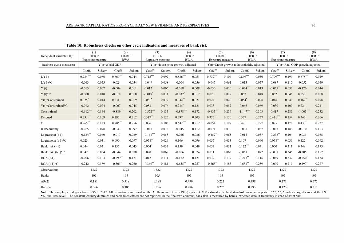
ARE BANK CAPITAL RATIOS PRO-CYCLICAL? NEW EVIDENCE AND PERSPECTIVES
36
Table 10: Robustness checks on other cycle indicators and measures of bank risk
Dependent variable L(t): (1) (2) (3) (4) (5) (6) (7) (8)
TIER1/ Exposure measure
TIER1/ RWA
TIER1/ Exposure measure
TIER1/ RWA
TIER1/ Exposure measure
TIER1/ RWA
TIER1/ Exposure measure
TIER1/ RWA
Business cycle measures: Y(t)=World GDP Y(t)=House price growth, adjusted Y(t)=Credit growth to households, adjusted Y(t)= Real GDP growth, adjusted
Coeff. Std.err. Coeff. Std.err. Coeff. Std.err. Coeff. Std.err. Coeff. Std.err. Coeff. Std.err. Coeff. Std.err. Coeff. Std.err.
L(t-1) 0.734*** 0.086 0.860*** 0.044 0.715*** 0.092 0.836*** 0.051 0.732*** 0.104 0.849*** 0.050 0.709*** 0.190 0.878*** 0.049
L(t-1)*C -0.063 0.055 -0.024 0.054 -0.049 0.058 -0.004 0.056 -0.047 0.061 -0.013 0.057 -0.087 0.115 -0.052 0.049
Y (t) -0.013* 0.007 -0.004 0.011 -0.012* 0.006 -0.018** 0.008 -0.030*** 0.010 -0.034*** 0.013 -0.079** 0.033 -0.120*** 0.044
Y (t)*C -0.008 0.010 -0.018 0.018 -0.019* 0.011 -0.032* 0.017 0.023 0.029 0.057 0.048 0.052 0.046 0.050 0.058
Y(t)*Constrained 0.025* 0.014 0.031 0.019 0.031* 0.017 0.042** 0.021 0.024 0.020 0.054* 0.028 0.046 0.049 0.162** 0.078
Y(t)*Constrained*C -0.012 0.024 -0.007 0.045 0.083 0.076 0.235* 0.121 0.033 0.057 -0.066 0.069 -0.030 0.109 0.224 0.211
Constrained -0.612*** 0.144 -0.889*** 0.202 -0.572*** 0.135 -0.878*** 0.172 -0.633*** 0.239 -1.147*** 0.303 -0.417 0.285 -1.003*** 0.232
Rescued 0.331*** 0.109 0.295 0.212 0.317** 0.125 0.297 0.205 0.323*** 0.120 0.337 0.237 0.411*** 0.154 0.342* 0.206
C 0.265** 0.123 0.906*** 0.256 0.086 0.103 0.642*** 0.217 -0.054 0.199 0.421 0.297 0.025 0.178 0.433* 0.237
IFRS dummy -0.065 0.078 -0.043 0.097 -0.048 0.073 -0.045 0.112 -0.071 0.070 -0.095 0.087 -0.003 0.189 -0.010 0.103
Log(assets) (t-1) -0.134** 0.060 -0.017 0.039 -0.161*** 0.058 -0.026 0.036 -0.152** 0.065 -0.014 0.037 -0.233** 0.104 -0.031 0.038
Log(assets) (t-1)*C 0.023 0.031 0.090 0.097 0.058** 0.029 0.106 0.096 0.055* 0.033 0.107 0.090 0.078** 0.036 0.122 0.092
Bank risk (t-1) 0.044 0.031 0.136*** 0.043 0.064* 0.033 0.159*** 0.049 0.053* 0.031 0.122*** 0.041 0.060 0.311 0.349** 0.173
Bank risk (t-1)*C 0.042 0.064 -0.044 0.078 0.020 0.067 -0.056 0.074 0.011 0.063 -0.051 0.072 -0.031 0.345 -0.205 0.182
ROA (t-1) -0.006 0.103 -0.299** 0.121 0.042 0.114 -0.172 0.121 0.032 0.119 -0.243** 0.116 -0.069 0.332 -0.250* 0.134
ROA (t-1)*C -0.242 0.189 -0.501* 0.260 -0.360** 0.181 -0.655** 0.257 -0.365** 0.183 -0.651** 0.259 -0.009 0.219 -0.497* 0.277
Observations 1322 1322 1322 1322 1322 1322 1322 1322
Banks 105 105 105 105 105 105 105 105
AR(2) 0.181 0.518 0.188 0.490 0.221 0.498 0.171 0.775
Hansen 0.366 0.303 0.296 0.286 0.275 0.293 0.123 0.311 Note: The sample period goes from 1995 to 2012. All estimations are based on the Arellano and Bover (1995) system GMM estimator. Robust standard errors are reported. ***, **, * indicate significance at the 1%, 5%, and 10% level. The constant, country dummies and bank fixed effects are not reported. In the final two columns, bank risk is measured by banks’ expected default frequency instead of asset risk.
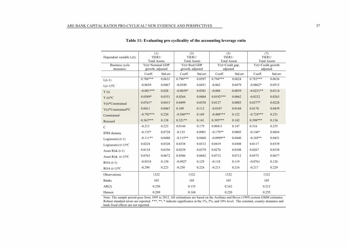
ARE BANK CAPITAL RATIOS PRO-CYCLICAL? NEW EVIDENCE AND PERSPECTIVES
37
Table 11: Evaluating pro cyclicality of the accounting leverage ratio
Dependent variable L(t): (1) (3) (5) (7)
TIER1/ Total Assets
TIER1/ Total Assets
TIER1/ Total Assets
TIER1/ Total Assets
Business cycle measures:
Y(t)=Nominal GDP growth, adjusted
Y(t)=Real GDP growth, adjusted
Y(t)=Credit gap, adjusted
Y(t)=Credit growth adjusted
Coeff. Std.err. Coeff. Std.err. Coeff. Std.err. Coeff. Std.err.
L(t-1) 0.788*** 0.0631 0.790*** 0.0597 0.794*** 0.0624 0.783*** 0.0636
L(t-1)*C -0.0659 0.0467 -0.0549 0.0451 -0.062 0.0479 -0.0862* 0.0515
Y (t) -0.081*** 0.028 -0.0659* 0.0381 -0.004 0.0039 -0.0231** 0.0114
Y (t)*C 0.0589* 0.0351 0.0264 0.0484 0.0192*** 0.0062 -0.0232 0.0263
Y(t)*Constrained 0.0761* 0.0415 0.0499 0.0538 0.0127 0.0085 0.0377* 0.0228
Y(t)*Constrained*C 0.0411 0.0467 0.109 0.112 -0.0107 0.0168 0.0170 0.0439
Constrained -0.792*** 0.220 -0.560*** 0.169 -0.488*** 0.122 -0.724*** 0.251
Rescued 0.363*** 0.138 0.321** 0.141 0.395*** 0.142 0.398*** 0.136
C -0.213 0.223 0.0144 0.179 0.00411 0.147 0.316 0.255
IFRS dummy -0.135* 0.0728 -0.135 0.0901 -0.179** 0.0805 -0.146* 0.0844
Log(assets) (t-1) -0.111** 0.0480 -0.115** 0.0468 -0.0999** 0.0440 -0.105** 0.0431
Log(assets) (t-1)*C 0.0224 0.0328 0.0338 0.0312 0.0419 0.0308 0.0117 0.0339
Asset Risk (t-1) 0.0118 0.0356 0.0239 0.0379 0.0276 0.0348 0.0267 0.0338
Asset Risk (t-1)*C 0.0763 0.0672 0.0506 0.0682 0.0712 0.0712 0.0575 0.0677
ROA (t-1) -0.0518 0.130 -0.0927 0.129 -0.118 0.119 -0.0761 0.126
ROA (t-1)*C -0.290 0.223 -0.250 0.224 -0.213 0.216 -0.217 0.229
Observations 1322 1322 1322 1322
Banks 105 105 105 105
AR(2) 0.250 0.135 0.162 0.212
Hansen 0.209 0.168 0.220 0.255 Note: The sample period goes from 1995 to 2012. All estimations are based on the Arellano and Bover (1995) system GMM estimator. Robust standard errors are reported. ***, **, * indicate significance at the 1%, 5%, and 10% level. The constant, country dummies and bank fixed effects are not reported.
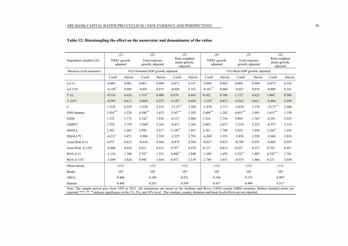
ARE BANK CAPITAL RATIOS PRO-CYCLICAL? NEW EVIDENCE AND PERSPECTIVES
38
Table 12: Disentangling the effect on the numerator and denominator of the ratios
Dependent variable L(t):
(1) (2) (3) (4) (5) (6)
TIER1 growth, adjusted
Total exposure growth, adjusted
Risk-weighted assets growth,
adjusted
TIER1 growth, adjusted
Total exposure growth, adjusted
Risk-weighted assets growth,
adjusted Business cycle measures: Y(t)=Nominal GDP growth, adjusted Y(t)=Real GDP growth, adjusted
Coeff. Std.err. Coeff. Std.err. Coeff. Std.err. Coeff. Std.err. Coeff. Std.err. Coeff. Std.err.
L(t-1) -0.001 0.061 0.063 0.049 -0.071 0.147 -0.004 0.062 0.069 0.049 -0.075 0.143
L(t-1)*C -0.158** 0.069 -0.041 0.075 -0.020 0.163 -0.161** 0.068 -0.027 0.076 -0.009 0.161
Y (t) -0.516 0.626 1.314*** 0.480 0.678 0.443 0.162 0.706 1.175* 0.623 1.004* 0.586
Y (t)*C -0.595 0.613 -0.869 0.555 -0.187 0.436 -1.559* 0.853 -0.562 0.651 -0.406 0.598
C -1.818 4.529 -1.920 3.539 -11.15*** 3.200 -1.470 3.717 -5.034 3.170 -10.72*** 2.606
IFRS dummy 3.954*** 1.220 4.500*** 1.073 3.547*** 1.103 3.808*** 1.202 4.451*** 1.091 3.615*** 1.150
GSIB 1.332 1.771 3.142* 1.836 -0.127 2.000 1.318 1.754 3.098* 1.765 -0.281 2.023
GSIB*C 1.574 2.759 -3.988* 2.165 -0.431 2.365 2.003 2.637 -3.210 2.222 -0.357 2.334
SMALL 2.302 1.685 2.999 2.017 3.149** 1.451 2.261 1.700 3.024 1.896 3.324** 1.436
SMALL*C -6.231* 3.471 -2.900 3.330 -2.325 2.791 -6.200* 3.351 -3.830 2.928 -2.660 2.818
Asset Risk (t-1) 0.075 0.832 -0.610 0.568 -0.876 0.594 -0.017 0.813 -0.789 0.591 -0.885 0.597
Asset Risk (t-1)*C -0.006 0.826 0.431 0.531 0.797* 0.470 0.137 0.815 0.627 0.517 0.743 0.491
ROA (t-1) -1.134 1.709 2.747* 1.531 4.400** 1.840 -1.489 1.692 3.522** 1.403 4.742*** 1.761
ROA (t-1)*C -3.699 3.828 0.948 1.644 0.472 2.139 -2.765 3.631 -0.574 1.466 0.121 2.029
Observations 1151 1151 1151 1151 1151 1151
Banks 105 105 105 105 105 105
AR(2) 0.406 0.100 0.921 0.348 0.151 0.907
Hansen 0.498 0.283 0.549 0.457 0.499 0.517 Note: The sample period goes from 1995 to 2012. All estimations are based on the Arellano and Bover (1995) system GMM estimator. Robust standard errors are reported. ***, **, * indicate significance at the 1%, 5%, and 10% level. The constant, country dummies and bank fixed effects are not reported.
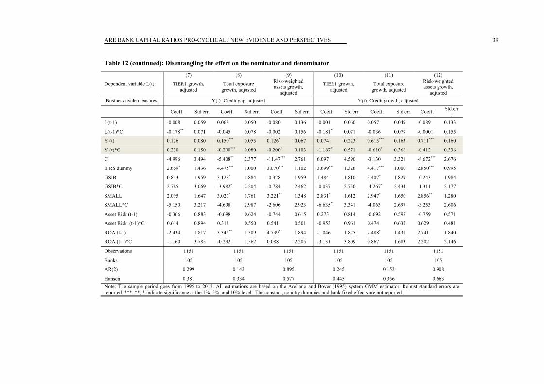
ARE BANK CAPITAL RATIOS PRO-CYCLICAL? NEW EVIDENCE AND PERSPECTIVES
39
Table 12 (continued): Disentangling the effect on the nominator and denominator
Dependent variable L(t):
(7) (8) (9) (10) (11) (12)
TIER1 growth, adjusted
Total exposure growth, adjusted
Risk-weighted assets growth,
adjusted
TIER1 growth, adjusted
Total exposure growth, adjusted
Risk-weighted assets growth,
adjusted Business cycle measures: Y(t)=Credit gap, adjusted Y(t)=Credit growth, adjusted
Coeff. Std.err. Coeff. Std.err. Coeff. Std.err. Coeff. Std.err. Coeff. Std.err. Coeff. Std.err.
L(t-1) -0.008 0.059 0.068 0.050 -0.080 0.136 -0.001 0.060 0.057 0.049 -0.089 0.133
L(t-1)*C -0.178** 0.071 -0.045 0.078 -0.002 0.156 -0.181** 0.071 -0.036 0.079 -0.0001 0.155
Y (t) 0.126 0.080 0.150*** 0.055 0.126* 0.067 0.074 0.223 0.615*** 0.163 0.711*** 0.160
Y (t)*C 0.230 0.150 -0.290*** 0.080 -0.200* 0.103 -1.187** 0.571 -0.610* 0.366 -0.412 0.336
C -4.996 3.494 -5.408** 2.377 -11.47*** 2.761 6.097 4.590 -3.130 3.321 -8.672*** 2.676
IFRS dummy 2.669* 1.436 4.475*** 1.000 3.070*** 1.102 3.699*** 1.326 4.417*** 1.000 2.850*** 0.995
GSIB 0.813 1.959 3.128* 1.884 -0.328 1.959 1.484 1.810 3.407* 1.829 -0.243 1.984
GSIB*C 2.785 3.069 -3.982* 2.204 -0.784 2.462 -0.037 2.750 -4.267* 2.434 -1.311 2.177
SMALL 2.095 1.647 3.027* 1.761 3.221** 1.348 2.831* 1.612 2.947* 1.650 2.856** 1.280
SMALL*C -5.150 3.217 -4.698 2.987 -2.606 2.923 -6.635** 3.341 -4.063 2.697 -3.253 2.606
Asset Risk (t-1) -0.366 0.883 -0.698 0.624 -0.744 0.615 0.273 0.814 -0.692 0.597 -0.759 0.571
Asset Risk (t-1)*C 0.614 0.894 0.318 0.550 0.541 0.501 -0.953 0.961 0.474 0.635 0.629 0.481
ROA (t-1) -2.434 1.817 3.345** 1.509 4.739** 1.894 -1.046 1.825 2.488* 1.431 2.741 1.840
ROA (t-1)*C -1.160 3.785 -0.292 1.562 0.088 2.205 -3.131 3.809 0.867 1.683 2.202 2.146
Observations 1151 1151 1151 1151 1151 1151
Banks 105 105 105 105 105 105
AR(2) 0.299 0.143 0.895 0.245 0.153 0.908
Hansen 0.381 0.334 0.577 0.445 0.356 0.663 Note: The sample period goes from 1995 to 2012. All estimations are based on the Arellano and Bover (1995) system GMM estimator. Robust standard errors are reported. ***, **, * indicate significance at the 1%, 5%, and 10% level. The constant, country dummies and bank fixed effects are not reported.
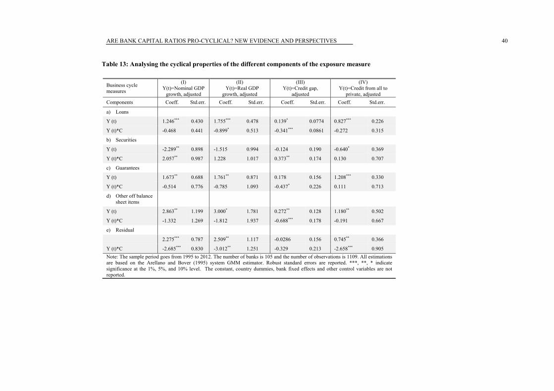
ARE BANK CAPITAL RATIOS PRO-CYCLICAL? NEW EVIDENCE AND PERSPECTIVES
40
Table 13: Analysing the cyclical properties of the different components of the exposure measure
Business cycle measures
(I) (II) Y(t)=Real GDP
growth, adjusted
(III) (IV) Y(t)=Nominal GDP
growth, adjusted Y(t)=Credit gap,
adjusted Y(t)=Credit from all to
private, adjusted Components Coeff. Std.err. Coeff. Std.err. Coeff. Std.err. Coeff. Std.err.
a) Loans
Y (t) 1.246*** 0.430 1.755*** 0.478 0.139* 0.0774 0.827*** 0.226
Y (t)*C -0.468 0.441 -0.899* 0.513 -0.341*** 0.0861 -0.272 0.315
b) Securities
Y (t) -2.289** 0.898 -1.515 0.994 -0.124 0.190 -0.640* 0.369
Y (t)*C 2.057** 0.987 1.228 1.017 0.373** 0.174 0.130 0.707
c) Guarantees
Y (t) 1.673** 0.688 1.761** 0.871 0.178 0.156 1.208*** 0.330
Y (t)*C -0.514 0.776 -0.785 1.093 -0.437* 0.226 0.111 0.713
d) Other off balance sheet items
Y (t) 2.863** 1.199 3.000* 1.781 0.272** 0.128 1.180** 0.502
Y (t)*C -1.332 1.269 -1.812 1.937 -0.688*** 0.178 -0.191 0.667
e) Residual
2.275*** 0.787 2.509** 1.117 -0.0286 0.156 0.745** 0.366
Y (t)*C -2.685*** 0.830 -3.012** 1.251 -0.329 0.213 -2.658*** 0.905 Note: The sample period goes from 1995 to 2012. The number of banks is 105 and the number of observations is 1109. All estimations are based on the Arellano and Bover (1995) system GMM estimator. Robust standard errors are reported. ***, **, * indicate significance at the 1%, 5%, and 10% level. The constant, country dummies, bank fixed effects and other control variables are not reported.

ARE BANK CAPITAL RATIOS PRO-CYCLICAL? NEW EVIDENCE AND PERSPECTIVES
41
Table 14: Evaluating pro cyclicality of a market based measure of the leverage ratio
Dependent variable L(t): (1) (3) (5) (7)
Market equity/ Market assets
Market equity/ Market assets
Market equity/ Market assets
Market equity/ Market assets
Business cycle measures:
Y(t)=Nominal GDP growth, adjusted
Y(t)=Real GDP growth, adjusted
Y(t)=Credit gap, adjusted
Y(t)=Credit from all to private, adjusted
Coeff. Std.err. Coeff. Std.err. Coeff. Std.err. Coeff. Std.err.
L(t-1) 0.605*** 0.112 0.591*** 0.110 0.625*** 0.123 0.607*** 0.120
L(t-1)*C 0.224 0.146 0.227 0.140 0.164 0.137 0.186 0.150
Y (t) 0.130* 0.072 0.301** 0.136 -0.014 0.021 0.022 0.046
Y (t)*C -0.222*** 0.084 -0.378*** 0.139 0.029 0.018 -0.061 0.053
Y(t)*Constrained 0.029 0.127 0.146 0.213 -0.021 0.024 -0.002 0.052
Y(t)*Constrained*C 0.011 0.236 -0.133 0.352 0.162** 0.079 0.029 0.100
Constrained -0.102 0.404 -0.324 0.421 -0.096 0.261 -0.051 0.350
Rescued -0.430 0.294 -0.460 0.299 -0.485* 0.294 -0.479 0.295
C -2.544*** 0.507 -2.537*** 0.427 -3.773*** 0.434 -3.038*** 0.559
IFRS dummy 0.291 0.245 0.235 0.240 0.241 0.241 0.278 0.246
Log(assets) (t-1) -0.394*** 0.125 -0.394*** 0.120 -0.409*** 0.121 -0.416*** 0.128
Log(assets) (t-1)*C 0.494*** 0.073 0.515*** 0.071 0.544*** 0.068 0.517*** 0.077
Asset Risk (t-1) 0.454* 0.237 0.470** 0.226 0.351 0.261 0.411 0.250
Asset Risk (t-1)*C -0.355 0.300 -0.369 0.281 -0.204 0.311 -0.330 0.318
ROA (t-1) 1.429** 0.713 1.521** 0.709 1.486** 0.725 1.486** 0.709
ROA (t-1)*C -1.388* 0.712 -1.479** 0.717 -1.463** 0.718 -1.457** 0.717
Observations 855 855 855 855
Banks 73 73 73 73
AR(2) 0.486 0.433 0.475 0.334
Hansen 0.831 0.858 0.973 0.931 Note: The sample period goes from 1995 to 2012. All estimations are based on the Arellano and Bover (1995) system GMM estimator. Robust standard errors are reported. ***, **, * indicate significance at the 1%, 5%, and 10% level. The constant, country dummies and bank fixed effects are not reported.
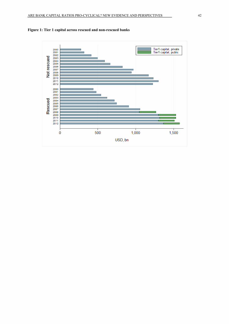
ARE BANK CAPITAL RATIOS PRO-CYCLICAL? NEW EVIDENCE AND PERSPECTIVES
42
Figure 1: Tier 1 capital across rescued and non-rescued banks

ARE BANK CAPITAL RATIOS PRO-CYCLICAL? NEW EVIDENCE AND PERSPECTIVES
43
Figure 2: The capital ratios across macro regions
Euro Area Other Europe
North America Asia-Pacific
Note: In percentage points. Asia-Pacific indicates AU and JP; Euro area includes AT, BE, DE, ES, FR, IT and NL; North America is CA and US; and Other Europe represents CH, UK, and SE.
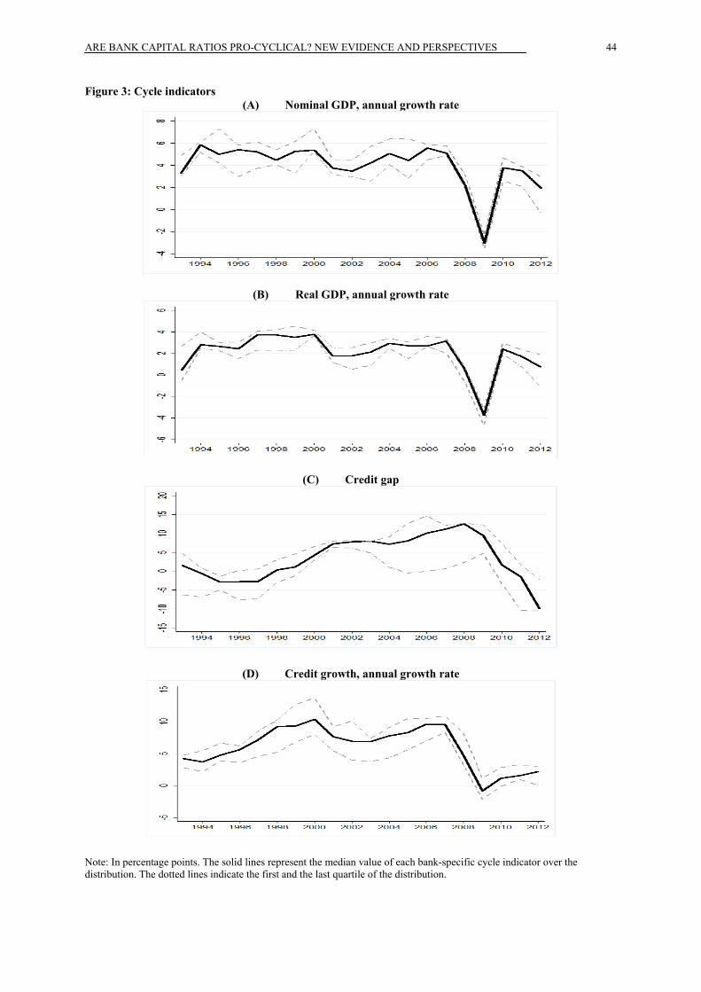
ARE BANK CAPITAL RATIOS PRO-CYCLICAL? NEW EVIDENCE AND PERSPECTIVES
44
Figure 3: Cycle indicators (A) Nominal GDP, annual growth rate
(B) Real GDP, annual growth rate
(C) Credit gap
(D) Credit growth, annual growth rate
Note: In percentage points. The solid lines represent the median value of each bank-specific cycle indicator over the distribution. The dotted lines indicate the first and the last quartile of the distribution.
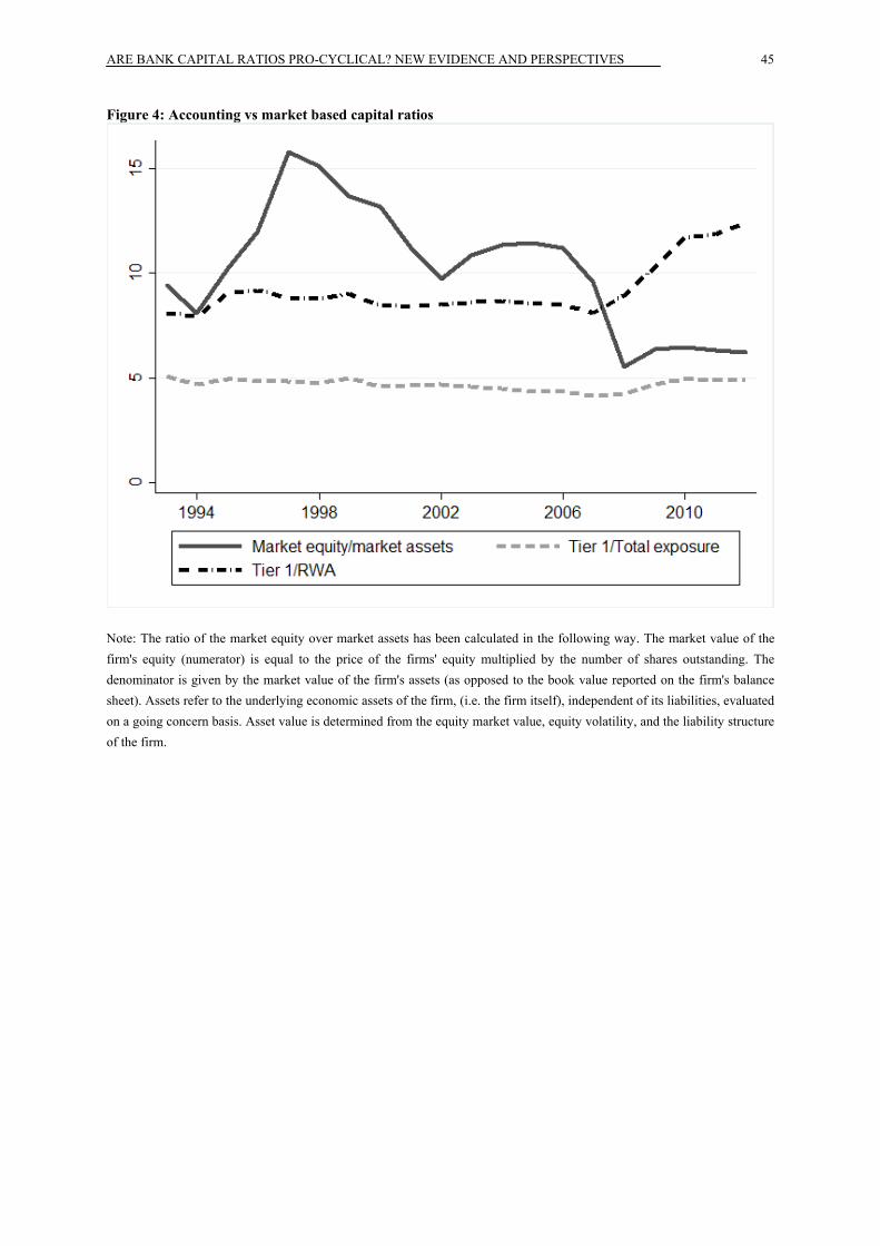
ARE BANK CAPITAL RATIOS PRO-CYCLICAL? NEW EVIDENCE AND PERSPECTIVES
45
Figure 4: Accounting vs market based capital ratios
Note: The ratio of the market equity over market assets has been calculated in the following way. The market value of the firm's equity (numerator) is equal to the price of the firms' equity multiplied by the number of shares outstanding. The denominator is given by the market value of the firm's assets (as opposed to the book value reported on the firm's balance sheet). Assets refer to the underlying economic assets of the firm, (i.e. the firm itself), independent of its liabilities, evaluated on a going concern basis. Asset value is determined from the equity market value, equity volatility, and the liability structure of the firm.

ARE BANK CAPITAL RATIOS PRO-CYCLICAL? NEW EVIDENCE AND PERSPECTIVES
46
Appendix A: How to calculate a proxy for the “exposure measure”.
The new Basel III leverage ratio is calculated as Tier 1 capital over the exposure measure. The exposure measure for the leverage ratio generally follows the accounting measure, according to the following general principles:
on-balance sheet, non-derivative exposures are included in the “exposure measure” net of specific provisions and valuation adjustments (eg credit valuation adjustments);
netting of loans and deposits is not allowed; and
physical or financial collateral, guarantees or credit risk mitigation purchased are not allowed to reduce on-balance sheet exposures.
The Basel III framework provides specific treatments for derivatives, securities financing transactions (SFTs) and off-balance sheet items.
In particular, a bank’s exposure measure is the sum of: (a) on-balance sheet exposures (other than SFTs and derivatives); (b) derivatives exposures; (c) SFT exposures; and (d) other off-balance sheet exposures. This makes the “exposure measure” different from the “total asset” measure, generally used to calculate the denominator of the (accounting) leverage ratio. This is further complicated by the fact that accounting rules in some countries differ significantly and not all the information is available on-balance sheet. For example, derivatives positions are included at the gross level (both among assets and liabilities) using IFRS and directly at the net level using US GAAP.
BankScope data do not have a sufficient level of detail to reconstruct directly a bank’s “exposure measure”.16 However, the high level of detail of the information derived from the Quantitative Impact Study of the Basel Committee on Banking Supervision (QIS database, BCBS (2013)) allows us to calculate coefficients of correction to be applied to BankScope items to “proxy” the effect of the Basel III methodology. Confidentiality issues do not allow us to reconstruct the coefficients of correction at the bank level but only at the country level. Therefore we can correct balance sheet items – on average – for differences in accounting measures across countries but we cannot capture bank-specific heterogeneities. Another important caveat is that QIS data are only available for the period 2011–12 so that, to correct data backward, one has to rely on the (strong) hypothesis that applicable accounting rules have not changed through time.
In particular, we use the following formula to proxy the “exposure measure” (BankScope item codes are indicated in brackets, while the cells of the reconciliation templates used for the correction coefficients are indicated after the acronym “LR”). The rationale of the formula below is to start with the (accounting) measure of total assets and to add/subtract correction components.
Exposure measure=
Total assets (11350) +
Asset derivatives (11160) * (A+B) +
Reverse repos and cash collateral (11145) * C +
[Other off-balance sheet exposure to securitisation (18310) + Acceptances and documentary credits reported off-balance sheet (18320) + Committed credit lines (18325)] * D +
Guarantees (18315) – Goodwill (11300) – Other intangibles (11310) +
16 BankScope moved in 2009 from reporting three spreadsheets for bank analysis (global, liquidity, and universal format) to a universal spreadsheet (Fitch Ratings (2009)). It appears that some items from the off-balance sheet and regulatory capital sections have not been carried over historically for certain banks to the new universal spreadsheet and, thus, we complement the information using the global and liquidity format of historical, archived BankScope releases. Moreover, in some particular cases the information on the two mentioned sections is missing, although it is reported in the years before and thereafter. In these cases, we use information from banks’ published annual reports and, if we do not find any information, we interpolate linearly the items concerned for a maximum of four years.
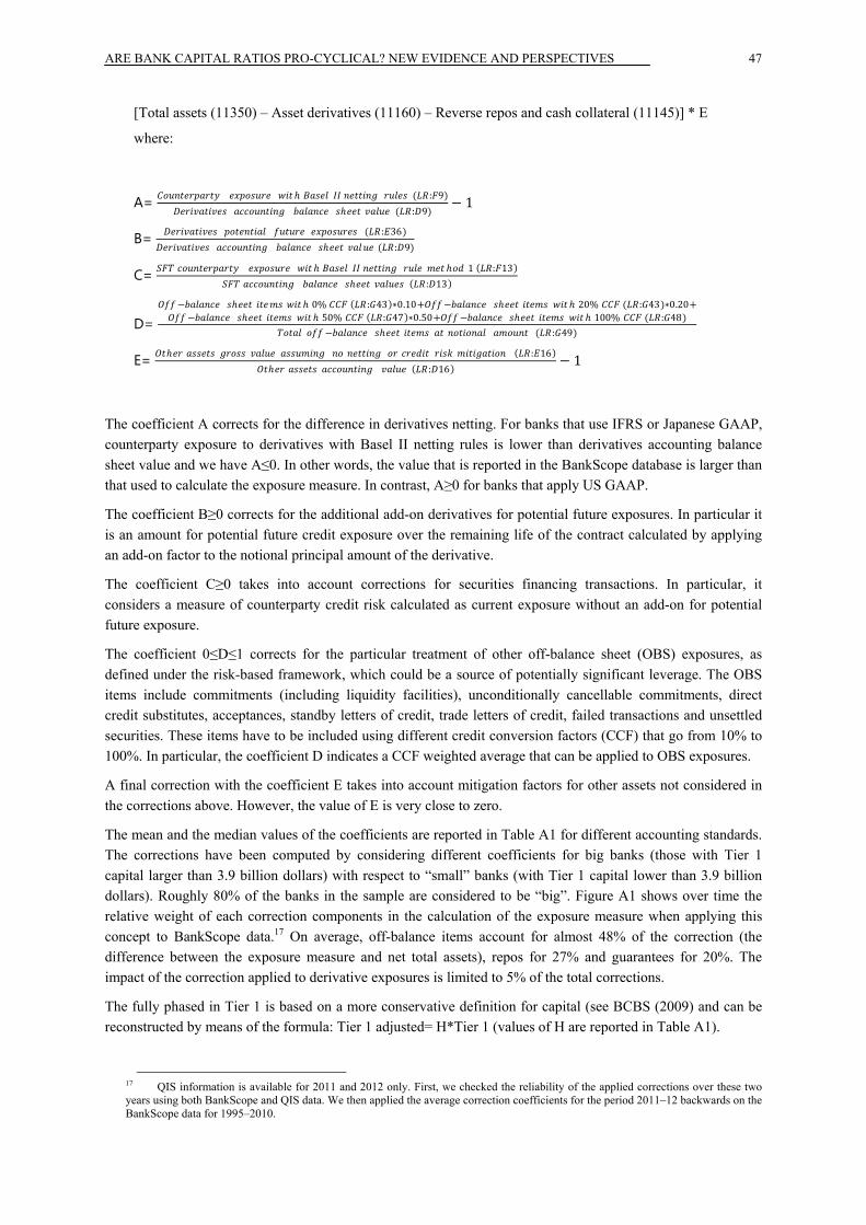
ARE BANK CAPITAL RATIOS PRO-CYCLICAL? NEW EVIDENCE AND PERSPECTIVES
47
[Total assets (11350) – Asset derivatives (11160) – Reverse repos and cash collateral (11145)] * E
where:
A= ℎ ( : 9) ℎ ( : 9) − 1
B= ( : 36) ℎ ( : 9) C= ℎ ℎ 1 ( : 13) ℎ ( : 13)
D= − ℎ ℎ 0% ( : 43)∗0.10+ − ℎ ℎ 20% ( : 43)∗0.20+− ℎ ℎ 50% ( : 47)∗0.50+ − ℎ ℎ 100% ( : 48) − ℎ ( : 49)
E= ℎ ( : 16)ℎ ( : 16) − 1
The coefficient A corrects for the difference in derivatives netting. For banks that use IFRS or Japanese GAAP, counterparty exposure to derivatives with Basel II netting rules is lower than derivatives accounting balance sheet value and we have A≤0. In other words, the value that is reported in the BankScope database is larger than that used to calculate the exposure measure. In contrast, A≥0 for banks that apply US GAAP.
The coefficient B≥0 corrects for the additional add-on derivatives for potential future exposures. In particular it is an amount for potential future credit exposure over the remaining life of the contract calculated by applying an add-on factor to the notional principal amount of the derivative.
The coefficient C≥0 takes into account corrections for securities financing transactions. In particular, it considers a measure of counterparty credit risk calculated as current exposure without an add-on for potential future exposure.
The coefficient 0≤D≤1 corrects for the particular treatment of other off-balance sheet (OBS) exposures, as defined under the risk-based framework, which could be a source of potentially significant leverage. The OBS items include commitments (including liquidity facilities), unconditionally cancellable commitments, direct credit substitutes, acceptances, standby letters of credit, trade letters of credit, failed transactions and unsettled securities. These items have to be included using different credit conversion factors (CCF) that go from 10% to 100%. In particular, the coefficient D indicates a CCF weighted average that can be applied to OBS exposures.
A final correction with the coefficient E takes into account mitigation factors for other assets not considered in the corrections above. However, the value of E is very close to zero.
The mean and the median values of the coefficients are reported in Table A1 for different accounting standards. The corrections have been computed by considering different coefficients for big banks (those with Tier 1 capital larger than 3.9 billion dollars) with respect to “small” banks (with Tier 1 capital lower than 3.9 billion dollars). Roughly 80% of the banks in the sample are considered to be “big”. Figure A1 shows over time the relative weight of each correction components in the calculation of the exposure measure when applying this concept to BankScope data.17 On average, off-balance items account for almost 48% of the correction (the difference between the exposure measure and net total assets), repos for 27% and guarantees for 20%. The impact of the correction applied to derivative exposures is limited to 5% of the total corrections.
The fully phased in Tier 1 is based on a more conservative definition for capital (see BCBS (2009) and can be reconstructed by means of the formula: Tier 1 adjusted= H*Tier 1 (values of H are reported in Table A1).
17 QIS information is available for 2011 and 2012 only. First, we checked the reliability of the applied corrections over these two years using both BankScope and QIS data. We then applied the average correction coefficients for the period 2011–12 backwards on the BankScope data for 1995–2010.
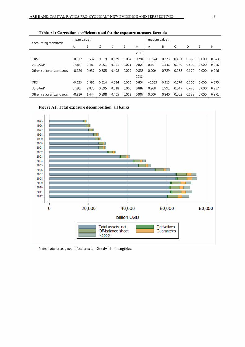
ARE BANK CAPITAL RATIOS PRO-CYCLICAL? NEW EVIDENCE AND PERSPECTIVES
48
Table A1: Correction coefficients used for the exposure measure formula
Accounting standards mean values median values
A B C D E H A B C D E H
2011
IFRS -0.512 0.532 0.519 0.389 0.004 0.794 -0.524 0.373 0.481 0.368 0.000 0.843
US GAAP 0.685 2.483 0.551 0.561 0.001 0.826 0.364 1.346 0.570 0.509 0.000 0.866
Other national standards -0.226 0.937 0.585 0.408 0.009 0.835 0.000 0.729 0.988 0.370 0.000 0.946
2012
IFRS -0.525 0.581 0.314 0.384 0.005 0.834 -0.583 0.313 0.074 0.365 0.000 0.873
US GAAP 0.591 2.873 0.395 0.548 0.000 0.887 0.268 1.991 0.347 0.473 0.000 0.937
Other national standards -0.210 1.444 0.298 0.405 0.003 0.907 0.000 0.840 0.002 0.333 0.000 0.971
Figure A1: Total exposure decomposition, all banks
Note: Total assets, net = Total assets – Goodwill – Intangibles.
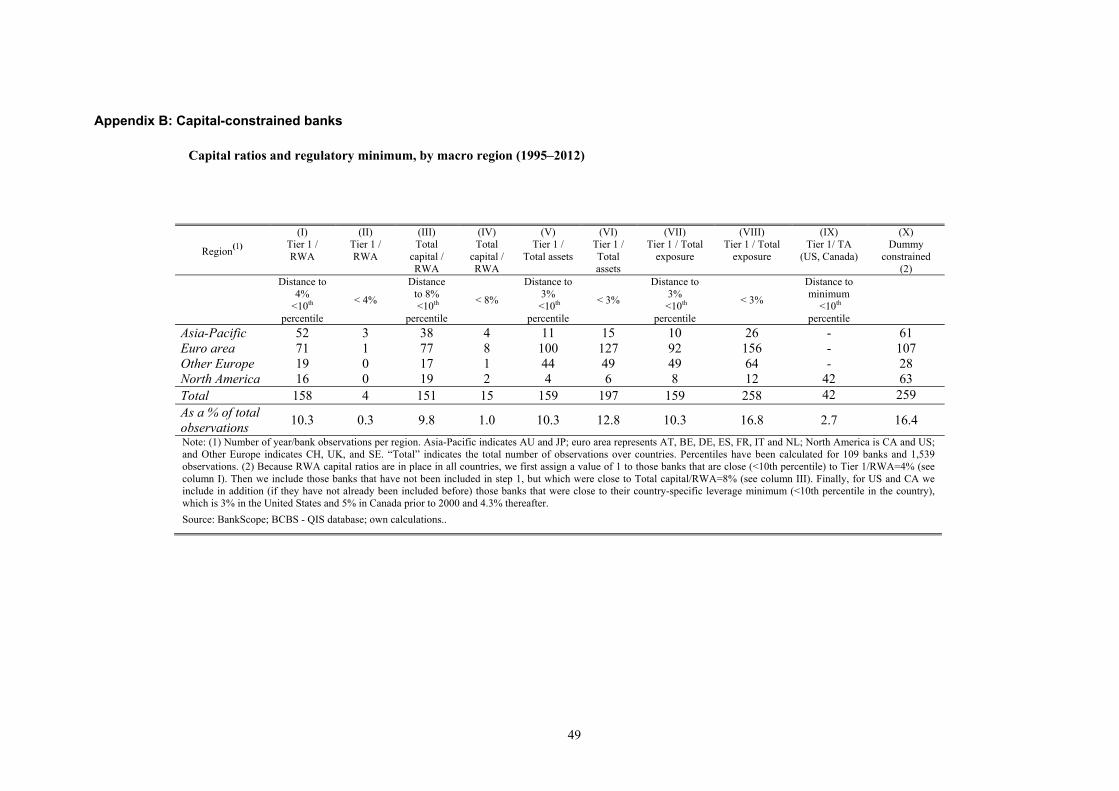
49
Appendix B: Capital-constrained banks
Capital ratios and regulatory minimum, by macro region (1995–2012)
Region(1)
(I) Tier 1 / RWA
(II) Tier 1 / RWA
(III) Total
capital / RWA
(IV) Total
capital / RWA
(V) Tier 1 /
Total assets
(VI) Tier 1 / Total assets
(VII) Tier 1 / Total
exposure
(VIII) Tier 1 / Total
exposure
(IX) Tier 1/ TA
(US, Canada)
(X) Dummy
constrained (2)
Distance to 4%
<10th percentile
< 4%
Distance to 8% <10th
percentile
< 8%
Distance to 3%
<10th percentile
< 3%
Distance to 3%
<10th percentile
< 3%
Distance to minimum
<10th percentile
Asia-Pacific 52 3 38 4 11 15 10 26 - 61 Euro area 71 1 77 8 100 127 92 156 - 107 Other Europe 19 0 17 1 44 49 49 64 - 28 North America 16 0 19 2 4 6 8 12 42 63 Total 158 4 151 15 159 197 159 258 42 259 As a % of total observations 10.3 0.3 9.8 1.0 10.3 12.8 10.3 16.8 2.7 16.4 Note: (1) Number of year/bank observations per region. Asia-Pacific indicates AU and JP; euro area represents AT, BE, DE, ES, FR, IT and NL; North America is CA and US; and Other Europe indicates CH, UK, and SE. “Total” indicates the total number of observations over countries. Percentiles have been calculated for 109 banks and 1,539 observations. (2) Because RWA capital ratios are in place in all countries, we first assign a value of 1 to those banks that are close (<10th percentile) to Tier 1/RWA=4% (see column I). Then we include those banks that have not been included in step 1, but which were close to Total capital/RWA=8% (see column III). Finally, for US and CA we include in addition (if they have not already been included before) those banks that were close to their country-specific leverage minimum (<10th percentile in the country), which is 3% in the United States and 5% in Canada prior to 2000 and 4.3% thereafter. Source: BankScope; BCBS - QIS database; own calculations..