Arctic sea ice leads from advanced very high …psc.apl.washington.edu/lindsay/pdf_files/Lindsay 1995 JGR...with the advanced very high resol.ution radiometer (AVHRR). Although typical

JOURNAL OF GEOPHYSICAL RESEARCH, VOL. 100, NO. C3, PAGES 4533-4544, MARCH 15, 1995

Arctic sea ice leads from advanced very high resolution radiometer images

R. W. Lindsay and D. A. Rothrock

Polar Science Center, Applied Physics Laboratory, College of Ocean and Fishery Sciences University of Washington, Seattle

Abstract. A large number of advanced very high resolution radiometer (AVHRR) images from throughout 1989 are analyzed to determine lead characteristics. The units of analysis are square 200-km cells, and there are 270 such cells in the data set. Clouds are masked manually. Leads are determined from images of the potential open water/5, a scaled ver- sion of the surface temperature or albedo that weights thin ice by its thermal or brightness impact. The lead fraction is determined as the mean/5; the monthly mean lead fraction ranges from 0.02 in winter to 0.06 in summer in the central Arctic and is near 0.08 in the winter in the peripheral seas. A method of accounting for lead width sampling errors due to the finite sample areas is introduced. In the central Arctic the observed mean lead width for a threshold of/5 = 0.1 ranges from 2 or 3 km (near the resolution of the instrument) in the winter to 6 km in the summer. In the peripheral seas it is about 5 km in the winter. Width distributions are often more heavily weighted in the tail than exponential distributions and are well approximated by a power law. The along-track, number density power law N = aw -t' has a mean exponent of b = 1.60 (standard deviation 0.18) and shows some seasonal variability. Mean floe widths in the central Arctic are 40 to 50 km in the winter, dropping to about 10 km in the summer. For floes the power law has a mean exponent of 0.93 and exhibits a clearer annual cycle. Lead orientation is determined with a method based on the direction of maximum extent.

1. Introduction

Leads are a dominant feature in most clear satellite

images of pack ice, appearing as long, jagged, roughly linear features extending from a few to many hundreds of kilometers. Surface observations show that these features

are associated with areas of open water and thin ice whose widths vary from a few meters to many kilometers. Many of these leads are easily distinguished in images acquired with the advanced very high resol.ution radiometer (AVHRR). Although typical lead widths are less than the nominal 1.1-km resolution of the instrument, the high thermal and brightness contrast between the cold, bright floes and warm, dark leads allows them to be easily observed in almost any cloud-free image obtained with AVHRR. Thus we can observe many subpixel-sized leads in AVHRR images owing both to this high contrast and to the characteristic network like patterns of the leads.

Leads are intimately tied to the heat and momentum bal- ance of sea ice. The atmospheric turbulent sensible heat flux in winter, for example, is typically downward and of the order of 10 W m '2 over floes but is large and upward over leads to such an extent that the average flux over leads and floes is often upward and also of the order of 10 W m '2. The inclusion of this large lead effect is a topic of current interest for climate modelers who wish to treat the

Copyright 1995 by the American Geophysical Union.

Paper number 94JC02393. 0148-0227/95/94JC-02393 $05.00

ice cover as simply as possible while retaining the crucial physics. Leads have similarly important effects on the net radiative flux. Leads are also clearly related to past ice deformation in ways not much explored. Lead patterns and orientations are thought to be connected with the stress- strain relationship for the ice pack and to the way the pack interacts with the coast.

In spite of their relevance there are few observations of the geometric properties that describe lead and floes. There is certainly nothing that we could hold out as a climatology of lead properties. How do they vary throughout the year and by region? There are no numbers obtained from any broad observational program that could be used as inputs for or a check of climate models. Although the present study is not a climatology, representing but a single year, we present some averages of lead properties that show how a useful climatology might be constructed.

Although we all would claim to know a lead when we see one, there is no generally accepted definition of a lead, and the concept remains ambiguous. In one context a lead may imply open water; in another, ice too thin to cross; and in yet another, any first-year ice that is thermally or visually distinguishable from the rest of the ice pack. We use a concept of potential open water and a fixed threshold of this quantity to provide a somewhat uniform definition of leads that is based on thermal and visible radiometric

properties and not on geometric properties or spatial image processing techniques. This is an attempt to standardize what is called a lead in scenes of quite different mean temperatures, reflectances, and lighting conditions.

Here we summarize some of the information that can be obtained about leads from AVHRR thermal and reflected

4533

4534 LINDSAY AND ROTHROCK: LEADS FROM AVHRR

solar channels and show results from images collected throughout a full year. The average values of the effective lead fraction, determined from the mean potential open water, are shown, as well as the average lead fractional area for different thresholds. A method to determine lead

and floe widths is described, and a correction for sampling error is introduced. The mean lead widths and floe widths

are shown, and both the lead width and the floe width distributions are found to approximate power laws. Finally, the lead orientation is investigated using a method based on the direction of maximum extent.

2. Data Preparation

The AVHRR is an imaging instrument that flies on the National Oceanic and Atmospheric Administration (NOAA) series of polar-orbiting satellites. Two NOAA satellites are in orbit at a time, each observing the polar regions up to 14 times a day. AVHRR has five channels as follows: two at•eflected solar wavelengths (channel 1 at 0.58 to 0.68 gm and channel 2 at 0.72 to 1.10 gm), two at thermal infrared wavelengths (channel 4 at 10.3 to 11.3 gm and channel 5 at 11.5 to 12.5 gm, although in even-num- bered satellites, channel 5 is a repeat of channel 4), and one that is sensitive to a combination of emitted thermal

and reflected solar energy (channel 3 at 3.55 to 3.93 gm). The description and specifications of the AVHRR instrument are given by Kidwell [1991]. The AVHRR sensor has been routinely used to observe ice extent and, usually by manual interpretation, ice type. Ice centers around the world consult it on a daily basis to determine the ice edge and to estimate the ice concentration.

The geolocation and calibration of the images used in this study were performed at the Naval Research Laborao tory (NRL) [Fetterer and Hawkins, 1991]. Relatively cloud-free images taken by NOAA 10 and NOAA 11 throughout 1989 were selected for temporal and regional coverage from hard-copy prints provided by the National Ice Center. Level lB digital tapes were then obtained from the National Environmental Satellite Data Information Ser-

vice (NESDIS). The images are mapped to a 1.0-km grid using a polar stereographic projection true at 70øN and nearest neighbor interpolation. The complete set of 248 images processed by NRL for 1989 is available from the National Snow and Ice Data Center. Unfortunately, this data set does not include May, an important transition month.

No reliable automated cloud-masking procedure is pres- ently available for AVHRR scenes over pack ice, although there is much active research on the problem [e.g., Key and Barry, 1989; Ebert, 1989; Rossow, 1989; Welch et al., 1992]. We use an interactive procedure based on manual interpretation of the images and scattergrams of channel pairs and channel differences. All five channels are used when available. Shore leads and land are also included within the cloud masks.

The unit of our analysis is the cloud-free portion of a 200-km square "cell." These cells have been selected as relatively cloud-free areas of 512-km square regions that have been cloud masked. Individual cells may be as little as one third cloud free owing to the very small size of many of the holes in the clouds, especially in the summer. Both the surface temperature and the surface albedo are

estimated for the cloud-free portion of each cell. Thermal analysis of leads is restricted to the months during which there is a significant thermal contrast between leads and thick ice (all but June, July, and August), and we have restricted our albedo analysis to cells for which the sun is more than 10 ø above the horizon (limiting albedo estimates to March through September). The locations of all 270 cells analyzed are shown in Figure 1. In our subsequent analysis, cells are identified as being within either the central Arctic (127 cells) or the peripheral seas (143 cells); the line between them corresponds roughly to the minimum extent of multiyear ice.

The ice surface temperature used here is estimated from channels 4 and 5 using a "split window" algorithm devel- oped specifically for Arctic sea ice [Key and Haefiiger, 1992]. It is based on a radiometric model of the atmosphere applied to temperature and humidity data from radiosonde profiles obtained from former Soviet Union ice camps. The surface temperature Tsfc is estimated as

T•fc = ao + a4T4 + a5 T5 + a45(T4-Ts) sec • (1)

Here, T4 and T5 are the channel 4 and 5 brightness temperatures in degrees Kelvin, • is the scan angle (angle from nadir measured at the satellite), and ao, a4, as, and a45 are coefficients determined for each of three seasons (winter, transition, and summer) and for each of three satellites (NOAA 7, 9, and 11). An analysis of the surface temperature of sea ice and procedures for estimating the sensible heat flux from leads in the Arctic based on the 1989 NRL

data set is given by Lindsay and Rothrock [1994a]. Largely because of imperfect cloud masking and undetect- able ice crystal precipitation, the surface temperature esti- m/•ted from (1) has an rms error of 2.7 K compared with air temperatures measured at drifting buoys and manned stations [Yu et al., this issue].

Central Arctic Peripheral seas

Figure 1. Map of cell locations Each cell measures 200 km square.

from throughout 1989.

LINDSAY AND ROTHROCK: LEADS FROM AVHRR 4535

The albedo is determined with a seven-step process as outlined by Lindsay and Rothrock [1994b]. To estimate the surface albedo, defined here as the hemispherically and spectrally averaged fraction of the clear sky solar flux reflected by the surface, we must (1) obtain digital counts from the NRL values, (2) determine the narrowband radi- ance using Current estimates of the instrument's gain, (3) calculate the top-of-the-atmosphere reflectance of a Lam- bertian surface, (4) account for the nonisotropic reflectance of the ice and atmosphere, (5) correct for atmospheric interference, (6) convert the narrowband (channel) reflectance to a broadband albedo, and (7) normalize to a common solar zenith angle of 70 ø . Comparisons with the few other data available suggest that the albedo, determined in this manner, has a standard error of about 0.10.

Because of the variable resolution of the data across the

image swath, the statistics calculated from the images are sensitive to the distance from the nadir line. We have lim-

ited our analysis to cross-track scan angles less than 45% where the along-track resolution is 2.3 km ahd the cross- track resolution is 3.1 km.

3. Lead Definition: Potential Open Water

The problem of lead definition is critical in any remote sensing analysis of lead properties. Leads can be determined with edge detection algorithms, but the geophysical significance of such leads is uncertain. Leads can also be determined by a combination of a threshold and spatial properties, but, again, geophysical interpretation is uncertain. Another approach to defining leads is to look for a bimodal distribution of temperature (or brightness) and pick a value between the modes as a threshold between "leads" and "thick ice" [Key and Peckham, 1991; Kittler and lllingworth, 1986; BanfieM, 1992]. This procedure is not robust when used with AVHRR data because there are

seldom two distinct modes in the temperature or albedo distributions. This is due, in part, to the low resolution of the instrument compared with the size of the leads, so that many pixels are "mixed" and, in part, to the variability of the temperature and albedo of floes as discussed below.

We choose to define leads in terms of their observed

thermal and brightness levels. We use the concept of potential open water to estimate the total impact of both open water and thin ice and then use a threshold for potential open water to define leads. Potential open water is simply an ad hoc way to normalize or standardize what is defined as a lead in all scenes by their individual thermal and brightness levels.

We define potential open water õ as the fraction of a pixel that must be open water for it to have the observed temperature or albedo if the pixel is composed of some mixture of open water and thick ice. The fraction õ ranges between zero for a pixel composed only of cold or bright thick ice and unity for a pixel at the temperature or brightness of open water. This is a natural mapping of temperature or albedo because if the leads are composed of open water, then the lead fraction in mixed pixels results. We first define õ in terms of temperature. The surface temperature Tsfc is estimated for each pixel with the Key and Hae- fiiger [1992] algorithm; Tt, is the background temperature of the thick ice, and the temperature of open water Tow is

fixed at-1.8øC. The potential open water based on temperature is then

15 T = rsfc-Tb ro w _ rt ' , > (2)

8 T = 0, Tsfc < Tt,. (3)

The background temperature represents the temperature of the floes and is considered to be a smooth temperature field that varies slowly across a cell. The background temperature is taken as an approximation of the temperature of the coldest quartile of the surface temperature distribution. The value of the potential open water is not very sensitive to the order statistic (e.g., tenth percentile or quartile) chosen for the background because the width of the temperature distribution is commonly small compared with the difference in temperature between most of the ice and open water. The quartile value is chosen over, say, the median, so that small areas within a cell may contain large areas of leads, up to 75%, and the background value will be left unaffected.

The 200-km cells often support a substantial horizontal temperature gradient, which is interesting as part of the synoptic (low wavenumber) temperature field but needs to be removed to distinguish the synoptic temperature variation from the temperature contrast between leads and floes. We estimate the background temperature then as a bilinear function

T• = a x + b y + c. (4)

A cell is divided into nine equal subregions, of which at least five must be at least 50% cloud free for the cell to be

retained in the data set. For each subregion we find T25, defined as the 25th percentile of the temperatures of the cloud-free pixels and the median location (x, y) of these pixels. These five to nine values of T25 and their locations are used to evaluate the coefficients in (3) by least squares regression. The bilinear trend removal is a simple and robust method of accounting for the changes in the background temperature across a cell. It accommodates the irregularly shaped, cloud-free regions well, does not suffer the instabilities of higher-order methods, and is cleaner to implement on irregular cloud-free regions than Fourier methods.

The low variability of the surface temperature in the summer makes õr poorly defined, but then there is high contrast in the albedo. For potential open water based on albedo we use a definition similar to that for temperature

(Z b - (Zsf c - (5) •SA - Ot b_ Otow

The estimated albedo of the ice surface at each pixel is 0tsfc, the background albedo (defined in a manner similar to that of temperature but as the brightest quartile) is 0t0, and the albedo of open water (taken as 0.10) is 0to• In our analysis of lead and floe widths, õr is used for all months, except June, July, and August, when õA is used.


This definition of potential open water is similar to the tie-point technique that uses visible wavelengths to determine ice concentration in summer [Comiso and Zwally, 1982; Steffen and Schweiger, 1990; Burns et aL, 1992]. In these studies the ice pack is assumed to consist of either thick ice or open water, with no thin ice present; otb is chosen from bright floes, and 1-õA is used as an estimate of ice concentration. For the cold seasons, 8T or õA is more useful than open water concentration if a single number is desired to represent the fraction of thin ice and open water, since thin ice is weighted by its thermal (or brightness) impact. The parameter õ is consistently greater than an estimate of open water only, since thin ice is included and considered to be made up of proportions of thick ice and open water. Because of the linear nature of its definition, the mean value of õ is not strongly influenced by the resolution of the instrument; a higher resolution instrument would better define the tails of the distribution and would

undoubtedly find higher maximum values of õ, but the mean over a cell would remain the same.

The mean values of •5 determined from albedo and from

temperature data are well correlated. The squared correla- tion is 0.87 over 64 spring and fall cells in which the mean temperature is less than -10øC. There is a small bias, with mean õ• values averaging 10% higher than mean 8T values. This bias cannot be extrapolated to the summer, when there is little thermal contrast. The bias reflects the nonlin-

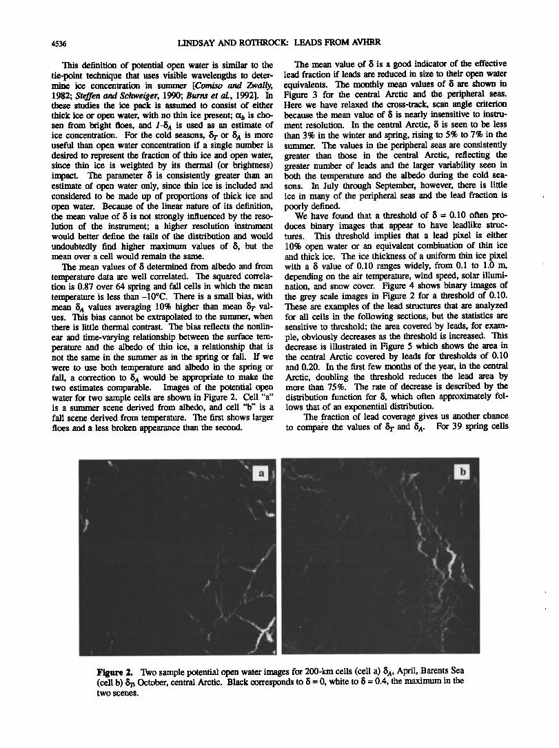
ear and time-varying relationship between the surface temperature and the albedo of thin ice, a relationship that is not the same in the summer as in the spring or fall. If we were to use both temperature and albedo in the spring or fall, a correction to 8A would be appropriate to make the two estimates comparable. Images of the potential open water for two sample cells are shown in Figure 2. Cell "a" is a summer scene derived from albedo, and cell "b" is a fall scene derived from temperature. The first shows larger floes and a less broken appearance than the second.

The mean value of 8 is a good indicator of the effective lead fraction if leads are reduced in size to their open water equivalents. The monthly mean values of õ are shown in Figure 3 for the central Arctic and the peripheral seas. Here we have relaxed the cross-track, scan angle criterion because the mean value of õ is nearly insensitive to instrument resolution. In the central Arctic, õ is seen to be less than 3% in the winter and spring, rising to 5% to 7% in the summer. The values in the peripheral seas are consistently greater than those in the central Arctic, reflecting the greater number of leads and the larger variability seen in both the temperature and the albedo during the cold seasons. In July through September, however, there is little ice in many of the peripheral seas and the lead fraction is poorly defined.

We have found that a threshold of õ = 0.10 often pro- duces binary images that appear to-have leadlike structures. This threshold implies that a lead pixel is either 10% open water or an equivalent combination of thin ice and thick ice. The ice thickness of a uniform thin ice pixel with a õ value of 0.10 ranges widely, from 0.1 to 1.0 m, depending on the air temperature, wind speed, solar illumi- nation, and snow cover. Figure 4 shows binary images of the grey scale images in Figure 2 for a threshold of 0.10. These are examples of the lead structures that are analyzed for all cells in the following sections, but the statistics are sensitive to threshold; the area covered by leads, for example, obviously decreases as the threshold is increased. This decrease is illustrated in Figure 5 which shows the area in the central Arctic covered by leads for thresholds of 0.10 and 0.20. In the first few months of the year, in the central Arctic, doubling the threshold reduces the lead area by more than 75%. The rate of decrease is described by the distribution function for 8, which often approximately follows that of an exponential distribution.

The fraction of lead coverage gives us another chance to compare the values of • and 8A. For 39 spring cells

a

Figure 2. -Two sample potential open water images for 200-km cells (cell a) 8 A, April, Barents Sea (cell b) •, October, central Arctic. Black corresponds to õ = 0, white to 15 = 0.4, the maximum in the two scenes.


ß Central Arctio

ß Peripheral seas

'A

r

ß

ß .... &..-'

• I I I I I I I I I I I I ß

o Jan Mar May Jul Sep Nov

Figure 3. Monthly mean potential open water based on temperature for all months, except June and August, when albedo is used. There was an average of 22 cells in each month for the central Arctic and 17 cells each month for the

peripheral seas. Some months had fewer than four cells and are not plotted.

the median ratio of (area fraction of õA) / (area fraction of õt) is 1.00 at a threshold of õ = 0.10 and 1.09 at õ = 0.20, indicating that at the lower threshold, õr and õA show similar concentrations of leads, but at the higher threshold, appropriate for the hotter and darker lead areas, õA shows a larger concentration. This may be related to the fact that very thin ice is relatively dark, yet can support a large temperature differential between the top and bottom surfaces.

4. Lead and Floe Width Distributions

The lead and floe width distributions for each cell are

determined with a series of 200 randomly placed and randomly oriented transects. Each transect is followed from one edge of the image to another with areas of cloud mask, taken as missing dataß Each random transect is followed in 1.0-km steps; at each step the nearest pixel is determined

ß POW = 0.1 ß ß POW = 0.2 -

.

A• •"• ' 4'--;-'-; I I I I I I I i i

Jan Mar May Jul Sep Nov

Figure 5. Mean area covered by leads when using õ thresholds of 0.10 and 0.20 for the central Arctic only. There was an average of 11 cells each month.

and the corresponding õ value is found. A single lead width is determined by the length of the transect for which the õ value remains above the chosen threshold; a floe width is just the length of the transect below the threshold and might also be called the lead separation distance. The widths w of individual leads or floes are determined to the

nearest 1 km, corresponding to the grid size of the geolo- cated images, and in this manner, histograms of the lead and floe widths are established.

The transect method is 'easily implemented and does not depend on defining leads as objects. In addition, winds, survey aircraft, and submarines commonly encounter leads at random angles, so our technique mimics these encoun- ters. Lead width statistics estimated from random transects

are more directly compared with aircraft and submarine transects and are more directly applicable to sensible heat flux estimates, in which the lead width experienced by the wind plays a role. These widths are random "chord" widths and not perpendicular crossing widths as discussed

Figure 4. Binary images of the two cells in Figures 2a and 2b showing leads with õ values above 0.10.


by Key and Peckham [1991], who present a method for determining the perpendicular crossing width distribution from a transect width distribution that includes the effects

of a dominant lead orientation. Lead properties can also be determined from morphological models based on skele- tons. Banfield [1992] uses this technique to assess lead length, area, width, and orientation for synthetic aperture radar (SAR) images of leads.

A serious bias can be encountered in the distributions

by using a finite area for sampling, in that large leads or floes that intersect the edge of the image (or a cloud bank) are not completely sampled. The theory of censored data

_

analysis offers a correction for this problem. The discussion that follows is couched in terms of leads, but the treat- ment of floes is identical. Fully and partially observed leads are counted separately. If a lead is not interrupted by cloudy areas or the edge of the cell, then it is taken as fully observed, and the histogram bin of fully observed leads corresponding to the observed length is incremented by one. If the lead is interrupted by clouds or by the image edge, then the histogram bin of partially observed leads corresponding to the observed length is incremented. Histo- grams of lead sizes are determined from 1 km to the maximum size observable, W = 280 km, the diagonal width of the cell. For all 200 transects combined, we define

Nl(w) as the total number of fully observed leads of transect width w and Np(w) as the total number of partially observed leads of observed transect width w. The leads

that are partially observed are known to have a width greater than or equal to w. Our problem then is to determine an unbiased estimate of the discrete probability distribution function (pdf) of the lead widths:

f(w) = P(lead width = w) (6)

Note that f(w) is the pdf for lead widths, given that a lead is either fully or partially observed.

Following the method of Cox and Oakes [1984, p. 56], we can write the Kaplan-Meier or product limit estimator F(w) of the cumulative distribution function (cdf) giving the proportion of leads greater than or equal to width w as

r(k) k<w

(7)

where r(k) is the adjusted number of leads or floes greater than or equal to width k

r(k) = Z [Nf(w) +%(w)] -2 P(k) (8) w=k

The adjustment 1/2 N•,(k) is needed to account for the discrete representation of a continuous distribution function. The discrete probability distribution is then

f(w) = F(w) - F(w+l) (9)

From this the corrected mean and variance of the size distribution are

W

- z w = w f(w) (10) w=l

and

w

2 • (w- Vo) 2 f(w) (11) (•w = w=l

The edge correction procedure causes both the mean and the variance to be greater than those found by treating both fully and partially observed leads alike. For a threshold of õ = 0.1 the mean widths increase an average of 25% for both leads and floes. The Kaplan-Meier method is non- parametric and as such does not assume a form for the distribution. The analysis of the lead and floe widths that follows includes these corrections for censored data.

The lead and floe widths can be described either in

terms of their number density distribution f(w) or their fractional area distribution fA(W) = (area covered by leads of width w) / (total lead area). If we assume that fractional area is well sampled by the fractional length measurements of the transect method, then the translation between them is simply

= wZ(w) = wZ(w) fA(w) Zwf(w) •

(12)

Many applications may find it more useful to use the fractional area distribution.

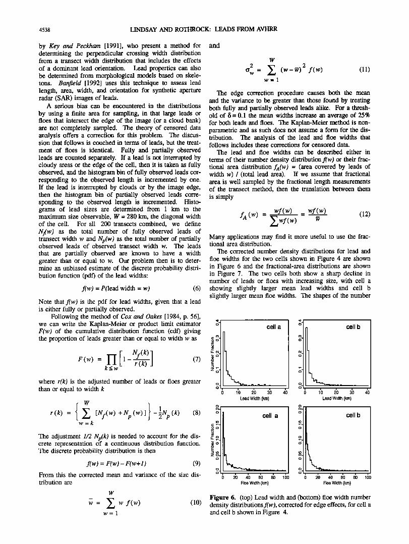
The corrected number density distributions for lead and floe widths for the two cells shown in Figure 4 are shown in Figure 6 and the fractional-area distributions are shown in Figure 7. The two cells both show a sharp decline in number of leads or floes with increasing size, with cell a showing slightly larger mean lead widths and cell b slightly larger mean floe widths. The shapes of the number

cell a

• i• _ I.L_ i-• _

0 1'0 2'0 3'0 Lead Width (km)

cell a

0 2'0 4'0 6'0 8b 100 0 20 40 6'0 8b 160 Floe Width (km) Floe Width (km)

• cell b

_ _

!

0 1'0 2'0 3'0 4'0 Lead Width (km)

• cell b I--.

õ.

Figure 6. (top) Lead width and (bottom) floe width number density distributions fiw), corrected for edge effects, for cell a and cell b shown in Figure 4.


O.

1}:)

cell a

Lead Width (kin)

cell a

6 2'0 • 6'0 •0 160 Floe Width (Kin)

i cell b

0 lb 2'o 3'0 4'o Lead Width (kin)

øø' cell b

õ, 4 •'o • •'o do •6o

Floe Width (kin)

Figure 7. (top) Lead width and (bottom) floe width fractional area distributions fA(W), corrected for edge effects, for cell a and cell b shown in Figure 4.

The mean floe widths are also shown in Figure 8. The mean widths are between 40 and 45 km in the central Arc-

tic from January through April, dropping sharply to nearly 10 km in the summer and then rising through the fall to nearly 40 km again in December. They are about half as big in the peripheral seas. The floe widths would be smaller for lower thresholds of f)Z, since "colder" leads can then appear to break large floes.

A simple, one-parameter model of the number density lead width distribution is the exponential

1 -w/X. f(w) = •e (13)

where the single parameter • is the mean lead width. Some authors have used this distribution to approximate lead widths [e.g., Key and Peckham, 1991]. The maximum likelihood estimate of • for censored data can be computed directly from the fully and partially observed width distributions without referring to the corrected distribution calculated above [Lawless, 1982]:

W

w + (w) ] w

Nf(w) w=l

(14)

density distributions are roughly exponential, but, as we shall see, a power law is a somewhat better description of the distributionsß Also note that these are distributions of

lead or floe widths given that a lead or floe is observed, and they do not reflect the higher lead fraction seen in cell b.

For the smallest floe sizes the fractional area distribution increases with floe size, in contrast to the general decrease in the fractional area coverage for leads with increasing lead size. (The apparent increase in the lead area from 1 to 2 kms is most likely a result of the coarse resolution of the instrument.) The floe sizes in cell a show little decrease in area with size for floes less than 40 krn in width. The large number of small floes reflects the broken nature of the ice in many lead areas and the very irregular shape of some leads, but their total area is small. The small sample area (2002 km 2) makes the fractional area distribution subject to significant variations for large leads or floes.

The monthly averaged lead widths for all scenes are shown in Figure 8. We see that the lead widths in the cen-

tral Arctic are 2 to 4 km in the winter. The fact that the mean widths are near the limit of the resolution of the instrument reflects the selection of the threshold, since the threshold was determined, in part, by the appearance of the resultant binary images. We sought a level that produced narrow, leadlike structures, as narrow as the resolution would permit. Clearly, AVHRR is not the ideal sensor for measuring lead width statistics. However, for a constant threshold we can make useful intercomparisons between different seasons and different regions. In the central Arc- tic the average lead width stays between 2 and 4 km in all months, except September, when it rises to nearly 7 km. In the peripheral seas the average widths are 4 to 7 km, indicative of the more open nature of the ice in these regions.

ß Central Arctic

ß Peripheral seas

I I I I I

Jan Mar May I I I I I

Jul Sep Nov

Central Arctic

Peripheral seas

I I I I I I I I I I I I

Jan Mar May Jul Sep Nov

Figure 8. Monthly averaged mean (top) lead widths and (bottom) floe widths for a threshold of /5 = 0.10, using distributions corrected for censored data. The parameter fir is used, except for June, July, and August, when õA is used. There was an average of 12 cells per month for both regions.


This is just the total lead length, both fully and partially observed, divided by the number of fully observed leads. The negative-exponential distribution is often thinner in the tail than the observed lead widths. Figure 9 shows the mean width versus the standard deviation for all 102 cold

season cells; for a negative-exponential distribution the two are equal. For cells with large mean widths the standard deviations are substantially larger than what would be expected for the observed mean lead widths, implying that the tails of these distributions are heavier than those of the

negative-exponential distribution. Another possible description of the lead width distribu-

tion is the power law. Wadhan• [1981] and Wadhams et al. [1985] have suggested a power law for the number density of leads found along a submarine track. The resolution of the submarine sonar observations is much finer than

that of the AVHRR observations, about 5 m, and their definition of a lead is ice less than 1.0 m thick. The track num-

ber density Nr(w) is defined as the number of leads of width w per kilometer of track per kilometer of width increment. In terms of both the number density distribution f(w) and the fractional area distribution fA(w),

N (w) _ Nleads f (w) Cf A (w) NT(W) = LA - LA wA (15)

where N(w) is the total number of leads observed of width w, L is the total length of the randomly placed tracks across the image (in kilometers), A is the bin size(1 km), C is the lead concentration, and Nleads = (LC) / W is the total number of leads observed of all sizes. The track num-

ber density Nr(w) has units of inverse kilometers squared. The extension to floes is obvious.

Figure 10 shows a log/log plot of Nr versus w for both leads and floes for the two sample binary image cells in Figure 4. Note the nearly linear trends, yet distinct slopes. The slope is slightly lower (more gradual) for floes, imply-

O -

q- ++ ++ ..-- o

..-"

Mean Lead Width (km)

Figure 9. Standard deviation versus mean lead width for 102 different cold season cells in the central Arctic, corrected for censorship. The standard deviation equals the mean in a negative-exponential distribution.

ing relatively more large floes than large leads. Such log/ log plots for all of the cells were fit with straight lines to determine the parameters a and b in a power law

-b

NT(W ) = aw (16)

for leads up to 20 km and floes up to 30 km in width. The exponent b indicates the relative frequency of large and small leads or floes, while the coefficient a is directly related to the lead or floe concentration C and the range of widths over which the power law is thought to apply. Clearly, the power law can apply only to a limited range of widths.

The shapes of the lead and floe width distributions are highly variable owing both to natural variations in the distributions and to the small sample sizes that the 200-km 2 cells represent. The power law we have described here implies a straight line for a log/log plot of the density distribution versus the lead or floe width. However, most of the lines show a small curvature, commonly negative (concave down). A second-order fit is often significantly better (using a t test) with the additional parameter available in such a fit, but the improvement is not dramatic. In the central Arctic the median value of the explained variances increases from 91% to 92% in going from a linear (log Nr(w) = a - b log w) to a second-order (log Nr(w) = cl + c2 log w + c3 (log w) 2) fit of the track number density. In contrast, the median value for a fit to the exponential distribution is only 81% (log Nr(w) = a - b w). Objective measures of the goodness of fit of the parameterized distributions to the sample distributions, measures that would further evaluate the merits of the first- and second-

order fits, are based on the assumption of independent sam- ples, a condition not met with our sampling scheme of 200 transects in a single cell. While the second-order fits are marginally better than the first-order fits, the summary and the interpretation of the results become much more com- plex. Furthermore, we suspect that the small negative curvature detected in the log/log distributions may reflect the poor resolution of the instrument, leading to an underrepre- sentation of leads only one or two pixels wide compared with those of greater width. For these reasons, we have used the first-order fit in our analysis.

Figure 11 shows monthly averages of the exponent b for leads and floes for cells in the central Arctic and peripheral seas. For leads there is a small seasonal cycle for the central Arctic in the exponent b, with larger values in the summer, implying relatively more large leads. The annual mean is 1.60 (standard deviation 0.18). It shows little change for a higher threshold of õ = 0.20. Wadhams [1981] found a steeper drop in the number of large leads with b = 2 for a 100-m bin width over a range of widths of 50 m to 1.0 km in Fram Strait and north to the North Pole.

In Davis Strait, Wadhams et al. [1985] found-b = 2.29 for a similar bin size and width range. Our bin size and width range are substantially larger, yet a power law still appears to hold. Our larger exponents may be related to the lower resolution of the AVHRR instrument, or they may indicate that the exponent changes with scale.

The exponent b also shows an annual cycle for floes, with a smaller exponent in the summer reflecting the exist- ence of relatively fewer large floes. The annual mean is


\\b

ß

x\

\\ b

aX'x•\

Lead width (km) Floe width (km)

Figure 10. (left) Lead and (right) floe number densities along a track (expressed as the number of leads or floes per kilometer of track per kilometer of width increment) in log/log plots for the two binary images (cells a and b) in Figure 4. The bin size (width increment) is 1 km.

0.93 (standard deviation 0.21). The power law has interesting implications when the exponent is near 1. The fractional area distribution is proportional to W -b'l'l , SO the first derivative is

-b

3•fA (W) • (-b+ 1)w (17)

If b > 1, fA(W) decreases monotonically with w; if b = 1, fA(W) is constant; and if b < 1, it increases. So the average fractional area distribution for floes in the central Arc- tic increases with floe size for all months except August and September, when it decreases.

ß ,• t•. ?. ,

?. o

x

ß Central Arctic

ß Peripheral Seas

ß

leads

'6

• I I I I I I I I I I I I

"' Jan Mar May Jul Sep Nov

ß .... •.-' ß

/

ß I

I I I I

d• M•

ß -.- -.- ß

floes

I I I I I I I I

May Jul Sep Nov Figure 11. Monthly averages of the power law exponent b for (top) leads and (bottom) floes. There was an average of 11 cells each month in the central Arctic and 14 in the

peripheral seas.

5. Lead Orientation

Lead orientations in the pack ice are significant because they both reflect and influence the dynamics of the ice movement. We wish to determine the orientation of the

leads seen in the potential -open water images. There are several ways to measure the orientation, all with their strengths and weaknesses. Possible methods include the local gradient in the image (Sobel operator), the two-dimen- sional Fourier transform, a Hough transform, skeleton orientations, and the direction of maximum extent. Fetterer et al. [1990] used a Hough transform to analyze lead orientation in binary images of sea ice. The technique shows promise but is subject to several arbitrary decisions in order to determine the dominant orientation from the accu-

mulation matrix in the transformed space; it is also sensitive to the shape of the area examined. The Fourier transform works poorly on irregularly shaped regions, which are characteristic of our cloud-masked images. The local gradient operator was found to give noisy and incon- sistent results. The method based on the skeletal analysis of leads was introduced by BanfieM [1992] and includes several measures of orientation. It depends on identifying leads as individual entities. We develop here a method based on the direction of maximum extent of a lead which

is fast, robust, and accurately reflects visual perceptions of lead orientations.

Each lead pixel in a binary image is examined. The length of each line segment passing through the pixel and entirely contained in the lead is determined for all possible orientations (we use tz =-80 ø to +90 ø in 10 ø increments.) The within-lead extent is found by stepping along a line


for each orientation in one pixel steps until the line crosses out of the lead (this criterion is slightly modified by allow- ing for gaps of at most one pixel). The direction of maximum extent is determined, and the corresponding angular bin is incremented by one. (If there is a tie for the maximum length, all of the corresponding bins share the single count equally.) Each lead pixel contributes equally to the angular distribution, yet large leads are weighted heavily because they contain many pixels. Any lead pixel for which any orientation line extends to the edge of the image (or a cloud-masked region) is excluded, as well as pixels that show no clear orientation because the ratio of the max-

imum length to the minimum length is less than 3.0. Finally, the angular distribution is normalized by the total count of valid lead pixels.

The degree of orientation of the leads, most simply seen in the magnitude of the peak of the angular distribution, is a function of the size of the area examined, in that a single lead or system of leads with a specific orientation is more likely to dominate a small image. The results we show here are specific to the 200-km cells we have analyzed. Figure 12 shows the angular distribution of maximum lengths for a sample cell from February. This cell shows a moderate degree of orientation, more than seen in most cells; the dominant orientation is between 80 ø and 110 ø, with a minor secondary mode near 150 ø. The orientation is consistent as the threshold changes but becomes more peaked at higher thresholds (lower lead fractions). Some idea of the length of individual leads is seen in the length of the lines of maximum extent. The mean of the maxi-

mum line lengths over this cell ranges from 105 km for a threshold of õr = 0.10 to 36 km for a threshold of 0.30.

A map of the orientations for the entire data set shows little spatial coherence because orientations for an entire year are lumped together. However, a map of the orientations for a limited time and space can show a high degree of coherence. Figure 13 shows the orientations of the leads in the Fram Strait region for two images taken 4 days apart. The lead orientations show both temporal and spatial coherence. The leads in this sample appear to be roughly perpendicular to the climatological direction of ice motion and the climatological direction of maximum ice divergence.

The orientation of leads is significant for the rheology of the ice pack but may have little impact on the heat flux. If the leads had a very specific orientation and were quite narrow, it is conceivable that there would be a strong dependence of the sensible heat flux on wind direction, since winds of one direction would "see" wider leads than

winds from another and the fetch dependence of the transfer coefficient could have significant impact. Since the wind direction is often highly variable and the leads them- selves often occur with variable orientations, rather than in straight lines, we expect little dependence of the heat flux on lead orientation. An exception might be found in coastal regions, where both the lead orientation and the pre- vailing wind direction could be determined by the coastal topography.

The lead orientation is also correlated with the regional wind field. Overland et al. [1992] use AVHRR data to show the response of the pattern of leads to wind stress. They show that this response depends not only on the current state of the wind field, but also on the history of the

Threshold 0.10 ...'"

0.20 .' • ' ' ...... 0.30 ' '. -

"":•.X,

! ! I • • I . . . I I I I I I I I I

0 30 60 90 120 150 180 Angle

Figure 12. A binary image from February, north of Franz Joseph Land, with a threshold of õT = 0.10 and the distribution of orientations of the lines of maximum !ength contained within leads for the image. The lead concentration falls from 0.23 at a threshold of õ = 0.10 to 0.08 and 0.03 at

thresholds of 0.20 and 0.30. The angle of orientation is the angle measured from the x axis, parallel to the 45øE meridian. The bin width is 10 ø.

ice pack. In one case study in the Beaufort Sea they show that the horizontal shearing deformation in the wind field and the shearing deformation in the ice motion as moni- tored from a triplet of buoys are coherent at timescales exceeding 3 days, so we would expect only a limited corre- lation between the current wind field and the lead orienta-

tions. AVHRR has the potential for monitoring the large- scale lead orientations if an anisotropic consfitutive model of sea ice were to be employed, but synthetic aperture radar imagery is perhaps better suited for process studies designed to determine such a model [Coon et al., 1992].

6. Discussion and Conclusions

The resolution of the AVHRR sensor is not ideal for

determining lead width. It is only the very high contrast between leads and thick ice that allows us to observe many of the leads seen in the AVHRR images. Yet AVHRR data


25 Februrary 1989 I March 1989

Figure 13. Map of lead orientations for 2 days in the Fram Strait region. The center of each line indicates the center location of the cells. The length of the lines indicates the size of the maximum in the orientation distributions, ranging from 0.11 to 0.23, so longer lines mean a more peaked distribution of orientations. The lines are parallel to the dominant leads.

are the most extensive set of image data taken in the Arc- tic, both in temporal and in spatial coverage, and many leads are larger than the instrument resolution. It is incum- bent upon those of us who attempt to learn about the Arc- tic pack ice to extract what information is obtainable about leads from this widely available data source. Factors that affect lead property determination include cloud masking, atmospheric effects, instrument resolution, and measure- ment techniques.

The masking of clouds is the first critical step in determining lead characteristics. No automatic procedure is yet available, and until one is there can be little routine charac- terization of the sea ice surface from visible and thermal

imagery. The cloud-masking procedure is an intimate part of the process of determining the surface temperature and the surface albedo and, consequently, the lead fraction and lead characteristics. The uncertainty in all of these properties will depend on the cloud-masking procedure, and their uncertainty must always be couched in terms of such a procedure. Here we have used a manual method that is the

best we felt could be accomplished at this time, but future work must be based on an automatic procedure which will, at least initially, probably have higher error rates than a manual procedure.

•he resolution of the instrument is not the only factor in determining the size of the smallest detectable leads. Atmospheric interference also plays a role in masking small leads, as treated by Stone and Key [1993], who examined the detectability of leads in thermal imagery for vari- ous atmospheric conditions. •hey estimate that, for example, with a sensor resolution of 1.0 km and a 1-km thick layer of ice crystals near the surface with an optical depth of 0.6, the minimum detectable lead width is between 400 m and 750 m, depending on the contrast threshold used. Undetected clouds (either from a manual or an automatic masking procedure) increase the uncer-

tainty and add to the magnitude of the atmospheric interference.

What are the implications for determining the surface sensible heat flux based on these medium-resolution

images? We showed [Lindsay and Rotbrock, 1994a] that the sensible heat flux can be estimated from AVHRR

images by estimating the background surface temperature over the floes, assuming a climatological air/ice temperature difference over floes and using the resulting air temperature to estimate the heat flux from leads. We showed that

this heat flux is strongly dependent on the measured variance of the surface temperature (the amount of leads); thus to the extent that the AVHRR sensor is a low-pass filter that reduces the amount of the measured variance, this procedure will underestimate the upward sensible flux from leads. Key et al. [1994] studied the effects of a sensor's field-of-view (FOV) using six degraded Landsat multi-spec- tral scanner (MSS) images of sea ice. As the pixel size was increased in the progressively degraded images, the mean lead width increased and the lead fraction decreased.

They also estimated the sensible heat flux from the degraded images, assuming all leads were open water and that small leads had a greater heat flux transfer coefficient than large leads. Largely because of the reduced lead fraction, the area-average heat flux was reduced 45% as the FOV was increased from 80 m to 640 m.

Our method of determining where leads are within an image is based on the thermal and brightness levels of thin ice or open water and is not restricted to a particular ice thickness class. •he definition of leads in terms of potential open water allows direct comparison of images from different locations and seasons. This is appropriate for remotely sensed ice properties, since ice thickness is not directly measurable from space. The mean potential open water is a measure of the effective lead fraction in terms, not of the true open water extent which is often near zero, but of all the thin ice weighted by its temperature or brightness relative to that of open water. The effective lead fraction found in this manner is largely independent of the resolution of the instrument. We found that this fraction is 2% to 3 % in the central Arctic in the winter and 5% to 7%

in the summer. In the peripheral seas it is 6% to 9% in winter and, of course, ranges up to 100% in the summer.

The mean potential open water of a region in an ice model is easily computed from the thickness distribution if the surface temperature (or albedo) of each thickness class is known. The background temperature or albedo is taken as that of the thickest ice class. Comparisons of our values with those in an ice model could provide a valuable verifi- cation of the model.

In our analysis of lead widths we used a potential open water threshold of /5 = 0.10. This threshold was chosen

because the resultant binary images appear to have lead structures. Although this level is arbitrary, choosing one level allows for a meaningful intercomparison of seasons and regions. The area in the central Arctic covered by pixels with /5 > 0.10 is 5% to 10% in the winter and rises to over 30% in the summer.

Lead widths are determined by stepping along randomly oriented transects across the images and counting the con- secutive steps within leads and within floes. A correction for censored sampling is applied to correct for leads or floes incompletely measured at cell boundaries. •he


monthly average lead width in AVHRR images from the central Arctic ranges from 2 to 4 km in the winter, rising to an average of 7 km in September. The winter widths are larger in the peripheral seas, 4 to 6 km, reflecting the more open nature of these areas. The lead widths appear to fol- low a negative power law for the along-track number density; this power law has an exponent of 1.60, with some seasonal variability. The exponent is smaller in magnitude than that found by Wadhams [1981] in submarine sonar data, indicating relatively more large leads. This difference may be due to the lower resolution of the instrument, which would tend increase the apparent size of some leads and fail to detect others. It is also possible that there is a scale dependence in the power law exponent.

The power law is easily incorporated in an ice model that requires a lead width distribution. Although the power law can be applied to only a limited range of lead widths, once a range of widths and an exponent are selected, the normalizing constant can be determined, so that the sum of the distribution over the selected range is 1.

The lead orientation is summarized by a method based on the direction of maximum extent, a quantity determined for each lead pixel. Distributions of lead orientations usually show only broad peaks. This is to be expected because leads are jagged on short scales and often curved over longer scales.

Future work On lead properties derived from AVHRR images might best be concentrated on using the mean potential open water to determine lead fraction. This parameter is relatively insensitive to the resolution of the insmament and has a direct influence on the sensible and

latent heat fluxes from leads. Lead heat flux is a major contributor to the total exchange of heat from the ocean to the atmosphere, and charting when and where this exchange is strong may help in understanding oceanic and atmospheric circulations in the polar seas.

Acknowledgments. We are grateful to F. Fetterer and J. Hawkins of the Naval Research Laboratories at the Stennis

Space Center for selecting and preprocessing the AVHRR images. H. Stem of the Polar Science Center, University of Washington, suggested the technique for determining lead orientations from the directions of maximum extent. An anony- mous reviewer offered many helpful suggestions. This work is supported by the Office of Naval Research under grant N00014-90-J- 1074 and by NASA under grant NAGW 2407.

References

Banfield, J., Skeletal modeling of leads, IEEE Trans. Geosci. Remote Sens., 30, 918-923, 1992.

Bums, B. A., M. Schmidt-Gr6ttrup, and T. Viehoff, Methods for digital analysis of AVHRR, EEE Trans. Geosci. Remote Sens., 30, 589-602, 1992.

Comiso, J. C., and H. J. Zwally, Antarctic sea ice concentration inferred from Nimbus 5 ESMR and Landsat imagery, J. Geophys. Res., 87, 5836-5844, 1982.

Coon, M. C., D.C. Echert, and T. S. Knoke, Pack ice anisotropic constitutive model, paper presented at IAHR Ice Symposium, Banff, Alberta, Canada, 1992.

Cox, D. R., and D. Oakes, Analysis of Survival Data, Chap- man and Hall, London, 1984.

Ebert, E. E., Analysis of polar clouds from satellite imagery using pattern recognition and a statistical cloud analysis scheme, J. Appl. Meteorol., 28, 382-399, 1989.

Fetterer, F. M., and J. D. Hawkins, An AVHRR data set for the Arctic Leads ARI, Tech. Note 118, Naval Oceanogr. and Atmosp. Res. Lab., Stennis Space Center, MS, 1991.

Fetterer, E M., A. E. Pressman, and R. L. Crout, Sea ice lead statistics from satellite imagery of the Lincoln Sea during ICESHELF Acoustic Exercise, Spring 1990, Tech. Note 50, 136 pp., Naval Oceanogr. and Atmosp. Res. Lab., Stennis Space Center, Miss., 1990.

Key, J., and R. G. Barry, Cloud cover analysis with Arctic AVHRR data, 1, Cloud detection, J. Geophys. Res., 94, 18,521-18,535, 1989.

Key, J., and M. Haefliger, Arctic ice surface temperature retrieval from AVHRR thermal channels, J. Geophys. Res., 97, 5885-5893, 1992.

Key, J., and S. Peckham, Probable errors in width distributions of sea ice leads measured along a transect, J. Geophys. Res., 96, 18,417-18,423, 1991.

Key, J., J. A. Maslanik, and E. Ellefsen, The effects of sensor field-of-view on the geometrical characteristics of sea ice leads and implications for large-area heat flux estimates, Remote Sens. Environ., 48, 347-357, 1994.

Kidwell, K. B. (Ed.), NOAA Polar Orbiter Data Users Guide, National Environmental Satellite and Data Informa- tion Service, U.S. Printing Office, Washington, D.C., 1991.

Kittler, J., and J. Illingworth, Minimum error thresholding, Pattern Recognit., 19, 41-47, 1986.

Lawless, J. F., Statistical Models and Methods for Lifetime Data, John Wiley, New York, 1982.

Lindsay, R. W., and D. A. Rothrock, Arctic sea ice surface temperature from AVHRR, J. Clint., 7, 174-183, 1994a.

Lindsay, R. W., and D. A. Rothrock, Arctic sea ice albedo from AVHRR. J. Cli•, 7, 1737-1749, 1994b.

Overland, J. E., B. A. Walter, and K. L. Davidson, Sea ice deformation in the Beaufort Sea, paper presented at Third Conference on Polar Meteorology and Oceanography, Am. Meteorol. Soc., Portland, Org., 1992.

Rossow, W.B., Measuring cloud properties from space: A review, J. Clim., 2, 201-213, 1989.

Steffen, K., and A. Schweiger, A multisensor approach to sea ice classification for the validation of DMSP-SSM/I passive microwave derived sea ice products, Photograntnt. Eng. Reniote Sens., 56, 75-82, 1990.

Stone, R. S., and J. R. Key, The detectability of Arctic leads using thermal imagery under varying atmospheric conditions, J. Geophys. Res., 98, 12,469-12,482, 1993.

Wadhams, P.. Sea-ice topography of the Arctic Ocean in the o o

region 70 W to 25 E, Philos. Trans. R. Soc. London A, $02, 45-85, 1981.

Wadhams, P., A. S. McLaren, and R. Weintraub, Ice thickness distribution in Davis Strait in February from submarine sonar profiles, J. Geophys. Res., 90, 1069-1077, 1985.

Welch, R. M., S. K. Sengupta, A. K. Goroch, P. Rabindra, N. Rangaraj, and M. S. Navar, Polar cloud and surface classification using AVHRR imagery: An intercomparison of methods, J. Appl. Meteorol., 31, 405-420, 1992.

Yu, Y., D. A. Rothrock, and R. W. Lindsay, Accuracy of sea ice temperature derived from the advanced very high resolution radiometer, J. Geophys. Res., this issue.

R. W. Lindsay and D. A. Rothrock, Polar Science Center, Applied Physics Laboratory, University of Washington, 1013 NE 40th St., Seattle, WA 98105 (e-mail: [email protected] ington.edu and rothrock @ apl.washington.edu)

(Received January 18, 1994, revised August 22, 1994; accepted August 22, 1994.)

Documents

Arctic sea ice leads from advanced very high …psc.apl.washington.edu/lindsay/pdf_files/Lindsay 1995 JGR...with the advanced very high resol.ution radiometer (AVHRR). Although typical