Approximation Techniques bounded inference COMPSCI 276 Fall 2007

Approximation Techniques bounded inference

COMPSCI 276Fall 2007

SP2 2

Approximate Inference Metrics of evaluation Absolute error: give e>0 and a query

p= P(x|e), an estimate r has absolute error e iff |p-r|<e

Relative error: the ratio r/p in [1-e,1+e].

Dagum and Luby 1993: approximation up to a relative error is NP-hard.

Absolute error is also NP-hard if error is less than .5

SP2 3

Mini-buckets: “local inference”

Computation in a bucket is time and space exponential in the number of variables involved

Therefore, partition functions in a bucket into “mini-buckets” on smaller number of variables

(The idea is similar to i-consistency: bound the size of recorded dependencies, Dechter 2003)

SP2 4

Mini-bucket approximation: MPE task

Split a bucket into mini-buckets =>bound complexity

XX gh )()()O(e :decrease complexity lExponentia n rnr eOeO

SP2 55

Mini-Bucket Elimination

bucket A:

bucket E:

bucket D:

bucket C:

bucket B:

minBΣ

F(a,b)

F(a,d)

hE(a)

hB(a,c)

hB(d,e)

F(b,d) F(b,e)

F(c,e) F(a,c)

hC(e,a)

L = lower bound

Mini-buckets

A

B C

D E

F(b,c)

e = 0 hD(e,a)

minBΣ

SP2 66

Semantics of Mini-Bucket: Splitting a Node

U UÛ

Before Splitting:Network N

After Splitting:Network N'

Variables in different buckets are renamed and duplicated (Kask et. al., 2001), (Geffner et. al., 2007), (Choi, Chavira, Darwiche , 2007)

SP2 7

Approx-mpe(i) Input: i – max number of variables allowed in a mini-bucket Output: [lower bound (P of a sub-optimal solution), upper bound]

Example: approx-mpe(3) versus elim-mpe

2* w 4* w

SP2 8

MBE(i,m), (MBE(i) (also, approx-mpe)

Input: Belief network (P1,…Pn) Output: upper and lower bounds Initialize: (put functions in buckets) Process each bucket from p=n to 1

Create (i,m)-mini-buckets Process each mini-bucket

(For mpe): assign values in ordering d Return: mpe-tuple, upper and lower

bounds

SP2 9

Properties of approx-mpe(i) Complexity: O(exp(2i)) time and O(exp(i)) space.

Accuracy: determined by upper/lower (U/L) bound.

As i increases, both accuracy and complexity increase.

Possible use of mini-bucket approximations: As anytime algorithms (Dechter and Rish, 1997) As heuristics in best-first search (Kask and Dechter,

1999)

Other tasks: similar mini-bucket approximations for: belief updating, MAP and MEU (Dechter and Rish, 1997)

SP2 10

Anytime Approximation

UL

L

U

mpe(i)-approxL mpe(i)-approxU

iii

ii

step

smallest theand largest the

solution return ,11

far so found solutionbest thekeepby computed boundlower by computed boundupper

available are resources space and time

0

returnend

if

While :Initialize

)mpe(-anytime

SP2 11

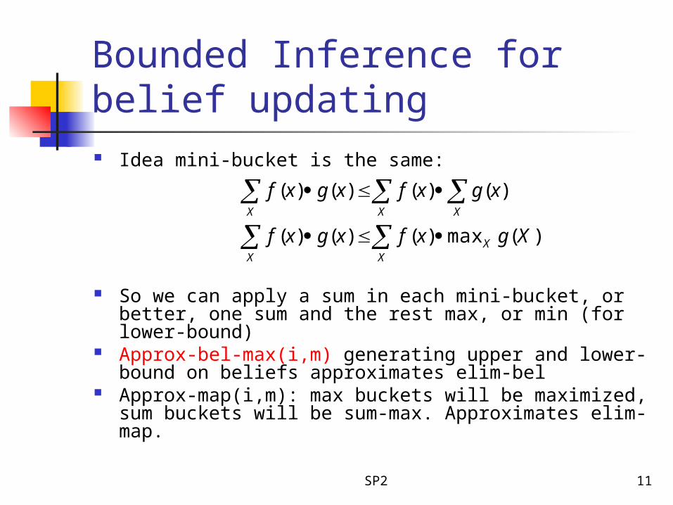
Bounded Inference for belief updating Idea mini-bucket is the same:

So we can apply a sum in each mini-bucket, or better, one sum and the rest max, or min (for lower-bound)

Approx-bel-max(i,m) generating upper and lower-bound on beliefs approximates elim-bel

Approx-map(i,m): max buckets will be maximized, sum buckets will be sum-max. Approximates elim-map.

)(max)()()(

)()()()(

Xgxfxgxf

xgxfxgxf

XX X

X X X

SP2 12

Empirical Evaluation(Dechter and Rish, 1997; Rish thesis, 1999)

Randomly generated networks Uniform random probabilities Random noisy-OR

CPCS networks Probabilistic decoding

Comparing approx-mpe and anytime-mpe

versus elim-mpe

SP2 13

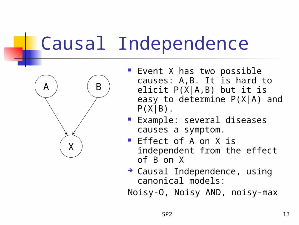
Causal Independence Event X has two possible

causes: A,B. It is hard to elicit P(X|A,B) but it is easy to determine P(X|A) and P(X|B).

Example: several diseases causes a symptom.

Effect of A on X is independent from the effect of B on X

Causal Independence, using canonical models:

Noisy-O, Noisy AND, noisy-max

A B

X

SP2 14

Binary ORA B

X

A B P(X=0|A,B)0 0 1

P(X=1|A,B)0

0 1 0 11 0 0 11 1 0 1

SP2 15

Noisy-OR“noise” is associated with each

edgedescribed by noise parameter

[0,1] :Let q b=0.2, qa =0.1

P(x=0|a,b)= (1-a) (1-b)

P(x=1|a,b)=1-(1-a) (1-b)

A B

X

A B P(X=0|A,B)0 0 1

P(X=1|A,B)0

a b

0 1 0.1 0.91 0 0.2 0.81 1 0.02 0.98

qi=P(X=0|A_i=1,…else =0)

SP2 16

Closed Form Bel(X) - 1

u

u

Tii

Tii

xifq

xifq

xP11

0

)u|(

Given: noisy-or CPT P(x|u)

noise parameters i

Tu = {i: Ui = 1}Define:

qi = 1 - I

Then:

SP2 17

Closed Form Bel(X) - 2Using Iterative Belief Propagation:

k

kxu i

i uqxxBEL )()()()u|(

u

u

Ti kkxi

u

Ti kkxi

u

xifuq

xifuq

xBEL1)()1(

0)(

)u|(1

0

Set piix = pix (uk=1). Then we can show that:

1)1(1

0)1(

)u|(1

0

xif

xif

xBEL

iixi

iixi

SP2 18

Methodology for Empirical Evakuation (for mpe) U/L –accuracy Better (U/mpe) or mpe/L Benchmarks: Random networks

Given n,e,v generate a random DAG For xi and parents generate table from

uniform [0,1], or noisy-or Create k instances. For each generate

random evidence, likely evidence Measure averages

SP2 19

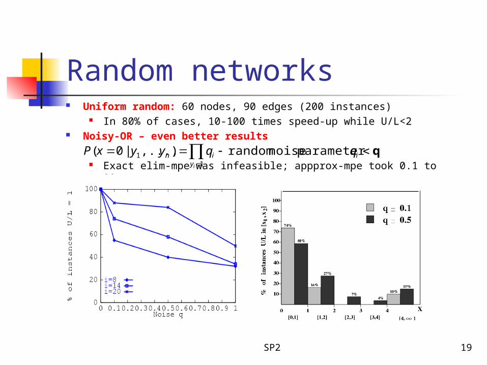
Random networks Uniform random: 60 nodes, 90 edges (200 instances)

In 80% of cases, 10-100 times speed-up while U/L<2 Noisy-OR – even better results

Exact elim-mpe was infeasible; appprox-mpe took 0.1 to 80 sec.

q

iy

in qqyyxPi

parameter noise random),...,|0(1

1

SP2 20

Anytime-mpe(0.0001) U/L error vs time

Time and parameter i

1 10 100 1000

Up

pe

r/L

ow

er

0.6

1.0

1.4

1.8

2.2

2.6

3.0

3.4

3.8 cpcs422b cpcs360b

i=1 i=21

CPCS networks – medical diagnosis(noisy-OR model)

Test case: no evidence

505.2 70.3anytime-mpe( ),

110.5 70.3anytime-mpe( ),

1697.6 115.8elim-mpe

cpcs422 cpcs360 AlgorithmTime (sec)

410 110

SP2 21

log(U/L)

0 2 4 6 8 10 12 0

100

200

300

400

500

600

700

800

900

1000

Freq

uenc

y

log(U/L) histogram for i=10 on 1000 instances of random evidence

log(U/L) histogram for i=10 on 1000 instances of likely evidence

log(U/L)

0 1 2 3 4 5 6 7 8 9 10 11 12 0

100

200

300

400

500

600

700

800

900

1000

Freq

uenc

y

The effect of evidence

More likely evidence=>higher MPE => higher accuracy (why?)

Likely evidence versus random (unlikely) evidence

SP2 22

Probabilistic decodingError-correcting linear block code

State-of-the-art: approximate algorithm – iterative belief propagation (IBP) (Pearl’s poly-tree algorithm applied to loopy networks)

SP2 23

Iterative Belief Proapagation

Belief propagation is exact for poly-trees IBP - applying BP iteratively to cyclic

networks

No guarantees for convergence Works well for many coding networks

)( 11uX

1U 2U 3U

2X1X

)( 12xU

)( 12uX

)( 13xU

) BEL(U update :step One

1

SP2 24

approx-mpe vs. IBPcodes *w-low onbetter is mpe-approx

codes w*)-(high generatedrandomly onbetter is IBP

Bit error rate (BER) as a function of noise (sigma):

SP2 25

Mini-buckets: summary Mini-buckets – local inference approximation

Idea: bound size of recorded functions

Approx-mpe(i) - mini-bucket algorithm for MPE Better results for noisy-OR than for random

problems Accuracy increases with decreasing noise in

coding Accuracy increases for likely evidence Sparser graphs -> higher accuracy Coding networks: approx-mpe outperfroms IBP on

low-induced width codes

SP2 26

Cluster Tree Elimination - properties Correctness and completeness: Algorithm CTE is

correct, i.e. it computes the exact joint probability of a single variable and the evidence.

Time complexity: O ( deg (n+N) d w*+1 )

Space complexity: O ( N d sep)where deg = the maximum degree of a node

n = number of variables (= number of CPTs)N = number of nodes in the tree

decompositiond = the maximum domain size of a variablew* = the induced widthsep = the separator size

SP2 27

Cluster Tree Elimination - the messages

),|()|()(),()2,1( bacpabpapcbha

A B C p(a), p(b|a), p(c|a,b)

B C D Fp(d|b), p(f|c,d)

h(1,2)(b,c)

B E Fp(e|b,f), h(2,3)(b,f)

E F Gp(g|e,f)

),(),|()|(),( )2,1(,

)3,2( cbhdcfpbdpfbhdc

2

4

1

3

EF

BC

BFsep(2,3)={B,F}

elim(2,3)={C,D}

SP2 28

Mini-Clustering for belief updating Motivation:

Time and space complexity of Cluster Tree Elimination depend on the induced width w* of the problem

When the induced width w* is big, CTE algorithm becomes infeasible

The basic idea: Try to reduce the size of the cluster (the exponent);

partition each cluster into mini-clusters with less variables Accuracy parameter i = maximum number of variables in a

mini-cluster The idea was explored for variable elimination (Mini-

Bucket)

SP2 29

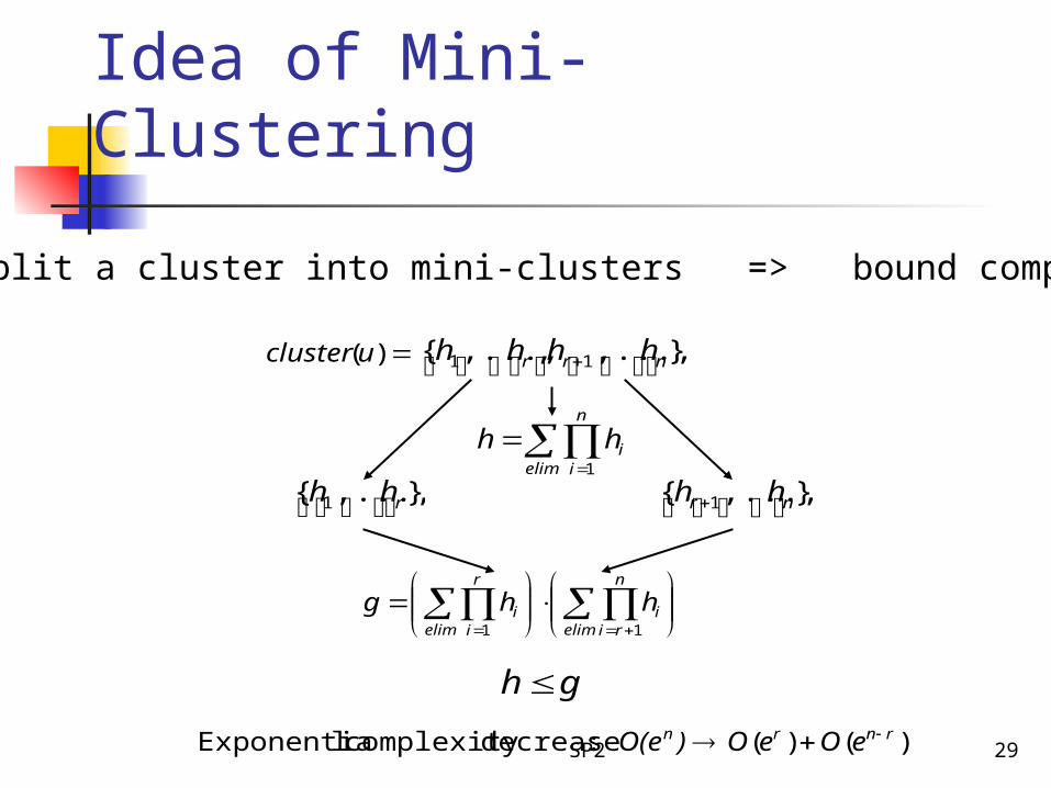
Idea of Mini-Clustering

Split a cluster into mini-clusters => bound complexity

)()( :decrease complexity lExponentia rnrn eOeO)O(e

},...,,,...,{ 11 nrr hhhh )(ucluster

elim

n

iihh

1

},...,{ 1 rhh },...,{ 1 nr hh

elim

n

rii

elim

r

ii hhg

11

gh

SP2 30

Mini-Clustering - MC

),|()|()(),(1)2,1( bacpabpapcbh

a


B E Fp(e|b,f)

E F Gp(g|e,f)

2

4

1

3

EF

BC

BF

dc

dcfpfh,

2)3,2( ),|()(

),()|()( 1)2,1(

,

1)3,2( cbhbdpbh

dc

dc

dcfpcbhbdpfbh,

1)2,1()3,2( ),|(),()|(),(

),|()|()(),()2,1( bacpabpapcbha

Cluster Tree Elimination Mini-Clustering, i=3

G

E

F

C D

B

A

B C D Fp(d|b), p(f|c,d)2

B C D Fp(d|b), h(1,2)(b,c), p(f|c,d)

sep(2,3) = {B,F}elim(2,3) = {C,D}

B C D C D FC D F p(d|b), h(1,2)(b,c) p(f|c,d)p(f|c,d)

SP2 31

Mini-Clustering - the messages, i=3

),|()|()(),(1)2,1( bacpabpapcbh

a


B C D p(d|b), h(1,2)(b,c)

C D F p(f|c,d)

B E Fp(e|b,f),

h1(2,3)(b), h2

(2,3)(f)

E F Gp(g|e,f)

2

4

1

3

EF

BC

BFsep(2,3)={B,F}

elim(2,3)={C,D} ),|(max)(,

2)3,2( dcfpfh

dc

),()|()( 1)2,1(

,

1)3,2( cbhbdpbh

dc

SP2 32

EF

BF

BC

),|()|()(:),(1)2,1( bacpabpapcbh

a

)2,1(H

),|(max:)(

),()|(:)(

,

2)1,2(

1)2,3(

,

1)1,2(

dcfpch

fbhbdpbh

fd

fd

)1,2(H

),|(max:)(

),()|(:)(

,

2)3,2(

1)2,1(

,

1)3,2(

dcfpfh

cbhbdpbh

dc

dc

)3,2(H

),(),|(:),( 1)3,4(

1)2,3( fehfbepfbh

e

)2,3(H

)()(),|(:),( 2)3,2(

1)3,2(

1)4,3( fhbhfbepfeh

b

)4,3(H

),|(:),(1)3,4( fegGpfeh e)3,4(H

ABC

2

4

1

3 BEF

EFG

BCDF

Mini-Clustering - example

SP2 34

Mini-Clustering

Correctness and completeness: Algorithm MC(i) computes a bound (or an approximation) on the joint probability P(Xi,e) of each variable and each of its values.

Time & space complexity: O(n hw* d i)

where hw* = maxu | {f | f (u) } |

SP2 35

We can replace max operator by

min => lower bound on the joint

mean => approximation of the joint

Lower bounds and mean approximations

SP2 36

MC can compute an (upper) bound on the joint P(Xi,e)

Deriving a bound on the conditional P(Xi|e) is not easy when the exact P(e) is not available

If a lower bound would be available, we could use:

as an upper bound on the posterior

In our experiments we normalized the results and regarded them as approximations of the posterior P(Xi|e)

),( eXP i

)(eP

)(/),( ePeXP i

Normalization

SP2 37

Experimental results

Algorithms: Exact IBP Gibbs sampling (GS) MC with normalization

(approximate)

Networks (all variables are binary):

Coding networks CPCS 54, 360, 422 Grid networks (MxM) Random noisy-OR networks Random networks

Measures: Normalized Hamming

Distance (NHD) BER (Bit Error Rate) Absolute error Relative error Time

SP2 38

Random networks - Absolute error

evidence=0 evidence=10

Random networks, N=50, P=2, k=2, evid=0, w*=10, 50 instances

i-bound

0 2 4 6 8 10

Abs

olut

e er

ror

0.00

0.02

0.04

0.06

0.08

0.10

0.12

0.14

0.16

MCGibbs SamplingIBP

Random networks, N=50, P=2, k=2, evid=10, w*=10, 50 instances

i-bound

0 2 4 6 8 10

Abs

olut

e er

ror

0.00

0.02

0.04

0.06

0.08

0.10

0.12

0.14

0.16

MCGibbs SamplingIBP

SP2 39

Noisy-OR networks - Absolute error

Noisy-OR networks, N=50, P=3, evid=10, w*=16, 25 instances

i-bound

0 2 4 6 8 10 12 14 16

Abs

olut

e er

ror

1e-5

1e-4

1e-3

1e-2

1e-1

1e+0

MCIBPGibbs Sampling

Noisy-OR networks, N=50, P=3, evid=20, w*=16, 25 instances

i-bound

0 2 4 6 8 10 12 14 16A

bsol

ute

erro

r1e-5

1e-4

1e-3

1e-2

1e-1

1e+0

MCIBPGibbs Sampling


SP2 40

Grid 15x15 - 10 evidenceGrid 15x15, evid=10, w*=22, 10 instances

i-bound

0 2 4 6 8 10 12 14 16 18

NH

D

0.00

0.02

0.04

0.06

0.08

0.10

0.12

0.14

MCIBP

Grid 15x15, evid=10, w*=22, 10 instances

i-bound

0 2 4 6 8 10 12 14 16 18

Abs

olut

e er

ror

0.00

0.01

0.02

0.03

0.04

0.05

0.06

MCIBP


i-bound

0 2 4 6 8 10 12 14 16 18

Rel

ativ

e er

ror

0.00

0.02

0.04

0.06

0.08

0.10

0.12

MCIBP


i-bound

0 2 4 6 8 10 12 14 16 18

Tim

e (

seco

nd

s)

0

2

4

6

8

10

12

MCIBP

SP2 41

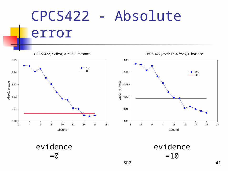
CPCS422 - Absolute error


CPCS 422, evid=0, w*=23, 1 instance

i-bound

2 4 6 8 10 12 14 16 18

Abs

olut

e er

ror

0.00

0.01

0.02

0.03

0.04

0.05

MCIBP

CPCS 422, evid=10, w*=23, 1 instance

i-bound

2 4 6 8 10 12 14 16 18

Abs

olut

e er

ror

0.00

0.01

0.02

0.03

0.04

0.05

MCIBP

SP2 42

Coding networks - Bit Error Rate

sigma=0.22 sigma=.51

Coding networks, N=100, P=4, sigma=.51, w*=12, 50 instances

i-bound

0 2 4 6 8 10 12

Bit

Err

or R

ate

0.06

0.08

0.10

0.12

0.14

0.16

0.18

MCIBP

Coding networks, N=100, P=4, sigma=.22, w*=12, 50 instances

i-bound

0 2 4 6 8 10 12

Bit

Err

or R

ate

0.000

0.001

0.002

0.003

0.004

0.005

0.006

0.007

MCIBP

SP2 43

Mini-Clustering summary

MC extends the partition based approximation from mini-buckets to general tree decompositions for the problem of belief updating

Empirical evaluation demonstrates its effectiveness and superiority (for certain types of problems, with respect to the measures considered) relative to other existing algorithms

SP2 44

What is IJGP?

IJGP is an approximate algorithm for belief updating in Bayesian networks

IJGP is a version of join-tree clustering which is both anytime and iterative

IJGP applies message passing along a join-graph, rather than a join-tree

Empirical evaluation shows that IJGP is almost always superior to other approximate schemes (IBP, MC)

SP2 45

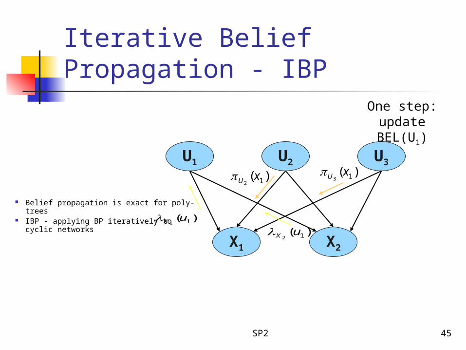
Iterative Belief Propagation - IBP

Belief propagation is exact for poly-trees IBP - applying BP iteratively to cyclic

networks

No guarantees for convergence

Works well for many coding networks

One step:update BEL(U1)

)( 11uX

U1

)( 12xU

)( 12uX

)( 13xU

U2 U3

X2X1

SP2 46

IJGP - Motivation IBP is applied to a loopy network iteratively

not an anytime algorithm when it converges, it converges very fast

MC applies bounded inference along a tree decomposition

MC is an anytime algorithm controlled by i-bound MC converges in two passes up and down the tree

IJGP combines: the iterative feature of IBP the anytime feature of MC

SP2 47

IJGP - The basic idea Apply Cluster Tree Elimination to any join-

graph

We commit to graphs that are minimal I-maps

Avoid cycles as long as I-mapness is not violated

Result: use minimal arc-labeled join-graphs

SP2 48

IJGP - ExampleA

D

I

B

E

J

F

G

C

H

A

ABDE

FGI

ABC

BCE

GHIJ

CDEF

FGH

C

H

A C

A AB BC

BE

C

CDE CE

FH

FFG GH H

GI

a) Belief network a) The graph IBP works on

SP2 49

Arc-minimal join-graphA

ABDE

FGI

ABC

BCE

GHIJ

CDEF

FGH

C

H

A C

A AB BC

BE

C

CDE CE

FH

FFG GH H

GI

A

ABDE

FGI

ABC

BCE

GHIJ

CDEF

FGH

C

H

A

AB BC

CDE CE

H

FFG GH

GI

SP2 50

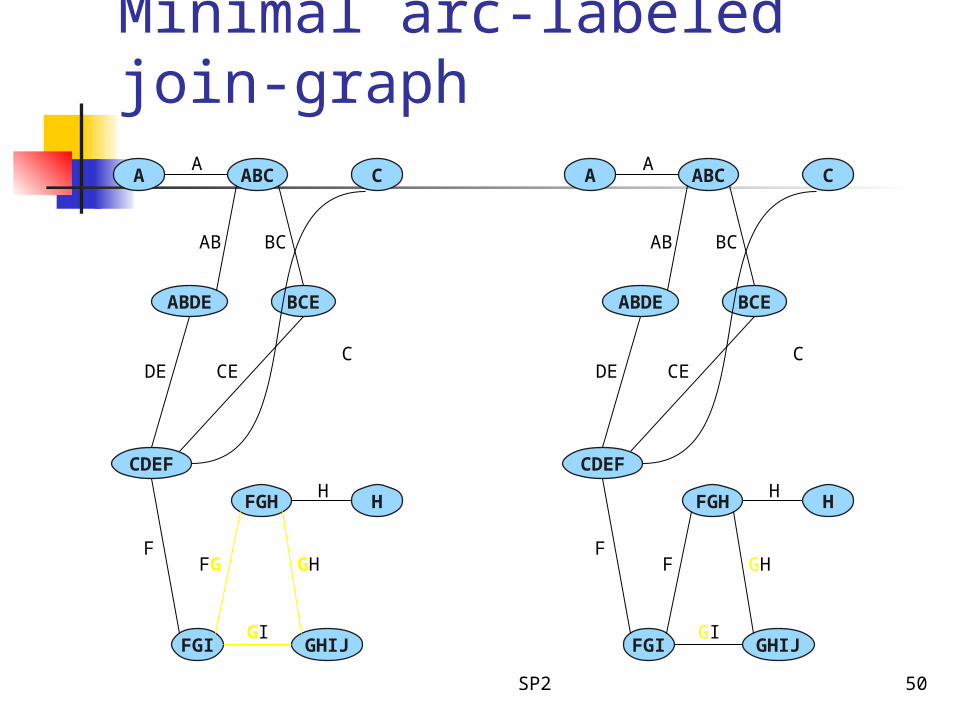
Minimal arc-labeled join-graph

A

ABDE

FGI

ABC

BCE

GHIJ

CDEF

FGH

C

H

A

AB BC

CDE CE

H

FFG GH

GI

A

ABDE

FGI

ABC

BCE

GHIJ

CDEF

FGH

C

H

A

AB BC

CDE CE

H

FF GH

GI

SP2 51

Join-graph decompositions

a) Minimal arc-labeled join graph

b) Join-graph obtained by collapsing nodes of graph a)

c) Minimal arc-labeled join graph

A

ABDE

FGI

ABC

BCE

GHIJ

CDEF

FGH

C

H

A

AB BC

CDE CE

H

FF GH

GI

ABCDE

FGI

BCE

GHIJ

CDEF

FGH

BC

CDE CE

FF GH

GI

ABCDE

FGI

BCE

GHIJ

CDEF

FGH

BC

DE CE

FF GH

GI

SP2 52

Tree decompositionABCDE

FGHI GHIJ

CDEF

CDE

F

GHI

a) Minimal arc-labeled join graph

a) Tree decomposition

ABCDE

FGI

BCE

GHIJ

CDEF

FGH

BC

DE CE

FF GH

GI

SP2 53

Join-graphsA

ABDE

FGI

ABC

BCE

GHIJ

CDEF

FGH

C

H

A C

A AB BC

BE

C

CDE CE

FH

FFG GH H

GI

A

ABDE

FGI

ABC

BCE

GHIJ

CDEF

FGH

C

H

A

AB BC

CDE CE

H

FF GH

GI

ABCDE

FGI

BCE

GHIJ

CDEF

FGH

BC

DE CE

FF GH

GI

ABCDE

FGHI GHIJ

CDEF

CDE

F

GHI

more accuracy

less complexity

SP2 54

Message propagationABCDE

FGI

BCE

GHIJ

CDEF

FGH

BC

CDE

CE

FF GH

GI

ABCDEp(a), p(c), p(b|ac), p(d|abe),p(e|b,c)

h(3,1)(bc)

BCD

CDEF

BC

CDE CE

1 3

2

h(3,1)(bc)

h(1,2)

Minimal arc-labeled: sep(1,2)={D,E} elim(1,2)={A,B,C}

Non-minimal arc-labeled: sep(1,2)={C,D,E} elim(1,2)={A,B}

cba

bchbcepabedpacbpcpapdeh,,

)1,3()2,1( )()|()|()|()()()(

ba

bchbcepabedpacbpcpapcdeh,

)1,3()2,1( )()|()|()|()()()(

SP2 55

Bounded decompositions We want arc-labeled decompositions such

that: the cluster size (internal width) is bounded by i (the

accuracy parameter) the width of the decomposition as a graph (external

width) is as small as possible

Possible approaches to build decompositions: partition-based algorithms - inspired by the mini-

bucket decomposition grouping-based algorithms

SP2 56

Partition-based algorithms

G

E

F

C D

B

A

a) schematic mini-bucket(i), i=3 b) arc-labeled join-graph decomposition

CDB

CAB

BA

A

CBP(D|B)

P(C|A,B)

P(A)

BA

P(B|A)

FCD

P(F|C,D)

GFE

EBF

BF

EFP(E|B,F)

P(G|F,E)

B

CD

BF

A

F

G: (GFE)

E: (EBF) (EF)

F: (FCD) (BF)

D: (DB) (CD)

C: (CAB) (CB)

B: (BA) (AB) (B)

A: (A)

SP2 57

IJGP properties IJGP(i) applies BP to min arc-labeled join-

graph, whose cluster size is bounded by i

On join-trees IJGP finds exact beliefs

IJGP is a Generalized Belief Propagation algorithm (Yedidia, Freeman, Weiss 2001)

Complexity of one iteration: time: O(deg•(n+N) •d i+1) space: O(N•d)

SP2 58

Empirical evaluation

Algorithms: Exact IBP MC IJGP

Measures: Absolute error Relative error Kulbach-Leibler (KL) distance Bit Error Rate Time

Networks (all variables are binary): Random networks Grid networks (MxM) CPCS 54, 360, 422 Coding networks

SP2 59

Random networks - KL at convergence

evidence=0

Random networks, N=50, K=2, P=3, evid=0, w*=16, 100 instances

i-bound1 2 3 4 5 6 7 8 9 10 11

KL

dist

ance

1e-5

1e-4

1e-3

1e-2

IJGPMCIBP


i-bound

1 2 3 4 5 6 7 8 9 10 11K

L di

stan

ce1e-5

1e-4

1e-3

1e-2

IJGPMCIBP

evidence=5

SP2 60

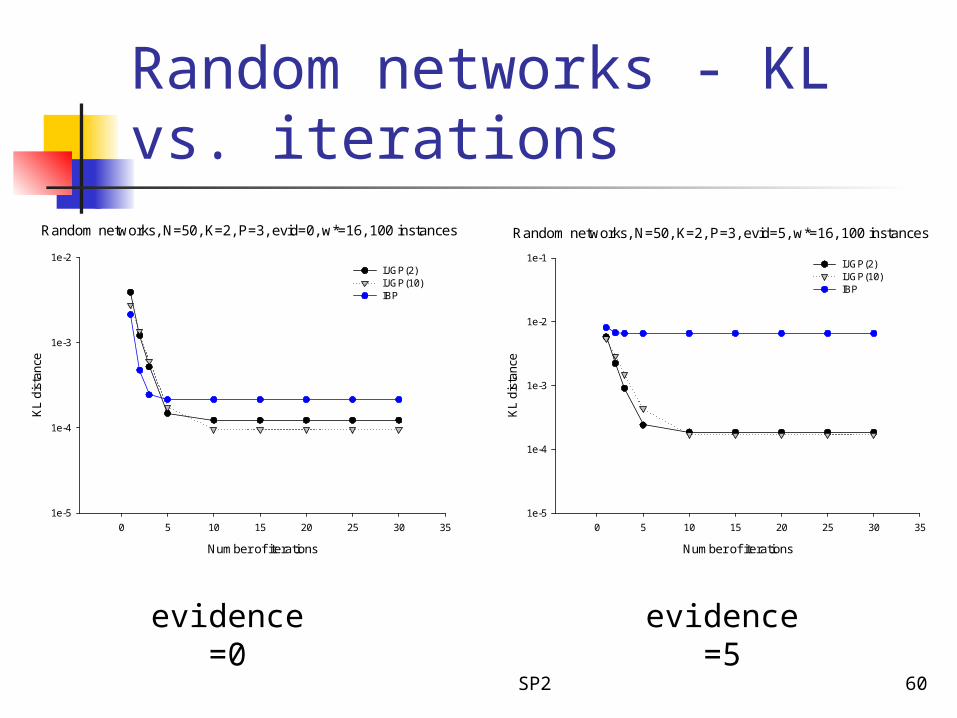
Random networks - KL vs. iterations



Number of iterations

0 5 10 15 20 25 30 35

KL

dist

ance

1e-5

1e-4

1e-3

1e-2IJGP(2)IJGP(10)IBP

Number of iterations

0 5 10 15 20 25 30 35

KL

dist

ance

1e-5

1e-4

1e-3

1e-2

1e-1IJGP(2)IJGP(10)IBP


SP2 61

Random networks - TimeRandom networks, N=50, K=2, P=3, evid=5, w*=16, 100 instances

i-bound

1 2 3 4 5 6 7 8 9 10 11

Tim

e (

seco

nds

)

0.0

0.2

0.4

0.6

0.8

1.0

IJGP 20 itMCIBP 10 it

SP2 62

Coding networks - BERCoding, N=400, 500 instances, 30 it, w*=43, sigma=.32

i-bound

0 2 4 6 8 10 12

BE

R

0.00237

0.00238

0.00239

0.00240

0.00241

0.00242

0.00243

IBPIJGP

Coding, N=400, 500 instances, 30 it, w*=43, sigma=.51

i-bound

0 2 4 6 8 10 12

BE

R

0.0745

0.0750

0.0755

0.0760

0.0765

0.0770

0.0775

0.0780

0.0785

IBPIJGP


i-bound

0 2 4 6 8 10 12

BE

R

0.1900

0.1902

0.1904

0.1906

0.1908

0.1910

0.1912

0.1914

IBPIJGP

sigma=.22 sigma=.32

sigma=.51 sigma=.65


i-bound

0 2 4 6 8 10 12

BE

R

1e-5

1e-4

1e-3

1e-2

1e-1

IJGPMCIBP

SP2 63

Coding networks - TimeCoding, N=400, 500 instances, 30 iterations, w*=43

i-bound

0 2 4 6 8 10 12

Tim

e (s

econ

ds)

0

2

4

6

8

10

IJGP 30 iterationsMCIBP 30 iterations

SP2 64

IJGP summary IJGP borrows the iterative feature from IBP and the

anytime virtues of bounded inference from MC

Empirical evaluation showed the potential of IJGP, which improves with iteration and most of the time with i-bound, and scales up to large networks

IJGP is almost always superior, often by a high margin, to IBP and MC

Based on all our experiments, we think that IJGP provides a practical breakthrough to the task of belief updating

SP2 65

Heuristic search Mini-buckets record upper-bound heuristics The evaluation function over

Best-first: expand a node with maximal evaluation function Branch and Bound: prune if f >= upper bound Properties:

an exact algorithm Better heuristics lead to more prunning

),...(x 1p pxx

pj buckethjp

p

iiip

ppp

hxh

paxPxg

xhxgxf

)(

)|()(

)()()(1

1

SP2 66

Heuristic Function

Given a cost functionP(a,b,c,d,e) = P(a) • P(b|a) • P(c|a) • P(e|b,c) • P(d|b,a)

Define an evaluation function over a partial assignment as theprobability of it’s best extension

f*(a,e,d) = maxb,c P(a,b,c,d,e) = = P(a) • maxb,c P)b|a) • P(c|a) • P(e|b,c) • P(d|a,b)

= g(a,e,d) • H*(a,e,d)

E

E

DA

D

B

D

D

B0

1

1

0

1

0

SP2 67

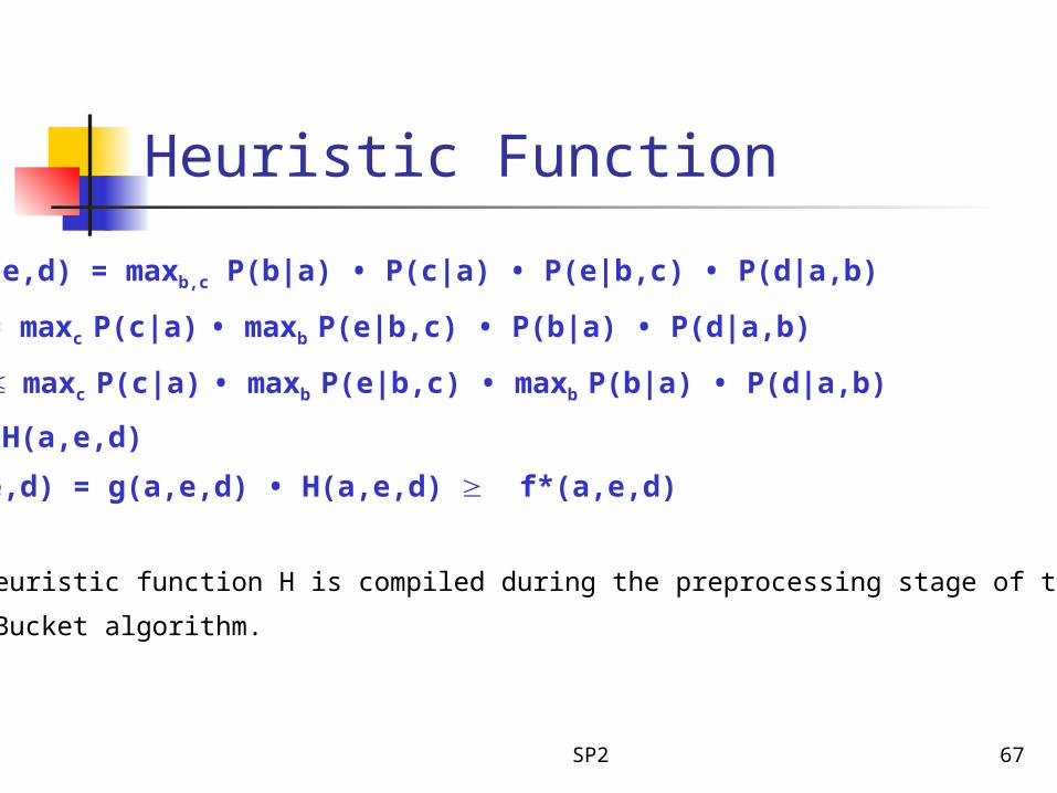
Heuristic Function

H*(a,e,d) = maxb,c P(b|a) • P(c|a) • P(e|b,c) • P(d|a,b)

= maxc P(c|a) • maxb P(e|b,c) • P(b|a) • P(d|a,b)

maxc P(c|a) • maxb P(e|b,c) • maxb P(b|a) • P(d|a,b)

= H(a,e,d)

f(a,e,d) = g(a,e,d) • H(a,e,d) f*(a,e,d)

The heuristic function H is compiled during the preprocessing stage of the

Mini-Bucket algorithm.

SP2 68

maxB P(e|b,c) P(d|a,b) P(b|a)

maxC P(c|a) hB(e,c)

maxD hB(d,a)

maxE hC(e,a)

maxA P(a) hE(a) hD (a)

Heuristic Function

The evaluation function f(xp) can be computed using function

recorded by the Mini-Bucket scheme and can be used to estimate

the probability of the best extension of partial assignment xp={x1, …, xp},

f(xp)=g(xp) H(xp )

For example,

H(a,e,d) = hB(d,a) hC (e,a)

g(a,e,d) = P(a)

SP2 69

Properties

Heuristic is monotone Heuristic is admissible Heuristic is computed in linear time IMPORTANT:

Mini-buckets generate heuristics of varying strength using control parameter – bound I

Higher bound -> more preprocessing -> stronger heuristics -> less search Allows controlled trade-off between

preprocessing and search

SP2 70

Empirical Evaluation of mini-bucket heuristics

Time [sec]

0 10 20 30

% S

olve

d E

xact

ly

0.0

0.1

0.2

0.3

0.4

0.5

0.6

0.7

0.8

0.9

1.0

BBMB i=2

BFMB i=2

BBMB i=6

BFMB i=6

BBMB i=10

BFMB i=10

BBMB i=14

BFMB i=14

Random Coding, K=100, noise 0.32

Time [sec]

0 10 20 30

% S

olve

d E

xact

ly

0.0

0.1

0.2

0.3

0.4

0.5

0.6

0.7

0.8

0.9

1.0

BBMB i=6 BFMB i=6 BBMB i=10 BFMB i=10 BBMB i=14 BFMB i=14

Documents

Approximation Techniques bounded inference COMPSCI 276 Fall 2007