Embed Size (px)
Citation preview
Approximation Techniques Iterative bounded inference
COMPSCI 276, Fall 2014
Set 11: Rina Dechter
(Reading: class notes chapter 8,9, Darwiche chapters 14)
Agenda
Mini-bucket elimination
Mini-clustering
Iterative Belief propagation
Iterative-join-graph propagation
IJGP complexity
Convergence and pair-wise consistency
Accuracy when converged
Belief Propagation and constraint propagation
Using Mini-bucket as heuristics for optimization
2
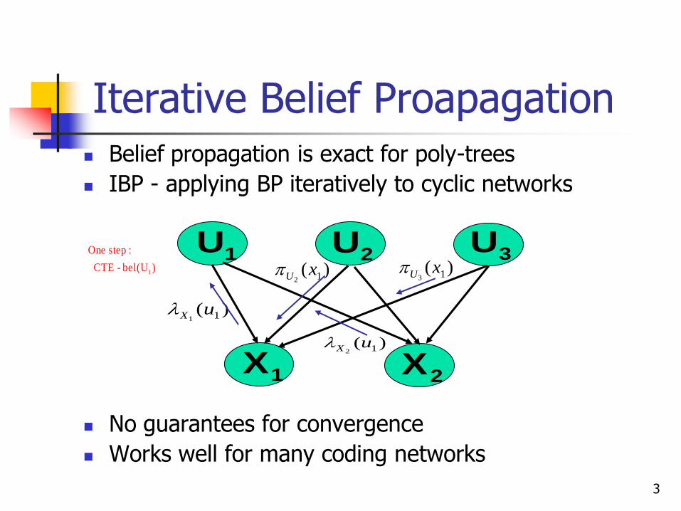
Iterative Belief Proapagation Belief propagation is exact for poly-trees
IBP - applying BP iteratively to cyclic networks
No guarantees for convergence
Works well for many coding networks
3
)( 11uX
1U 2U 3U
2X1X
)( 12xU
)( 12uX
)( 13xU)bel(U-CTE
:step One
1
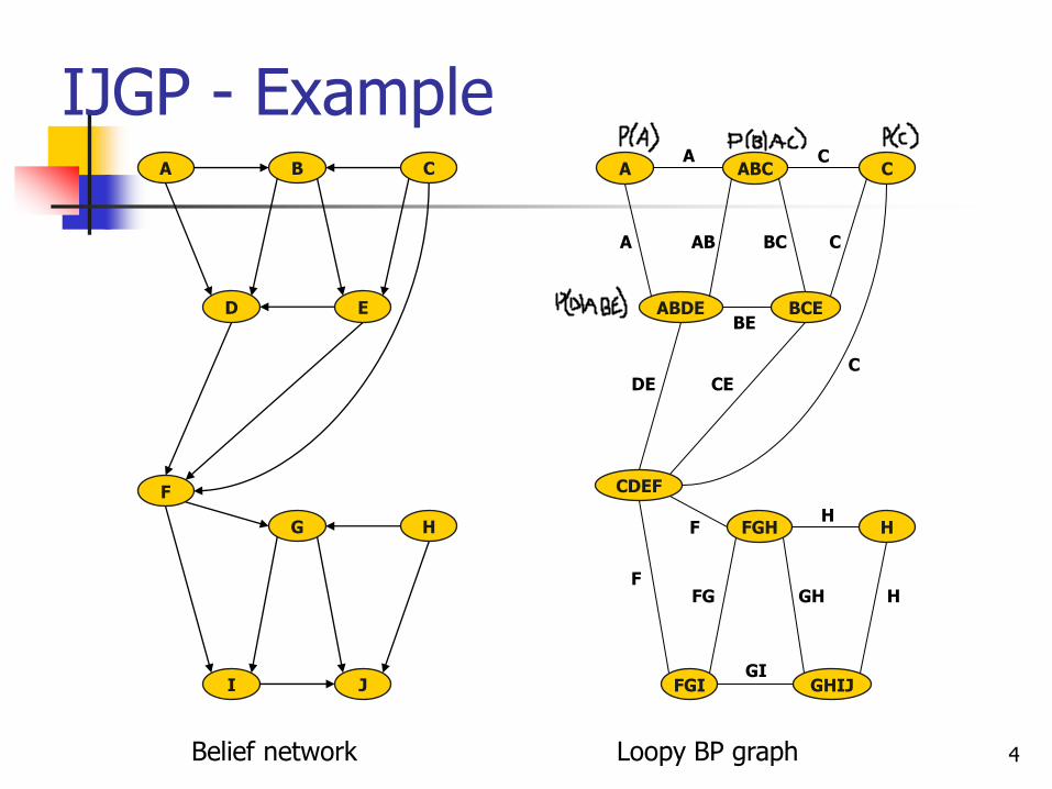
IJGP - Example
4
A
D
I
B
E
J
F
G
C
H
Belief network
A
ABDE
FGI
ABC
BCE
GHIJ
CDEF
FGH
C
H
A C
A AB BC
BE
C
C DE CE
F H
F FG GH H
GI
Loopy BP graph
5
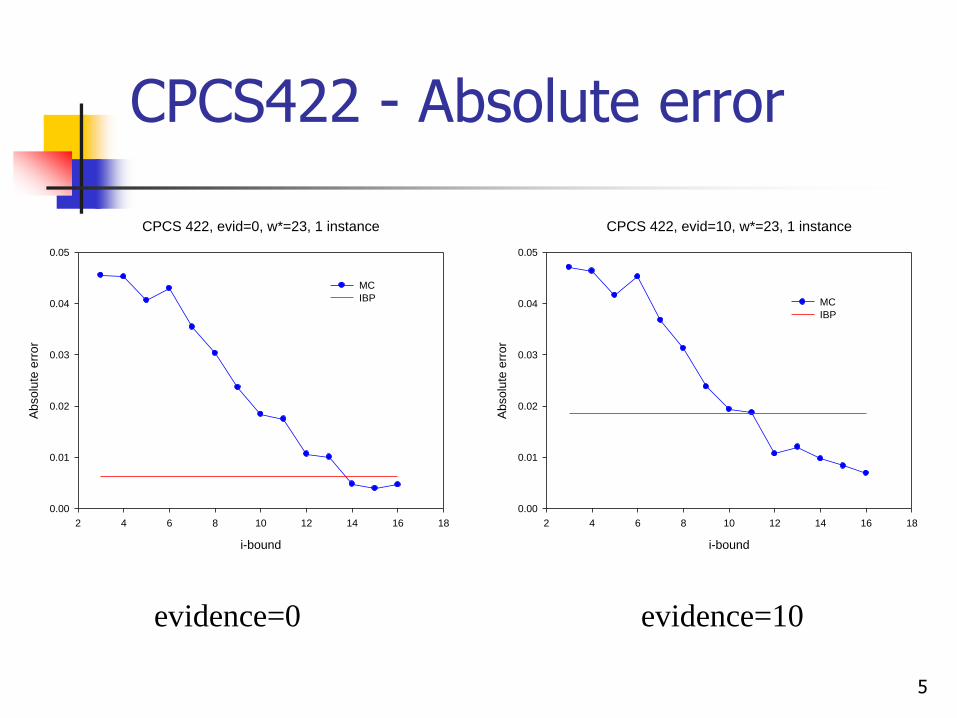
CPCS422 - Absolute error
evidence=0 evidence=10
CPCS 422, evid=0, w*=23, 1 instance
i-bound
2 4 6 8 10 12 14 16 18
Absolu
te e
rror
0.00
0.01
0.02
0.03
0.04
0.05
MC
IBP
CPCS 422, evid=10, w*=23, 1 instance
i-bound
2 4 6 8 10 12 14 16 18
Absolu
te e
rror
0.00
0.01
0.02
0.03
0.04
0.05
MC
IBP
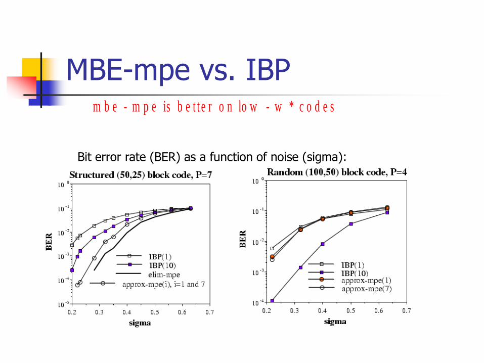
MBE-mpe vs. IBP
6
c o d e s *w-lo w o nb e t t e r is m p e-m b e
Bit error rate (BER) as a function of noise (sigma):

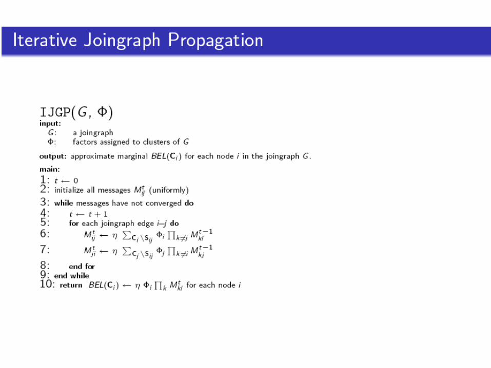
Iterative Join Graph Propagation
Loopy Belief Propagation Cyclic graphs Iterative Converges fast in practice (no guarantees though) Very good approximations (e.g., turbo decoding, LDPC codes, SAT
– survey propagation)
Mini-Clustering(i) Tree decompositions Only two sets of messages (inward, outward) Anytime behavior – can improve with more time by increasing the
i-bound
We want to combine:
Iterative virtues of Loopy BP Anytime behavior of Mini-Clustering(i)
7
IJGP - The basic idea
Apply Cluster Tree Elimination to any join-graph
We commit to graphs that are I-maps
Avoid cycles as long as I-mapness is not violated
Result: use minimal arc-labeled join-graphs
8
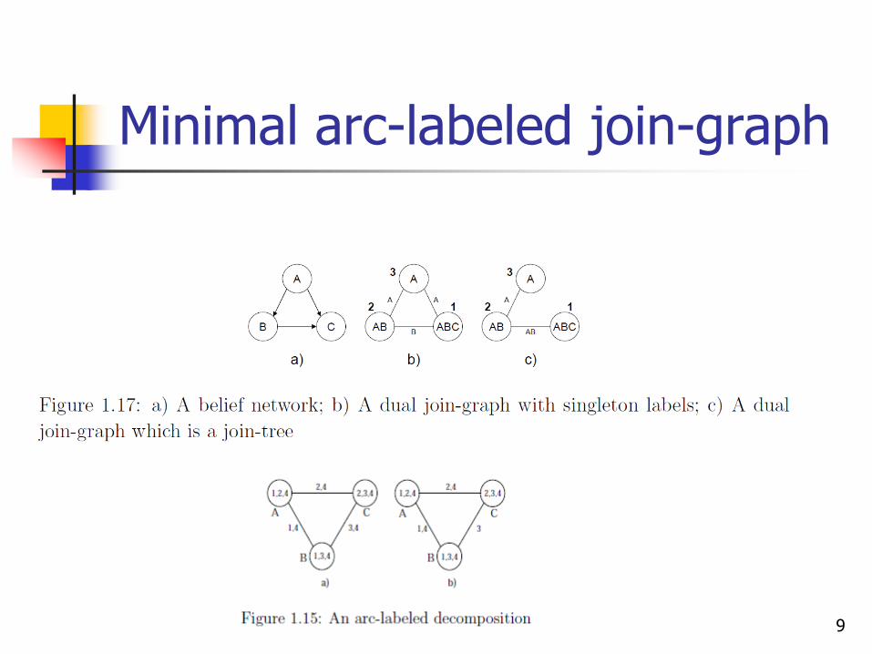
Minimal arc-labeled join-graph
9

IJGP - Example
10
A
D
I
B
E
J
F
G
C
H
Belief network
A
ABDE
FGI
ABC
BCE
GHIJ
CDEF
FGH
C
H
A C
A AB BC
BE
C
C DE CE
F H
F FG GH H
GI
Loopy BP graph
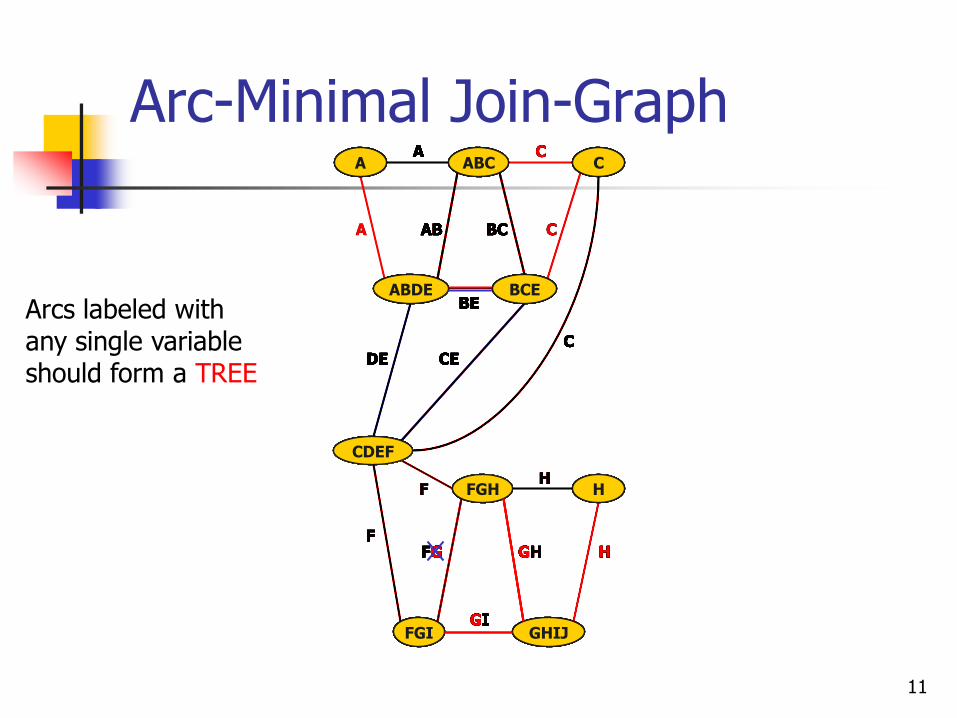
Arc-Minimal Join-Graph
11
A
ABDE
FGI
ABC
BCE
GHIJ
CDEF
FGH
C
H
A C
A AB BC
BE
C
C DE CE
F H
F FG GH H
GI
A
ABDE
FGI
ABC
BCE
GHIJ
CDEF
FGH
C
H
A C
A AB BC
BE
C
C DE CE
F H
F FG GH H
GI
A
ABDE
FGI
ABC
BCE
GHIJ
CDEF
FGH
C
H
A C
AB BC
BE
C
C DE CE
F H
F FG GH H
GI
A
ABDE
FGI
ABC
BCE
GHIJ
CDEF
FGH
C
H
A C
AB BC
BE
C
C DE CE
F H
F FG GH H
GI
A
ABDE
FGI
ABC
BCE
GHIJ
CDEF
FGH
C
H
A
AB BC
BE
C DE CE
F H
F FG GH H
GI
A
ABDE
FGI
ABC
BCE
GHIJ
CDEF
FGH
C
H
A
AB BC
BE
C DE CE
F H
F FG GH H
GI
A
ABDE
FGI
ABC
BCE
GHIJ
CDEF
FGH
C
H
A
AB BC
BE
C DE CE
F H
F FG GH H
GI
A
ABDE
FGI
ABC
BCE
GHIJ
CDEF
FGH
C
H
A
AB BC
C DE CE
F H
F FG GH H
GI
A
ABDE
FGI
ABC
BCE
GHIJ
CDEF
FGH
C
H
A
AB BC
BE
C DE CE
H
F FG GH H
GI
A
ABDE
FGI
ABC
BCE
GHIJ
CDEF
FGH
C
H
A
AB BC
BE
C DE CE
H
F FG GH H
GI
A
ABDE
FGI
ABC
BCE
GHIJ
CDEF
FGH
C
H
A
AB BC
BE
C DE CE
H
F FG GH
GI
A
ABDE
FGI
ABC
BCE
GHIJ
CDEF
FGH
C
H
A
AB BC
BE
C DE CE
H
F FG GH
GI
A
ABDE
FGI
ABC
BCE
GHIJ
CDEF
FGH
C
H
A
AB BC
BE
C DE CE
H
F FG GH
GI
Arcs labeled with any single variable should form a TREE
A
ABDE
FGI
ABC
BCE
GHIJ
CDEF
FGH
C
H
A
AB BC
BE
C DE CE
H
F FG GH
GI
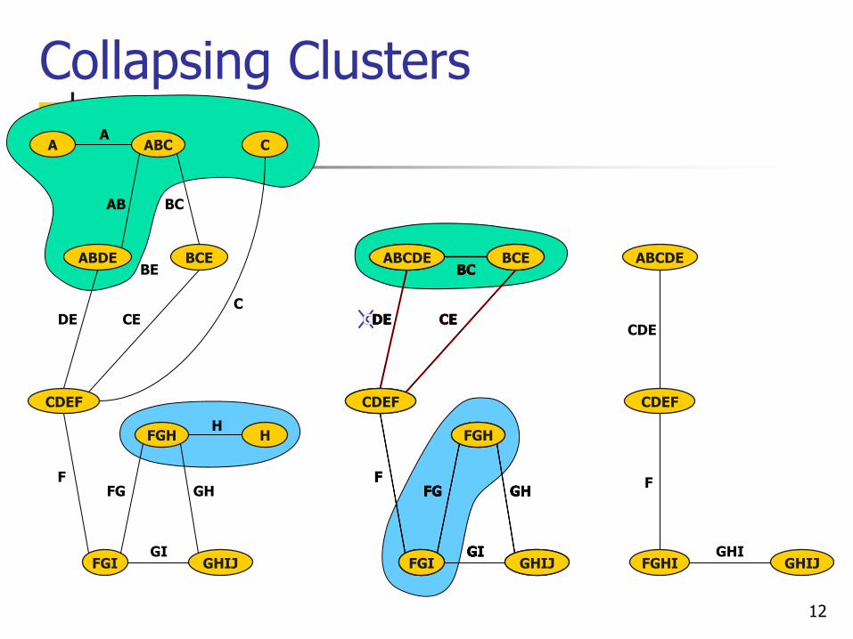
Collapsing Clusters
12
ABCDE
FGI
BCE
GHIJ
CDEF
FGH
BC
CDE CE
F FG GH
GI
ABCDE
FGI
BCE
GHIJ
CDEF
FGH
BC
CDE CE
F FG GH
GI
ABCDE
FGI
BCE
GHIJ
CDEF
FGH
BC
CDE CE
F FG GH
GI
ABCDE
FGHI GHIJ
CDEF
CDE
F
GHI
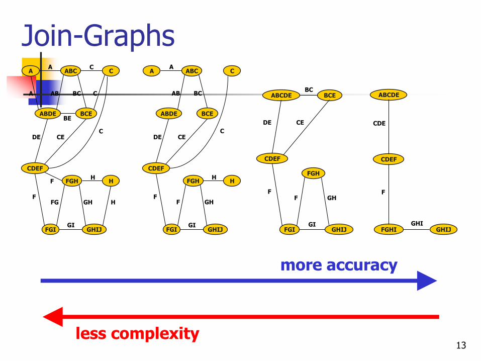
Join-Graphs
13
A
ABDE
FGI
ABC
BCE
GHIJ
CDEF
FGH
C
H
A C
A AB BC
BE
C
C DE CE
F H
F FG GH H
GI
A
ABDE
FGI
ABC
BCE
GHIJ
CDEF
FGH
C
H
A
AB BC
C DE CE
H
F F GH
GI
ABCDE
FGI
BCE
GHIJ
CDEF
FGH
BC
DE CE
F F GH
GI
ABCDE
FGHI GHIJ
CDEF
CDE
F
GHI
more accuracy
less complexity
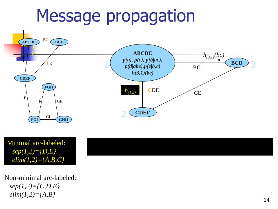
Message propagation
14
ABCDE
FGI
BCE
GHIJ
CDEF
FGH
BC
CDE
CE
F F GH
GI
ABCDE
p(a), p(c), p(b|ac),
p(d|abe),p(e|b,c)
h(3,1)(bc)
BCD
CDEF
BC
CDE CE
1 3
2
h(3,1)(bc)
h(1,2)
Minimal arc-labeled:
sep(1,2)={D,E}
elim(1,2)={A,B,C}
Non-minimal arc-labeled:
sep(1,2)={C,D,E}
elim(1,2)={A,B}
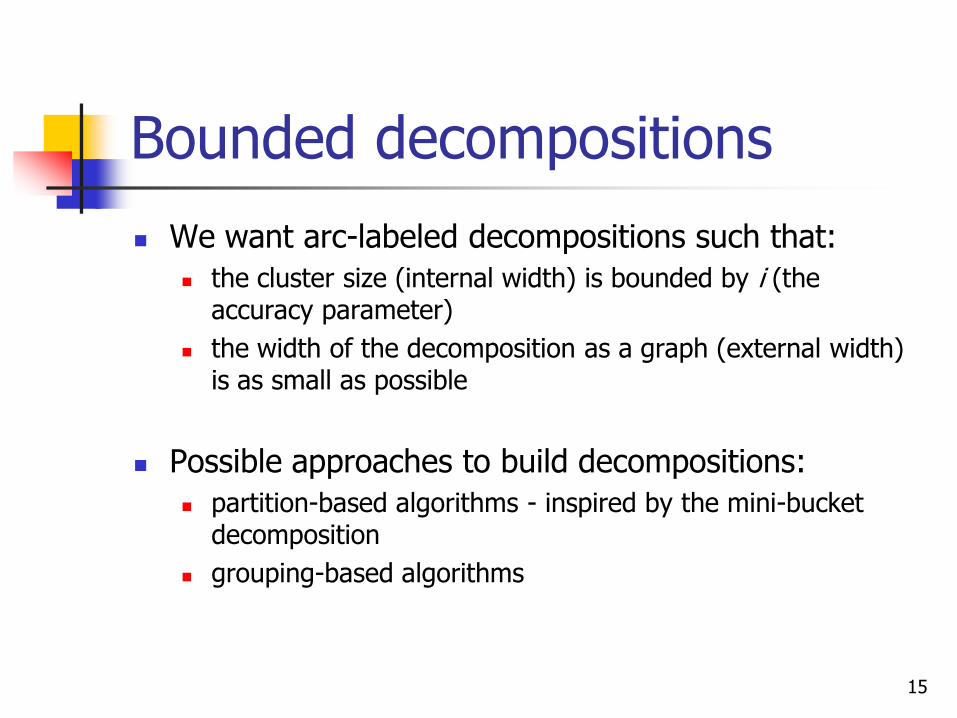
Bounded decompositions
We want arc-labeled decompositions such that:
the cluster size (internal width) is bounded by i (the accuracy parameter)
the width of the decomposition as a graph (external width) is as small as possible
Possible approaches to build decompositions:
partition-based algorithms - inspired by the mini-bucket decomposition
grouping-based algorithms
15
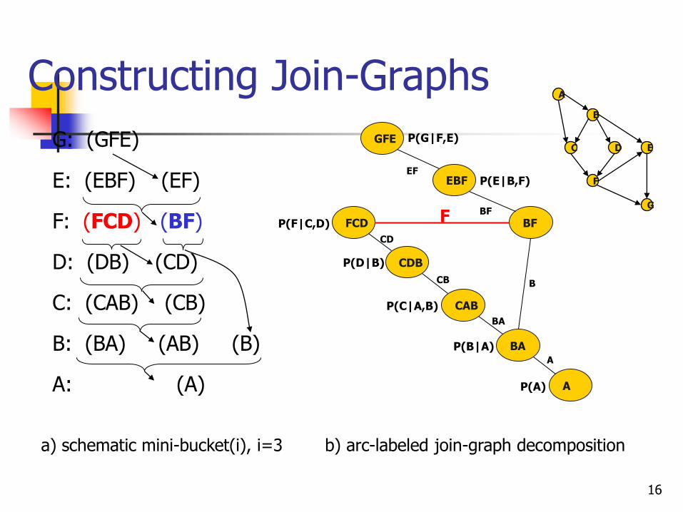
Constructing Join-Graphs
16
a) schematic mini-bucket(i), i=3 b) arc-labeled join-graph decomposition
CDB
CAB
BA
A
CB
P(D|B)
P(C|A,B)
P(A)
BA
P(B|A)
FCD P(F|C,D)
GFE
EBF
BF
EF P(E|B,F)
P(G|F,E)
B
CD
BF
A
F
G: (GFE)
E: (EBF) (EF)
F: (FCD) (BF)
D: (DB) (CD)
C: (CAB) (CB)
B: (BA) (AB) (B)
A: (A)
G
E
F
C D
B
A
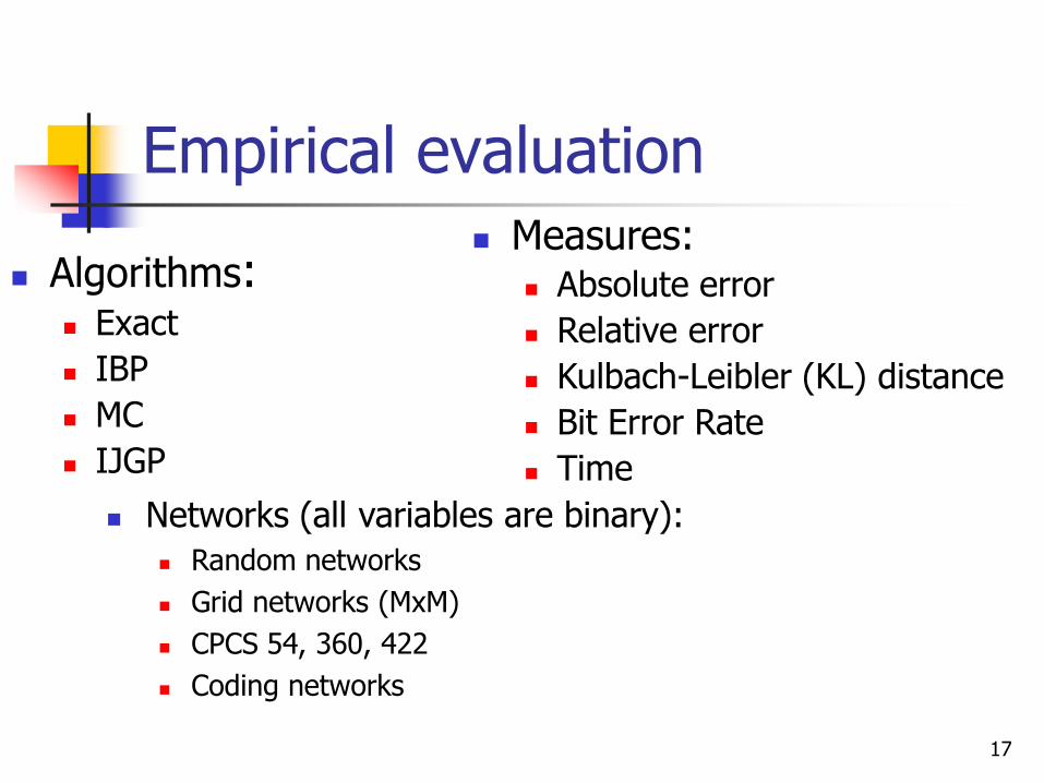
Empirical evaluation
17
Algorithms: Exact
IBP
MC
IJGP
Measures: Absolute error
Relative error
Kulbach-Leibler (KL) distance
Bit Error Rate
Time
Networks (all variables are binary):
Random networks
Grid networks (MxM)
CPCS 54, 360, 422
Coding networks
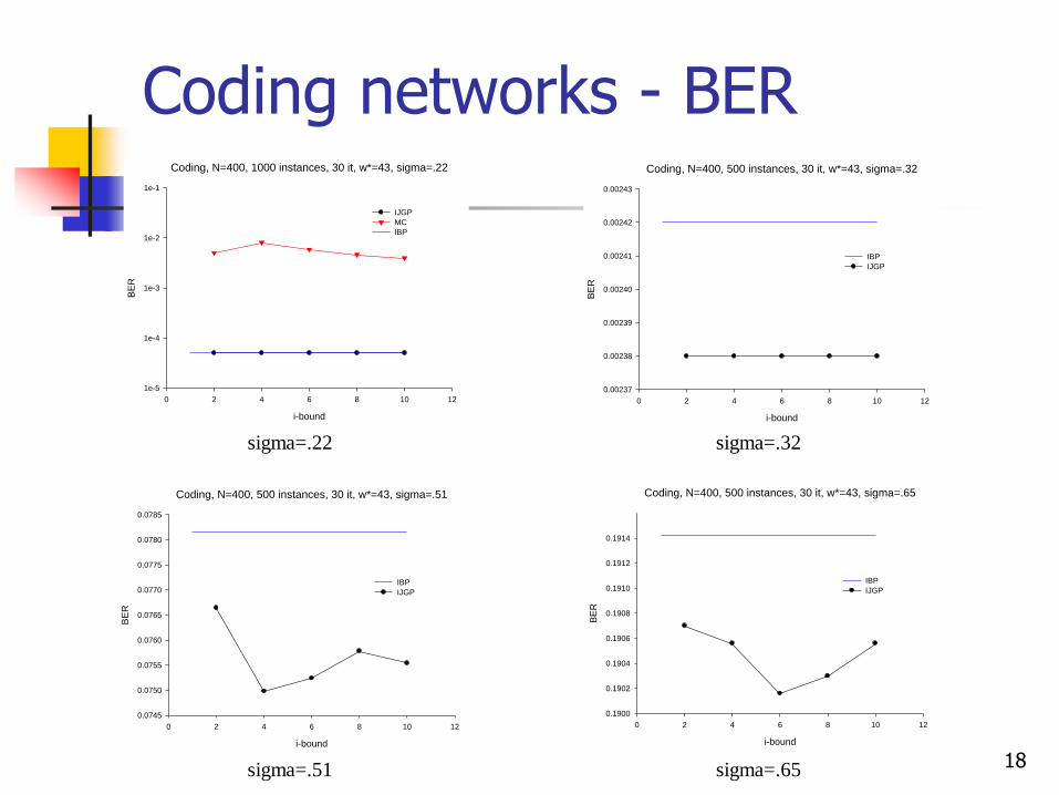
Coding networks - BER
18
Coding, N=400, 500 instances, 30 it, w*=43, sigma=.32
i-bound
0 2 4 6 8 10 12
BE
R
0.00237
0.00238
0.00239
0.00240
0.00241
0.00242
0.00243
IBP
IJGP
Coding, N=400, 500 instances, 30 it, w*=43, sigma=.51
i-bound
0 2 4 6 8 10 12
BE
R
0.0745
0.0750
0.0755
0.0760
0.0765
0.0770
0.0775
0.0780
0.0785
IBP
IJGP
Coding, N=400, 500 instances, 30 it, w*=43, sigma=.65
i-bound
0 2 4 6 8 10 12
BE
R
0.1900
0.1902
0.1904
0.1906
0.1908
0.1910
0.1912
0.1914
IBP
IJGP
sigma=.22 sigma=.32
sigma=.51 sigma=.65
Coding, N=400, 1000 instances, 30 it, w*=43, sigma=.22
i-bound
0 2 4 6 8 10 12
BE
R
1e-5
1e-4
1e-3
1e-2
1e-1
IJGP
MC
IBP
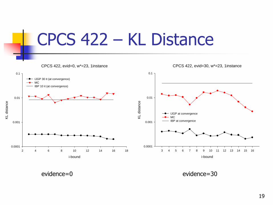
CPCS 422, evid=0, w*=23, 1instance
i-bound
2 4 6 8 10 12 14 16 18
KL
dis
tan
ce
0.0001
0.001
0.01
0.1
IJGP 30 it (at convergence)
MC
IBP 10 it (at convergence)
CPCS 422 – KL Distance
19
CPCS 422, evid=30, w*=23, 1instance
i-bound
3 4 5 6 7 8 9 10 11 12 13 14 15 16
KL
dis
tan
ce
0.0001
0.001
0.01
0.1
IJGP at convergence
MC
IBP at convergence
evidence=0 evidence=30
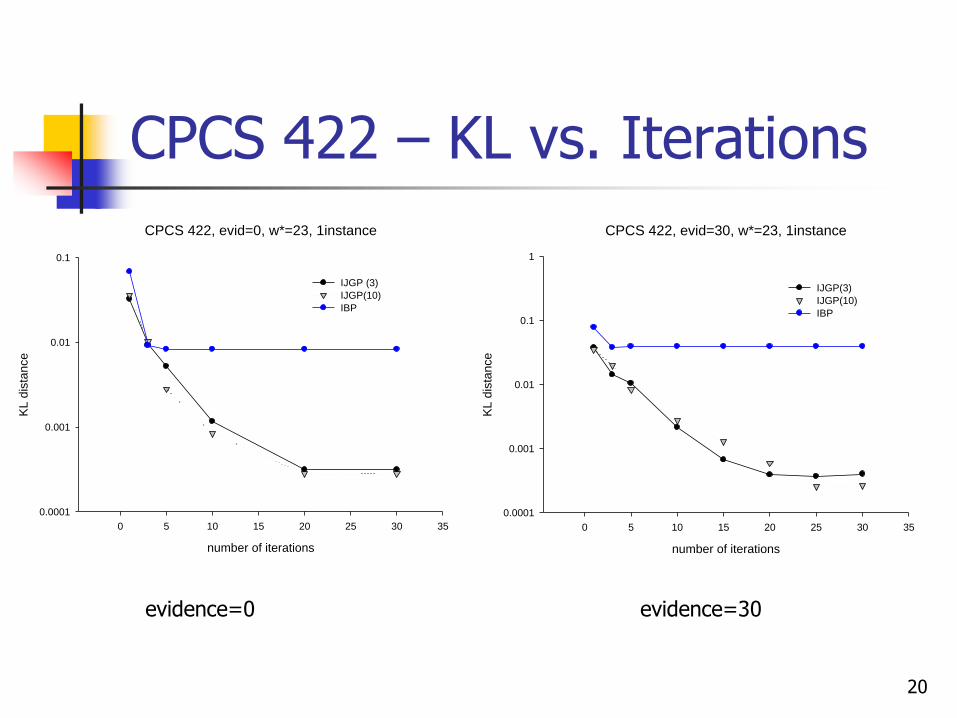
CPCS 422 – KL vs. Iterations
20
CPCS 422, evid=0, w*=23, 1instance
number of iterations
0 5 10 15 20 25 30 35
KL
dis
tan
ce
0.0001
0.001
0.01
0.1
IJGP (3)
IJGP(10)
IBP
CPCS 422, evid=30, w*=23, 1instance
number of iterations
0 5 10 15 20 25 30 35
KL d
ista
nce
0.0001
0.001
0.01
0.1
1
IJGP(3)
IJGP(10)
IBP
evidence=0 evidence=30
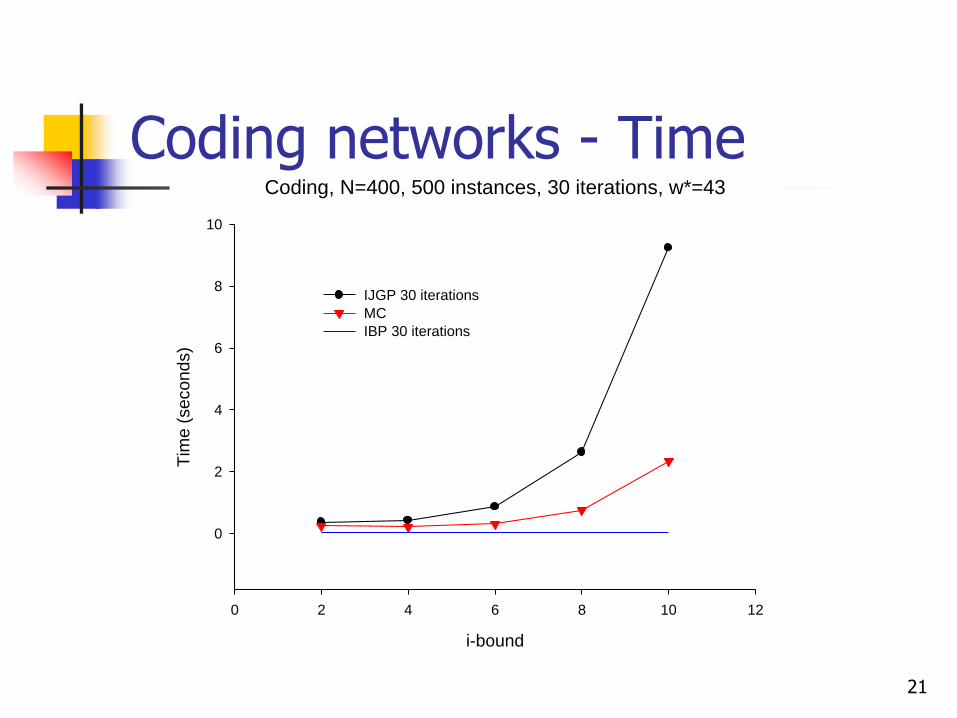
Coding networks - Time
21
Coding, N=400, 500 instances, 30 iterations, w*=43
i-bound
0 2 4 6 8 10 12
Tim
e (
se
co
nd
s)
0
2
4
6
8
10
IJGP 30 iterations
MC
IBP 30 iterations
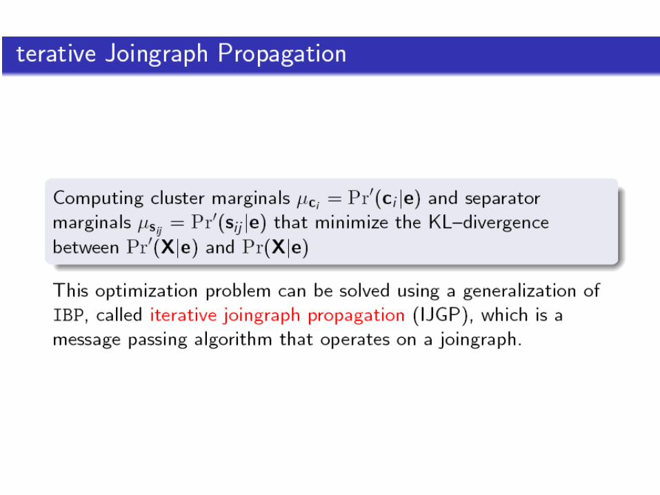
IJGP properties
IJGP(i) applies BP to min arc-labeled join-graph, whose cluster size is bounded by i
On join-trees IJGP finds exact beliefs
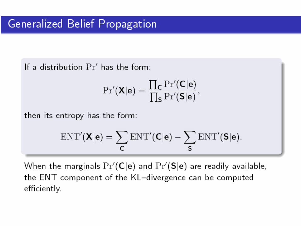
IJGP is a Generalized Belief Propagation algorithm (Yedidia, Freeman, Weiss 2001)
Complexity of one iteration:
time: O(deg•(n+N) •d i+1)
space: O(N•d)
22
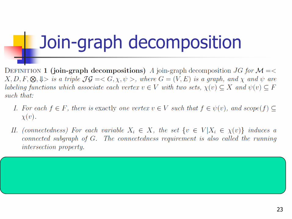
Join-graph decomposition
23
Agenda
Mini-bucket elimination
Mini-clustering
Iterative Belief propagation
Iterative-join-graph propagation
IJGP complexity
Convergence and pair-wise consistency
Accuracy when converged
BP and constraint propagation
24
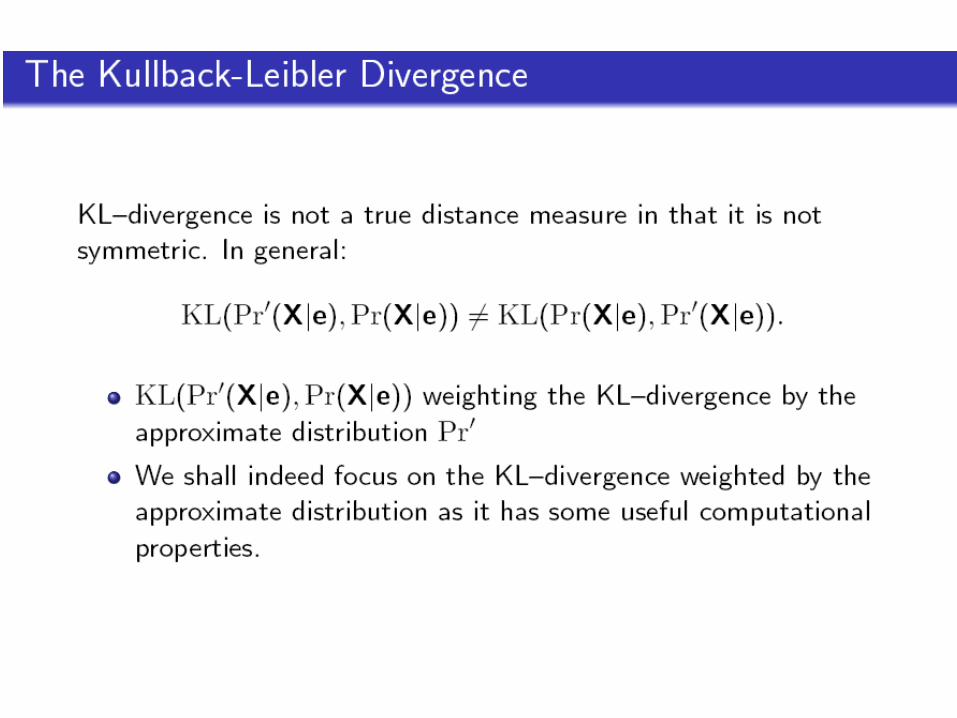
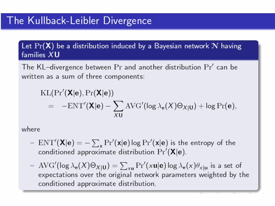
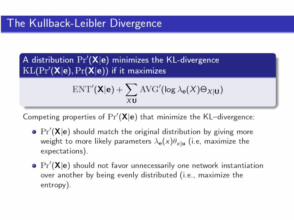
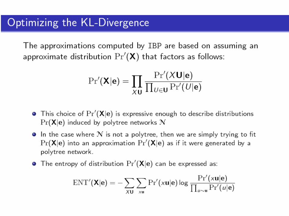
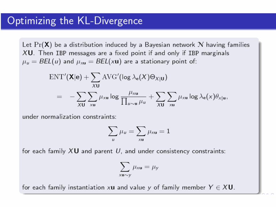
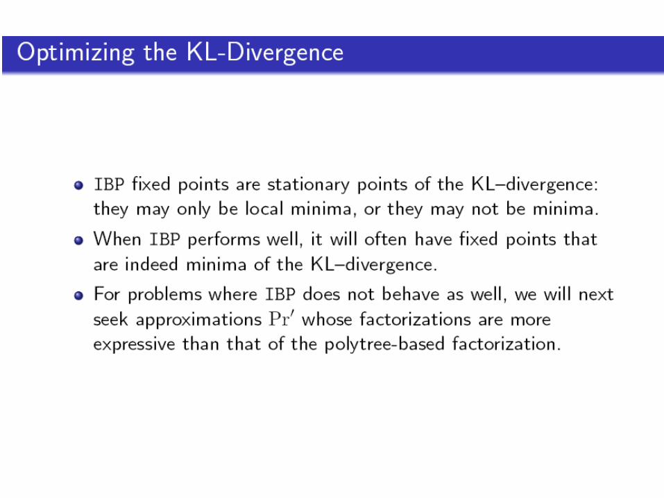
More On the Power of Belief Propagation
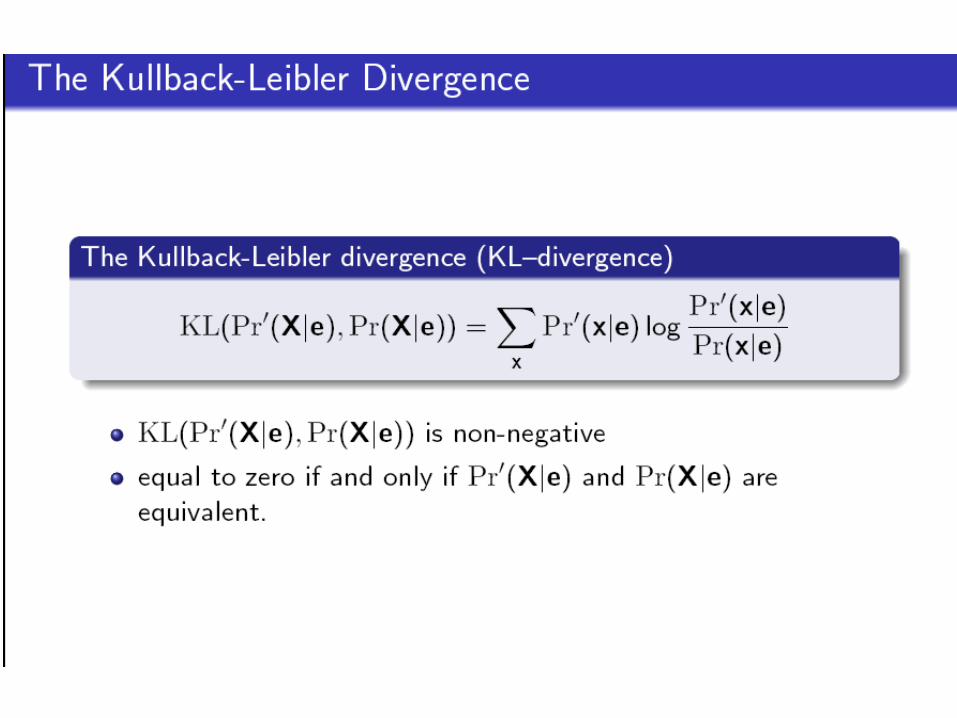
BP as local minima of KL distance
BP’s power from constraint propagation perspective.
25
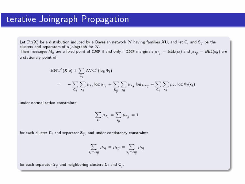
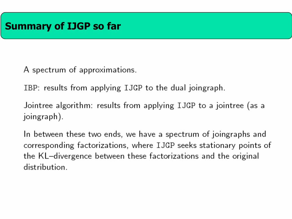
Summary of IJGP so far
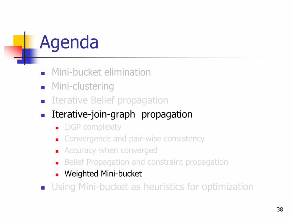
Agenda
Mini-bucket elimination
Mini-clustering
Iterative Belief propagation
Iterative-join-graph propagation
IJGP complexity
Convergence and pair-wise consistency
Accuracy when converged
Belief Propagation and constraint propagation
Weighted Mini-bucket
Using Mini-bucket as heuristics for optimization
38
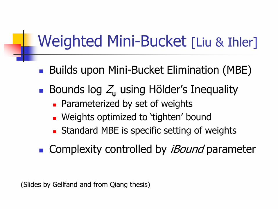
Weighted Mini-Bucket [Liu & Ihler]
Builds upon Mini-Bucket Elimination (MBE)
Bounds log Zψ using Hölder’s Inequality
Parameterized by set of weights
Weights optimized to ‘tighten’ bound
Standard MBE is specific setting of weights
Complexity controlled by iBound parameter
(Slides by Gellfand and from Qiang thesis)
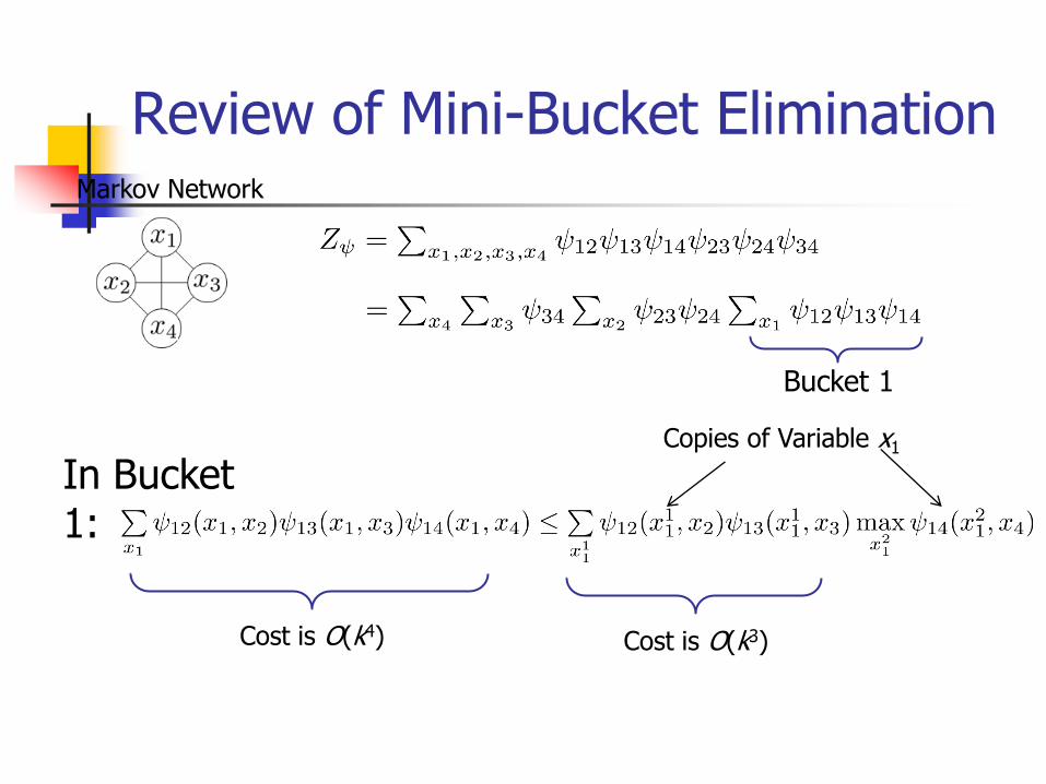
Review of Mini-Bucket Elimination Markov Network
Cost is O(k4)
In Bucket 1:
Cost is O(k3)
Copies of Variable x1
Bucket 1
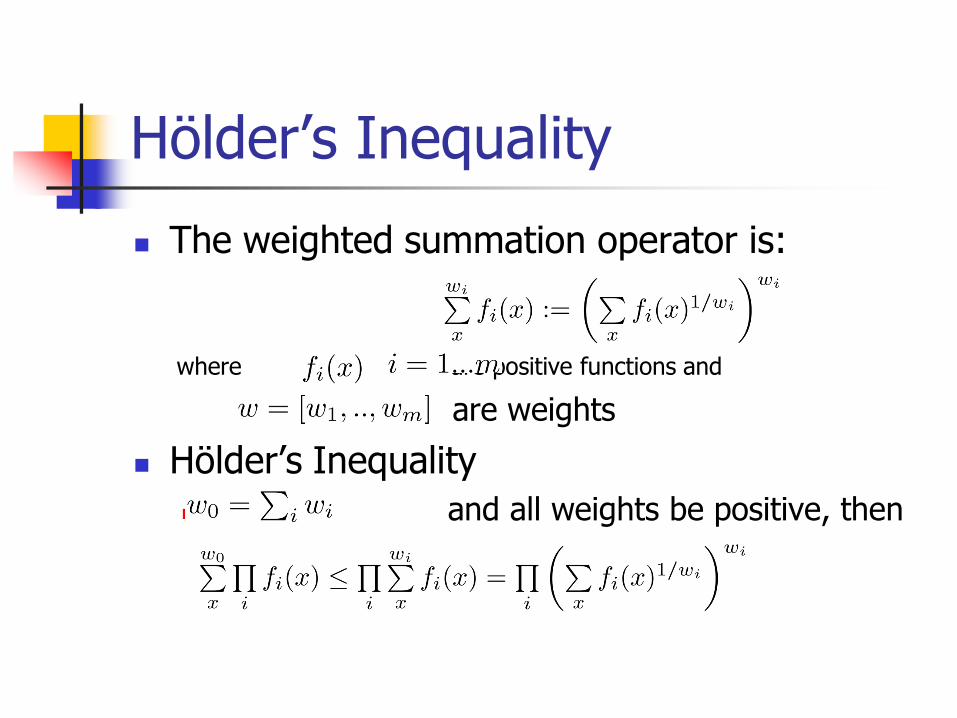
Hölder’s Inequality
The weighted summation operator is:
where , are positive functions and
are weights
Hölder’s Inequality
Let and all weights be positive, then
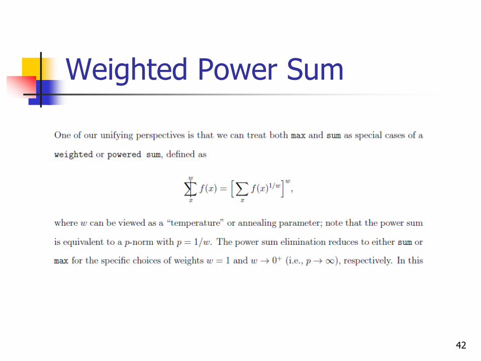
Weighted Power Sum
42

Holder Inequality
43
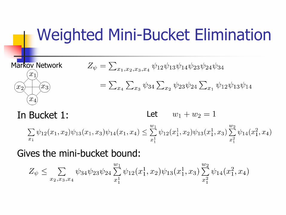
Weighted Mini-Bucket Elimination
Markov Network
In Bucket 1: Let
Gives the mini-bucket bound:
Weighted Mini-Bucket Elimination Markov Network
In Bucket 1:
Let
Gives the mini-bucket bound:
What happens when?
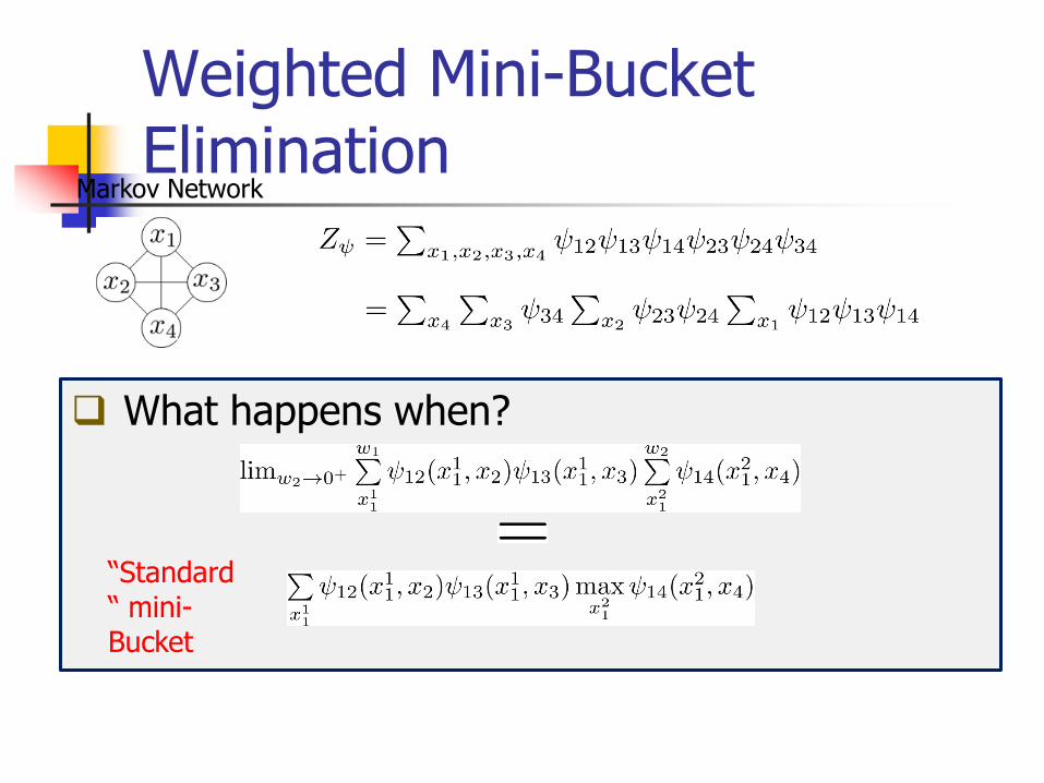
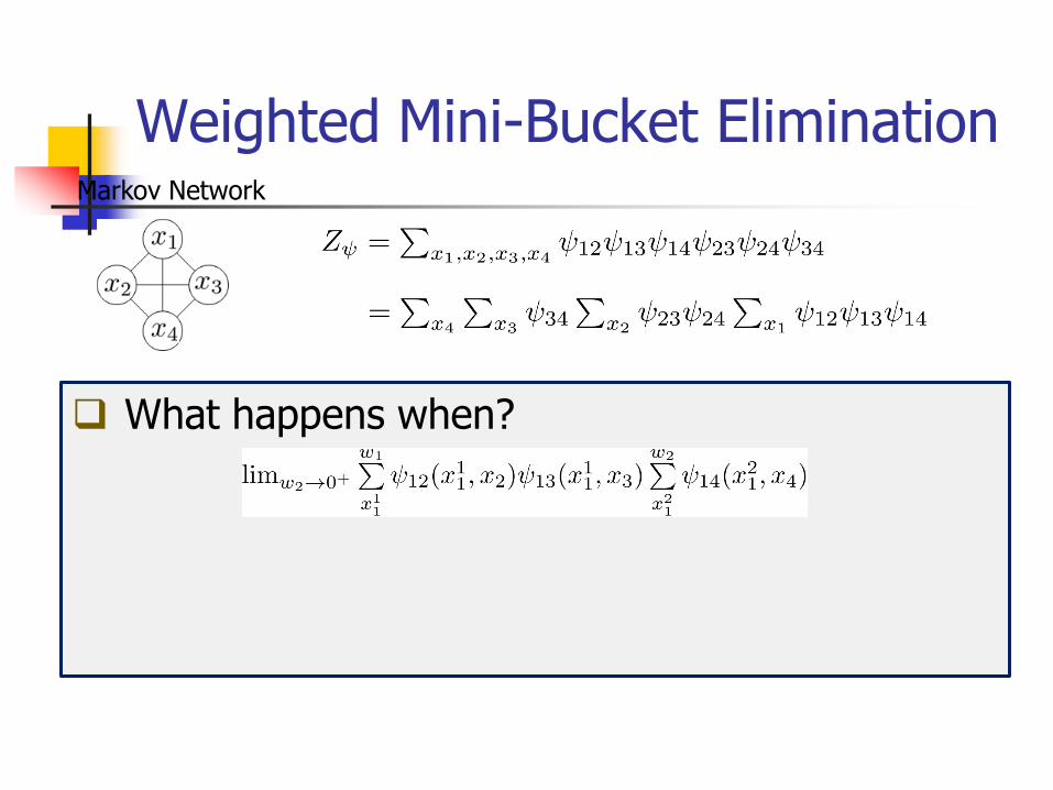
Weighted Mini-Bucket Elimination
Markov Network
In Bucket 1:
Let
Gives the mini-bucket bound:
What happens when?
“Standard “ mini-Bucket
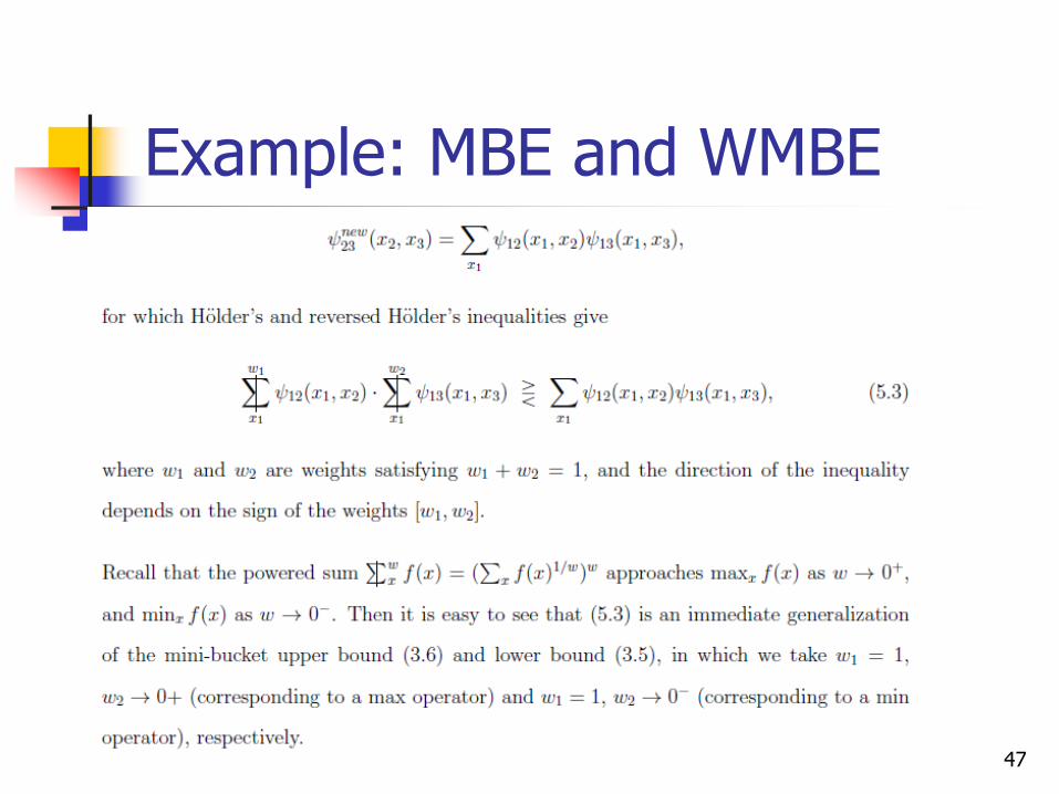
Example: MBE and WMBE
47
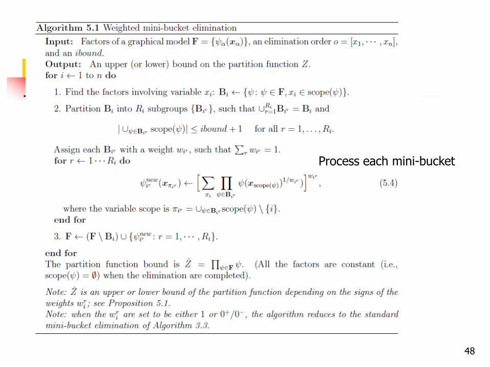
48
Process each mini-bucket
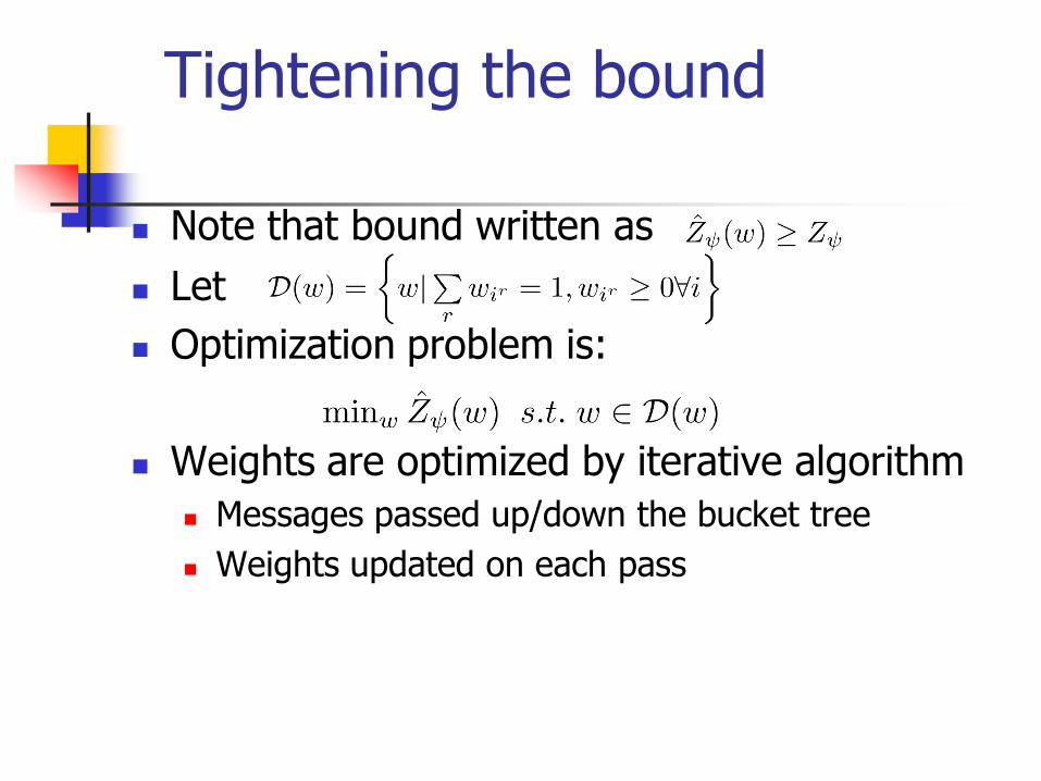
Tightening the bound
Note that bound written as
Let
Optimization problem is:
Weights are optimized by iterative algorithm
Messages passed up/down the bucket tree
Weights updated on each pass
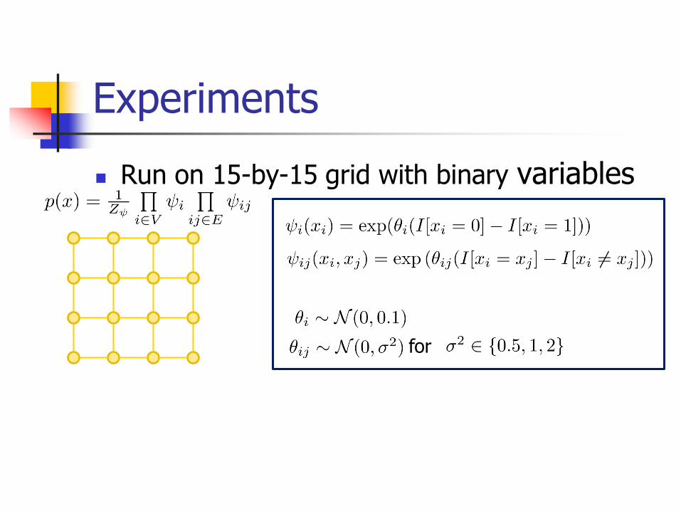
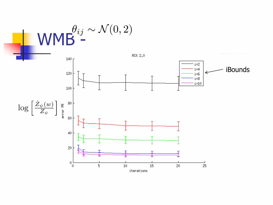
Experiments
Run on 15-by-15 grid with binary variables
for

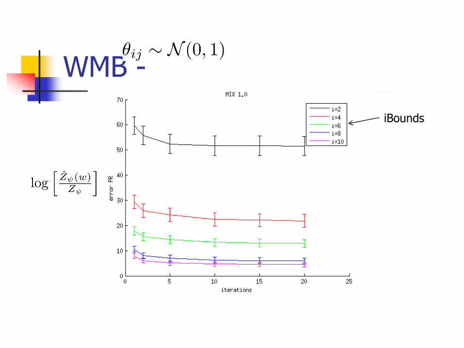
WMB -
iBounds
WMB -
iBounds
WMB -
iBounds
Summary
Variational methods formulate inference as an optimization problem
e.g. given p, find distribution in Q closest to p
Provides new perspective for analysis
e.g. equivalence between fixed points of sum-product message passing and stationary points
Lead to development of many new algorithms
e.g. Liu & Ihler’s weighted mini-bucket