Embed Size (px)
Citation preview

© 2009 Simão et al. Slide 1
Approximate Dynamic Programming CapturesFleet Operations for Schneider National
Daniel H. Wagner Prize for Excellence in O.R. Practice 2009 INFORMS Conference
San DiegoOctober 12, 2009
H. Simão, A. George, W. PowellPrinceton University
J. Day, J. Nienow, T. GiffordSchneider National
© 2009 Simão et al. Slide 2
The operational problemModeling and optimizationAlgorithmic challenges Aggregation Stepsizes Pattern matching
Calibration and validation Policy studies
Outline

© 2009 Simão et al. Slide 3
The operational problemModeling and optimizationAlgorithmic challenges Aggregation Stepsizes Pattern matching
Calibration and validation Policy studies
Outline

© 2009 Simão et al. Slide 4
Schneider National
One of the largest truckload carriers in the U.S.Manages fleet of over 15,000 drivers

© 2009 Simão et al. Slide 5
The operational problem
The one-way service network» 6,500 drivers
• National and regional• Independent owner-operators and company
employees• Solos and teams
» 50,000 loads moved over 4 week period• Regional and transcontinental• Domestic and Canadian
» Schneider must balance:• Empty miles• Customer service• Getting drivers home• Driver regulations

© 2009 Simão et al. Slide 6
• Effect of changes in driver regulations• Policies for driver domiciling/hiring• Policies for getting drivers home• Changes in rules for handling Canadian drivers• Impact of changes in policies for pickup and delivery appointments

© 2009 Simão et al. Slide 7
The operational problemModeling and optimizationAlgorithmic challenges Aggregation Stepsizes Pattern matching
Calibration and validation Policy studies
Outline
© 2009 Simão et al. Slide 8
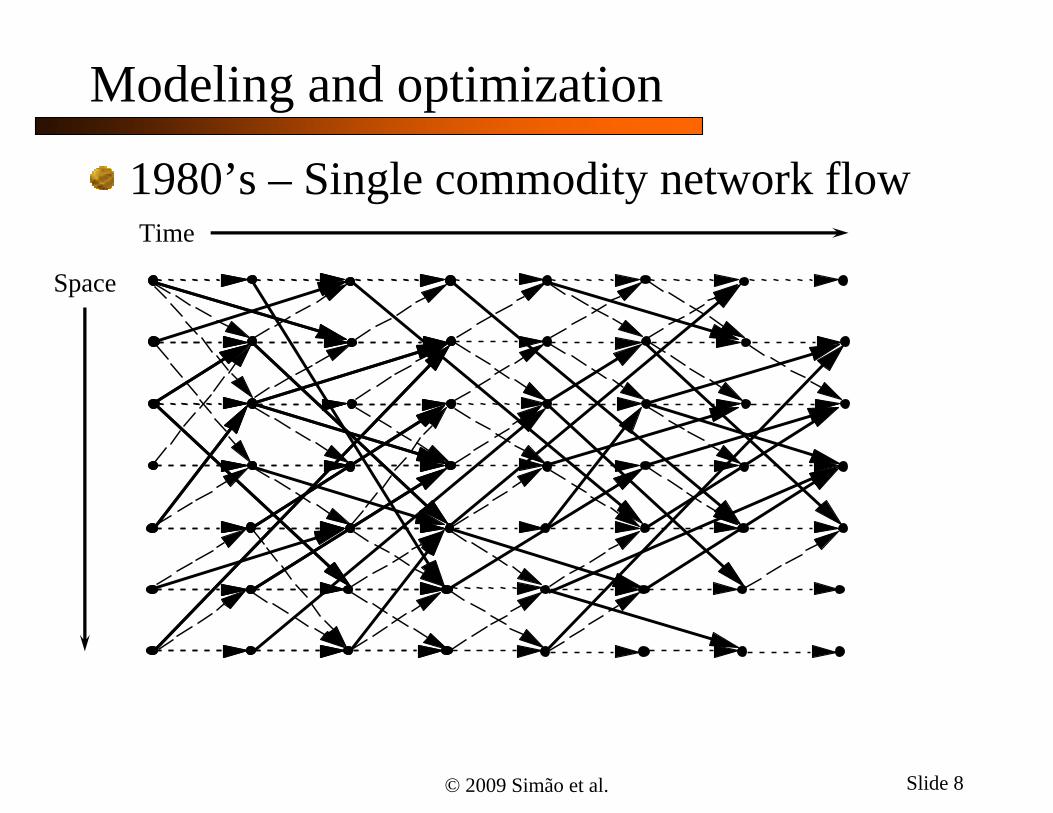
Modeling and optimization
1980’s – Single commodity network flowTime
Space
© 2009 Simão et al. Slide 9
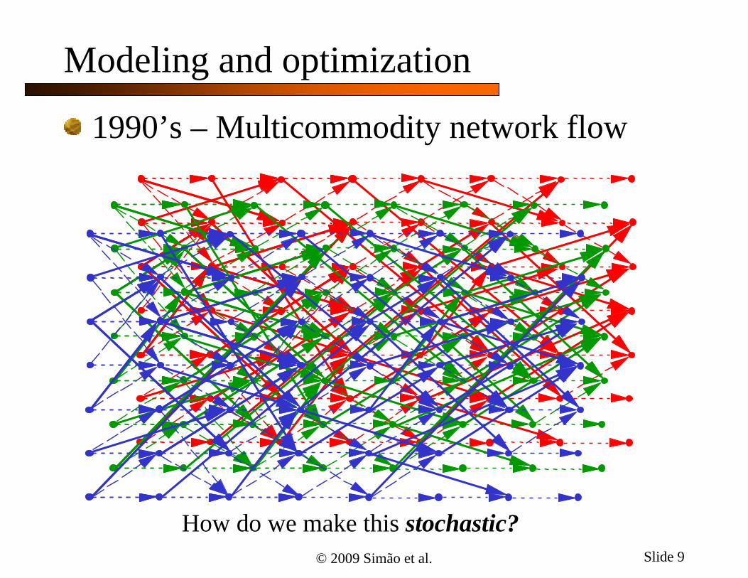
Modeling and optimization
1990’s – Multicommodity network flow
How do we make this stochastic?
© 2009 Simão et al. Slide 10
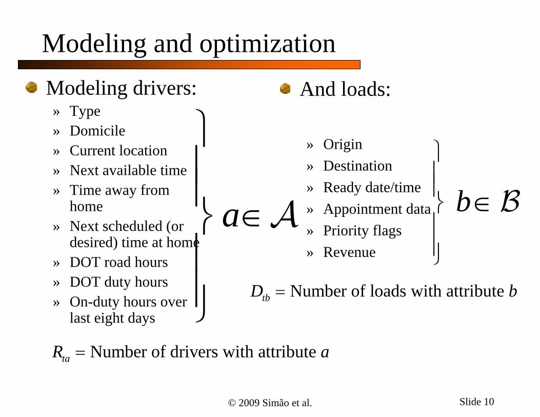
Modeling and optimizationModeling drivers:» Type» Domicile» Current location» Next available time» Time away from
home» Next scheduled (or
desired) time at home» DOT road hours» DOT duty hours» On-duty hours over
last eight days
Number of drivers with attribute taR a
a
And loads:
» Origin» Destination» Ready date/time» Appointment data» Priority flags» Revenue
b
Number of loads with attribute tbD b
© 2009 Simão et al. Slide 11
Modeling and optimization
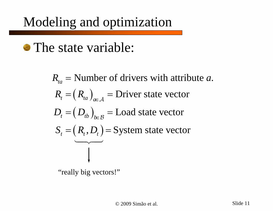
The state variable:
Number of drivers with attribute .Driver state vector
Load state vector
, System state vector
ta
t ta a
t tb b
t t t
R aR R
D D
S R D
“really big vectors!”
© 2009 Simão et al. Slide 12
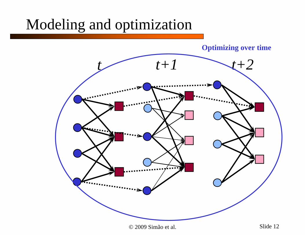
Modeling and optimization
t t+1 t+2Optimizing over time

© 2009 Simão et al. Slide 13
Modeling and optimization
We can formulate the problem as a dynamic program:
1 1
1 1
Solve:
( ) max ( , ) |
where , ,
t t x t t t t t t
Mt t t t
V S C S x E V S S
S S S x W
• The curses of dimensionality State space Outcome space Decision space
• The computational challenge:
How do we find ? 1 1( )t tV S
How do we compute the expectation?
How do we find the optimal solution?

© 2009 Simão et al. Slide 14
Modeling and optimization
Algorithmic strategy using approximate dynamic programming:
1) Eliminate the expectation using the concept of the post-decision state variable
2) Replace the value function with an approximation
3) Design an efficient strategy for learning the value of being in a very high-dimensional state

© 2009 Simão et al. Slide 15Slide 15
Pre- and post-decision states
( , )t t tS R D
The pre-decision state: drivers and loads

© 2009 Simão et al. Slide 16Slide 16
, ( , )x M xt t tS S S x
Pre- and post-decision states
The post-decision state - drivers and loads after a decision is made:
© 2009 Simão et al. Slide 17Slide 17
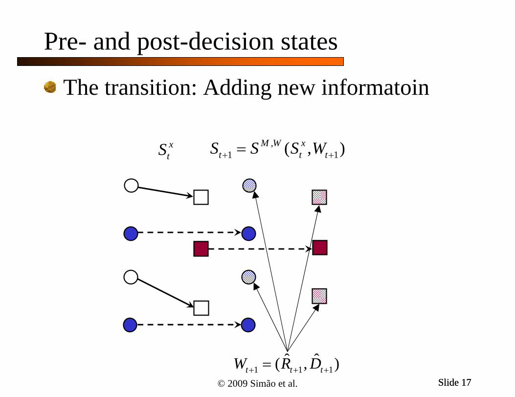
Pre- and post-decision states
1 1 1ˆ ˆ( , )t t tW R D
xtS ,
1 1( , )M W xt t tS S S W
The transition: Adding new informatoin

© 2009 Simão et al. Slide 18Slide 18
Pre- and post-decision states
1tS
The next pre-decision state

© 2009 Simão et al. Slide 19
We use the post-decision state to break Bellman’s equation into two steps» A deterministic optimization problem
• We can solve this using commercial solvers such as CPLEX
» An expectation
• We will approximate this using statistical and/or machine learning techniques
( ) max ( , ) ( , ) x xt t x t t t t t t tV S C S x V S S x
1 1( ) ( ) |x x xt t t t tV S E V S S
Modeling and optimization
© 2009 Simão et al. Slide 20
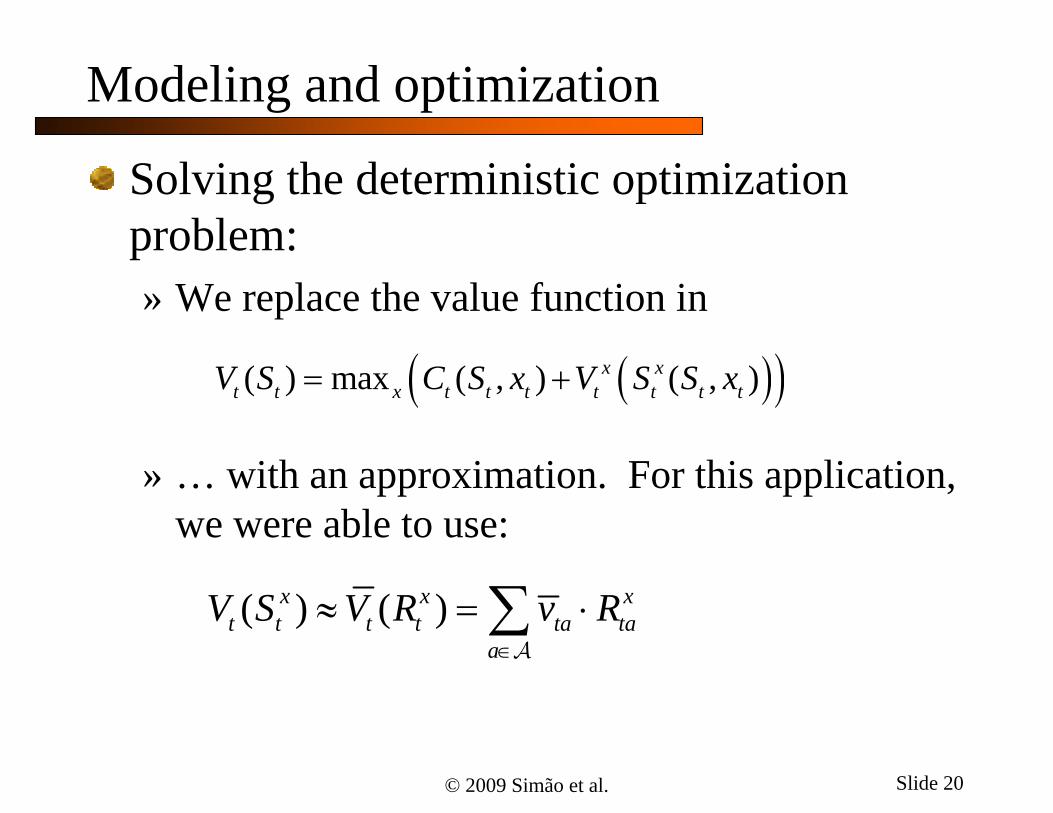
Solving the deterministic optimization problem:» We replace the value function in
» … with an approximation. For this application, we were able to use:
( ) max ( , ) ( , ) x xt t x t t t t t t tV S C S x V S S x
( ) ( )x x xt t t t ta ta
a
V S V R v R
Modeling and optimization
© 2009 Simão et al. Slide 21Slide 21
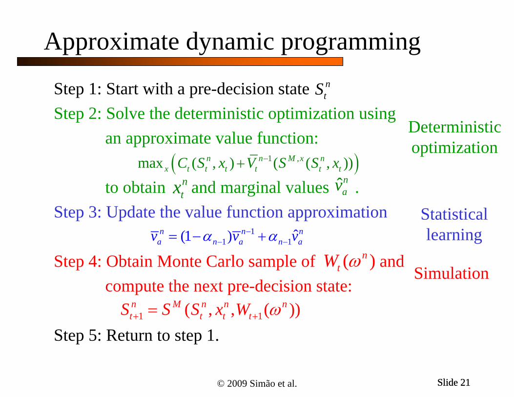
Approximate dynamic programming
Step 1: Start with a pre-decision state Step 2: Solve the deterministic optimization using
an approximate value function:
to obtain and marginal values . Step 3: Update the value function approximation
Step 4: Obtain Monte Carlo sample of andcompute the next pre-decision state:
Step 5: Return to step 1.
11 1 ˆ(1 )n n n
a n a n av v v
1 ,max ( , ) ( ( , )) n n M x nx t t t t t tC S x V S S x
ntx
ntS
( )ntW
1 1( , , ( ))n M n n nt t t tS S S x W
Simulation
Deterministicoptimization
Statisticallearning
ˆnav

© 2009 Simão et al. Slide 22
t
Modeling and optimization

© 2009 Simão et al. Slide 23
Modeling and optimization

© 2009 Simão et al. Slide 24
Modeling and optimization
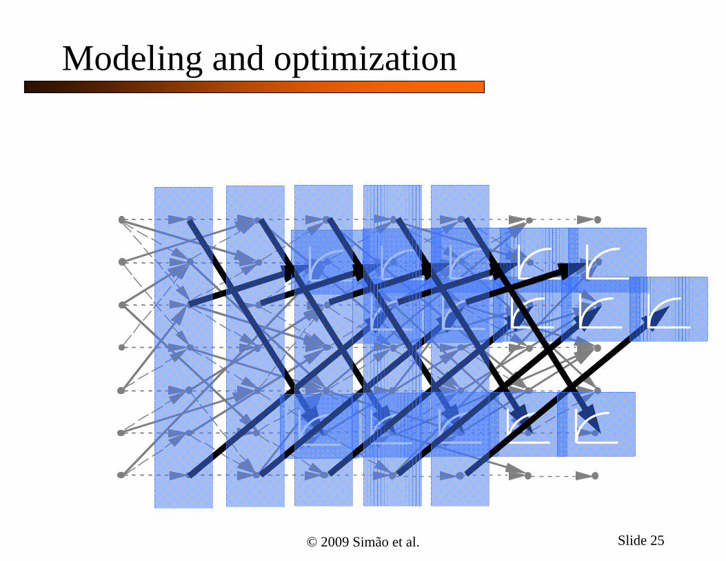
© 2009 Simão et al. Slide 25
Modeling and optimization
© 2009 Simão et al. Slide 26
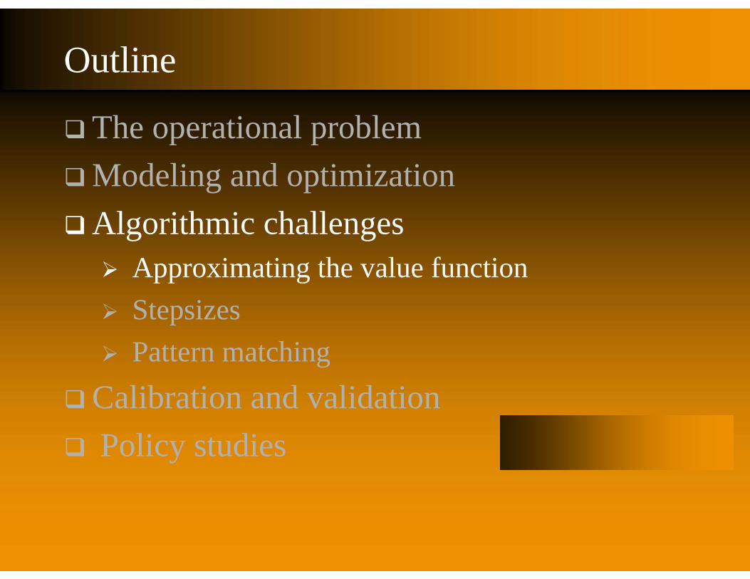
The operational problemModeling and optimizationAlgorithmic challenges Approximating the value function Stepsizes Pattern matching
Calibration and validation Policy studies
Outline

© 2009 Simão et al. Slide 27
Approximating the value function
Our optimization problem at time t looks like:
» For this project, we had to develop novel machine learning strategies to estimate this function.
( ) max ( , ) xt t x t t t ta ta
aV S C S x v R
There are a lot of these attributes!

© 2009 Simão et al. Slide 28
Different levels of aggregation:
TimeRegion Location
Type
33,264
a
672
TimeArea Location
TimeRe gion Location
5,544
TimeRegion LocationRegion Domicile
Type
3,293,136
Approximating the value function

© 2009 Simão et al. Slide 29
Adaptive hierarchical estimation procedure developed as part of this project (George, Powell and Kulkarni, 2008)» Use weighted sum across different levels of aggregation.
( ) ( ) ( )
12( ) ( ) ( )
1
where
g g ga a a a
g g
g g ga a a
v w v w
w Var v
Estimate of bias
Both can be computed using simple recursive formulas.
Estimate of variance - 2 ( )( ) ga
Approximating the value function
George, A., W.B. Powell and S. Kulkarni, “Value Function Approximation Using Hierarchical Aggregation for Multiattribute Resource Management,” Journal of Machine Learning Research, Vol. 9, pp. 2079-2111 (2008).

© 2009 Simão et al. Slide 30
0
0.05
0.1
0.15
0.2
0.25
0.3
0.35
0 200 400 600 800 1000 1200
Iteration
Wei
ghts
Iterations
Wei
ghts
1
32
4
5
Aggregation level
67
Average weight on most disaggregate level
Average weight on most aggregate levels
Approximating the value function

© 2009 Simão et al. Slide 31
1400000
1450000
1500000
1550000
1600000
1650000
1700000
1750000
1800000
1850000
1900000
0 100 200 300 400 500 600 700 800 900 1000
Iterations
Obj
ectiv
e fu
nctio
n
Aggregate
Disaggregate
Approximating the value function

© 2009 Simão et al. Slide 32
1400000
1450000
1500000
1550000
1600000
1650000
1700000
1750000
1800000
1850000
1900000
0 100 200 300 400 500 600 700 800 900 1000
Iterations
Obj
ectiv
e fu
nctio
n
Weighted Combination
Aggregate
Disaggregate
Approximating the value function

© 2009 Simão et al. Slide 33
The operational problemModeling and optimizationAlgorithmic challenges Approximating the value function Stepsizes Pattern matching
Calibration and validation Policy studies
Outline

© 2009 Simão et al. Slide 34
The role of stepsizes in the value function updating equation:
11 1 ˆ(1 )n n n
a n a n av v v
Updated estimate
The stepsize“Learning rate”
“Smoothing factor”
Stepsizes
Old estimate New observation

© 2009 Simão et al. Slide 35
Even stepsizes which are proven to converge to optimality in the limit can work extremely badly
Smoothed estimate using 1/n
Stepsizes
© 2009 Simão et al. Slide 36
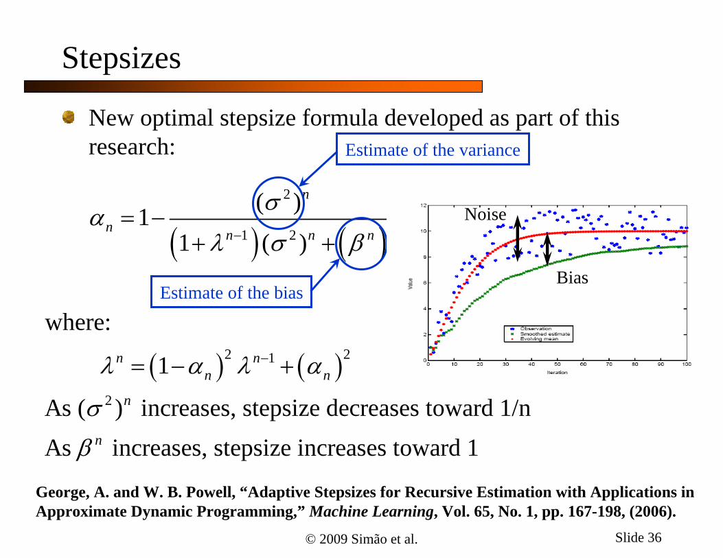
New optimal stepsize formula developed as part of this research:
2
21 2
2 21
2
( )11 ( )
where:
1
As ( ) increases, stepsize decreases toward 1/nAs increases, stepsize increases toward 1
n
n n n n
n nn n
n
n
Estimate of the variance
Estimate of the biasBias
Noise
Stepsizes
George, A. and W. B. Powell, “Adaptive Stepsizes for Recursive Estimation with Applications in Approximate Dynamic Programming,” Machine Learning, Vol. 65, No. 1, pp. 167-198, (2006).
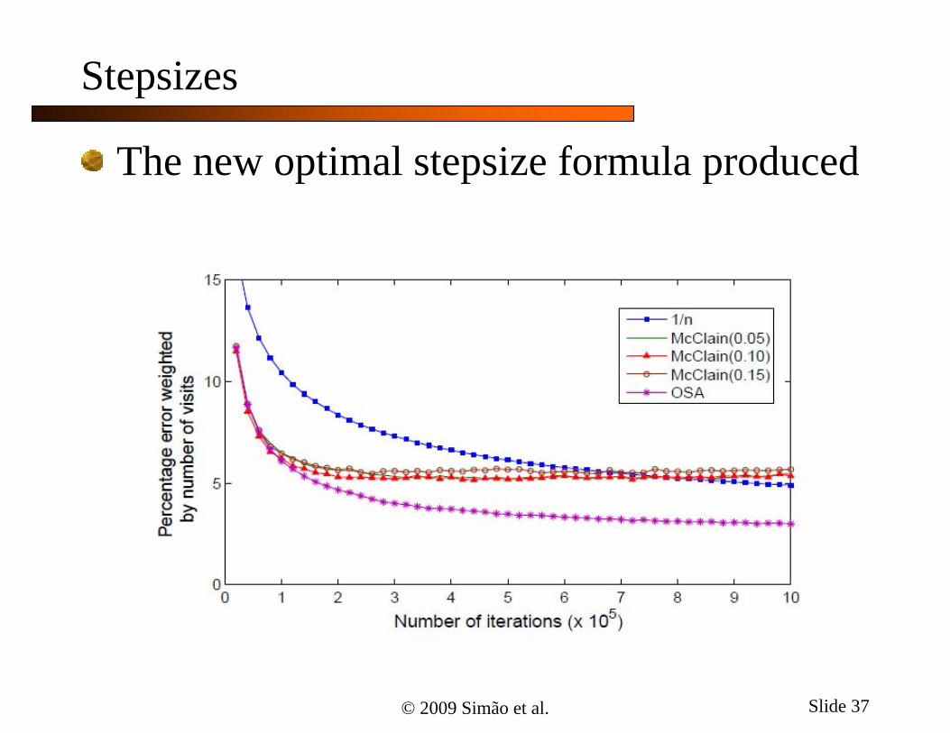
© 2009 Simão et al. Slide 37
Stepsizes
The new optimal stepsize formula produced
© 2009 Simão et al. Slide 38
The operational problemModeling and optimizationAlgorithmic challenges Approximating the value function Stepsizes Pattern matching
Calibration and validation Policy studies
Outline

© 2009 Simão et al. Slide 39
Pattern matching
There are certain corporate behaviors that are difficult to match with engineering rules:
» At Schneider, drivers working in teams have to be assigned to longer loads, on average
» Drivers that own their equipment have the second-longest average length of haul
» Single drivers using company-owned equipment move loads which, on average, are the shortest
Pattern matching offers a viable alternative to incorporate these behaviors into the model

© 2009 Simão et al. Slide 40
The engineering approach
We add in a pattern metric that penalizes deviations from the historical pattern of the distribution of length of haul for each driver type
max ( , ) * ( , )x C S x H xE
0max ( , ) |tx t t t
t
C S x SE
Pattern matching
The difference between the model solution and historical patterns.

© 2009 Simão et al. Slide 41
The engineering approach
We add in a pattern metric that penalizes deviations from the historical pattern of the distribution of length of haul for each driver type
max ( , ) * ( , )x C S x H xE
0max ( , ) |tx t t t
t
C S x SE
Pattern matching
modeldecision variables
Pattern databasefrom history
Scaling parameter

© 2009 Simão et al. Slide 42
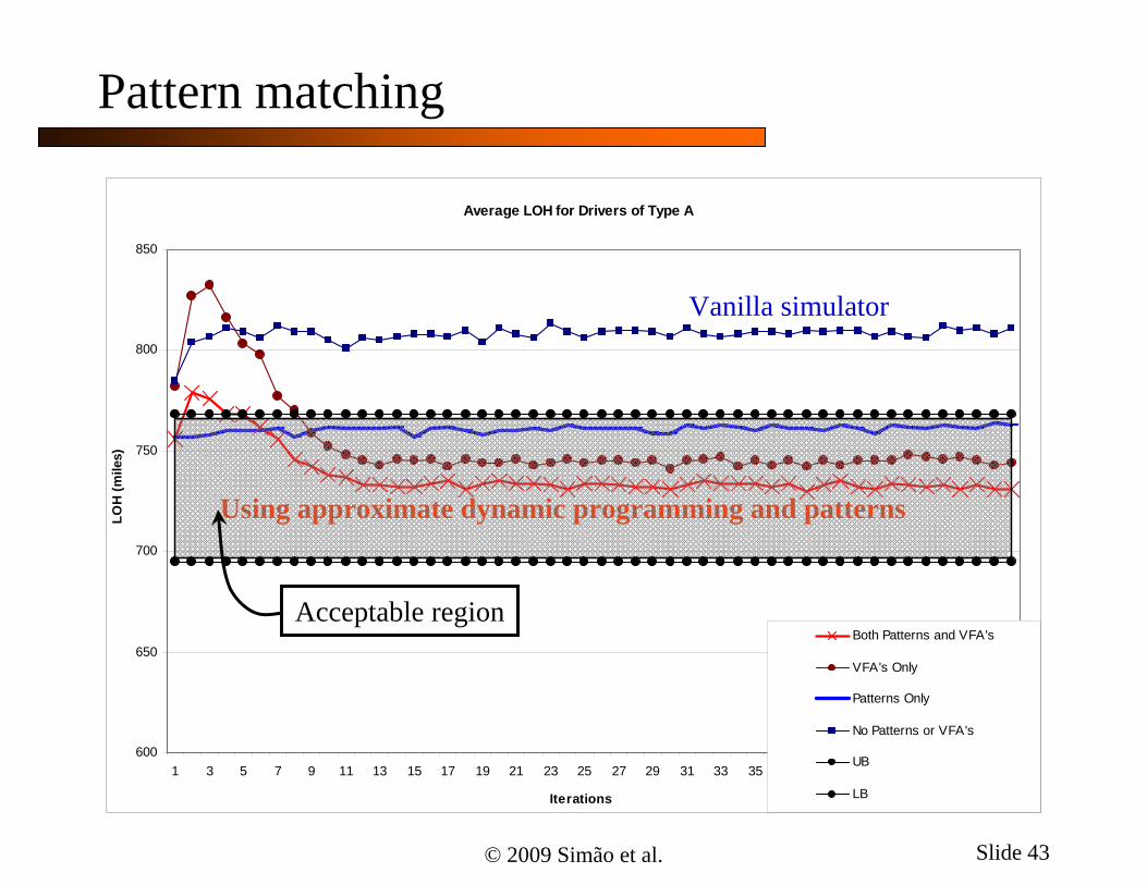
Pattern matching
This strategies builds on a line of research to improve our ability to match patterns using optimization models:
» Marar, A. and W. B. Powell, “Capturing Incomplete Information in Resource Allocation Problems through Numerical Patterns,”European Journal of Operations Research, Vol. 197, No. 1, pp. 50-58 (2009)
» Marar, A. W. B. Powell and S. Kulkarni, “Combining Cost-Based and Rule-Based Knowledge in Complex Resource Allocation Problems,” IIE transactions, Vol. 38 (2), pp. 159-172 2006.
© 2009 Simão et al. Slide 43
Average LOH for Drivers of Type A
600
650
700
750
800
850
1 3 5 7 9 11 13 15 17 19 21 23 25 27 29 31 33 35 37 39 41 43 45 47 49
Iterations
LOH
(mile
s)
Both Patterns and VFA's
VFA's Only
Patterns Only
No Patterns or VFA's
UB
LB
Vanilla simulator
Using approximate dynamic programming and patterns
Acceptable region
Pattern matching

© 2009 Simão et al. Slide 44
The operational problemModeling and optimizationAlgorithmic challenges Aggregation Stepsizes Pattern matching
Calibration and validation Policy studies
Outline

© 2009 Simão et al. Slide 45
0
200
400
600
800
1000
1200
1400
1600
US_SOLO US_IC US_TEAM
LOH
Capacity category
Historical maximum
Simulation
Historical minimum
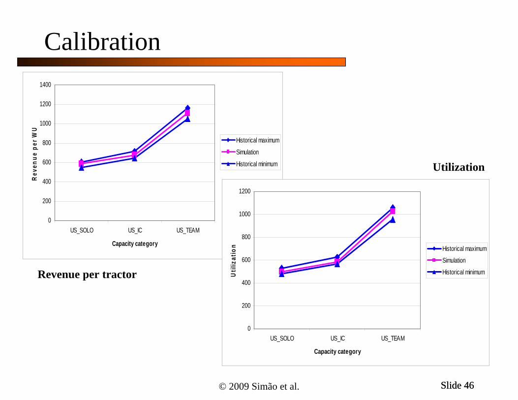
Calibration
Historical min and maxCalibrated model
Matching average length of haul
© 2009 Simão et al. Slide 46Slide 46
0
200
400
600
800
1000
1200
1400
US_SOLO US_IC US_TEAM
Capacity category
Rev
enue
per
WU
Historical maximum
Simulation
Historical minimum
0
200
400
600
800
1000
1200
US_SOLO US_IC US_TEAM
Capacity category
Util
izat
ion Historical maximum
Simulation
Historical minimumRevenue per tractor
Utilization
Calibration

© 2009 Simão et al. Slide 47
Validation
simulation objective function
1800000
1810000
1820000
1830000
1840000
1850000
1860000
1870000
1880000
1890000
1900000
580 590 600 610 620 630 640 650
# of drivers w ith attribute a
s1
s2
s3
s4
s5
s6
s7
s8
s9
s10
avg
pred

© 2009 Simão et al. Slide 48
Validation
simulation objective function
1800000
1810000
1820000
1830000
1840000
1850000
1860000
1870000
1880000
1890000
1900000
580 590 600 610 620 630 640 650
# of drivers w ith attribute a
s1
s2
s3
s4
s5
s6
s7
s8
s9
s10
avg
pred
av

© 2009 Simão et al. Slide 49
Validation
-500
0
500
1000
1500
2000
2500
3000
3500
1 2 3 4 5 6 7 8 9 10 11 12 13 14 15 16 17 18 19 20

© 2009 Simão et al. Slide 50
The operational problemModeling and optimizationAlgorithmic challenges Aggregation Stepsizes Pattern matching
Calibration and validation Policy studies
Outline
© 2009 Simão et al. Slide 51© 2009 Simão et al. Slide 51
Policy studies
Driver Scheduling (Time-at-Home )» Motivation: Scheduling flexibility is a trade-off of
driver quality-of-life and network efficiency. A business plan to allow driver self-scheduling was piloted with potentially promising results. Prior to implementation, better analysis was needed
» Questions: Is this feasible? Do the pilot results scale to the full transportation network? What are the cost impacts?
» Results: Original plan was only feasible at a very high cost ($30M/year). An alternate plan suggested by simulation modeling was implemented at a cost of $6M/year while achieving similar benefits.

© 2009 Simão et al. Slide 52© 2009 Simão et al. Slide 52
Policy studies
Driver Hours-of-Service (HOS) Rules» Motivation: Six years ago the US DOT introduced
significant changes in the driver work schedule rules. Quantitative impact of these changes was hard to determine.
» Questions: What would be the productivity impact of the changes? What steps could be taken to mitigate these effects; i.e., to either lessen or obtain compensation for them.
» Results: The company was able to effectively negotiate adjustments in customer billing rates and freight tendering/handling procedures, leading to margin improvements of 2 to 3%.

© 2009 Simão et al. Slide 53© 2009 Simão et al. Slide 53
Policy studies
Setting Appointments» Motivation: A key challenge in the order booking
process it how to determine both the timing and the flexibility of the load pickup and delivery appointments.
» Questions: What is the operational impact of various different types of appointment criteria?
» Results: Schneider negotiated and adjusted appointment criteria resulting lower customer costs, margin improvement up to10%, and 50% reduction in late deliveries.

© 2009 Simão et al. Slide 54© 2009 Simão et al. Slide 54
Policy studiesCross Border Relay Network» Motivation: New security-increasing border crossing
(US/Canada) procedures were introduced which require special training/identification/certification of cross border drivers.
» Questions: Would a network redesign reducing the number of crossing points and border-crossing drivers be feasible? What would be the cost and service impacts?
» Results: Relying heavily on simulation analysis, a small set of relay points was established, allowing border-crossing to be concentrated with Canadian drivers. The number of drivers who had to be trained/certified was reduced by 91%, with cost avoidance of $3.8M and annual savings of $2.3M.

© 2009 Simão et al. Slide 55© 2009 Simão et al. Slide 55
Policy studiesDriver Domiciles» Motivation: Driver domiciles (home-base) significantly
affect both pay rates and network efficiency. Pre-existing criteria for domicile hiring targets and pay differentials were not based on sound analysis.
» Questions: How should domicile region hiring quotas and pay differentials be set to best balance freight flows with regional employment opportunities.
» Results: Simulator-derived approximate value functions were used to provide estimates of the marginal value of drivers by type and region. These are now used to guide hiring strategies, leading to an estimated annual profit improvement of $5M.
© 2009 Simão et al. Slide 56© 2009 Simão et al. Slide 56
Policy studiesLarge Shipper Request» Motivation: A large shipper asked for tighter time
windows on its approximately 4,500 loads per month delivered by Schneider.
» Questions: What is the cost impact to satisfy this request? How can this impact be justified to the customer?
» Results: Using the simulator, The annual cost increase was estimated to be $1.9M. The shipper subsequently withdrew the request.