Embed Size (px)
Citation preview
Applied Regression Modeling forCross-Section Data
Kosuke Imai
Princeton University
POL573 Quantitative Analysis IIIFall 2013
Kosuke Imai (Princeton) Regression for Cross-Section Data POL573 Fall 2013 1 / 29

Suggested Readings and References
King, 5.7–5.9,Wooldridge, 19.1–19.4Gelman and Hill, Chapter 6McCullagh and Nelder. (1989). Generalized Linear Models.Chapman & Hall. Especially, Chapters 2, 4, 9, and 12.
Kosuke Imai (Princeton) Regression for Cross-Section Data POL573 Fall 2013 2 / 29
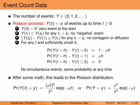
Event Count Data
The number of events: Y ∈ 0,1,2, . . .
Poisson process: Y (t) = # of events up to time t ≥ 01 Y (0) = 0: zero event at the start2 Y (t1) ≤ Y (t2) for any t1 < t2: no “negative” event3 Y (t2)− Y (t1)⊥⊥Y (t1) for any t1 < t2: no contagion or diffusion4 For any t and sufficiently small h,
Pr(Y (t + h)− Y (t) = 0) ≈ 1− µhPr(Y (t + h)− Y (t) = 1) ≈ µhPr(Y (t + h)− Y (t) ≥ 2) ≈ 0
No simultaneous events, same probability at any time
After some math, this leads to the Poisson distribution:
Pr(Y (t) = y) =(µt)y
y !exp(−µt) or Pr(Y = y) =
µy
y !exp(−µ)
Kosuke Imai (Princeton) Regression for Cross-Section Data POL573 Fall 2013 3 / 29
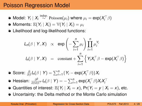
Poisson Regression Model
Model: Yi | Xiindep.∼ Poisson(µi) where µi = exp(X>i β)
Moments: E(Yi | Xi) = V(Yi | Xi) = µi
Likelihood and log-likelihood functions:
Ln(β | Y ,X ) ∝ exp
(−
n∑i=1
µi
)n∏
i=1
µYii
ln(β | Y ,X ) = constant +n∑
i=1
YiX>i β − exp(X>i β)
Score: ∂
∂β ln(β | Y ) =∑n
i=1Yi − exp(X>i β)Xi
Hessian: ∂2
∂β∂β>ln(β | Y ) = −
∑ni=1 exp(X>i β)XiX>i
Quantities of interest: E(Yi | Xi = x), Pr(Yi = y | Xi = x), etc.Uncertainty: the Delta method or the Monte Carlo simulation
Kosuke Imai (Princeton) Regression for Cross-Section Data POL573 Fall 2013 4 / 29
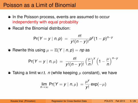
Poisson as a Limit of Binomial
In the Poisson process, events are assumed to occurindependently with equal probabilityRecall the Binomial distribution:
Pr(Y = y | n,p) =n!
y !(n − y)!py (1− p)n−y
Rewrite this using µ = E(Y | n,p) = np as
Pr(Y = y | n, µ) =n!
y !(n − y)!
(µn
)y (1− µ
n
)n−y
Taking a limit w.r.t. n (while keeping µ constant), we have
limn→∞
Pr(Y = y | n, µ) =µy
y !exp(−µ)
Kosuke Imai (Princeton) Regression for Cross-Section Data POL573 Fall 2013 5 / 29
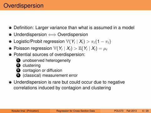
Overdispersion
Definition: Larger variance than what is assumed in a modelUnderdispersion⇐⇒ OverdispersionLogistic/Probit regression V(Yi | Xi) > πi1− πiPoisson regression V(Yi | Xi) > E(Yi | Xi) = µi
Potential sources of overdispersion:1 unobserved heterogeneity2 clustering3 contagion or diffusion4 (classical) measurement error
Underdispersion is rare but could occur due to negativecorrelations induced by contagion and clustering
Kosuke Imai (Princeton) Regression for Cross-Section Data POL573 Fall 2013 6 / 29
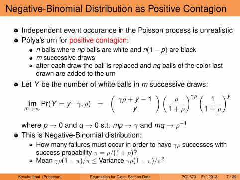
Negative-Binomial Distribution as Positive Contagion
Independent event occurance in the Poisson process is unrealisticPólya’s urn for positive contagion:
n balls where np balls are white and n(1− p) are blackm successive drawsafter each draw the ball is replaced and nq balls of the color lastdrawn are added to the urn
Let Y be the number of white balls in m successive draws:
limm→∞
Pr(Y = y | γ, ρ) =
(γρ+ y − 1
y
)(ρ
1 + ρ
)γρ( 11 + ρ
)y
where p → 0 and q → 0 s.t. mp → γ and mq → ρ−1
This is Negative-Binomial distribution:How many failures must occur in order to have γρ successes withsuccess probability π = ρ/(1 + ρ)?Mean γρ(1− π)/π ≤ Variance γρ(1− π)/π2
Kosuke Imai (Princeton) Regression for Cross-Section Data POL573 Fall 2013 7 / 29
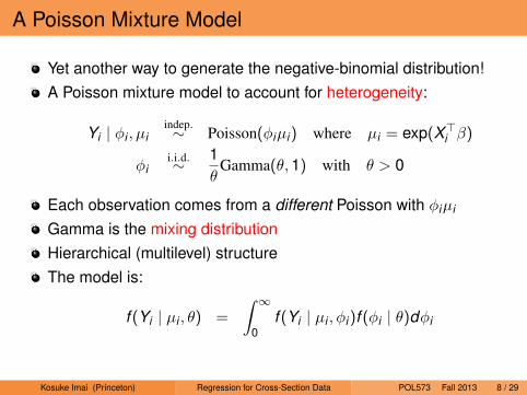
A Poisson Mixture Model
Yet another way to generate the negative-binomial distribution!A Poisson mixture model to account for heterogeneity:
Yi | φi , µiindep.∼ Poisson(φiµi) where µi = exp(X>i β)
φii.i.d.∼ 1
θGamma(θ,1) with θ > 0
Each observation comes from a different Poisson with φiµi
Gamma is the mixing distributionHierarchical (multilevel) structureThe model is:
f (Yi | µi , θ) =
∫ ∞0
f (Yi | µi , φi)f (φi | θ)dφi
Kosuke Imai (Princeton) Regression for Cross-Section Data POL573 Fall 2013 8 / 29
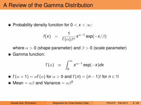
A Review of the Gamma Distribution
Probability density function for 0 < x <∞:
f (x) =1
Γ(α)βαxα−1 exp(−x/β)
where α > 0 (shape parameter) and β > 0 (scale parameter)Gamma function:
Γ(α) ≡∫ ∞
0xα−1 exp(−x)dx
Γ(α + 1) = αΓ(α) for α > 0 and Γ(n) = (n − 1)! for n ∈ NMean = αβ and Variance = αβ2
Kosuke Imai (Princeton) Regression for Cross-Section Data POL573 Fall 2013 9 / 29
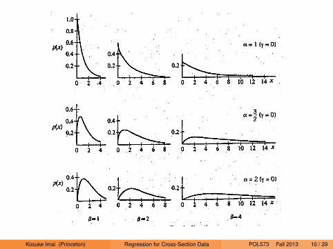
Kosuke Imai (Princeton) Regression for Cross-Section Data POL573 Fall 2013 10 / 29
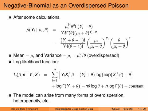
Negative-Binomial as an Overdispersed Poisson
After some calculations,
p(Yi | µi , θ) =µYi
i θθΓ(Yi + θ)
Yi !Γ(θ)(µi + θ)Yi+θ
=(Yi + θ − 1)!
Yi !(θ − 1)!
(µi
µi + θ
)Yi(
θ
µi + θ
)θMean = µi and Variance = µi + µ2
i /θ (overdispersed!)Log-likelihood function:
ln(β, θ | Y ,X ) =n∑
i=1
[YiX>i β − (Yi + θ) logexp(X>i β) + θ
+ log Γ(Yi + θ)]−nθ log θ + n log Γ(θ) + constant
The model can arise from many forms of overdispersion,heterogeneity, etc.
Kosuke Imai (Princeton) Regression for Cross-Section Data POL573 Fall 2013 11 / 29
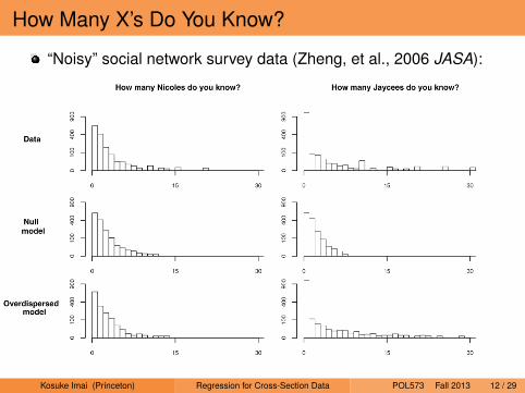
How Many X’s Do You Know?
“Noisy” social network survey data (Zheng, et al., 2006 JASA):
412 Journal of the American Statistical Association, June 2006
count data. As is standard in generalized linear models (e.g.,McCullagh and Nelder 1989), we use “overdispersion” to referto data with more variance than expected under a null model,and also as a parameter in an expanded model that captures thisvariation.
Comparison of the Three Models Using “How Many X’s DoYou Know?” Count Data. Figure 1 shows some of the data—the distributions of responses, yik, to the questions “How manypeople named Nicole do you know?” and “How many Jayceesdo you know?,” along with the expected distributions underthe Erdös–Renyi model, our null model, and our overdispersedmodel. (“Jaycees” are members of the Junior Chamber of Com-merce, a community organization of people age 21–39. Becausethe Jaycees are a social organization, it makes sense that noteveryone has the same propensity to know one—people whoare in the social circle of one Jaycee are particularly likely toknow others.) We chose these two groups to plot because theyare close in average number known (.9 Nicoles, 1.2 Jaycees) buthave much different distributions; the distribution for Jayceeshas much more variation, with more zero responses and moreresponses in the upper tail.
The three models can be written as follows in statistical no-tation as yik ∼ Poisson(λik), with increasingly general formsfor λik:
Erdös–Renyi model: λik= abk,
Our null model: λik= aibk,
Our overdispersed model: λik= aibkgik.
Comparing the models, the Erdös–Renyi model implies aPoisson distribution for the responses to each “How many X’sdo you know?” question, whereas the other models allow formore dispersion. The null model turns out to be a much bet-ter fit to the Nicoles than to the Jaycees, indicating that thereis comparably less variation in the propensity to form ties withNicoles than with Jaycees. The overdispersed model fits bothdistributions reasonably well and captures the difference be-tween the patterns of the acquaintance with Nicoles and Jayceesby allowing individuals to differ in their relative propensities toform ties to people in specific groups (gik). As we show, usingthe overdispersed model, both variation in social network sizesand variations in relative propensities to form ties to specificgroups can be estimated from the McCarty et al. data.
Figure 1. Histograms (on the square-root scale) of Responses to “How Many Persons Do You Know Named Nicole?” and “How Many JayceesDo You Know?” From the McCarty et al. Data and From Random Simulations Under Three Fitted Models: The Erdös–Renyi Model (completelyrandom links), Our Null Model (some people more gregarious than others, but uniform relative propensities for people to form ties to all groups),and Our Overdispersed Model (variation in gregariousness and variation in propensities to form ties to different groups). Each model shows moredispersion than the one above, with the overdispersed model fitting the data reasonably well. The propensities to form ties to Jaycees show muchmore variation than the propensities to form ties to Nicoles, and hence the Jaycees counts are much more overdispersed. (The data also showminor idiosyncrasies such as small peaks at the responses 10, 15, 20, and 25. All values >30 have been truncated at 30.) We display the resultson square-root scale to more clearly reveal patterns in the tails.
Kosuke Imai (Princeton) Regression for Cross-Section Data POL573 Fall 2013 12 / 29
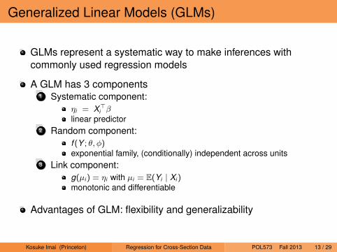
Generalized Linear Models (GLMs)
GLMs represent a systematic way to make inferences withcommonly used regression models
A GLM has 3 components1 Systematic component:
ηi = X>i βlinear predictor
2 Random component:f (Y ; θ, φ)exponential family, (conditionally) independent across units
3 Link component:g(µi) = ηi with µi = E(Yi | Xi)monotonic and differentiable
Advantages of GLM: flexibility and generalizability
Kosuke Imai (Princeton) Regression for Cross-Section Data POL573 Fall 2013 13 / 29
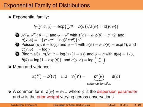
Exponential Family of Distributions
Exponential family:
fY (y ; θ, φ) = exp(yθ − b(θ))/a(φ) + c(y , φ)
1 N (µ, σ2): θ = µ and φ = σ2 with a(φ) = φ,b(θ) = θ2/2, andc(y , φ) = −y2/σ2 + log(2πσ2)/2
2 Poisson(µ): θ = logµ and φ = 1 with a(φ) = φ,b(θ) = exp(θ), andc(y , φ) = − log y !
3 Binomial(π,n)/n: θ = logπ/(1− π) and φ = n with a(φ) = 1/φ,b(θ) = log1 + exp(θ), and c(y , φ) = log
(n
ny
)Mean and variance:
E(Y ) = b′(θ) and V(Y ) = b′′(θ)︸ ︷︷ ︸variance function
a(φ)
A common form: a(φ) = φ/ω where φ is the dispersion parameterand ω is the prior weight varying across observations
Kosuke Imai (Princeton) Regression for Cross-Section Data POL573 Fall 2013 14 / 29
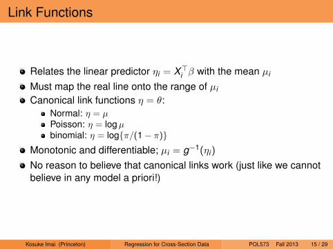
Link Functions
Relates the linear predictor ηi = X>i β with the mean µi
Must map the real line onto the range of µi
Canonical link functions η = θ:Normal: η = µPoisson: η = logµbinomial: η = logπ/(1− π)
Monotonic and differentiable; µi = g−1(ηi)
No reason to believe that canonical links work (just like we cannotbelieve in any model a priori!)
Kosuke Imai (Princeton) Regression for Cross-Section Data POL573 Fall 2013 15 / 29
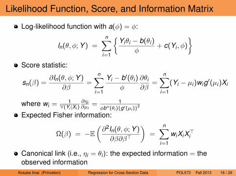
Likelihood Function, Score, and Information Matrix
Log-likelihood function with a(φ) = φ:
ln(θ, φ; Y ) =n∑
i=1
Yiθi − b(θi)
φ+ c(Yi , φ)
Score statistic:
sn(β) =∂ln(θ, φ; Y )
∂β=
n∑i=1
Yi − b′(θi)
φ
∂θi
∂β=
n∑i=1
(Yi − µi)wig′(µi)Xi
where wi = 1V(Yi |Xi )
∂ηi∂µi
= 1φb′′(θi )g′(µi )2
Expected Fisher information:
Ω(β) = −E(∂2ln(θ, φ; Y )
∂β∂β>
)=
n∑i=1
wiXiX>i
Canonical link (i.e., ηi = θi ): the expected information = theobserved information
Kosuke Imai (Princeton) Regression for Cross-Section Data POL573 Fall 2013 16 / 29
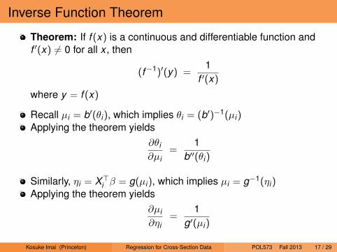
Inverse Function Theorem
Theorem: If f (x) is a continuous and differentiable function andf ′(x) 6= 0 for all x , then
(f−1)′(y) =1
f ′(x)
where y = f (x)
Recall µi = b′(θi), which implies θi = (b′)−1(µi)Applying the theorem yields
∂θi
∂µi=
1b′′(θi)
Similarly, ηi = X>i β = g(µi), which implies µi = g−1(ηi)Applying the theorem yields
∂µi
∂ηi=
1g′(µi)
Kosuke Imai (Princeton) Regression for Cross-Section Data POL573 Fall 2013 17 / 29
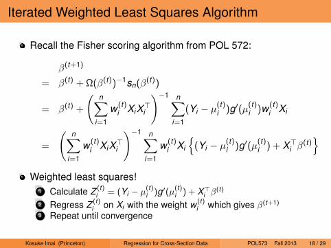
Iterated Weighted Least Squares Algorithm
Recall the Fisher scoring algorithm from POL 572:
β(t+1)
= β(t) + Ω(β(t))−1sn(β(t))
= β(t) +
(n∑
i=1
w (t)i XiX>i
)−1 n∑i=1
(Yi − µ(t)i )g′(µ(t)i )w (t)
i Xi
=
(n∑
i=1
w (t)i XiX>i
)−1 n∑i=1
w (t)i Xi
(Yi − µ
(t)i )g′(µ(t)i ) + X>i β
(t)
Weighted least squares!1 Calculate Z (t)
i = (Yi − µ(t)i )g′(µ
(t)i ) + X>
i β(t)
2 Regress Z (t)i on Xi with the weight w (t)
i which gives β(t+1)
3 Repeat until convergence
Kosuke Imai (Princeton) Regression for Cross-Section Data POL573 Fall 2013 18 / 29
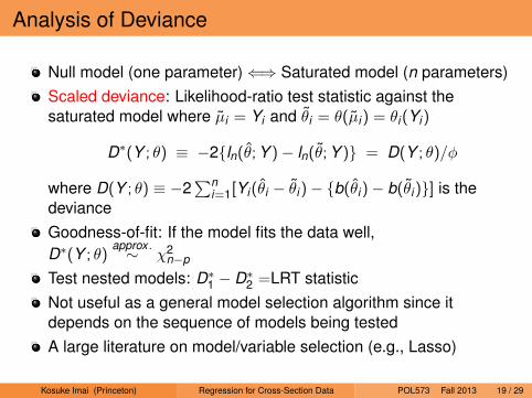
Analysis of Deviance
Null model (one parameter)⇐⇒ Saturated model (n parameters)Scaled deviance: Likelihood-ratio test statistic against thesaturated model where µi = Yi and θi = θ(µi) = θi(Yi)
D∗(Y ; θ) ≡ −2ln(θ; Y )− ln(θ; Y ) = D(Y ; θ)/φ
where D(Y ; θ) ≡ −2∑n
i=1[Yi(θi − θi)− b(θi)− b(θi)] is thedevianceGoodness-of-fit: If the model fits the data well,D∗(Y ; θ)
approx .∼ χ2n−p
Test nested models: D∗1 − D∗2 =LRT statisticNot useful as a general model selection algorithm since itdepends on the sequence of models being testedA large literature on model/variable selection (e.g., Lasso)
Kosuke Imai (Princeton) Regression for Cross-Section Data POL573 Fall 2013 19 / 29
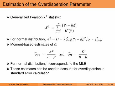
Estimation of the Overdispersion Parameter
Generalized Pearson χ2 statistic:
X 2 ≡n∑
i=1
(Yi − µi)2
b′′(θi)
For normal distribution, X 2 = D =∑n
i=1(Yi − µi)2/φ ∼ χ2
n−p
Moment-based estimates of φ:
φX 2 =X 2
n − pand φD =
Dn − p
For normal distribution, it corresponds to the MLEThese estimates can be used to account for overdispersion instandard error calculation
Kosuke Imai (Princeton) Regression for Cross-Section Data POL573 Fall 2013 20 / 29
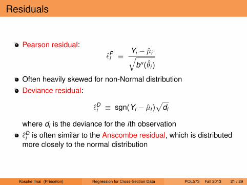
Residuals
Pearson residual:εPi ≡
Yi − µi√b′′(θi)
Often heavily skewed for non-Normal distributionDeviance residual:
εDi ≡ sgn(Yi − µi)√
di
where di is the deviance for the i th observationεDi is often similar to the Anscombe residual, which is distributedmore closely to the normal distribution
Kosuke Imai (Princeton) Regression for Cross-Section Data POL573 Fall 2013 21 / 29
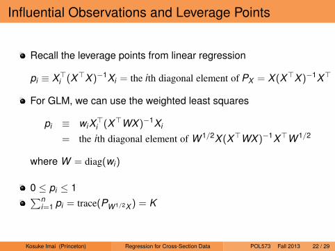
Influential Observations and Leverage Points
Recall the leverage points from linear regression
pi ≡ X>i (X>X )−1Xi = the i th diagonal element of PX = X (X>X )−1X>
For GLM, we can use the weighted least squares
pi ≡ wiX>i (X>WX )−1Xi
= the i th diagonal element of W 1/2X (X>WX )−1X>W 1/2
where W = diag(wi)
0 ≤ pi ≤ 1∑ni=1 pi = trace(PW 1/2X ) = K
Kosuke Imai (Princeton) Regression for Cross-Section Data POL573 Fall 2013 22 / 29
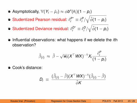
Asymptotically, V(Yi − µi) ≈ φb′′(θi)(1− pi)
Studentized Pearson residual: εP∗
i ≡ εPi /√φ(1− pi)
Studentized Deviance residual: εD∗
i ≡ εDi /√φ(1− pi)
Influential observations: what happens if we delete the i thobservation?
β(i) ≈ β −√
wi(X>WX )−1XiεPi
(1− pi)
Cook’s distance:
Di ≡(β(i) − β)(X>WX )−1(β(i) − β)
φK
Kosuke Imai (Princeton) Regression for Cross-Section Data POL573 Fall 2013 23 / 29
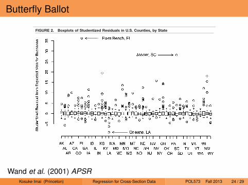
Butterfly Ballot
County in Kansas, which are in contiguous clusters withunusually large numbers of Buchanan votes. PBC hasthe largest residual and Jasper County the secondlargest, whether we use one or two principal compo-nents to represent the demographic variables. Withthree principal components, PBC has the second larg-est residual (35.5) and Jasper the third largest (20.9).With no principal components (i.e., only past voteproportions), Jasper has the largest residual (25.6) andPBC the second largest (21.5).
No other county in Florida comes close to PBC interms of excessive votes for Buchanan in the 2000election. The only other outlier in the state is PinellasCounty (see Table B-1). The parameter estimates forFlorida give a point estimate of 438 for the number ofvotes expected for Buchanan in PBC, which implies anexcess of 2,973 accidental votes in his certified tally of3,411 votes.
Although PBC was an outlier in 2000, it is possiblethat support for the Reform Party is typically unusuallyhigh there. Because no butterfly ballot was used in1996, an unexpectedly high number of Reform votes inthe county that year compared to other Florida coun-ties might support an alternative explanation for the2000 result. Another possibility is that the 1996 Reformvote was exceptionally low in PBC, so the anomality ofthe 2000 vote could be exaggerated. In that case, the
2000 vote would appear to be excessive even if thecounty’s Reform vote were simply returning to nor-malcy. The 1996 data support neither of these possi-bilities.
Using the overdispersed binomial model to analyzethe votes received across the counties of Florida byRoss Perot, the Reform candidate in the 1996 presi-dential election, we find that PBC was not an outlier in1996. We model the number of votes cast for Perot outof all votes cast either for Perot, Democrat Bill Clinton,or Republican Bob Dole. The regressors are defined tobe earlier versions of the county-level variables we usedto analyze the 2000 vote data: the proportion of votesofficially received by the Republican candidate in the1992 presidential election; the proportion of votesofficially received by the Reform candidate in the 1992presidential election; and earlier demographic data.17
We use our robust estimators.In 1996 no county in Florida has a residual even
remotely as large as the one for PBC in 2000. In 1996only St. Lucie County has a residual of absolutemagnitude greater than 4.0 (4.92). The largest posi-tive residual is for Holmes County (2.30). PBC has the
17 The race, Hispanic ethnicity, and population variables are takenfrom the 1990 Census.
FIGURE 2. Boxplots of Studentized Residuals in U.S. Counties, by State
The Butterfly Did It: The Aberrant Vote for Buchanan in Palm Beach County, Florida December 2001
798
Wand et al. (2001) APSRKosuke Imai (Princeton) Regression for Cross-Section Data POL573 Fall 2013 24 / 29
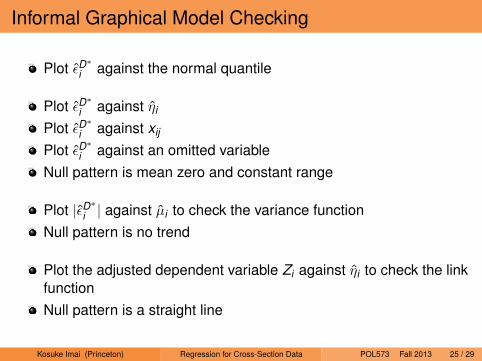
Informal Graphical Model Checking
Plot εD∗
i against the normal quantile
Plot εD∗
i against ηi
Plot εD∗
i against xij
Plot εD∗
i against an omitted variableNull pattern is mean zero and constant range
Plot |εD∗i | against µi to check the variance functionNull pattern is no trend
Plot the adjusted dependent variable Zi against ηi to check the linkfunctionNull pattern is a straight line
Kosuke Imai (Princeton) Regression for Cross-Section Data POL573 Fall 2013 25 / 29
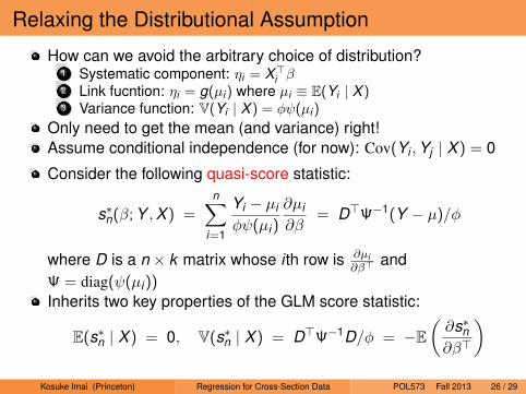
Relaxing the Distributional Assumption
How can we avoid the arbitrary choice of distribution?1 Systematic component: ηi = X>
i β2 Link fucntion: ηi = g(µi ) where µi ≡ E(Yi | X )3 Variance function: V(Yi | X ) = φψ(µi )
Only need to get the mean (and variance) right!Assume conditional independence (for now): Cov(Yi ,Yj | X ) = 0
Consider the following quasi-score statistic:
s∗n(β; Y ,X ) =n∑
i=1
Yi − µi
φψ(µi)
∂µi
∂β= D>Ψ−1(Y − µ)/φ
where D is a n × k matrix whose i th row is ∂µi∂β>
andΨ = diag(ψ(µi))Inherits two key properties of the GLM score statistic:
E(s∗n | X ) = 0, V(s∗n | X ) = D>Ψ−1D/φ = −E(∂s∗n∂β>
)Kosuke Imai (Princeton) Regression for Cross-Section Data POL573 Fall 2013 26 / 29
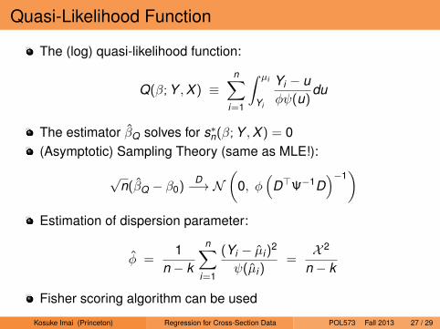
Quasi-Likelihood Function
The (log) quasi-likelihood function:
Q(β; Y ,X ) ≡n∑
i=1
∫ µi
Yi
Yi − uφψ(u)
du
The estimator βQ solves for s∗n(β; Y ,X ) = 0(Asymptotic) Sampling Theory (same as MLE!):
√n(βQ − β0)
D−→ N(
0, φ(
D>Ψ−1D)−1
)Estimation of dispersion parameter:
φ =1
n − k
n∑i=1
(Yi − µi)2
ψ(µi)=X 2
n − k
Fisher scoring algorithm can be used
Kosuke Imai (Princeton) Regression for Cross-Section Data POL573 Fall 2013 27 / 29
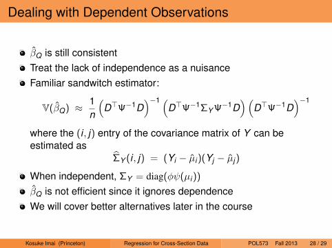
Dealing with Dependent Observations
βQ is still consistentTreat the lack of independence as a nuisanceFamiliar sandwitch estimator:
V(βQ) ≈ 1n
(D>Ψ−1D
)−1 (D>Ψ−1ΣY Ψ−1D
)(D>Ψ−1D
)−1
where the (i , j) entry of the covariance matrix of Y can beestimated as
ΣY (i , j) = (Yi − µi)(Yj − µj)
When independent, ΣY = diag(φψ(µi))
βQ is not efficient since it ignores dependenceWe will cover better alternatives later in the course
Kosuke Imai (Princeton) Regression for Cross-Section Data POL573 Fall 2013 28 / 29
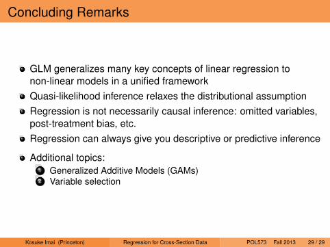
Concluding Remarks
GLM generalizes many key concepts of linear regression tonon-linear models in a unified frameworkQuasi-likelihood inference relaxes the distributional assumptionRegression is not necessarily causal inference: omitted variables,post-treatment bias, etc.Regression can always give you descriptive or predictive inference
Additional topics:1 Generalized Additive Models (GAMs)2 Variable selection
Kosuke Imai (Princeton) Regression for Cross-Section Data POL573 Fall 2013 29 / 29


![Applied Nonparametric Regression [Hardle]](https://img.dokumen.tips/doc/110x75/551eb84d497959cf398b4b76/applied-nonparametric-regression-hardle.jpg)

![(eBook-PDF) - Statistics - Applied Nonparametric Regression[1]](https://img.dokumen.tips/doc/110x75/55cf99ab550346d0339e92b5/ebook-pdf-statistics-applied-nonparametric-regression1.jpg)


![[Bruderl] Applied Regression Analysis Using Stata](https://img.dokumen.tips/doc/110x75/55cf96a7550346d0338ce88d/bruderl-applied-regression-analysis-using-stata.jpg)


