STATISTICS 3AO3

Applied Regression Analysis with SAS

Angelo J. Canty

Office : Hamilton Hall 209

Phone : (905) 525-9140 extn 27079

E-mail : cantya@mcmaster.ca

Lab (Mandatory) : Tuesday, 5:30pm in BSB-244.

Office Hours : Monday, Thursday 9:30-10:20or at other times by e-mail appointment.

Website : All lecture notes and announcements about the coursewill be made on the websitehttp://www.math.mcmaster.ca/canty/teaching/stat3a03

Required Text : Regression Analysis By Example (Fourth Edi-tion) Samprit Chatterjee & Ali S. Hadi. Wiley (2006)

Optional (recommended) Text : Applied Linear Regression (ThirdEdition) Sanford Weisberg. Wiley (2005)

1

Background Review

Some Definitions

1. A Random Experiment is an experiment which can be re-peated under the same conditions but whose outcome cannotbe predicted with certainty.

2. The set of all possible outcomes of a random experiment iscalled the Sample Space.

3. An Event is a set of possible outcomes of a random experi-ment — a subset of the sample space.

4. A Random Variable is a function mapping the Sample Spaceto a set of numbers.

2

Random Variables

∗ Random variables are denoted using upper case letters X,Y, . . ..

∗ The observed values of a random variable are denoted by lower

case letters x, y, . . ..

∗ Every random variable has a corresponding distribution which

describes how its values varies over repeated random exper-

iments.

∗ In this course we will primarily be dealing with continuous

random variables which can take values on the whole real

line or an interval on the real line.

3

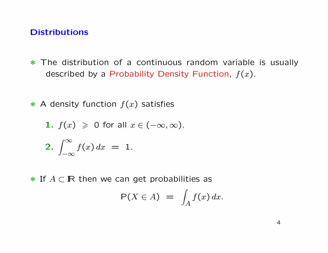
Distributions

∗ The distribution of a continuous random variable is usually

described by a Probability Density Function, f(x).

∗ A density function f(x) satisfies

1. f(x) > 0 for all x ∈ (−∞,∞).

2.∫ ∞−∞

f(x) dx = 1.

∗ If A ⊂ IR then we can get probabilities as

P(X ∈ A) =∫Af(x) dx.

4

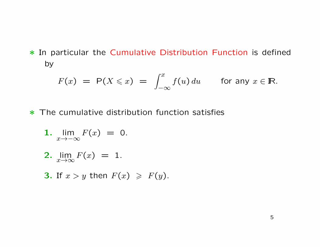
∗ In particular the Cumulative Distribution Function is defined

by

F (x) = P(X 6 x) =∫ x

−∞f(u) du for any x ∈ IR.

∗ The cumulative distribution function satisfies

1. limx→−∞

F (x) = 0.

2. limx→∞F (x) = 1.

3. If x > y then F (x) > F (y).

5

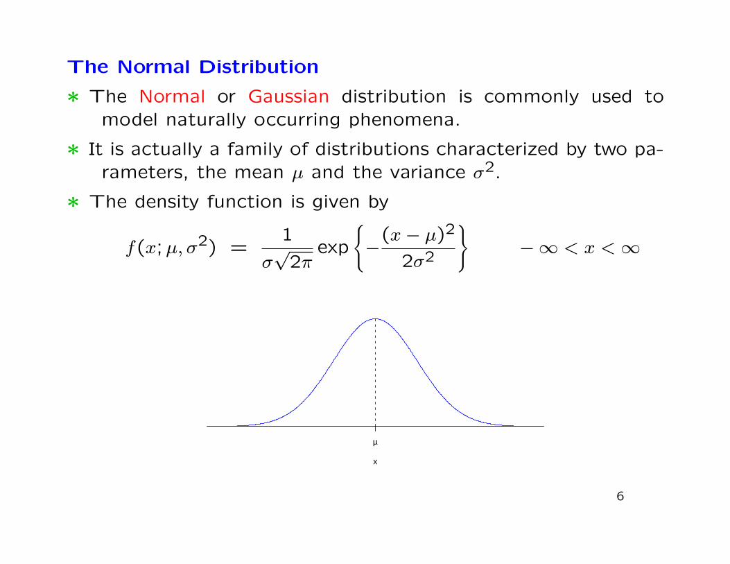
The Normal Distribution

∗ The Normal or Gaussian distribution is commonly used tomodel naturally occurring phenomena.

∗ It is actually a family of distributions characterized by two pa-rameters, the mean µ and the variance σ2.

∗ The density function is given by

f(x;µ, σ2) =1

σ√

2πexp

{−

(x− µ)2

2σ2

}−∞ < x <∞

x

µ

6

The Standard Normal Distribution

∗ A normal random variable with µ = 0 and σ = 1 is called a

Standard Normal random variable.

∗ Standard normal random variables are traditionally denoted Z.

∗ If Z ∼ N(0,1) then X = µ+ σZ ∼ N(µ, σ2).

∗ Conversely if X ∼ N(µ, σ2) then

Z =X − µσ

∼ N(0,1)

7

Random Vectors

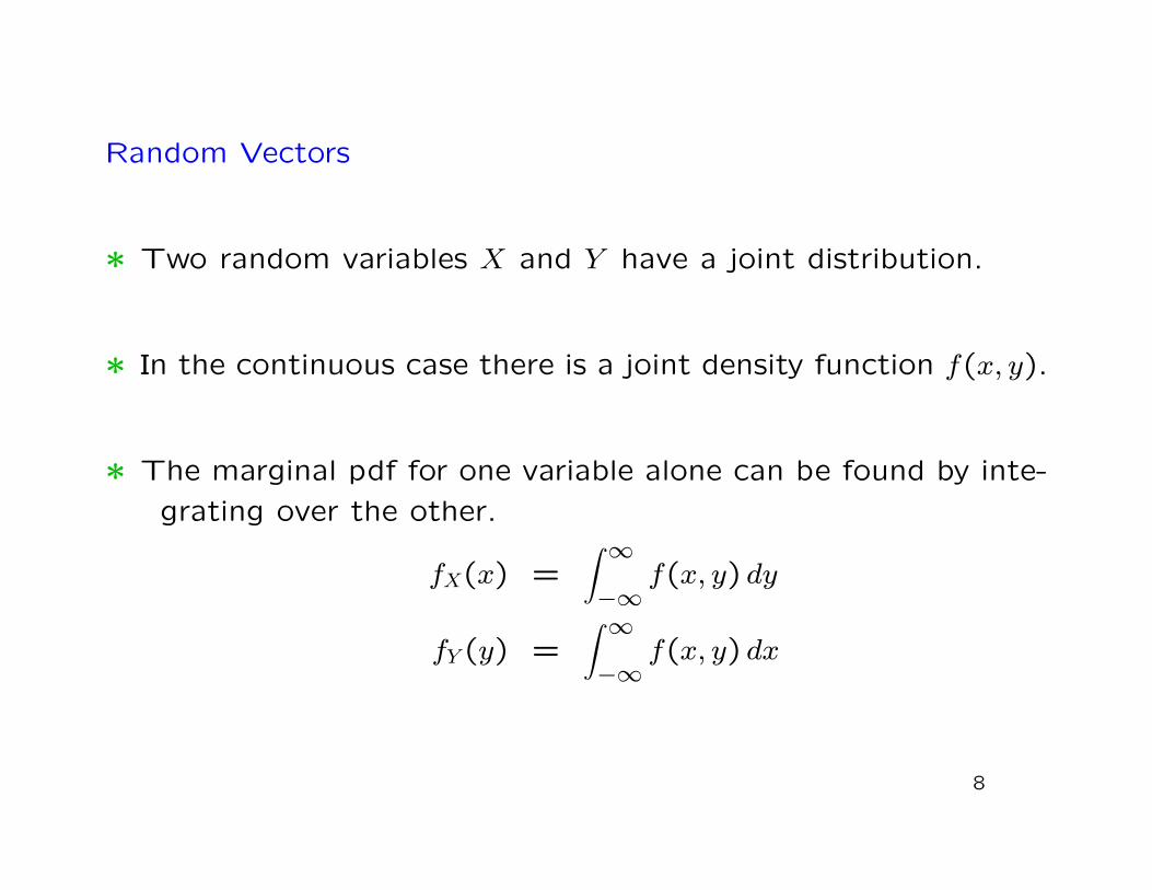
∗ Two random variables X and Y have a joint distribution.

∗ In the continuous case there is a joint density function f(x, y).

∗ The marginal pdf for one variable alone can be found by inte-

grating over the other.

fX(x) =∫ ∞−∞

f(x, y) dy

fY (y) =∫ ∞−∞

f(x, y) dx

8

Conditional Distributions

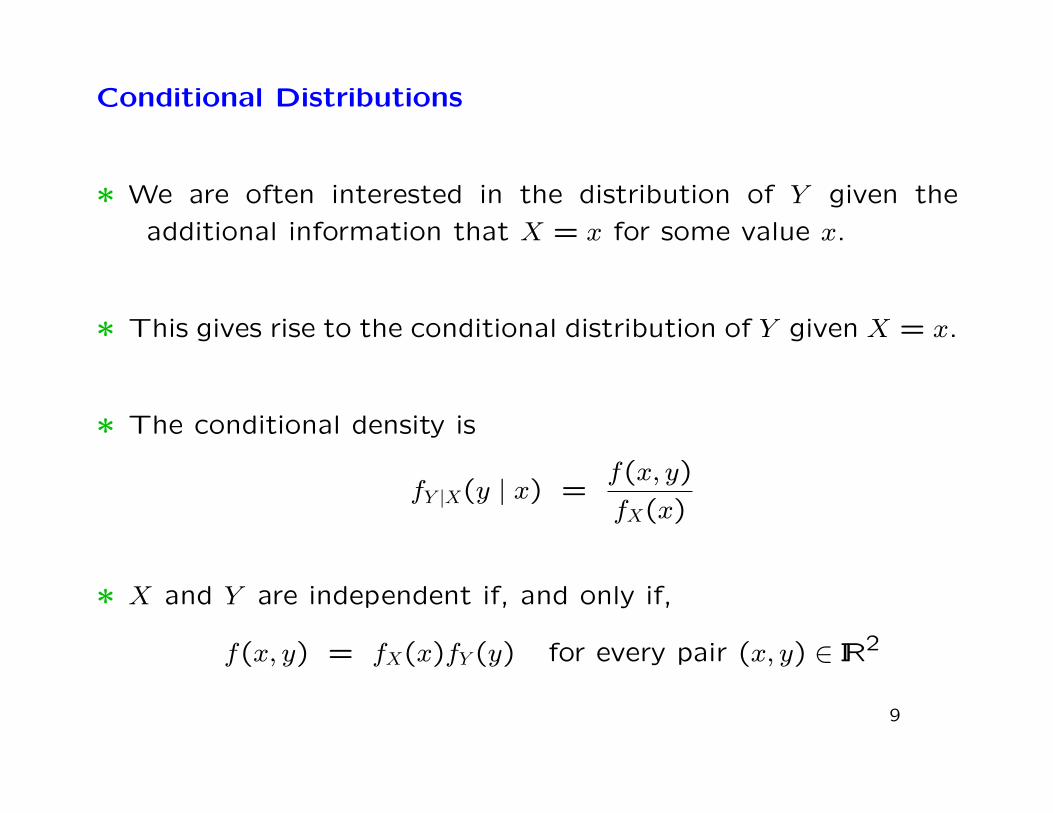
∗ We are often interested in the distribution of Y given the

additional information that X = x for some value x.

∗ This gives rise to the conditional distribution of Y given X = x.

∗ The conditional density is

fY |X(y | x) =f(x, y)

fX(x)

∗ X and Y are independent if, and only if,

f(x, y) = fX(x)fY (y) for every pair (x, y) ∈ IR2

9

Random Samples

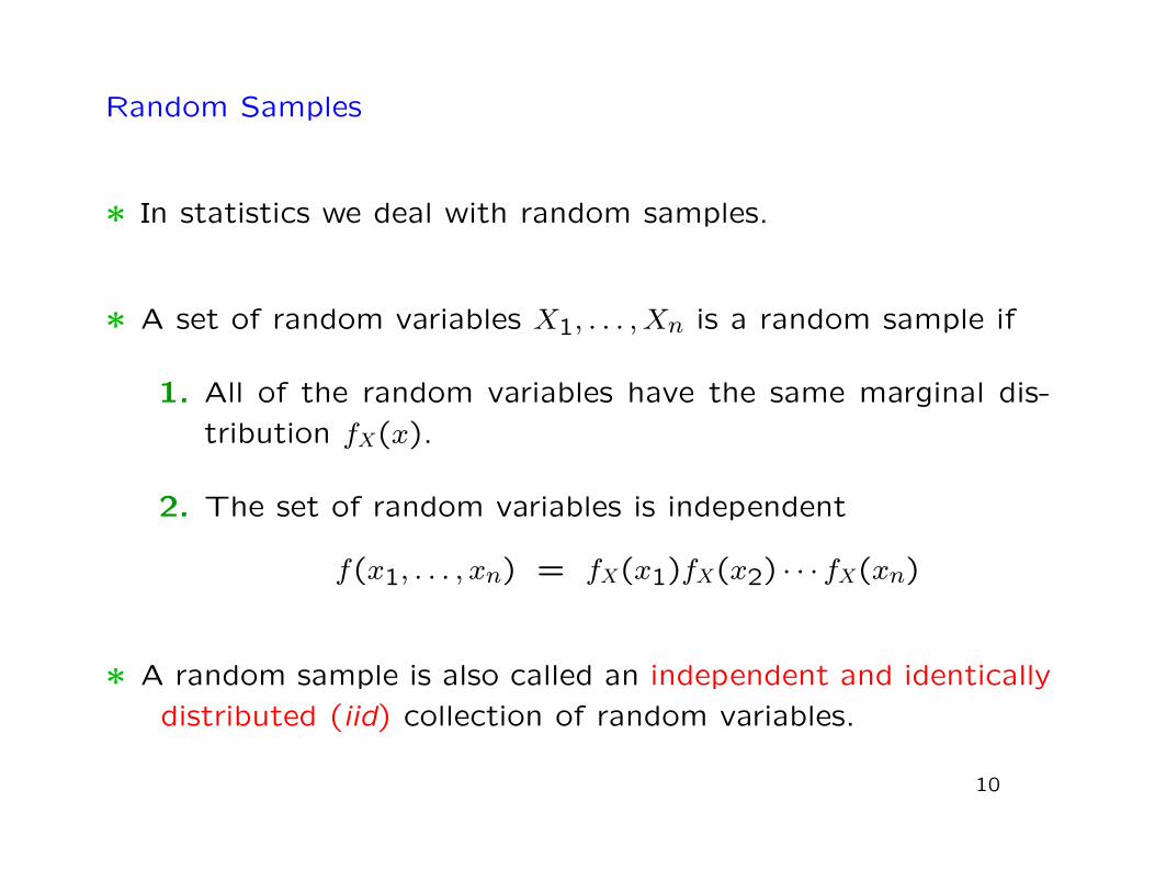
∗ In statistics we deal with random samples.

∗ A set of random variables X1, . . . , Xn is a random sample if

1. All of the random variables have the same marginal dis-

tribution fX(x).

2. The set of random variables is independent

f(x1, . . . , xn) = fX(x1)fX(x2) · · · fX(xn)

∗ A random sample is also called an independent and identically

distributed (iid) collection of random variables.

10

Statistical Inference

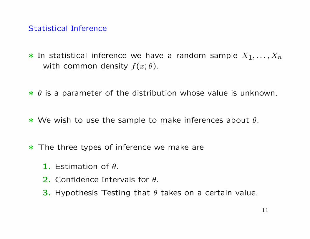
∗ In statistical inference we have a random sample X1, . . . , Xnwith common density f(x; θ).

∗ θ is a parameter of the distribution whose value is unknown.

∗ We wish to use the sample to make inferences about θ.

∗ The three types of inference we make are

1. Estimation of θ.

2. Confidence Intervals for θ.

3. Hypothesis Testing that θ takes on a certain value.

11

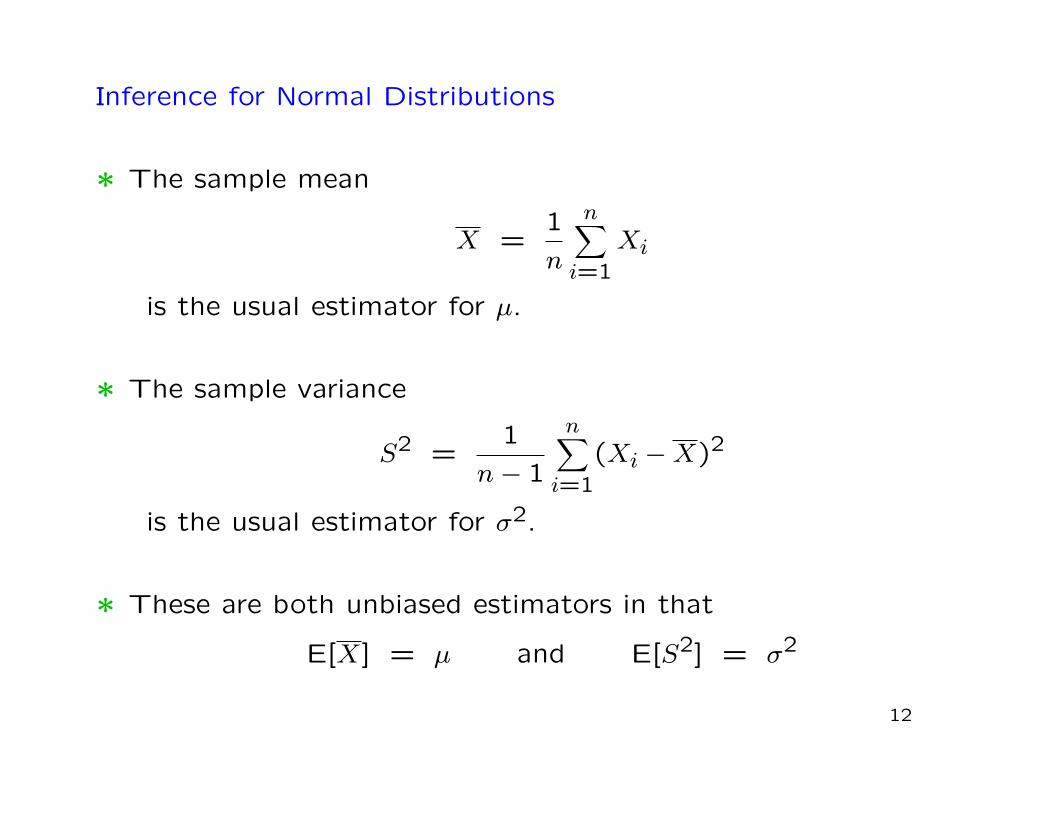
Inference for Normal Distributions

∗ The sample mean

X =1

n

n∑i=1

Xi

is the usual estimator for µ.

∗ The sample variance

S2 =1

n− 1

n∑i=1

(Xi −X)2

is the usual estimator for σ2.

∗ These are both unbiased estimators in that

E[X] = µ and E[S2] = σ2

12

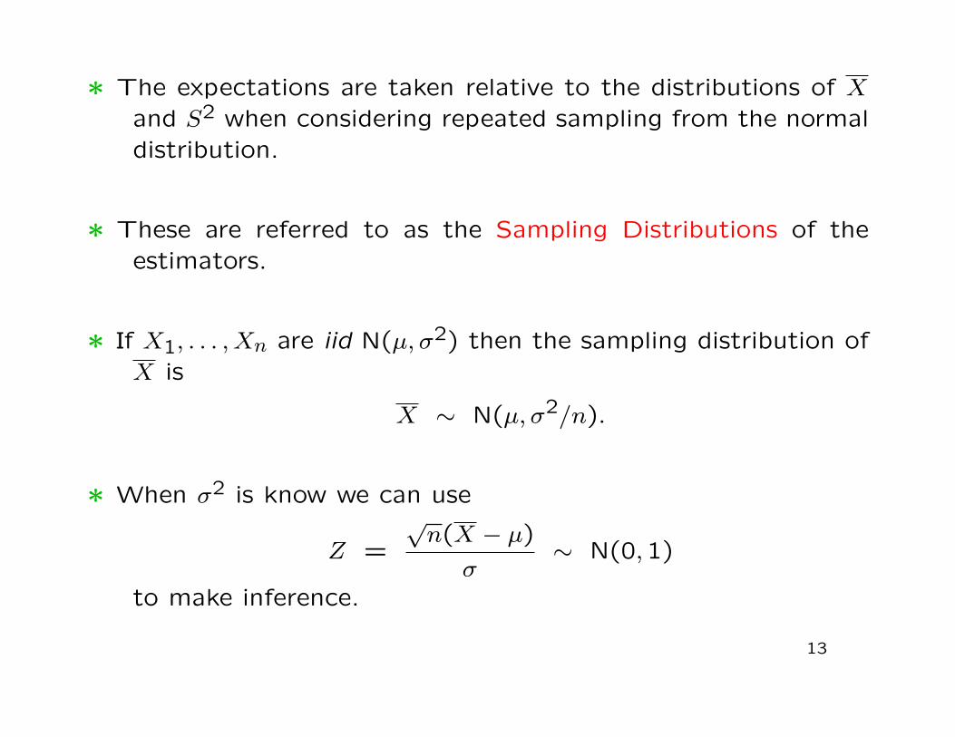
∗ The expectations are taken relative to the distributions of Xand S2 when considering repeated sampling from the normaldistribution.

∗ These are referred to as the Sampling Distributions of theestimators.

∗ If X1, . . . , Xn are iid N(µ, σ2) then the sampling distribution ofX is

X ∼ N(µ, σ2/n).

∗ When σ2 is know we can use

Z =

√n(X − µ)

σ∼ N(0,1)

to make inference.

13

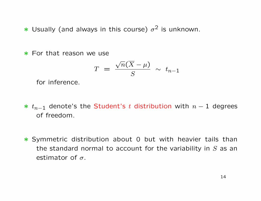
∗ Usually (and always in this course) σ2 is unknown.

∗ For that reason we use

T =

√n(X − µ)

S∼ tn−1

for inference.

∗ tn−1 denote’s the Student’s t distribution with n − 1 degrees

of freedom.

∗ Symmetric distribution about 0 but with heavier tails than

the standard normal to account for the variability in S as an

estimator of σ.

14

Introduction to Regression

∗ The aim of regression is to model the dependence of one

variable Y on a set of variables X1, . . . , Xp.

∗ Y is called the dependent variable or the response variable.

∗ X1, . . . , Xp are called the independent variables or covariates.

∗ For the majority of this course, Y will be a continuous or

quantitative variable.

15

∗ When all of the covariates are continuous we are dealing with

what is classically called regression.

∗ When all of the covariates are discrete, we are dealing with

Analysis of Variance (ANOVA).

∗ When some covariates are discrete and some are continuous

the term Analysis of Covariance (ANCOVA) is often used.

∗ We shall see that all of these can be easily expressed using the

linear model framework.

16

The General Regression Model

∗ A general model for predicting Y given the covariates X1, . . . , Xpwould be

Y = f(X1, . . . , Xp) + ε

∗ The term ε is usually called the Random Error and explains

the variability of the random variable Y about f(X1, . . . , Xp).

∗ The function f is a totally deterministic function whose form

is decided on by the analyst.

∗ Generally the function will also depend on a set of unknown

parameters β0, . . . , βp.

17

The Linear Regression Model

∗ For the most part we will deal with the situation where theparameters enter the function f in a linear way.

∗ This results in the linear model

Y = β0 + β1X1 + β2X2 + · · ·+ βpXp + ε

∗ Furthermore we will generally assume that the random errorε is normally distributed with mean 0 and unknown varianceσ2 for any values of the covariates.

∗ The aim of regression is then to make inferences about thep+ 2 unknown parameters in this model.

18

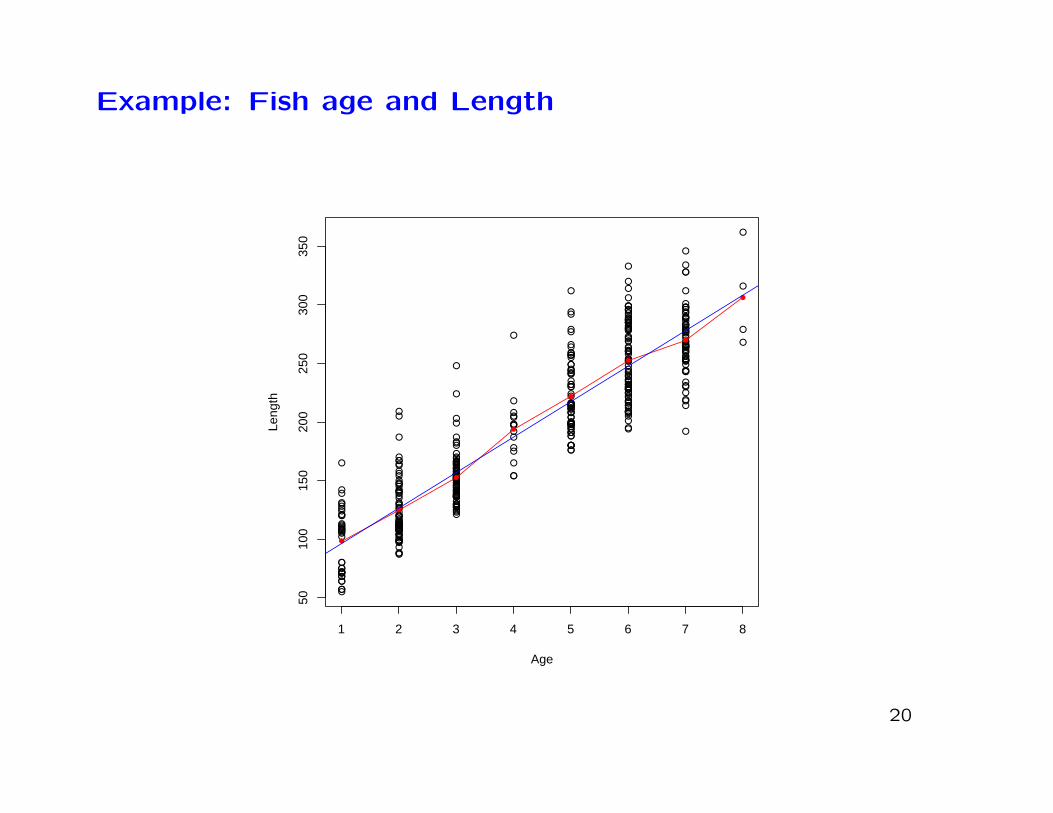
Example: Fish age and Length

∗ The growth pattern of game fish, such as the smallmouthbass, is of interest to agencies who manage stocks in inlandlakes.

∗ In this example 439 smallmouth bass, of at least one year old,were caught in West Bearskin Lake in Minnesota.

∗ For each fish, their age was measured using annular rings ontheir scales. Their length was also measured.

∗ We wish to fit the model

Length = β0 + β1Age + ε

19

Example: Fish age and Length

●●●

●●●

●

●

●●●●●●●●●●●●●●●

●

●

●

●

●

●

●

●

●

●●

●

●

●●

●

●

●●

●

●

●

●●●

●●

●

●●

●●●

●

●

●●

●●

●

●

●

●

●

●●

●

●

●

●

●

●

●

●

●

●

●

●

●

●

●

●●

● ●

●

●●

●

●

●●●

●●●●●●●

●●●●

●●●●●

●●

●●●●

●

●

●●●●●●●●●●●●●●●●●●●●●●●●●●●●●

●●●

●

●●

●●●●●●●●●●●●●●●●●●●●●●●●●●●

●●●●●●●●●

●●●

●●●●●

●

●●● ●

●

●

●

●●

●●●

●●

●●●●●

●

●

●

●●

●

●

●

●●

●

●●●

●●

●●

●

●●

●

●●

●●

●●●

●●●●●

●●●●●●

●●●●●●

●

●

●

●●

●

●

●●

●

●

●

●●●●●●●●●●●●●●●●

●

●

● ●

●

●

●

●

●●

●●

●

●

●

●

●

●

●●

●●

●

●

●●

●●●

●

●

●

●

●

●

●

●

●

●●●

●

●

●

●

●

●●●●●●●

●●●●●

●●●

●

●●●●

●●●●●

●●●

●●●

●

●

●

●

●

●

●

●

●

●

●

●

●

●●●

●

●

●●

●●●●●●●●●

●

●

●●●

●

●

●●●●●●

●

●●

●●●●●●

●●●

●

●●●

●●●●

●

●

●

●

●

●

●

1 2 3 4 5 6 7 8

5010

015

020

025

030

035

0

Age

Leng

th

●

●

●

●

●

●

●

●

20

Example: Fish age and Length

∗ The red dots are the mean lengths examining only fish of agiven age.

∗ The blue line is the fitted regression line

Length = 65.53 + 30.32×Age

∗ The blue line seems to follow the mean ages very well.

∗ Individual fish, however, vary about this line quite a bit.

∗ The fitted line tells us that, on average, fish grow 30.32mmper year after 1 year of age.

21

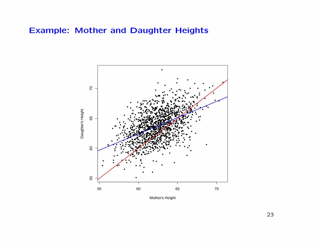
Example: Mother and Daughter Heights

∗ How does a mother’s height affect her daughter’s height?

∗ We would expect tall mothers to have tall daughters and shortmothers to have short daughters.

∗ Do daughters tend to be the same height as their mother, onaverage?

∗ To answer this question, the famous statistician Karl Pearsonrecorded the heights of 1375 British mothers and their adultdaughters in the period 1893–1898.

∗ The data were published in 1903 in one of the first publicationsto look at heredity of physical traits using real data.

22

Example: Mother and Daughter Heights

●

●

●

●

●

●

●

●

●●

●

●

●●

●

● ●●

●

●

●

●

●

●

●●

●

●●

●

●●

●

●

●

●

●●

●●● ●

●

●●

●

●

●

●

●●

●

●

●●

●

● ●

●●

●

●●

●

●●

●●

●

●

●●●

●

●

●

●●

●

●

●

●

●

●● ●

●

●

●●

●

●●

●●

●

●

●●

●●

●

●

●

●

●

●●

●●

●●

●

●

●

●

●●

●

●

●● ●

●

●

●●

●●

●●

●●

●●

●●

●

●●

●

●

●●●

●●

●●●●

●

●

●

●●

●

●

●●

●

●●●

●

●

●

● ●

●

●●

●●

●

●●

●

●●

●●

●

●

●

●

●

●

●●

●●

●●

●

●

●●

●

●

●

●●

●

●

●

●

●

●

●●

●

●

●

●

●

●●

●

●●●

●●

●

●●

●

●

●

●●

●

●●

●

●

●

●

●●

●

●●

●

●●

●

●●

●

●●●

●●

●

●

●

●

●●

●●

●●

●

●●

●●

●

●●

●●

●

●

●

●

●●

●

●●

●

●

●

●●●

●

●●

●●

●

●

●

●●

●

●●

●●

●

●

●

●●

●●

●●

●●

●

●●●

●

●

●● ●

●

●

●

●

●

●

●●

●

●●

●●

●

●

●

● ●●

●

●

●●

●

●●

●

●●

●

●

●●

●●●

●●

●

●●

●

●

●● ● ●●

●●

●

●● ●●

●

●

●

●

●●

●●

●

●

●

●

●●

●●

●●

●

●●

●

●

●●

●

●

●●●

●●

●

●●

●●

●

● ●●

●●

●

●

●●●

●●

●

●●

●●

●●

●

●

●

●●

●

●

●

●

●

●

●

●●

●●

●●

●

●

●

●●

●

●●

●●

●●●

●

●

●●

●

●

● ●●

●●

●●

●●

● ●●

●

● ●

● ●

●

●●

●● ●

●●●

●●

●

●

●

●

●●

●●

●●

●

●

●

●●●

●

●

●●

●

●

●

●

●

●●

●

●

●

●●

●

●

●

●

●●

●●

●●

●●

●

●

●

●

●

●●

●

●

●

●●

●

●●●

●●

●

●

● ●

●

●

●

●

●

●

●●

●●

●●

●●

●●●

●●

●●

● ●

●●

●

●●

●●

●

●

●●

●●

●

●

●

●

●

●

●●

●

●●

●

●

●●

●

●●

●●

●

●●

●

●

●●

●

●

●●●

●●

●

●●

●

●●

●●●

●

●

● ●●

●●

●

● ●

●●

●

●

●

●

●●

●

●

●

●

●

●

● ●

●● ● ●

●●

●●

●

●

●●

●●

●●

●●●

● ●

●●

●

●

●●

●●

●

●

●●

●

●●

●

●

●

●●

●

●●

●●

●

●

●●

●

●●

●

●●●

●●

●●

●●

●

●

●

●

●●

●

●●

●

●

●

●●

●●●

●●

●

●●

●

●

●

●●

●

●

●

●

●

●●

●●

●● ●

●

●

●

●

●

●●

●

●

●●●

●●

●● ●●

●

●

●●

●●●

●●

●●

●

●●●

●

●●

●

●

●●●

●

●

●●●

●

●

●

●

●●

●●

●●

●

●

●

●

●

●

●●●●

●

●

●

●

●

●●

●●●●

●●

●

●

●

●

●

●●

●

●

●

●

●

●

●

●●

●●

●

●

● ●

●●

●

● ●

●

●

●●

●

●

●●

●●

●

●●

●●

●

●●

●

●

●

●●

●

●

●●●

●●

●

●●

●

●●

●●

●●

●● ●

●●

●

●

●

●

●

●●●

●

●●

●

●

●

●

●

●

●●

●

●●

●●

●●

●●

●●

●●

●●

●●

●●

●●

●●

●● ●

●

●

●●

●

●

●●●

●

●

●

●

●●

●

●●

●

●

●●

●

●●

●

●

●

●

●●

●

●

●

●

●

● ●

● ●

●

●● ●

●

●●

●●

●●

●

●

●

●

●

●

●●

●●●

●

●●

●

● ●●

●●

●●

●

●

●●

●●

●●

●

●

●

●●

●●

●

●●

●●●

●●

●●

●●

●

●

●●

●

●

●

●

●

●

●●

●

●

●●

●

●

●

●

●

●●

●●

●

●●

●●●

●

●●

●

●●

●●

●

●●

● ●●

●

●●

●●

●

●

●●

●●

●●●

●●

●●

●

●●●

●

●● ●

●

●

●

●

●

●

●

●● ●

●●

●●

●●

●

●●

●

●●

●●

●●

●

●

●

●

●●

●

●

●●

●

●

●●

●

●●

●●

●

●

●

●●

●●

●

●

●●

●

●

●

●●

●●

●

●

●

●

●●●

●

●

●●

●

●●

●

●

●●

●

●

●

●● ●

●

●●

●●

●

●

●

●

●

●●

●

●

●

●●

● ●●

●

●

●

●●

●●

●

●

●

●

●

●

●

●

●

●

●

●

●●

●

●

●●

●

●●

●

●

●●●

●

●

● ●●

●●

●

●●

●

● ●

●

●

●

● ●●

●

●●●

●

●

●

●●

●

●●

●●●●

●

●

●

●

●●

●

●●

●●

●●

●●

●●

●●

●●

●

●●

●

●

●

●

●●

●

●

●

●●

●●

●

●●

● ●

●

●

●

●

●

●

●

●

●

●

●

●●

●

●

55 60 65 70

5560

6570

Mother's Height

Dau

ghte

r's H

eigh

t

23

Example: Mother and Daughter Heights

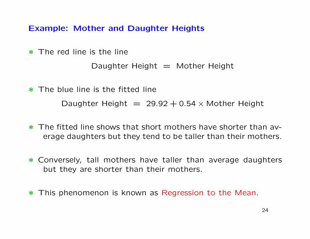
∗ The red line is the line

Daughter Height = Mother Height

∗ The blue line is the fitted line

Daughter Height = 29.92 + 0.54×Mother Height

∗ The fitted line shows that short mothers have shorter than av-erage daughters but they tend to be taller than their mothers.

∗ Conversely, tall mothers have taller than average daughtersbut they are shorter than their mothers.

∗ This phenomenon is known as Regression to the Mean.

24

The Regression Process

1. The researcher must clearly define the question(s) of interest

in the study.

2. The response variable Y must be decided on, based on the

question of interest.

3. A set of potentially relevant covariates, which can be mea-

sured, needs to be defined.

4. Data is collected.

25

Data Collection

∗ In some cases, called designed experiments the data can becollected in a controlled setting which will hold constant vari-ables which or not of interest.

∗ Controlled experiments also facilitate setting certain values ofthe covariates which are of interest to us.

∗ These types of experiments are common in areas such as in-dustrial process control, animal models for medical researchetc.

∗ In many studies, however, the data are collected by choos-ing a random sample of n individuals and observing Y andX1, . . . , Xp for those individuals.

26

Data Collection

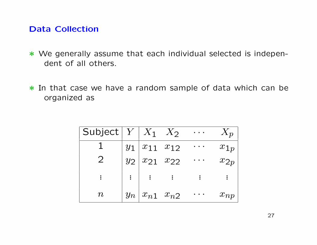
∗ We generally assume that each individual selected is indepen-dent of all others.

∗ In that case we have a random sample of data which can beorganized as

Subject Y X1 X2 · · · Xp

1 y1 x11 x12 · · · x1p

2 y2 x21 x22 · · · x2p

... ... ... ... ... ...

n yn xn1 xn2 · · · xnp

27

The Regression Process (continued)

5. Model Specification.

• What is the form of the model?

• What assumptions will we make?

6. Decide on a method for fitting the specified model.

7. Fit the model - typically using software such as SAS.

8. Examine the fitted model for violations of assumptions.

9. Conduct hypothesis testing for questions of interest.

10. Report the results from statistical inference.

28