Applied Economics for Business Management

Lecture outline:Introduction to courseMath reviewIntroduction to consumer behavior

Introduction

Applied economics for business management involves investigating both consumer and producer behavior. The course description states that the theory of the consumer, firm and market is developed. Often in agricultural economics programs, applied economics is covered in two courses – a course in applied production analysis and a course in applied price analysis. We will try to cover both topics in one course.

Introduction

The first half of the course will concentrate on consumer behavior and the second half of the course will be on producer behavior. But before we start on consumer behavior, we will do a quick math review. This will not be a review of calculus per se, but will provide an overview of optimization.

Math Review

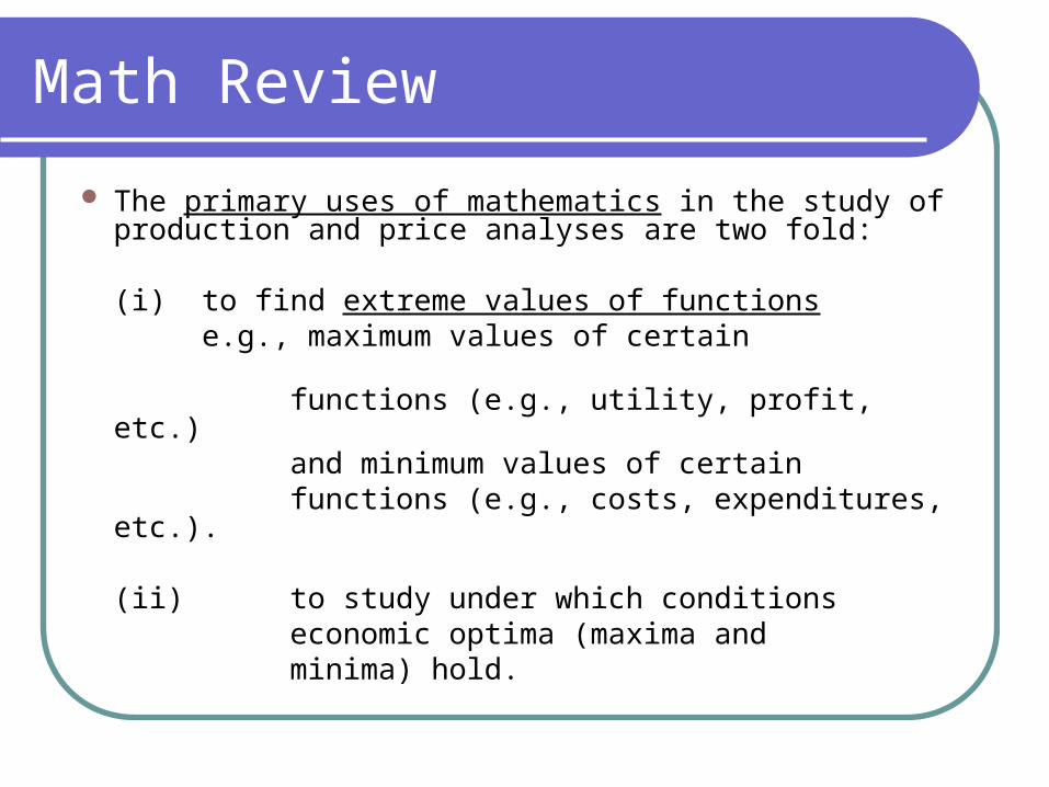
The primary uses of mathematics in the study of production and price analyses are two fold:(i) to find extreme values of functions e.g., maximum values of certain functions (e.g., utility, profit, etc.) and minimum values of certain functions (e.g., costs, expenditures, etc.).(ii) to study under which conditions economic optima (maxima and minima) hold.

Math Review

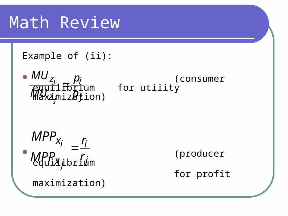
Example of (ii): (consumer equilibrium for utility maximization)

(producer equilibrium for profit maximization)

j

i

z

z

pp

MU

MU

j

i

j

i

x

x

MPP

MPP

j

irr

Math Review

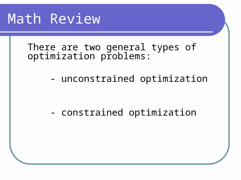
There are two general types of optimization problems: - unconstrained optimization - constrained optimization

Math Review

Unconstrained optimization(i) Simplest case: single argument functions with one explanatory variable(ii) General case:multiple argument functions

with n explanatory variables

Math Review

Suppose you had these two single argument functions:

Math Review

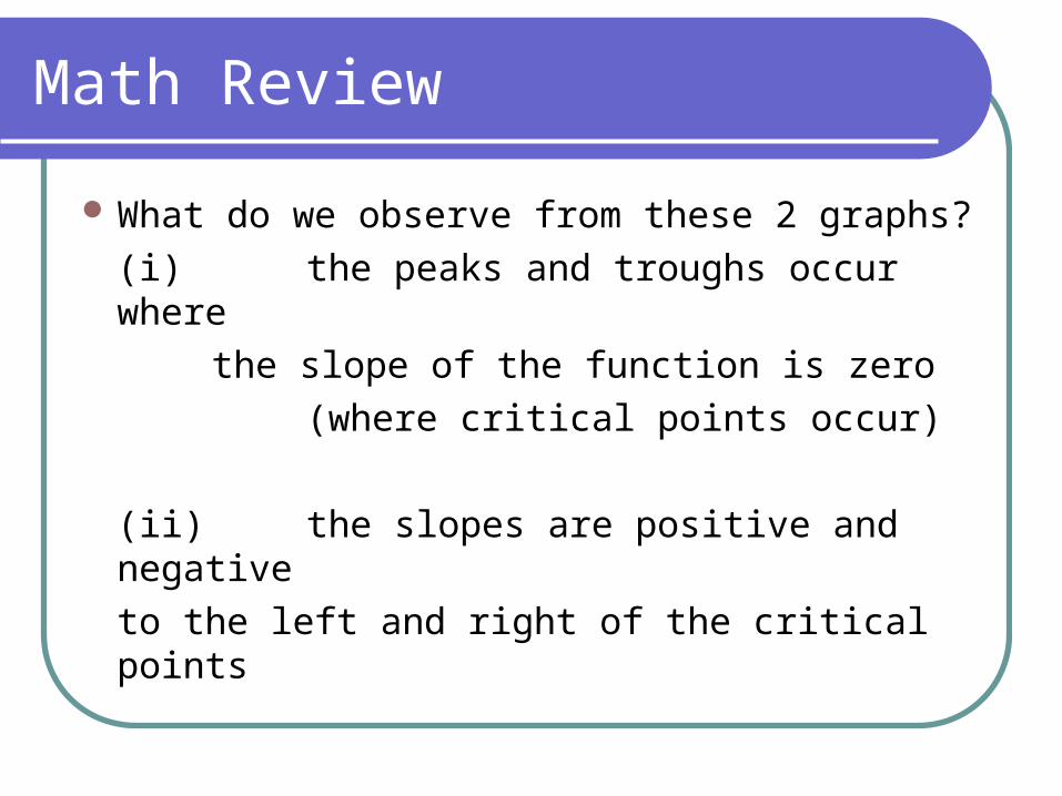
What do we observe from these 2 graphs?(i) the peaks and troughs occur where the slope of the function is zero (where critical points occur)(ii) the slopes are positive and negative

to the left and right of the critical points

Math Review

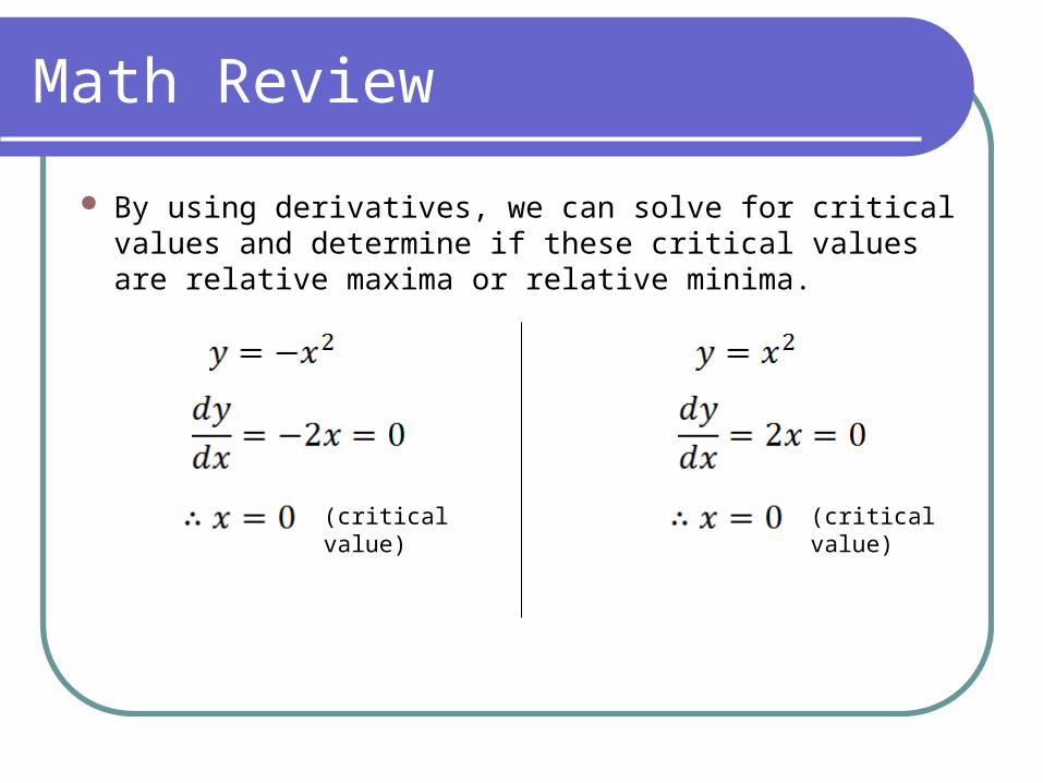
By using derivatives, we can solve for critical values and determine if these critical values are relative maxima or relative minima.

(critical value) (critical value)

Math Review

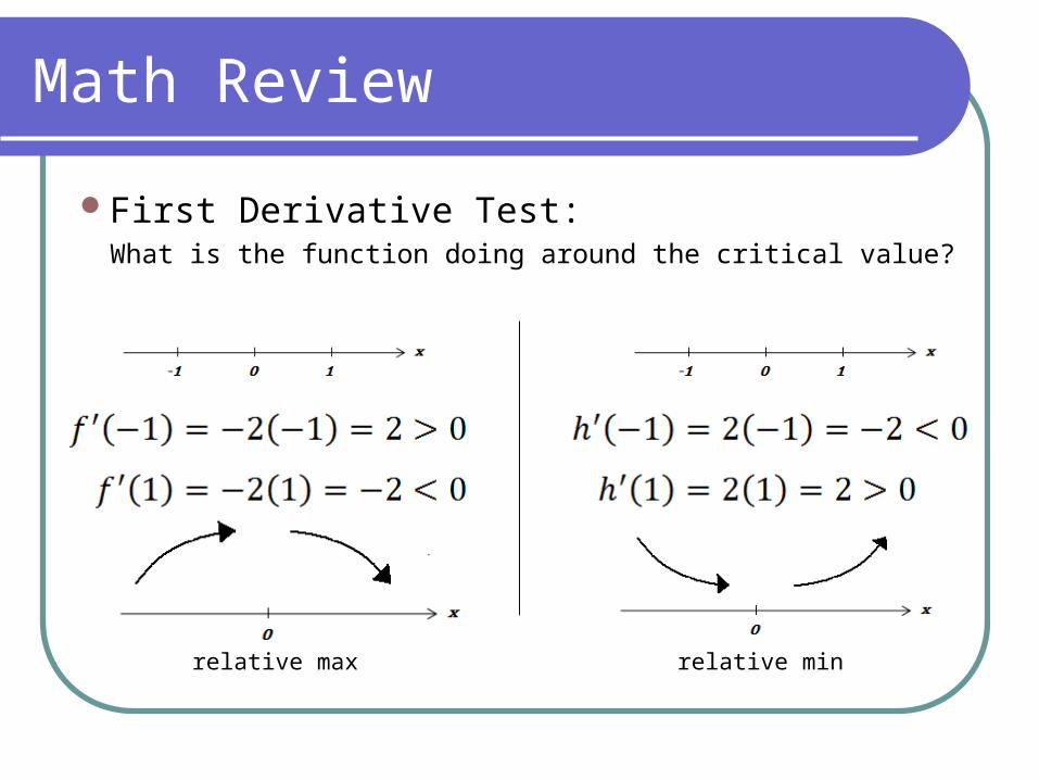
First Derivative Test:What is the function doing around the critical value?

relative max relative min

Math Review

Second Derivative Test:Another test to determine whether critical values are relative maximum(s)/minimum(s)(i) Relative maximum: second derivative is negative or concave down(ii) Relative minimum:second derivative is positive or concave up

Math Review

For the previous example: Critical value is a relative max

Critical value is a relative min

Math Review

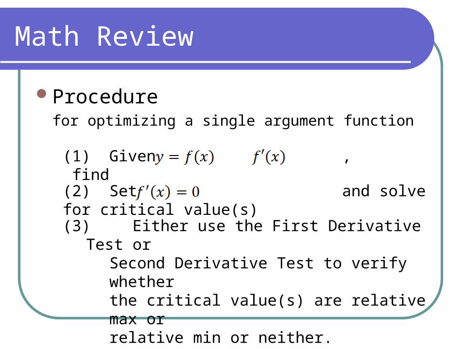
Procedurefor optimizing a single argument function(1) Given , find (2) Set and solve for critical value(s) (3) Either use the First Derivative Test or Second Derivative Test to verify whether the critical value(s) are relative max or relative min or neither.

Math Review

Example:Let

(critical value)

Math Review

Using the Second Derivative Test:is a relative min

Math Review

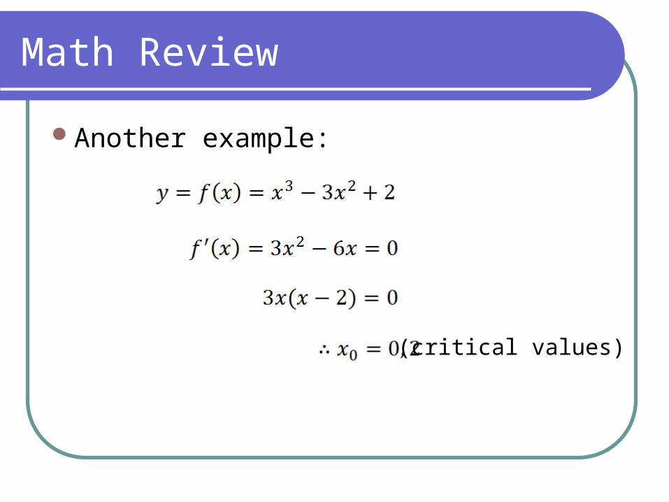
Another example:

(critical values)

Math Review

Second Derivative Test:is a relative maxis a relative min

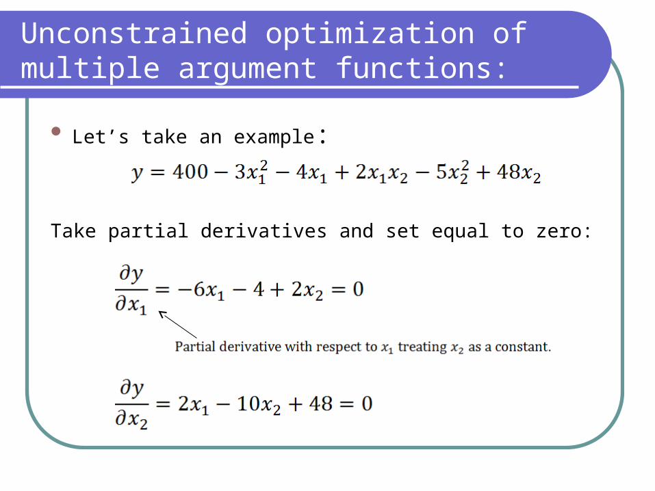
Unconstrained optimization of multiple argument functions:

Let’s take an example:Take partial derivatives and set equal to zero:

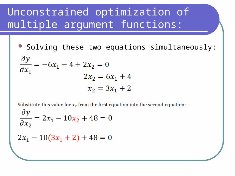
Unconstrained optimization of multiple argument functions:

Solving these two equations simultaneously:

Unconstrained optimization of multiple argument functions:

Distributing -10

Combining like terms

Subtracting -28 to both sides

Dividing both sides by -28

Unconstrained optimization of multiple argument functions:

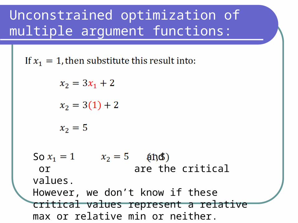
So and or are the critical values. However, we don’t know if these critical values represent a relative max or relative min or neither.

Math Review

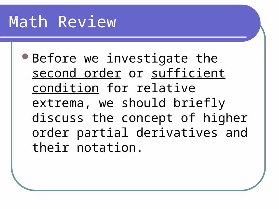
Before we investigate the second order or sufficient condition for relative extrema, we should briefly discuss the concept of higher order partial derivatives and their notation.

Math Review

GivenFirst order partial derivatives:

Math Review

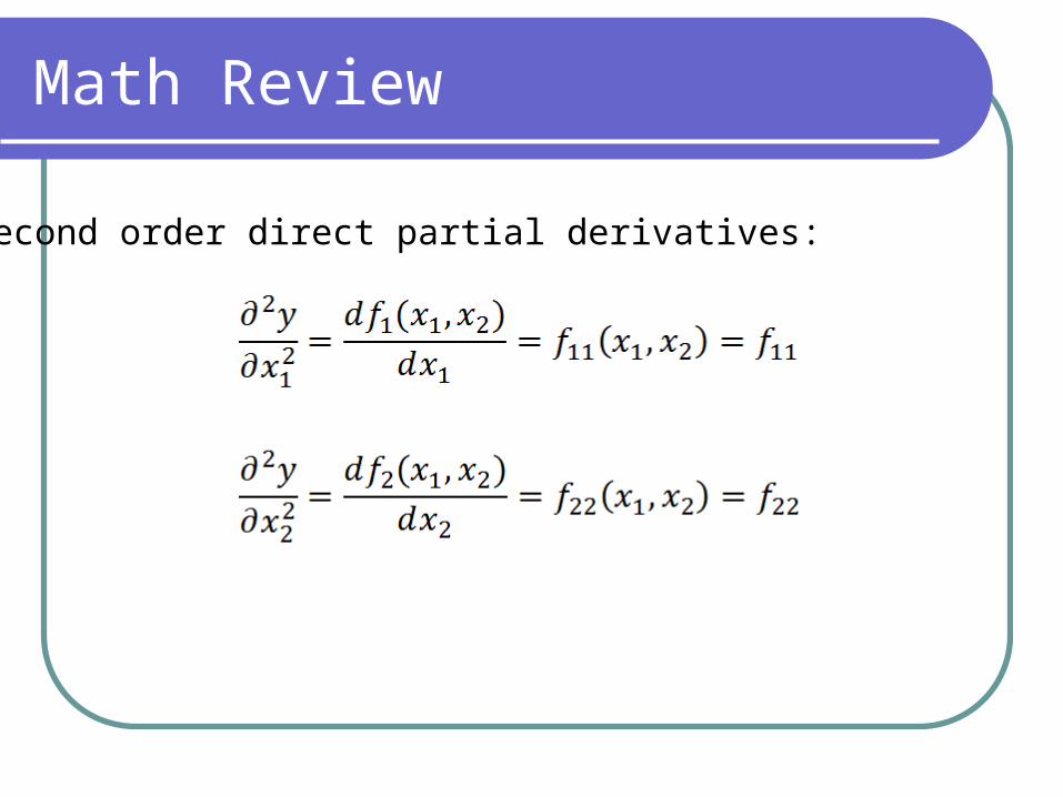
Second order direct partial derivatives:

Math Review

Second order cross partial derivatives:

If and are continuous functions, then by Young’s Theorem .See Silberberg (pages 68 – 70) for proof.

Unconstrained optimization of multiple argument functions:

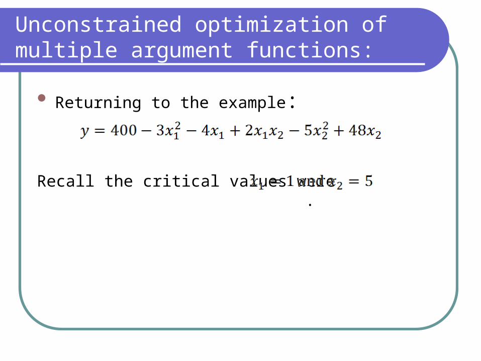
Returning to the example:Recall the critical values were .

Unconstrained optimization of multiple argument functions:

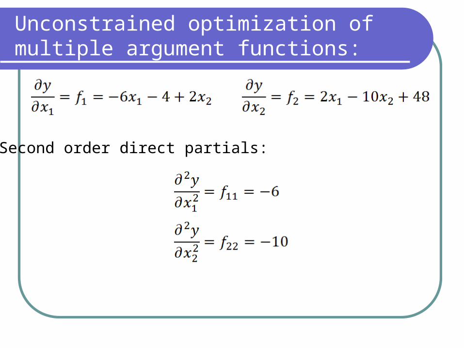
Also recall the following derivatives:

Unconstrained optimization of multiple argument functions:

Second order direct partials:

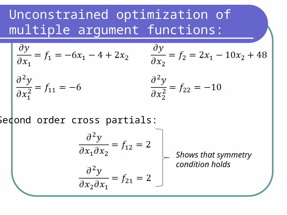
Unconstrained optimization of multiple argument functions:

Second order cross partials:Shows that symmetry condition holds

Unconstrained optimization of multiple argument functions:

Using the criteria for optimization with single argument functions, we are tempted to conclude that if and critical values represent a relative max Unfortunately, the second order conditions for multiple argument functions is not that simple. Because the sign of the second order direct partials only insure an extremum in the dimension or the dimension, but not the dimension.

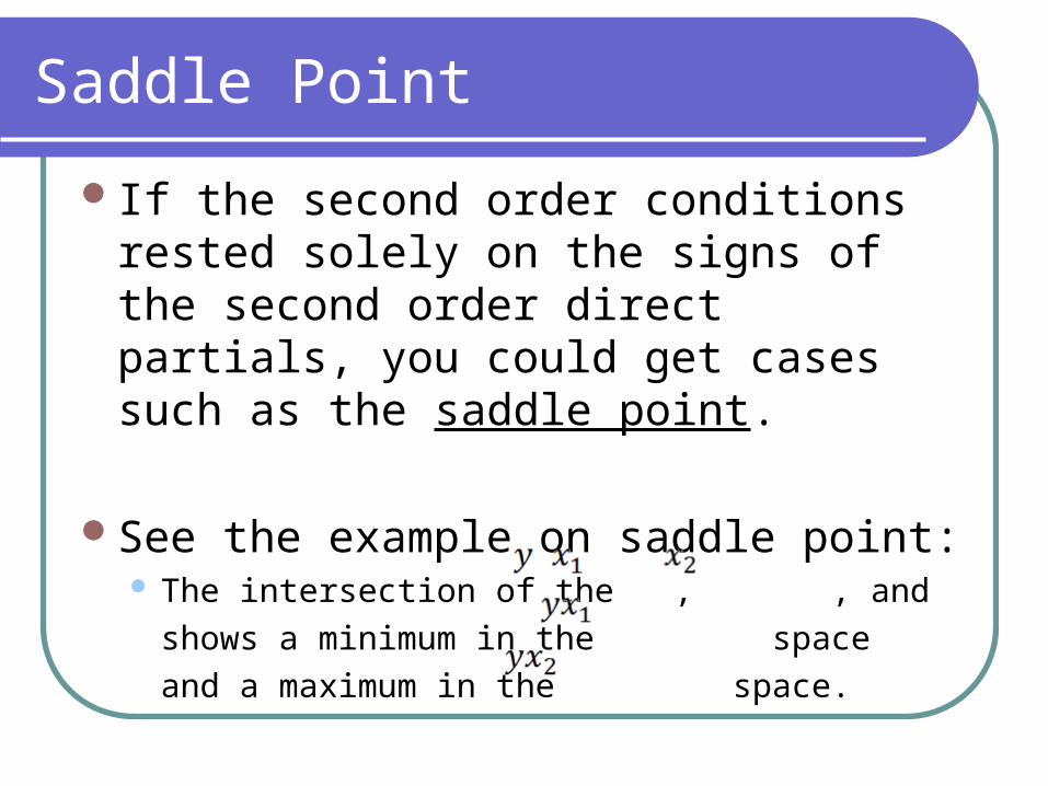
Saddle Point

If the second order conditions rested solely on the signs of the second order direct partials, you could get cases such as the saddle point.See the example on saddle point:

The intersection of the , , and shows a minimum in the space and a maximum in the space.

Saddle Point

The point being: the second order condition for multiple argument functions is not so simple.For this case, we have to set-up and then evaluate a Hessian determinant.

Where

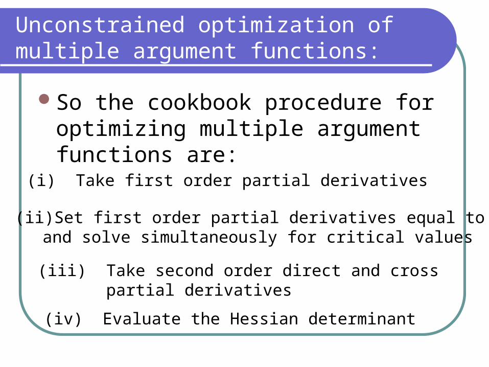
Unconstrained optimization of multiple argument functions:

So the cookbook procedure for optimizing multiple argument functions are:(i) Take first order partial derivatives(ii) Set first order partial derivatives equal to zeroand solve simultaneously for critical values(iii) Take second order direct and cross partial derivatives(iv) Evaluate the Hessian determinant

Determinants

Square matrix: Number of rows and columns are equal

Review of determinants: Associated with any square matrix A, there is a scalar quantity called the determinant of A and written: or |A| If A is n x n, then |A| is said to be of order n.(So n is the dimension of the square matrix)

Determinants

Determinants are defined as follows:

(1 x 1) matrix

Determinants

Determinants

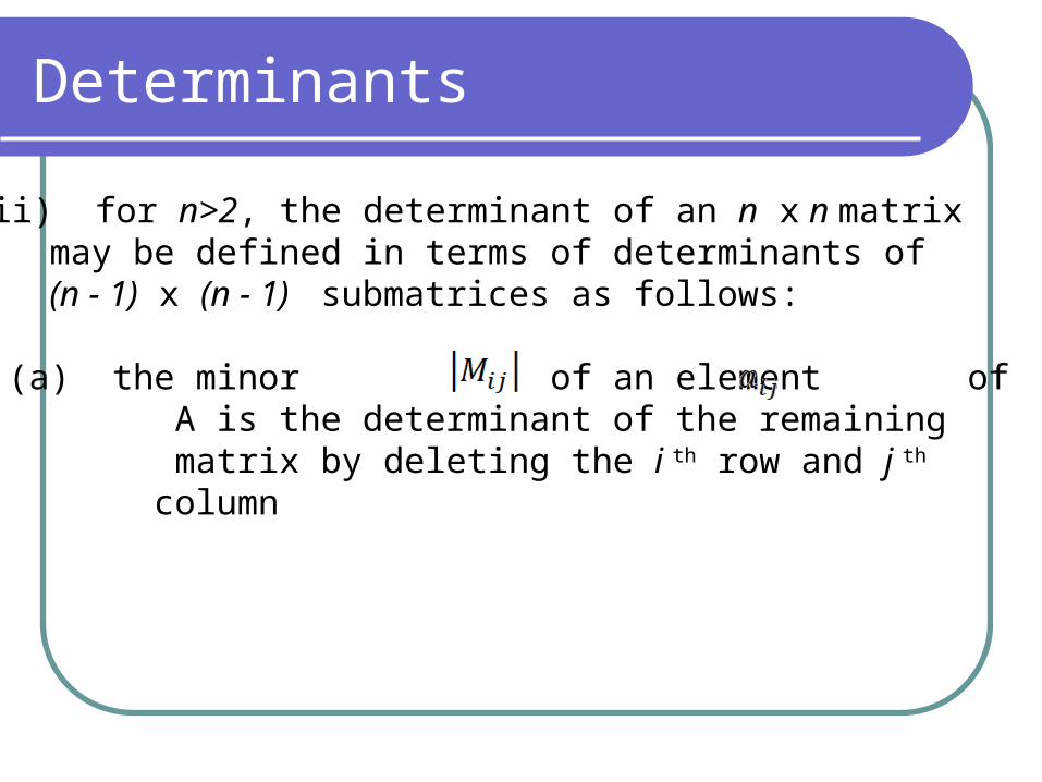
(iii) for n>2, the determinant of an n x n matrix may be defined in terms of determinants of (n - 1) x (n - 1) submatrices as follows:(a) the minor of an element of A is the determinant of the remaining matrix by deleting the i th row and j th column

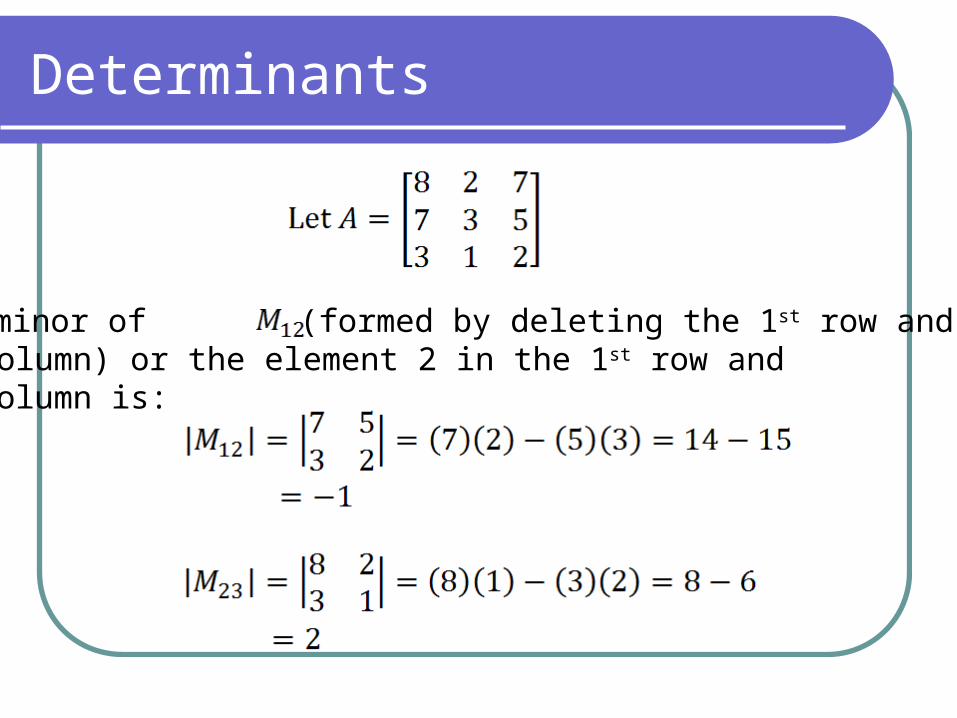
Determinants

The minor of (formed by deleting the 1st row and 2nd column) or the element 2 in the 1st row and 2nd column is:

Determinants

(b) Cofactor of is written in terms of its assigned minor.

Determinants

(c) The determinant of an n x n matrix is defined as the sum of the product of theelements of any row or column of A and their cofactors

Determinants

La Place Transformation by any row or any column.By any row:1st row2nd row3rd row

Determinants

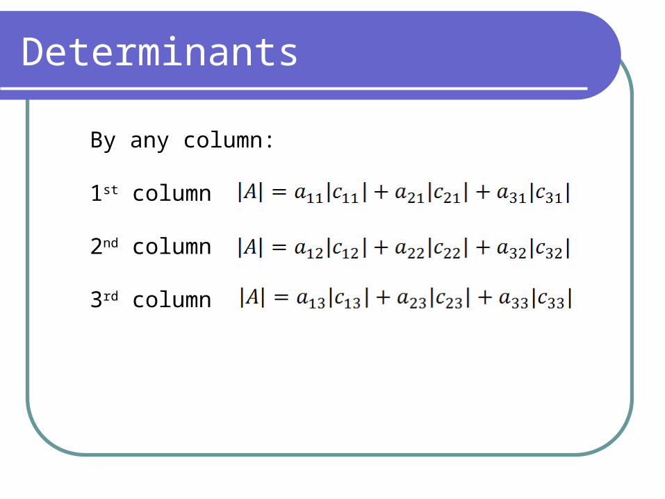
By any column:1st column2nd column3rd column

Determinants

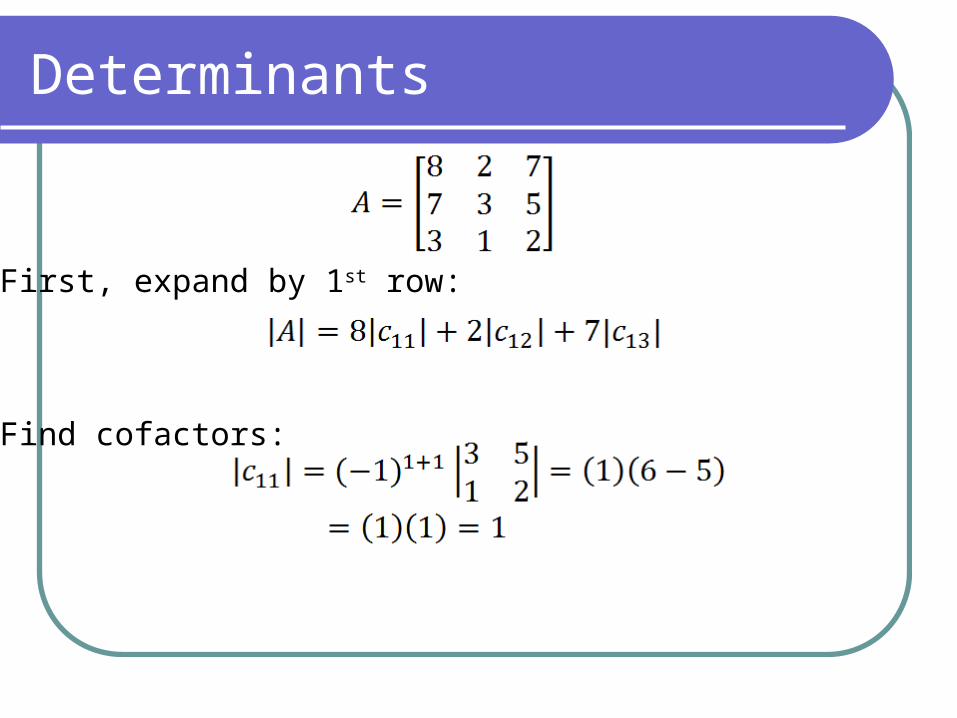
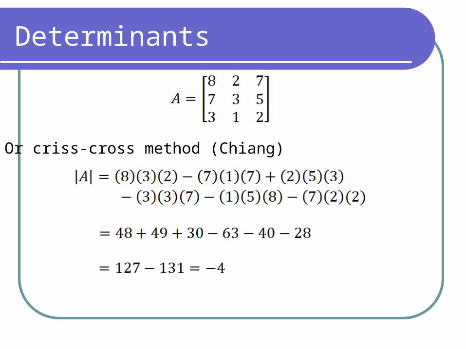
Find |A|.You can use the La Place Transformation by expanding on any row or column.

Determinants

First, expand by 1st row:Find cofactors:

Determinants

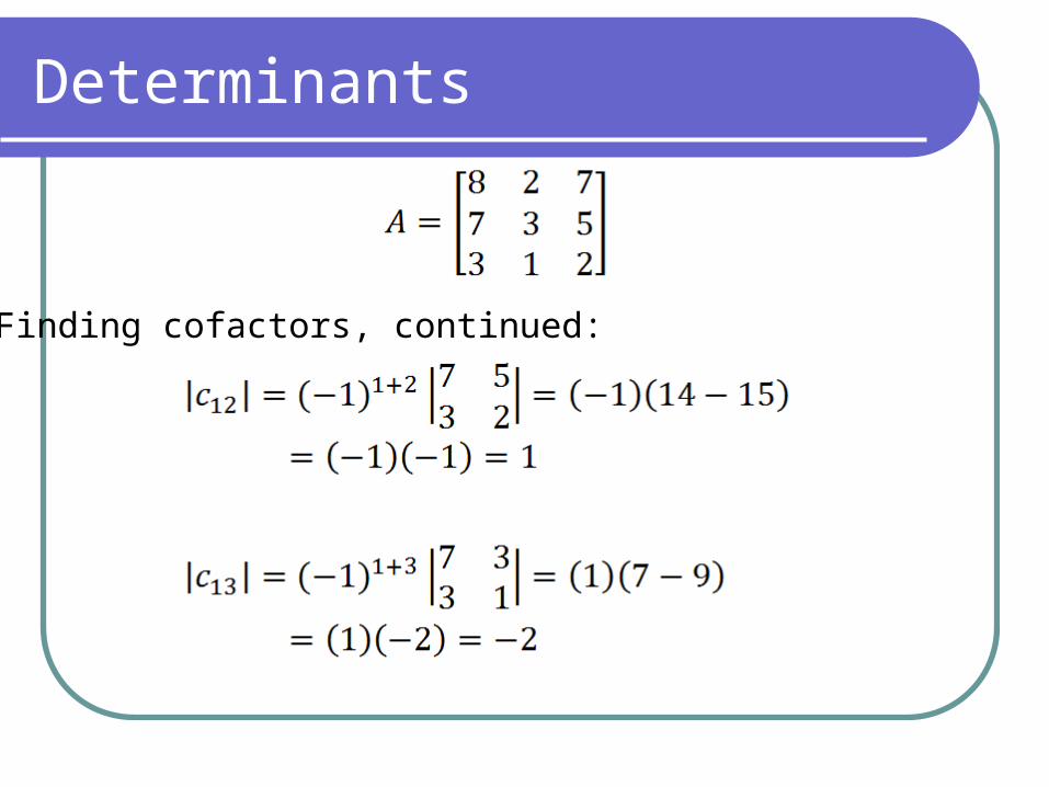
Finding cofactors, continued:

Determinants

Determinants

Or criss-cross method (Chiang)

Determinants

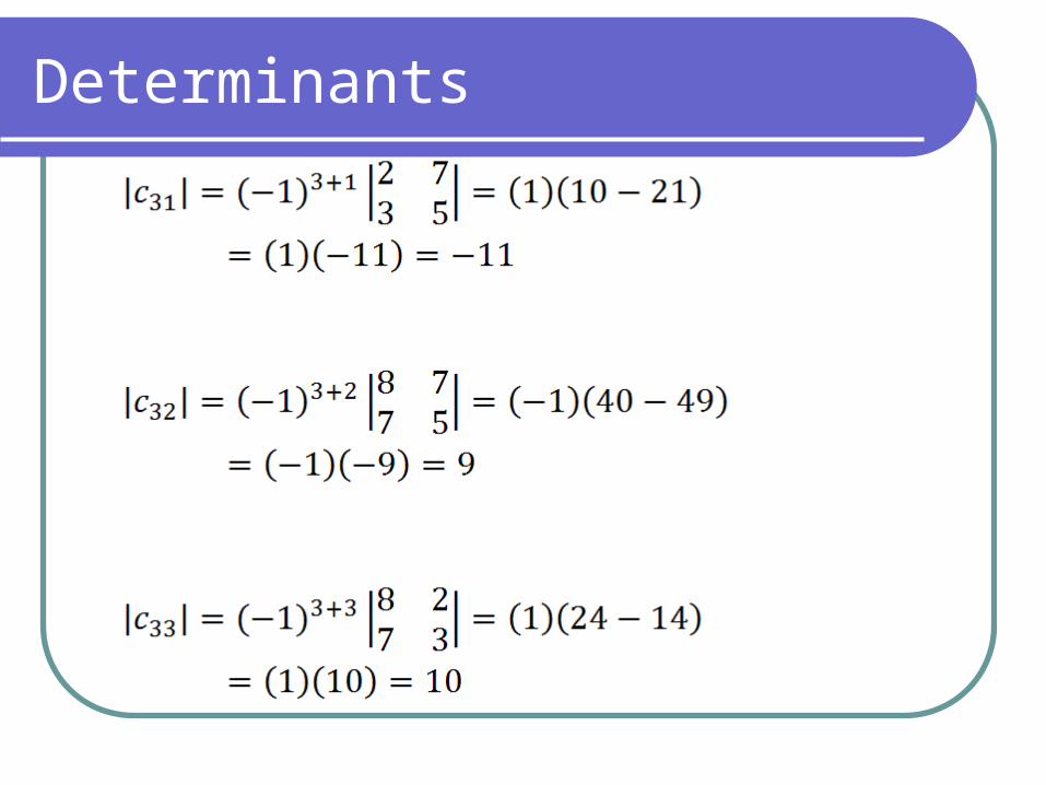
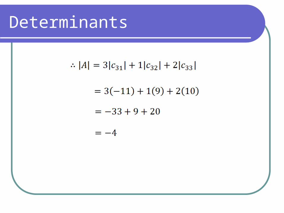
For your own practice, expand by the 3rd row:

Determinants

Determinants

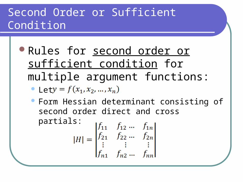
Second Order or Sufficient Condition

Rules for second order or sufficient condition for multiple argument functions: Let Form Hessian determinant consisting of second order direct and cross partials:

Second Order or Sufficient Condition

The first principal minor is defined by deleting all rows and columns except the first row and first column. So, First principal minor

Second Order or Sufficient Condition

The second principal minor is formed by the first and second rows and columns and deleting all other rows and columns So,

Second principal minor

Second Order or Sufficient Condition

The third principal minor: You can use the La Place Transformation procedure or the criss-cross method shown by Chiang to solvefor

Second Order or Sufficient Condition

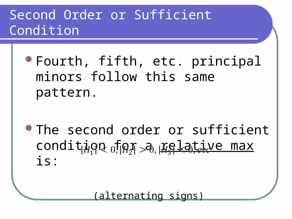
Fourth, fifth, etc. principal minors follow this same pattern.The second order or sufficient condition for a relative max is:

(alternating signs)

Second Order or Sufficient Condition

The second order or sufficient condition for a relative min is:

Second Order or Sufficient Condition

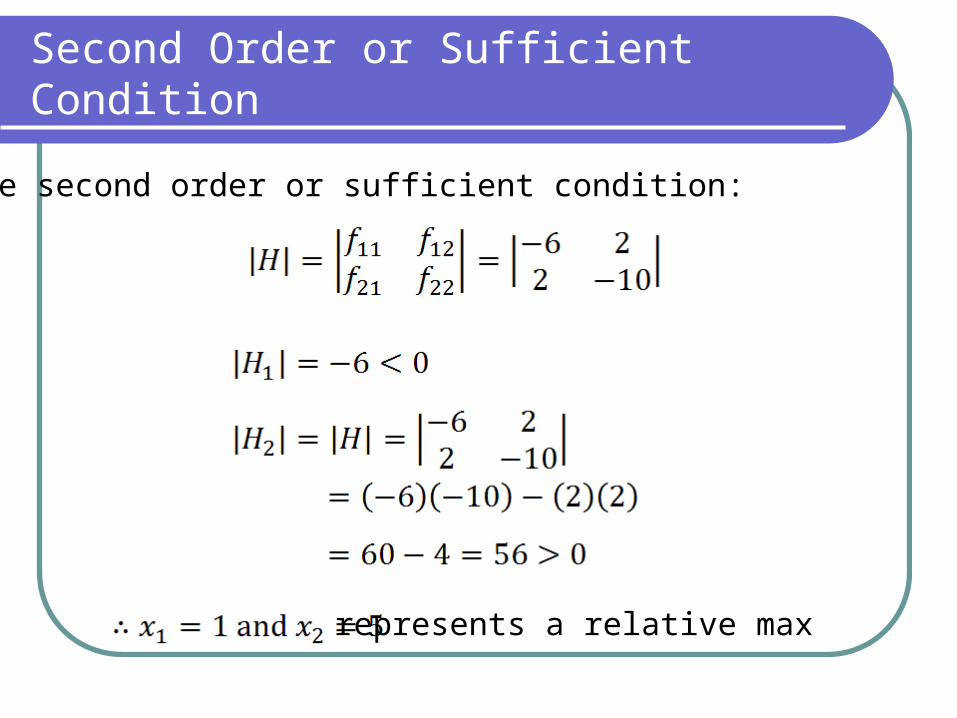
Recall the example:Earlier we found the critical value to be Is this critical value a relative max or min?

Second Order or Sufficient Condition

Use second order or sufficient condition:

represents a relative max