Embed Size (px)
Citation preview
APPLICATIONS OF SHRUB DENDROCHRONOLOGY IN TRACKING DECADAL CHANGES IN
POND MARGIN DYNAMICS
By
Ashley S. Lowcock
A thesis submitted to the Department of Geography In conformity with the requirements for
the degree of Master of Science
Queen’s University Kingston, Ontario, Canada
September 2012
Copyright © Ashley S. Lowcock, 2012

i
Abstract Decadal changes in the surface area of small ponds in the Kluane region, Yukon were quantified from
remote sensing and dendrochronological techniques. Both dead and live shrubs from the genus Salix
were sampled and cross-dated from a total of 28 pond ecotones in two different study areas. The rate of
ecotone shrub colonization was calculated for each pond by determining the minimum age of Salix spp.
in ten zones extending from forest edge to shoreline. Changes in the surface area of 20 ponds in each
study area, for a total of 40 ponds, since 1948 were measured using multi-temporal remote sensing
analysis. Measured changes were then validated using colonization rates derived from the
dendrochronological analysis. Results were compared with meteorological records to elucidate the
connection between climate change and shoreline dynamics.
Ponds experiencing similar rates of ecotone colonization exhibited similar changes in shoreline
position over the last 60 years. Ponds measured with remote sensing showed an overall decline in
surface area since 1948; however, direction and extent of change varied within and between the two
study areas. Colonization rates also varied within and between study areas. This corresponded to
differences in pond ecotone population structure as well as relative extent and direction of changes in
surface area, and supported the changes observed in the low-resolution remote sensing time series
data. Changes in ponds tended to correspond to increases in annual temperatures which, when
combined with a longer growing season and stable precipitation, may have accelerated evaporation
potential causing ponds to decrease. The negative consequences of surface area decline are
exacerbated by the potential increases in evapotranspiration and the much less extensive wetland
system in southwest Yukon relative to other regions in the North. The successful implementation of
remote sensing and dendrochronological techniques has value for remote areas that are sensitive to
climate change, yet lack direct measurement of changing environmental conditions.

ii
Acknowledgments
The completion of this document would not be possible without the continuous support and guidance
of the countless colleagues, friend, family, and peers I’ve been so fortunate to encounter throughout my
graduate experience at Queen’s University. I’d first like to thank my supervisor, Ryan Danby, for
providing the encouragement and opportunity to develop and manage an independent research project
and providing a wealth of knowledge and indispensable guidance in the field of Landscape Ecology. I’m a
better researcher and ecologist because of it. I’d also like to thank my committee members for taking
the time and interest to critically and constructively evaluate the research I’ve completed in Kluane, and
provide a baseline from which to improve future projects. I commend, and am very grateful, to my field
assistants Lucas Brehaut and Katriina O’Kane, along with my honorary field assistant Sinead Murphy, for
remaining in Kluane even after the first day of pond sampling. Measuring 1800 basal stems is no easy
task, so an additional ‘thank you’ goes to Diana Zeng (and Lucas).
This research was funded by an NSERC Discovery Grant and Canada Foundation for Innovation Grant
to Dr. Ryan Danby and an NSTP grant to Ashley Lowcock. Personal funding was received graciously from
the NSERC Alexander Graham Bell Canada Graduate Scholarship and the Ontario Graduate Scholarship
Program. Permission was generously granted by the Champagne and Aishihik First Nations to conduct
this research on their traditional lands, and by Parks Canada to collect samples from the Kluane National
Park and Reserve. Thank you to all the folks at the Kluane Lake Research Station for maintaining an
indispensable Arctic research station in one of the most beautiful regions in Canada, and to Parks
Canada for providing accommodation and a wonderful setting for shrub sampling, without which this
research would not be possible. In particular, I’d like to acknowledge Carmen Wong, the Parks Ecologist
for Kluane National Park and Reserve, for supplying the initial inspiration for the thesis topic and the
continued support and resources necessary in facilitating the completion of this study.

iii
Finally, thank you to my friends and family for pretending to have as much interest as I do in shrub
dendrochronology, remote sensing techniques, and surface area of small ponds in southwestern Yukon.
This mutual understanding from my fellow lab mates, Lyn Garrah, Alix Conway, and Clay McMullen was
particularly valuable. A heartfelt appreciation for the encouragement received by my parents cannot be
overstated, and has continued to motivate me in my many academic pursuits.

iv
Table of Contents
Abstract .......................................................................................................................................................... i
Acknowledgments ......................................................................................................................................... ii
List of Figures ............................................................................................................................................... vi
List of Tables ................................................................................................................................................ vii
List of Abbreviations .................................................................................................................................... viii
CHAPTER 1: INTRODUCTION ............................................................................................................................. 1
CHAPTER 2: COLONIZATION PATTERNS OF SHRUB ESTABLISHMENT WITHIN SMALL POND ECOTONES IN THE
SOUTHWEST YUKON ........................................................................................................................................ 6
2.1 Introduction .................................................................................................................................... 6
2.1.1 Ecotones as landscape features and sentinels for change detection ....................................... 6
2.1.2 Dendrochronology and vegetation dynamics in northern landscapes ...................................... 7
2.1.3 Dendrochronology and changes in transitional ecotone dynamics ........................................... 9
2.1.4 Inferring changes in hydrological regime through transitional boundaries.............................. 11
2.1.5 Objectives ................................................................................................................................ 12
2.2 Methods ....................................................................................................................................... 12
2.2.1 Region of study ....................................................................................................................... 12
2.2.2 Pond selection ......................................................................................................................... 13
2.2.3 Characterization of pond ecotones ......................................................................................... 15
2.2.4 Dendrochronological sampling ................................................................................................ 16
2.2.5 Development of master chronology and cross-dating ............................................................. 18
2.2.6 Seasonal variability and evaluation of dead samples ............................................................. 20
2.2.7 Statistical analysis ................................................................................................................... 20
2.3 Results ........................................................................................................................................ 26
2.3.1 Pond membership based on dissimilarity in pattern of MAoE ................................................ 26
2.3.2 Pond margin population structure ........................................................................................... 27
2.3.3 Pattern of establishment in pond margins ............................................................................... 28
2.3.4 Rates of colonization between groups .................................................................................... 29
2.3.5 Comparison of population structure between pond groups .................................................... 31
2.4 Discussion ................................................................................................................................... 32
2.4.1 Ecotone population structure and association with shoreline behaviour ................................ 32
2.4.2 Colonization rate and association with shoreline behaviour ................................................... 33
2.4.3 The importance of cross-dating in shrub population dynamics ............................................... 36
2.4.4 Ecotone transition and climate change ................................................................................... 37
2.4.5 Implications of transitioning ecotones and diminishing hydrological resources ...................... 41
2.5 Summary ..................................................................................................................................... 42
2.6 References .................................................................................................................................. 43
2.7 Figures and Tables ..................................................................................................................... 52
v
CHAPTER 3: VALIDATION OF MULTI-TEMPORAL REMOTE SENSING OF POND ECOTONES IN SOUTHWEST YUKON
USING DENDROCHRONOLOGY ......................................................................................................................... 61
3.1 Introduction .................................................................................................................................. 61
3.1.1 Inland water surface area decline in the North ....................................................................... 61
3.1.2 Validating change detection of multi-temporal remote sensing with dendrochronology ......... 64
3.1.3 Objectives ................................................................................................................................ 67
3.2 Methods ....................................................................................................................................... 68
3.2.1 Region of study ....................................................................................................................... 68
3.2.2 Pond selection ......................................................................................................................... 69
3.2.3 Image analysis ........................................................................................................................ 70
3.2.4 Assessing shrub minimum age of establishment (MAoE)....................................................... 74
3.2.5 Statistical Analysis................................................................................................................... 78
3.3 Results ........................................................................................................................................ 82
3.3.1 Change in surface area from remote sensing data ................................................................. 82
3.3.2 Shrub establishment and change in pond surface area ......................................................... 83
3.3.3 Evaluating changes in surface area with respect to climate change ...................................... 87
3.4 Discussion ................................................................................................................................... 88
3.4.1 Quantifying water resources in the Arctic ............................................................................... 91
3.4.2 Shoreline behaviour and climate change ................................................................................ 95
3.4.3 The value of wetlands and implications for rapid change ....................................................... 96
3.5 Summary ..................................................................................................................................... 98
3.6 References .................................................................................................................................. 99
3.7 Figures and Tables ................................................................................................................... 107
CHAPTER 4: CONCLUSIONS .......................................................................................................................... 125
APPENDIX A – Prediction of establishment patterns using multivariate regression tree analysis ........... 128
APPENDIX B – Assessment of model assumptions and residuals .......................................................... 130
APPENDIX C – GCP selection and image registration ............................................................................ 136
APPENDIX D – Manual delineation of pond margins ............................................................................... 139
APPENDIX E – Assessment of parametric assumptions for linear mixed modelling ............................. 144
APPENDIX F – Construction and validation of comprehensive climate data for the Kluane Region ....... 146
vi
List of Figures
FIGURE 2-1: KLUANE REGION STUDY SITES FOR SHRUB AGE SAMPLING .................................................................... 52
FIGURE 2-2: SELECTED PONDS FOR FIELD SAMPLING ............................................................................................. 53
FIGURE 2-3: SAMPLING DESIGN FOR PONDS IN THE KLUANE REGION ...................................................................... 54
FIGURE 2-4: STATISTICAL DESIGN FOR MAOE ANALYSIS ........................................................................................ 55
FIGURE 2-5: JOINT PLOT OF CA HELLINGER-TRANSFORMED MAOE DATA. .............................................................. 56
FIGURE 2-6: RELATIONSHIP BETWEEN SL GROUP AND COLONIZATION RATE ............................................................. 57
FIGURE 2-7: RELATIONSHIP BETWEEN DL GROUP AND COLONIZATION RATE ............................................................. 58
FIGURE 2-8: DIFFERENCES IN POPULATION STRUCTURE PER ZONE ........................................................................... 59
FIGURE 3-1: KLUANE REGION STUDY SITES FOR REMOTE SENSING ........................................................................ 107
FIGURE 3-2: AVERAGE MONTHLY ADJUSTED CLIMATE FOR HAINES JUNCTION FROM 1945–2006 ............................. 108
FIGURE 3-3: LOCATION OF SELECTED PONDS FOR REMOTE SENSING AND FIELD SAMPLING ........................................ 109
FIGURE 3-4: TRANSECT DIVISION BY ZONE FROM SHORELINE TO FOREST EDGE ........................................................ 110
FIGURE 3-5: STATISTICAL DESIGN FOR SHORELINE ANALYSIS. ................................................................................ 111
FIGURE 3-6: COMPARISON OF IMAGE QUALITY WITH RESPECT TO SHORELINE ......................................................... 112
FIGURE 3-7: COMPLETE DESSICATION IN DL10 OVER TIME. ................................................................................. 113
FIGURE 3-8: SPATIAL DISTRIBUTION OF SURFACE AREA CHANGE IN SULPHUR LAKE .................................................. 114
FIGURE 3-9: SPATIAL DISTRIBUTION OF SURFACE AREA CHANGE IN DEZADEASH LAKE ............................................... 115
FIGURE 3-10: CHANGE IN STANDARDIZED AREA OVER TIME ................................................................................. 116
FIGURE 3-11: CHANGES IN POND SIZE BY SITE AND YEAR .................................................................................... 117
FIGURE 3-12: CHANGES IN POND STANDARDIZED SURFACE AREA AND SHRUB COLONIZATION .................................... 118
FIGURE 3-13: CHANGE IN TEMPERATURE AND PRECIPITATION SINCE 1945 ............................................................ 119
FIGURE 3-14: DIFFERENCES IN CLIMATE FROM THE MEAN FOR IMAGE YEARS .......................................................... 120
FIGURE A-1: MULTIVARIATE REGRESSION TREE FOR ZONE COLONIZATION DATA IN SULPHUR LAKE ............................. 128
FIGURE A-2: MULTIVARIATE REGRESSION TREE FOR ZONE COLONIZATION DATA IN DEZADEASH LAKE ......................... 129
FIGURE B-1: RESIDUALS FOR PARTIAL NESTING OF THE SL AREA COLONIZATION DATA .............................................. 130
FIGURE B-2: RESIDUALS FOR PARTIAL NESTING OF THE DL AREA COLONIZATION DATA ............................................. 131
FIGURE B-3: ASSESSMENT OF PARAMETRIC ASSUMPTIONS FOR SL RESIDUALS ......................................................... 132
FIGURE B-4: ASSESSMENT OF PARAMETRIC ASSUMPTIONS FOR DL RESIDUALS ........................................................ 133
FIGURE C-1: DIFFERENCE IN SHORELINE TRANSITION WITH PIXEL RESAMPLING ........................................................ 138
FIGURE D-1: BINARY ENCODING OF THE DL34 SHORELINE ................................................................................... 142
FIGURE D-2: AVERAGE AREA OF OPEN POND SURFACE MEASURED PER VERTEX ....................................................... 143
FIGURE E-1: STANDARDIZED RESIDUALS OF SURFACE AREA AT SULPHUR LAKE ......................................................... 144
FIGURE E-2: STANDARDIZED RESIDUALS OF SURFACE AREA AT DEZADEASH LAKE ..................................................... 145
FIGURE F-1: AVERAGE MONTHLY ADJUSTED CLIMATE FOR HAINES JUNCTION FROM 1945–2006 ............................. 148

vii
List of Tables
TABLE 2-1: COMPARISON OF GROUP AND ZONE EFFECT ON ECOTONE SHRUB POPULATION STRUCTURE ......................... 60
TABLE 3-1: IMAGE PROPERTIES FOR AERIAL PHOTOGRAPHS .................................................................................. 121
TABLE 3-2: THE QUANTIFICATION OF POND SURFACE AREA FOR SL PONDS .............................................................. 122
TABLE 3-3: THE QUANTIFICATION OF POND SURFACE AREA FOR DL PONDS ............................................................. 123
TABLE 3-4: LINEAR MIXED EFFECTS MODELS ESTIMATING CHANGE IN SHORELINE OVER TIME ...................................... 124
TABLE B-1: EIGENVECTORS AND PROPORTION OF INERTIA EXPLAINED FOR CORRESPONDENCE ANALYSIS....................... 134
TABLE B-2: LINEAR MIXED EFFECTS MODEL SELECTION......................................................................................... 135

viii
List of Abbreviations POND TYPOLOGIES: HGT HEIGHT DDS DENSITY OF DEAD SHRUBS DDS DENSITY OF DEAD STEMS DLR DENSITY OF LIVE STEMS DLS DENSITY OF LIVE SHRUBS PDR PROPORTION OF DEAD STEMS STUDY AREAS: DL DEZADEASH LAKE SL SULPHUR LAKE STATISTICAL ANALYSIS AND DESIGN: CA CORRESPONDENCE ANALYSIS UPGMA UNWEIGHTED PAIR-GROUP METHOD USING ARITHMETIC AVERAGES MAOE MINIMUM AGE OF ESTABLISHMENT MRT MULTIVARIATE REGRESSION TREE
1
CHAPTER 1: INTRODUCTION
Evidence for accelerated climate warming has been well documented in northern regions, where
ecosystems are characterized by a high degree of sensitivity to external environmental forcing as well as
isolation from the direct anthropogenic disturbance typically experienced at lower latitudes. The Arctic,
defined as regions north of 60° latitude, has experienced a reduction in sea-ice cover, a northward
retreat of permafrost boundaries, altered hydrological dynamics, changes in biogeochemical processes,
and shifts in vegetation community structure and extent (Rouse et al., 1997; Serreze et al., 2000; ACIA,
2005; Hinzman et al., 2005; Myers-Smith et al., 2011a). Under a changing climate regime, significant
changes in ecosystem functioning and surface water balance are expected to continue (e.g. Rouse et al.,
1997; Hinzman et al., 2005).
Research into the landscape ecology of northern regions is largely focused on changes in vegetation
dynamics and hydrological processes; typically attributed to amplified climate warming. An emergent
topic in the field of landscape ecology is the response of ecotones – the zone of community transition
between adjacent ecosystems – to climate warming (e.g. Kent et al., 1997; Peters et al., 2006; Bekker
and Malanson, 2008; Hofgaard et al., 2010). Due to the nature of ecotone formation, which is the result
of complex interactions between adjacent ecosystems, ecotones are spatially confined and detectible at
multiple scales, constituent species are heterogeneously distributed, and communities are sensitive to
changes occurring within their contributing ecotypes. Changes in atmospheric conditions are, therefore,
expected to promote more detectable responses within transition zones than reflected by the
landscape. Due to this combined sensitivity and detectability, Bekker and Malanson (2008) regard
ecotones as ‘sentinels’ for climate change, warranting further investigation into the behavior of these
systems.

2
Germane to the understanding of ecotone dynamics in Arctic and sub-Arctic regions are two
emergent themes in landscape ecology. The first is the expansion of woody vegetation into previously
herbaceous latitudinal and altitudinal vegetation zones – a phenomenon known as shrubification. The
second theme is related to the ubiquitous decline or disappearance of small inland lakes and ponds. A
rapid progression of both trends has been observed over the last few decades and each are well
documented in the literature (e.g. Stow et al., 2004; Schindler and Smol, 2006; White et al., 2007;
Myers-Smith et al., 2011a). A common technique linking these two themes is the use of a multi-
temporal remote sensing series in order to detect changes occurring from historical images to more
recent photographs of the same area, or to modern satellite imagery.
Pond shorelines mark the transition from the open water to terrestrial upland vegetation making
them particularly easy to identify. Shoreline behavior is also quite sensitive to small changes in regional
climate (e.g. Smol and Douglas, 2007; Adrian et al., 2009; Williamson; Adrian et al., 2009). As a result,
changes in shoreline position, typically measured through changes in pond surface area, have been
studied largely via remote sensing (e.g. Yoshikawa and Hinzman, 2003; Smith et al., 2005; Riordan et al.,
2006). However, due to the high number of optical satellite imaging products available, the variability
inherent in aerial photography, and the lack of consistency in methodology used to quantify lake surface
area, results from each study are difficult to compare.
In addition to technical and methodological issues with this technique, practical issues include the
omission of: (1) seasonal processes not captured by the temporally static images; (2) spatial variability
across the landscape, where images are only available for a limited number of sites; or (3) dynamic
processes occurring in the interim of years for which remotely sensed images are available. This is a
particular problem in northern regions, where the heterogeneous nature of the landscape, along with
the inadequate spatial coverage and temporally deficient historical data, limits the ability to make
definitive statements about long term trends and spatial distribution in vegetation and hydrological

3
resource dynamics. Data in the North is lacking in both quality and quantity, where resolution of
timescales and spatial coverage is small; with a set of two or three generally poor quality historical
images available for any given study area, and then typically in areas along features of economic or
anthropocentric importance, such as major roads or settlements.
In order to validate the trends in pond area changes, reported from image analysis, the processes
occurring between images also need to be quantified. The conditions within the pond ecotone – the
transition between the aquatic and mature upland terrestrial communities – reflect both the
hydrological processes and vegetation dynamics occurring at the interface of upland terrestrial and
pond ecosystems. As open water recedes, the surrounding terrestrial ecotone advances as the ‘barrier
effect’ of open water is removed and new areas available for colonization are exposed. Shrub expansion
in this zone, and thus changes in waterline over time, can be quantified through methods used in
dendrochronology – a technique for quantifying natural processes through the character of tree ring
structure or the dating of tree ring formation (Speer, 2010). A lack of direct observation in northern
landscapes creates a need for researchers to make use of the natural record of change provided by the
landscape.
Dendrohydrology is a relatively new sub-field of dendrochronology and is based on the predictable
growth processes of woody plant species, the timing of establishment under changing hydrological
processes (ecesis), and the effects of shoreline dynamics on tree growth. Although the application of the
dendrochronological process and cross dating of shrubs is relatively recent, and less tested than that for
trees, there has been success in this field (see Myers-Smith et al., 2011a). Research into shrub expansion
has provided evidence for the ability of tall shrubs to quickly take advantage of environmental
conditions suitable for growth, especially under a warming climate (Elmendorf et al., 2012). Vegetation
dynamics are less sensitive to seasonal changes, in that responses to short term climate events will not
be as dramatic as water level dynamics in small ponds. Therefore, estimates of shoreline recession

4
based on measurable changes in vegetation dynamics are more seasonally reliable than low resolution
images of waterline.
The objectives for this Masters research project were to: (1) Characterize the patterns of shrub
establishment in the ecotone of small ponds in the Kluane Region of the southwest Yukon using
dendrochronological techniques; (2) Investigate the association of shrub establishment with
hydrological regimes in the pond ecotone; (3) Quantify changing pond shorelines in the Kluane Region
using remote sensing techniques; (4) Assess the validity of remotely sensed time series by
supplementing the low resolution timeline with a continuous natural chronological record found
through the principles of dendrochronology; and (5) Determine the role of climate in influencing pond
ecotone dynamics.
Successful completion of these objectives required that, first, appropriate closed basin ponds were
selected using satellite imagery. Second, the connection between hydrological regime and vegetation
dynamics was determined through the relationship between pattern of shrub establishment, ecotone
population structure, and change in surface area. Third, for each field sampled pond, surface area over
the last 60 years was measured and quantified in aerial photographs and QuickBird data acquired during
the summer, at different time periods. Chronologies of pond shoreline recession were generated by
determining ecotone colonization rates by Salix spp. and were used to validate trends observed through
remote sensing techniques. Finally, a possible connection with climate change, as a possible driving
mechanism for change in surface area, was discerned through climate records for the timeline and
region of study. Records were qualitatively compared with the trends in surface area change and
chronologies of shoreline position in the Kluane Region, developed from the two techniques.
The diverse landscape and climate regime of the Kluane region of the southwest Yukon was well
suited to the objectives of this study: an Arctic boreal ecosystem underlain by scattered discontinuous
permafrost, characterized by variable terrain and spatially distinct climate regimes. These environmental

5
conditions are less substantially quantified in terms of pond surface area dynamics, and exhibit
characteristics similar to inland freshwater bodies found in previous studies. The Kluane Region has also
experienced some of the most significant climate warming in the Arctic over the last 40 years (ACIA,
2005). The majority of ponds in the Yukon are shallow open water ponds (Janowicz, 2004), represented
by those in the current study, which are most susceptible to small changes in environmental conditions
(Carroll et al., 2011). Wetlands in the region are essential for hydrologic storage, filtering and wildlife
habitat, and the implications of surface area change are exacerbated by the much less extensive wetland
system relative to other areas in the North (Janowicz, 2004).

6
CHAPTER 2: COLONIZATION PATTERNS OF SHRUB ESTABLISHMENT WITHIN SMALL POND ECOTONES IN
THE SOUTHWEST YUKON
2.1 Introduction
2.1.1 Ecotones as landscape features and sentinels for change detection
Landscapes are broken up by ecotones, the transitions between adjacent ecosystems. Although
ecotones are dynamic functional zones with self-organizing community types, changes in structure,
composition and processes reflect the changes occurring within each adjoining ecosystem (Strayer et al.,
2003; Yarrow and Marin, 2007). Given the narrow and heterogeneous spatial distribution of transition
zones, relative to the contributing patch types, ecotones are presumed to be particularly sensitive to
changes in climatic conditions making them potential indicators of environmental change (e.g. Kent et
al., 1997; Peters et al., 2006; Bekker and Malanson, 2008; Hofgaard et al., 2010). Due to the important
role of ecotones in the functioning of landscape processes, research into the understanding of these
features is becoming a focal point in landscape ecology (e.g. Strayer et al., 2003; Yarrow and Marin,
2007; Bekker and Malanson, 2008), including their potential value in evaluating changes in climatic
regimes (Epstein et al., 2004; Smith et al., 2009; Kent et al., 1997; Peters et al., 2006; Bekker and
Malanson, 2008; Hofgaard et al., 2010). This is particularly true for northern landscapes, where rapid,
dynamic changes are likely to occur in response to a warming climate, altering both the ecology and
function of the region (Epstein et al., 2004).
The distinct boundary between adjacent aquatic and upland terrestrial ecosystems, typically referred
to as the shoreline (Strayer and Findlay, 2010), imposes easily identifiable limits and constraints on pond
ecotone formation and function. The pond ecotone is defined here as the transition zone between open
water and the mature boreal ecosystem. This contrast of contributing ecosystems makes shoreline
boundaries relatively easy to define and measure both in the field and through remote sensing (Sannel
and Brown, 2010). Northern inland water bodies are also particularly sensitive to small changes in
7
regional climate (e.g. Smol and Douglas, 2007; Adrian et al., 2009; Williamson), making these transition
zones potentially valuable proxies in measuring ecosystem changes in response to external influence,
such as climate forcing (Adrian et al., 2009).
Despite the distinctive nature of shoreline boundaries, the formation, composition, and processes
within pond ecotones are complex. Within the boreal forest ecosystem, shifts in edge-of-forest
communities occur alongside a dynamic pond shoreline. As open water recedes, the surrounding
terrestrial ecotone advances as the ‘barrier effect’ of open water is removed and new areas available for
colonization are exposed; as water levels rise these individuals die off leaving a break in the record. The
influence of a warming climate on the recent success of tall shrub establishment (Myers-Smith et al.,
2011a) has made dendrochronology a prospective technique for developing a continuous record of open
water dynamics in the Arctic. The expansion of shrub species has been well documented in the North,
particularly at grassland and tundra boundaries, where dendroecological studies have shown the rate
and timing of forest expansion in arctic and alpine environments.
The current study characterized changes in pond ecotone dynamics responding to recent climate
warming in the Kluane Region of the southwestern Yukon, a region that has seen some of the highest
temperature increases in the North over the last half century. The quantification of vegetation
establishment within pond ecotones near Haines Junction YT (60°45′10″ N, 137°30’24” W), was applied
as a metric for shoreline behaviour of small, inland ponds. The utility of ecotones in detecting changes
over the landscape is discussed in the following sections.
2.1.2 Dendrochronology and vegetation dynamics in northern landscapes
Evidence for accelerated climate warming has been well documented in northern regions; where
ecosystems are characterized by both a high degree of sensitivity to external influence and isolation
from the direct anthropogenic disturbance typically experienced in the lower latitudes. Under a
changing climate regime, the Arctic has experienced a reduction in sea-ice cover, a northward retreat of
8
permafrost boundaries, altered hydrological dynamics, changes in biogeochemical processes, and shifts
in vegetation community structure and extent (Rouse et al., 1997; Serreze et al., 2000; ACIA, 2005;
Hinzman et al., 2005; Myers-Smith et al., 2011a). Each response contributes to a broader change in the
landscape ecology of the region.
Recently, Arctic and sub-Arctic regions have seen a surge in common colonial shrub expansion into
previously herbaceous vegetation zones, both at high latitudes and in alpine environments, at the
physiological limit of woody vegetation growth (Sturm et al., 2001; Tape et al., 2006). As tall shrub
species outcompete most other woody vegetation types (Elmendorf et al., 2012), changes are visible
using high resolution images available through remote sensing (Stow et al., 2004; Tape et al., 2006;
Danby and Hik, 2007a; Myers-Smith et al., 2011a; Naito and Cairns, 2011). In addition, the shrubification
of the Arctic (Myers-Smith et al., 2011a), is likely the catalyst for the growing exploitation of shrub
species in studies employing dendrochronological techniques – the use of tree-ring analysis in the
reconstruction of natural processes and anthropogenic phenomena (Speer, 2010). Although
dendrochronological studies using non-tree species remain relatively uncommon in the literature, being
almost exclusive to the Arctic region, this application of dendrochronological research can offer insight
into the behaviour and chronosequencing of short term, highly variable, environmental processes.
A broad scale exploration of vegetation change in the Alaskan Arctic found that over half of all areas
surveyed experienced an increase in growth and abundance of shrubs with none of the areas
experiencing a reduction after 50 years (Sturm et al., 2001). The lack of human and natural disturbance
suggested that these changes were induced by the recent climate warming experienced in the region.
Several studies have since confirmed these findings using repeat photography, plot level studies, and
satellite remote sensing (Tape et al., 2006; Danby and Hik, 2007ab; Myers-Smith et al., 2011b; Naito and
Cairns, 2011) as well as dendrochronology (Hallinger et al., 2010; Myers-Smith et al., 2011b). While the
majority of recent shrub research has focused on shrub encroachment into arctic and alpine tundra

9
ecosystems, investigations into shrub dynamics have greatly improved our understanding of a variety of
ecosystem processes. Dendrochronology has been used to elucidate the rate of vegetation expansion
(Myers-Smith et al., 2011b), rates of isostatic rebound (Bégin and Filion, 1995), shoreline reconstruction
(Bégin and Payette, 1988; Bégin 1996), and flood plain hydrology (Bégin and Payette, 1991); validation
that this valuable technique has the potential to aid in the quantification of changes occurring in
multiple landscape processes.
2.1.3 Dendrochronology and changes in ecotone dynamics
Complex interactions between geomorphology, environmental gradients, and species dispersal,
establishment and interactions, influence ecotone assemblage and connectivity over time and across
spatial scales (Peters et al., 2006). This complexity impedes the ability to determine which components
of these systems can be attributed to changes in environmental conditions, and how the changes
observed reflect changes in the surrounding landscape. Plant zonation along lakeshores has been
characterized by several authors (see Strayer and Findlay, 2010 for a review), and is particularly relevant
to the understanding of ecotone dynamics in relation to environmental gradients. The pattern is likely to
reflect outcomes of interspecies competition for resources in the gradient of environments from
shoreline to the forest ecosystem, with certain woody vegetative species able to expand into particularly
inaccessible areas of shoreline during periods of low water levels.
Pond ecotones represent a group of ecosystem boundaries known as directional transition zones,
which essentially develop as a result of the displacement of species characterizing one ecosystem type
by that of another (Cadenasso et al., 2003). These directional shifts allow for in-depth characterizations
of community succession in response to a dynamic ‘disturbance margin’ in the absence of confounding
variables from a competing ecotype. There exists invaluable potential for the characterization and
chronosequencing of ecosystem processes, particularly through dendrochronology.

10
There have been consistent findings for hydrological variables, as the main factor in the
development of terrestrial vegetation patterns along shorelines (Keddy and Reznicek, 1986; Yabe and
Onimaru, 1997; Klein et al., 2005; Breeuwer et al., 2009), despite potential variability in chemical or
physical properties of shoreline (Jabłońska et al., 2011). The receding shoreline of a drying pond
represents the removal of a physical constraint to species dispersal and establishment, with the
subsequent succession of upland terrestrial vegetation into the catchment area representing shifting
transition zones. The directional nature of the transition zone, resulting from this lack of contributing
source populations from the pond ecotype, should depend on the recession or expansion of pond
shoreline.
The predictable response of vegetation to water level fluctuations can then be used to assess the
timing of past shoreline position through the recessional movement of the pond ecosystem and the
forward expansion of the upland terrestrial ecosystem. This principle was employed by Bégin (1993) to
assess the utility of tree and shrub growth in characterizing transgressing shorelines and by Filion and
Bégin (1995) to calculate rate of isostatic rebound from regressing waterline of Lake Bienville in
subarctic Quebec. More recently, Roach et al. (2011) determined the ages of trees and shrubs within the
pond ecotone of both decreasing and nondecreasing boreal lakes to evaluate the drying of lake beds as
a possible mechanism for decreasing ponds in southern Alaska. The authors found that trees and shrubs
closest to the pond margin were significantly younger in lakes experiencing a decline in surface area
than in those showing an increase.
Shrub dendrochronology is a fairly new development and is subject to a number of assumptions
which can lead to greater inaccuracies (Bégin and Payette, 1991; Speer et al., 2010; Myers-Smith et al.,
2011a). Shrubs generally exhibit irregular growth forms which determine the eccentricity,
distinctiveness and presence of growth rings, and therefore their utility in dendronchronology
(Kolishchuk, 1990; Speer, 2010; Schweingruber et al., 2011). Although the application of the

11
dendrochronological process and cross-dating of shrubs is relatively recent and less tested than that for
trees, much success has been achieved at Arctic treeline and shorelines of large-scale sub-Arctic lake
systems; where several studies have validated the application of shrub establishment and
metapopulation dynamics in estimating rates of physical and ecological processes at the ecotone
boundary (e.g. Bégin and Payette, 1991; Bégin and Filion, 1995; Forbes et al., 2010; Hallinger et al.,
2010; Myers-Smith et al., 2011b).
2.1.4 Inferring changes in hydrological regime through transitional boundaries
The quality of hydrological monitoring in the North has been criticized by several authors (e.g. Serreze
et al., 2000; Bring and Destouni, 2011; Carroll et al., 2011). Bring and Destouni (2011) note that those
regions projected to, or currently experiencing, the greatest changes in precipitation possess the lowest
density of meteorological stations, including the southwest Yukon. It is not surprising that, save for
large, recreationally important lakes and rivers, direct measurements of inland freshwater systems are
generally absent in remote regions such as Kluane, YT. For this reason, it is not possible to develop
accurate ring-width chronologies of potentially episodic high water levels, since we cannot relate these
events to concurrent ring-width reaction in shrub species. In addition, ring-widths in shrub species may
not cross-correlate well, if at all, making comparisons with reference populations beyond the exposed
catchment area potentially misleading.
Alternatively, the rapid response of shrubs to changes in local environmental gradients provides
information on rate of shoreline recession and expansion on decadal scales (Bégin, 1990; Von Mörs and
Bégin, 1993). Age frequency dynamics reflect shoreline exposure and local conditions, while growth
forms and scarring provide a near annual chronology of extreme events and complex shoreline
disturbance regimes (Von Mörs and Bégin, 1993; Bégin and Filion, 1995). Shrub populations will migrate
up shorelines, with abrupt shrub ecotone zonation and very little seedling survival under conditions of
lake level rise or stable shorelines with predictable disturbance regimes. In contrast, populations will

12
show a mosaicked, yet predictable, response to unstable shoreline conditions and rapidly expand
inwards towards retreating shorelines as suitable sites become available.
While age classification, for metapopulation studies such as these, has successfully substituted cross-
dating techniques (Von Mörs and Bégin, 1993), it requires prior knowledge of the final ring age, meaning
that age classification can only be applied to living samples. Earlier establishment is omitted, potentially
biasing interpretation of results. In the absence of more direct measurement, the use of
dendrochronology in determining an annual resolution of shrub establishment, in newly available sites
within the ecotone, provides an additional approach for quantifying recent shoreline behaviour in small
sub-Arctic ponds (Von Mörs and Bégin, 1993).
2.1.5 Objectives
The objective for this study was to utilize shrub dendrochronology as a metric for quantifying changes
in pond ecotones and characterizing shoreline behavior. This objective was accomplished by: 1)
Assessing differences in recent shoreline change among small ponds in southwest Yukon by comparing
patterns of shrub age across their ecotones; 2) Evaluating establishment patterns and colonization rates
of pond margins in association with shrub population structure; and 3) Assessing the value of cross-
dating in the development of shrub chronologies through the inclusion of non-living shrub
establishment.
2.2 Methods
2.2.1 Region of study
The Kluane National Park and Reserve and the Kluane Wildlife Sanctuary are located in the southwest
corner of the Yukon. Generalizations about climate in the Kluane Region are difficult due to the diverse
topography which produces highly variable wind patterns, solar radiation availability, and moisture
regimes within short distances (Gray, 1987). However, there are distinct north-south transitions, as well
as maritime-continental climatic divides. At the northern end, in the Donjek Valley, the moisture regime
13
is dry, temperatures are lower, and the soil is underlain by discontinuous permafrost. In the south,
climate is warmer and moister with greater soil development, and denser forests and wetland
vegetation.
Wetlands are generally associated with major lakes which include Kluane, Kloo, Dezadeash, Kathleen,
Mush and Bates Lakes. These lakes are supplied and drained by extensive fluvial systems. This region
has been inundated several times over the past few hundred years as a result of glacial blockages across
the Alsek River (Yukon Ecoregions Working Group, 2004). Relative to other areas in the Arctic, or sub-
Arctic, the Yukon does not possess extensive systems of wetlands, which cover less than 5% of the
Territory, and the majority are composed of shallow open water ponds. Two areas of interest were
selected for this study. These were characterized by a large number of small ponds, generally accessible
from the Alaska Highway (Fig 2-1).
Both areas occupy the Ruby Ranges ecoregion; one of the driest regions in the Territory due to its
geographic location in the rain shadow of the St Elias Mountains (Gray, 1987). The majority of ponds in
the study areas are found within the Aishihik Drainage Basin, which is drained by the Alsek River to the
Gulf of Alaska and comprises 4% (19,000 km2) of the Territory (Janowics, 2004). Ponds of interest are
scattered along the Shakwak Trench in the region southeast of Kluane Lake; falling within the sporadic
discontinuous permafrost zone. Permafrost near Haines Junction has been recorded at 7.3m but most
of the ground is only seasonally frozen (Yukon Ecoregions Working Group, 2004).
2.2.2 Pond selection
The study region was subdivided into two areas to account for a regional north-south climate
gradient, referred to as the Sulphur Lake (SL) and Dezadeash Lake (DL) areas (Fig 2-2). An inventory of all
potential ponds in each region was generated using NTS map sheets and Google Earth v.6.1.0.5001
imagery (Google Inc., 2011). Suitable ponds were selected based on a set of criteria that would control
for the influence of geomorphic and topographical factors while maximizing the number of ponds that

14
could be sampled in the field. Potential inclusion of each pond was evaluated based on a set of criteria
intended to evaluate comparable patterns of shrub establishment that accurately represented shoreline
dynamics across both the SL and DL study areas.
First, a symmetrical shape was considered; with desirable ponds possessing a length-to-width ratio
close to 1:1. Ponds that deviate from a circular shape are more likely to be bathymetrically
asymmetrical, resulting in dissimilar environmental gradients depending of the aspect sampled, which in
turn results in a variable community structure and ecesis. Second, any edge effects from secondary
roads and the Alaska Highway, or from forest clearing for the pipeline right-of-way, may also impact the
establishment, survival, and age structure of surrounding vegetation (see Harper et al., 2005). To
mitigate edge effects of this nature, ponds which were isolated from anthropogenic disturbance were
desirable, however, ponds still needed to be accessible on foot from the Alaska Highway. Finally, the
assessment of potential effects of climate on shoreline was facilitated by restricting analysis to closed-
basin ponds, defined as ponds having no visible surface connection to nearby fluvial systems. This
characteristic facilitates the isolation of climate forcing with respect to the precipitation-evaporation
ratio, evapotranspiration, and permafrost dynamics (Anderson et al., 2007; Abnizova and Young, 2009;
Roach et al., 2011). It also reduces the confounding effects of seasonal variability associated with natural
fluctuation in fluvial systems including the Alsek, Jarvis, and Dezadeash Rivers.
Once all suitable ponds were identified, fourteen ponds from each study area were randomly
selected for analysis and sampling in the field. A minimum impact philosophy was used to guide all field
related activities and Parks Canada protocol for scientific field work was followed at all sites.
Unnecessary trampling of vegetation and wildlife disturbance was minimized. Because anurans are
particularly susceptible to Chytridiomycota, boots were rinsed in a diluted bleach solution prior to pond
visitation to prevent the introduction of the fungus into the National Park. In addition, noise was kept to

15
a minimum when sampling at ponds where the presence of waterfowl was evident, and the nest sites of
wetland species, such as trumpeter swans, and wood frog egg masses were avoided.
2.2.3 Characterization of pond ecotones
Depending on the scale of observation, shoreline is typically defined as the point where water is
separated from land, which is almost impossible to define (Strayer and Findlay, 2010). Shoreline has also
been described as the point where the water table falls below the surface (Roach et al., 2011). However,
initial surveys revealed some ponds where shrubs persisted beyond this point, in some cases as far into
the pond area as emergent vegetation. Therefore, shoreline was defined as the point where open water
transitioned to emergent vegetation, which proved to be well defined in the majority of field sampled
ponds.
The definition of the pond margin ecotone is even more ambiguous than shoreline, often dependent
on the objective of the study undertaken (Strayer and Findlay, 2010). Here I defined the pond ecotone
as the area of vegetation spanning the shoreline to forest edge, as this community has most likely been
influenced by the hydrological regime of the pond. The forest edge was defined as the zone in which the
vegetation community transitioned to spruce dominated forest. In cases where this transition was
unclear, or at uninformative distances, a significant change in slope, where an obvious levelling of relief
occurred, was taken as the perceptible limit of former pond bathymetry. In the majority of cases these
criteria corresponded quite well.
At each pond, the ecotone was divided into three areas of similar community structure with respect
to shrub population characteristics (density, size and vitality). A transect was established randomly
within each area, perpendicular to shoreline and spanning the entire ecotone (Fig 2-3). Similar
community structures were selected for transect placement in order to minimize potential zonation of
establishment resulting from variability in environmental gradients parallel to the shoreline (Bendix,
1994), rather than the advance of colonization front as a result of a retreating shoreline (Bégin, 1989).

16
Because the degree of slope from forest edge to shoreline plays a role in hydrological regime, a major
factor in determining establishment of surrounding terrestrial vegetation (Strayer and Findlay, 2010),
the slope of all pond margins was kept consistent between transects and ponds.
Individual shrubs found within one meter of each transect were measured for: distance from open
waterline and from transect, plant status (alive or dead), live and dead basal stem count, height of the
tallest live stem, and coverage area (measure of crown length and width). These metrics were used to
characterize both zonal and pond ecotone population structure, including: live and dead shrub density
(m2), live and dead stem density (m2), proportion of live and dead stems, average shrub size, and tree
density (m2). Individual shrubs were defined by the ability of the recorder to establish below-ground
connections. Stems emerging from a common root collar were considered to be members of the same
individual.
In some cases it was not possible to begin each transect at the pond shoreline. This included ponds
SL-144 and SL-152, which were too deep to access, and the shoreline of DL-08 which was more than 50
meters from the furthest shrub establishment in relation to the forest edge. In these cases, transects
were established from the forest edge toward open water for a maximum distance of 30 meters.
Although this could potentially influence the pattern of minimum age of establishment across the zones
in each of these ponds, the high water levels suggest that woody vegetation would have been unable to
establish successfully in these areas.
2.2.4 Dendrochronological sampling
For the collection of dendrochronological samples, transects were divided longitudinally into ten
equally sized transition zones that were 2 meters wide on either side of the transect. Zone A
represented the transition zone closest to pond edge, and J represented the zone closest to forest (Fig 2-
3). In this way, the size of each plot was relative to the length of the transect, allowing for inter- and
intra-pond comparison of transects.

17
The dendrochronological response of shrubs may differ significantly by taxa, therefore only the
dominant genus was chosen for the current study. Salix spp. were clearly the dominant shrub type at all
but the two higher elevation ponds (> 1000 a.s.l.), and was therefore chosen for sampling across the
entire region. Salix spp., in particular, are prominent tall shrubs on the landscape that are well suited to
moist soil environments and are likely to minimize ecesis, establishing much more rapidly than either
spruce or other shrub species. Sampling was restricted to tall Salix spp., to minimize issues related to
compact and uninformative ring formation (Schweingruber et al., 2011).
Typically, shrubs should be sampled at the basal cormus, the complex woody structure formed by
coalescence of stems and roots at the collar, as this segment corresponds to the original germination
level (White, 1979). Shrubs are not only highly clonal, which complicates separation of individuals and
assessment of the age of establishment, but they are also rhizome-based plants which do not typically
produce a ring of equal width, or at all, throughout the entire length of each stem (Kolishchuk, 1990;
Speer, 2010; Schweingruber et al., 2011). Many authors avoid cross-dating among shrub species
individuals, reporting ring widths which rarely correlate within shoots of the same plant, let alone
between individuals (Von Mörs and Bégin, 1993; Kolishchuk, 1990; Speers, 2010). However, success in
shrub dendrochronology has recently been shown in Arctic shrubs (see Myers-Smith et al., 2011a). In
addition, a great deal of information may be lost without the annual resolution provided through
dendrochronological analysis, which is founded on cross-dating of ring-widths.
The resources required to sample each individual at the cormus, for a study of this size, are not
practically available, nor would the destructive nature of this form of dendrochronological sampling be
acceptable within national park boundaries. A more practical approach was taken to estimate the
earliest date at which a given site in the pond ecotone was made available for establishment; that is, the
timing of shoreline retreat. Assuming that the largest central stem is generally the dominant and
18
therefore earliest growing stem, the three largest live basal stems in each zone were sampled and their
ages determined.
In order to determine the absolute date of establishment, and account for irregular or missing rings,
the entire root collar must be extracted and each stem serial sectioned in accordance with Kolishchuk
(1990) to properly age each stem. Even then, the determined age indicates the absolute age of the
clone, and not necessarily the parent individual. These methods are time consuming, and would result
in a reduction of sample size. Bégin et al. (1989) found that the age structures of willow shoots did
follow a similar pattern to collar ages; therefore, a trade-off was made between the number of ponds
assessed and shrub sample size, where only one section for each stem was collected for analysis.
Sections were acquired as close to the true root collar as possible. Personal observation confirmed that
collar ring widths were much more eccentric and prone to misidentification than those found
throughout the stem. Because willows typically establish by seed on moist substrate (Bégin and Filion,
1995), each group was likely a genetic individual and a reflection of first establishment. Since the
objective is to determine the relative ages of establishment in order to develop a pattern of shoreline
colonization, this trade-off was considered acceptable.
2.2.5 Development of master chronology and cross-dating
Sample sections were progressively sanded down to a grit level of 600, and then ring-width time-
series were measured to the nearest 0.001 mm using a Velmex “TA” system (Velmex Inc., Bloomfield,
NY) in conjunction with the MeasureJ2X software v.4.1.2 (VoorTech Consulting, Holderness, NH). The
diameter of each section was measured and age was determined for each sample. The average size of
the oldest stem in each zone (calculated as cross-section area in mm2) was significantly larger than the
average of the youngest stem (152.6 ±31.9mm2, t = 4.788, p< 0.0001), validating our assumption that
dominant stems are typically older. In addition, the odds of the smallest stem being oldest decreased by
19
a factor of 2.35 when compared to any other size, providing evidence that a sample of the three largest
stems likely captures the minimum age of establishment for that zone.
A chronological profile was generated for each transect from the open water edge to the upland
forest edge. Larger sections with clearly defined rings were used to create master ring-width
chronologies for each pond. Master chronologies were validated using the dendrochronology software
COFECHA version 6.06 (Holmes, 1983) to the point where recommended shifts in flagged sections did
not significantly increase the correlation among sample chronologies. The limitation in sample depth
(i.e. the average age of the shrub population) made this necessary, as COFECHA cannot adequately
evaluate samples younger than about 60 years. Because the average sample depth was younger than 60
years, validating time series with every sample would potentially result in spuriously high or low
correlations (Grissino-Mayer, 2001).
The remaining samples were cross-dated visually and correlated in accordance with COFECHA
software, where a Pearson’s correlation coefficient of 0.42 was the minimum value necessary to be
considered well correlated. Adding missing rings and removing potentially false rings was avoided unless
the change visually improved or significantly changed sample correlation with the master chronology.
The number of false or missing rings was minimal when samples were visually cross-dated with the
master sequence of large shrub sections possessing distinct marker rings. The observation of few
missing and false rings is consistent with other dendrochronological studies utilizing shrubs (Bégin and
Payette, 1991; Von Mörs and Bégin, 1993; Bégin and Filion, 1995), at least in environments that are not
thermally stressed. Samples that cross-dated visually and correlated well with master chronologies were
significantly older than poorly cross-dated samples (1.34 ±0.63 years, t = 2.13, p < 0.05, and 8.4558
±0.77 years, t = 10.95, p < 0.001, respectively). Since the oldest stems were considered the MAoE for
each zone, confidence in accurate dating is increased. Samples that correlated well were also likely to be
visually well cross-dated, with odds decreasing by a factor of 4.48 when not well correlated. The age

20
corresponding to the oldest of the sampled stems was taken as the minimum age of establishment
(MAoE) for each plot.
2.2.6 Seasonal variability and evaluation of dead samples
The possibility remains that water levels may fluctuate over the long-term, remaining consistently low
over time periods exceeding average shrub age, or submerging shrubs established in the nearshore (the
vegetated land closest to the shoreline) for periods longer than expected for seasonal variability. In
large-scale systems, with well-developed or mature shrub margins, true age is critical for estimating
fluctuations in unstable shorelines. Bégin and Filion (1995) performed a metapopulation analysis of
shoots in order to characterize shrub survivorship under periods of high water events. However, this
was not practical with the number of ponds selected for the study. Instead, large dead stems (in
addition to the live samples) from each zone were sampled as an alternative, under the assumption that
the death of individuals within multiple zones would coincide if the cause of mortality were long periods
of high water levels. The number of dead stems reflected the proportion of dead individuals found at
each site. The same criteria for live stem selection, sample processing, and dendrochronological analysis
was applied to dead stems.
2.2.7 Statistical analysis
The spatial profiles of shrub chronologies represent the rate of colonization from forest edge to open
water, as the shoreline position changes over time. The aim of this study was to determine changes in
shoreline behaviour using the colonization rates and population structure of Salix spp. within the pond
ecotone. Shoreline behaviour may vary spatially, subject to unknown hydrological associations. If shrub
establishment is associated with changes in shoreline position, combining the MAoE data for all ponds
would have masked these differences. Therefore, ponds were first grouped by similar patterns in shrub
MAoE to identify these potentially divergent hydrological regimes. The subdivision of ponds based on
MAoE reflects differences in colonization rate and ecotone population structure from forest edge to

21
pond shoreline, and can be compared statistically in order to validate differences in vegetation
dynamics. Significant differences reflect variability in hydrological regime across Kluane, and reveal
direction of shoreline behaviour between pond types.
Small changes in macroclimate can play an important role in the density, height and productivity of
boreal ecosystems (Chapin, 2000) which in turn influences water availability. Moisture regimes vary
between the SL and DL sample areas, potentially resulting in differences in regional population dynamics
and colonization patterns. As such, the analysis of ponds was subdivided by area with ponds in the
Sulphur Lake and Dezadeash Lake regions analyzed separately.
The overall approach used in data analysis is outlined in Figure 2-4, following several approaches
intended to define and investigate variability in shrub colonization rate; which can then be used as a
metric for changes in shoreline behaviour under different hydrological regimes. (1) A pond dissimilarity
matrix of shrub MAoE in each zone was used to group ponds based on establishment pattern across the
ecotone. (2) Correspondence analysis was used elucidate spatial associations with MAoE patterns to
determine characteristic zones of shrub establishment, in addition to associations of population
structure, with particular patterns of establishment. (3) Hydrological regime plays an important role in
vegetation zonation surrounding ponds. To quantify colonization rates by shrub characteristics within
pond ecotones, establishment patterns were predicted based on pond ecotone population structure
(shrub height, density, mortality etc.). (4) The statistical differences in pond ecotone population
structure and colonization rate were then compared between groups displaying similar MAoE patterns.
Significantly different MAoE of zones across the ecotone reflect actual changes in shoreline position
within the pond ecotone. Distinct colonization rates and population structure between groups suggest
that pond shorelines are behaving differently within study areas.
Although the analysis of transects would increase the sample size considerably, each pond was
considered a sampling unit in all analyses. Population data was averaged across transects in order to

22
reduce the inevitable pseudoreplication resulting from inter-pond correlation of descriptors and
colonization patterns. Population structure was quantified and averaged across each zone, then across
the margin, to reach one value for each pond. A more robust metric that preserved character of real age
data was used for MAoE per zone, which was defined by the median age of the three transects. Median
age was also used to accurately represent the pond as a whole, considering both differences in
bathymetry, longitudinal gradients, and avoidance of under- or over-estimation of first establishment
due to chance survival or mortality of shrubs in the sampled zone.
All statistical analyses were performed with the open source statistical software R version 2.14.1 (R
Development Core Team, 2011). The vegan package (Oksanen et al., 2012) was used for all ordination
and cluster analysis, mvpart (Therneau and Atkinson, 2012) was used for the multivariate regression
tree analysis, and the nlme package (Pinheiro et al., 2011) was used for all mixed linear modeling. Data
structure was assessed for normality and equal variance prior to analysis. Normality and pattern of
residuals were evaluated for fulfillment of assumptions.
2.2.7.1 Differences in the pattern of establishment within pond ecotones
A Hellinger dissimilarity analysis, typically used to assess the differences in community composition
among sites, was used to determine dissimilarity between ponds based on the Euclidean distance of
MAoE for each zone. An Unweighted Pair-Group Method using arithmetic averages clustering method
(UPGMA) was then used to classify the ponds based on Euclidean distance of MAoE within zones. The
UPGMA method minimized average distance of dissimilarity between ponds and correlated highest with
the original Hellinger dissimilarity matrix.
2.2.7.2 Characterization of patterns of establishment within pond ecotone
The second objective was to characterize the spatial relationship between hydrological regime and
upland terrestrial vegetation dynamics, across the pond ecotone, by determining the dependence of
pond MAoE dissimilarity on zone establishment. A simple ordination approach was used to graphically

23
assess the dissimilarity of ponds based on the association matrix of MAoE per zone (descriptor) and each
pond (object). Ordination has two main benefits. First, pond behaviour can be summarized by a reduced
number of important descriptors. Second, it allows for the ability to reveal patterns in the data, and
zonal associations between like ponds by arranging the establishment pattern of UPGMA groups in
multidimensional space (Quinn and Keough, 2002).
The association of population variables with ordination of MAoE in ponds was also assessed, allowing
for characterization of UPGMA groups with respect to population structure. Significance of population
structure was analyzed with the use of envfit()in R, which finds vectors of environmental variables that
maximize correlation with corresponding sampling units and projects quantitative variables into the
ordination diagram (Oksanen et al., 2012). Significance is determined by permutations, where p-value is
measured by the proportion of permuted correlations equal to, or larger than, the true unpermuted
correlation (Quinn and Keough, 2002). Canonical ordination was avoided as pond population structure
and MAoE per zone were determined from the same transect, and therefore not independent.
Correlated variables were eliminated prior to analysis and remaining variables were only considered for
inclusion when the variable inflation factor was less than 10.
The MAoE dissimilarity matrix is similar to a contingency table of abundances, possessing no
negative values. Correspondence analysis (CA), typically used to describe community composition
(Borcard et al., 2011; Jabłońska et al., 2011), was a logical choice in producing scores for the ordination
of both ponds and zones. Because ordination is based on χ2 distances, zones with recent or no shrub
establishment will be weighted higher in calculations of dissimilarity, and thus more related, than zones
with mature shrubs. In the current study, distances between zones closest to the shoreline would have
more influence over the analysis than those closest to the forest edge creating a gradient bias. While
this property of CA has significant consequences when dealing with abundance counts of multiple
species, as sites with few or no species in common may appear more similar relative to other sites

24
(Quinn and Keough, 2002), lack of establishment among sites was actually of interest in the current
study, and was not confounded by asynchronous responses of numerous taxa. We can assume that
empty zones found along transects and between ponds have not been colonized for the same reasons,
as ideal growth conditions for closely related Salix spp. are assumed to be consistent across the region.
2.2.7.3 Colonization patterns reflected in pond ecotones population structure
To determine the correlation of colonization pattern with ecotone variables, population structure was
used to predict shrub establishment patterns using a multivariate regression tree (MRT). The MRT
allowed for the prediction of similar establishment patterns, previously differentiated through MAoE
dissimilarity, based on the nature of pond ecotone population structure, which is largely influenced by
hydrological regimes. Distinct differences in establishment patterns, in relation to ecotone population
structure, provide evidence for shoreline behaviour across ponds.
MRT is a robust recursive partitioning method, able to handle missing values, and non-parametric
relationships. The method allowed for the partitioning of the establishment matrix under control of the
community variables, creating pond subsets chosen to minimize within-group sums of squares, where
each branch was defined by a threshold influenced by an explanatory variable. The goal was to maximize
predictive power, rather than explanatory power, by minimizing cross-validation relative error (CVRE)
(see Appendix A for details).
2.2.7.4 Group differences in colonization rate and ecotone population structure
The allocation of ponds into UPGMA clusters represents similarities in MAoE patterns within the pond
ecotone. Change in MAoE from shoreline to forest edge, is a reflection of shrub colonization over time.
Differences between groups of ponds, with asynchronous establishment patterns, indicate statistical
variability in hydrological regime across the landscape. In addition, the actual rate of shoreline change
within groups can be quantified by determining the colonization rate of shrubs from forest ecosystem to
shoreline.

25
Differences in colonization rates between groups were compared using linear mixed models. When
comparing patterns among groups, a mixed effects model design and restricted maximum likelihood
estimation is necessary, as stems were sampled along defined transects resulting in the partial nesting
of zone establishment. Ponds act as a blocking factor, with group acting as a between block factor and
zone as a within block factor. In addition to the nesting structure, the design is unbalanced due to the
uneven allocation of ponds into groups.
The model was used to compare and evaluate the statistical differences in MAoE between groups.
Zone was used as a surrogate for increasing distance from open water, to assess variability in
colonization rates of establishment. In addition, linear mixed models were also used to explore
differences in zone population structure between groups, where measurements were averaged across
zones to identify population characteristics that reflect patterns of establishment. Models were
evaluated with respect to equal variances and normality of standardized residuals to meet the minimum
requirements of linear models. The effect of blocking factors on the correlation of MAoE by zone was
minimized. Model selection was determined by AIC and likelihood ratio tests beginning with a linear
regression based on generalized least squares as a baseline for comparison.
2.2.7.5 Importance of cross-dating of dead shrub samples
One half of the oldest stems were also dead (50.1%), which, if excluded, could result in a significant
misrepresentation of community dynamics. In order to elucidate the amount of information lost, if any,
by failing to include dead individuals in assessment of minimum age of establishment, identical tests
were run in which only living stems were included. For every zone where the oldest shrub was dead, the
minimum age was replaced by that of the oldest living stem; provided a living individual was established
in that zone (this was not the case for twenty seven zones in SL and only one zone in DL). The results
were then contrasted with analyses of the MAoE dissimilarity matrix and colonization rates comprising

26
all samples, and assessed for notable differences in group allocation, population structure and
colonization rates.
2.3 Results
2.3.1 Pond membership based on dissimilarity in pattern of MAoE
The number of groups chosen for the UPGMA clustering was based on minimizing the average
distance between a pond and those within the allocated group, and avoiding misclassification based on
correlation with ponds allocated to another group. The result was the designation of ponds to three
distinct and relatively balanced groups of zone MAoE in the SL area (SL-I, SL-II and SL-II) (Fig 2-5a).
Misclassification, indicated by silhouette width, was avoided with the creation of two groups for the DL
area (DL-I and DL-II) (Fig 2-5c). Unfortunately, an appropriate level of group membership could not be
reached with a well-balanced allocation of ponds and, consequently, only three ponds comprise group
DL-II.
While identical groupings were created for the DL area using the UPMGA clustering method (Fig 2-
5d), excluding dead samples from the SL MAoE dissimilarity matrix results in a significant loss of valuable
information shown by the inability of UPGMA to find balanced clusters and avoid misclassification.
Ward’s clustering method avoided misclassification, however, MAoE patterns at SL were still
misrepresented when dead samples were omitted, shown by the failure of the clustering analysis to find
identical differences among SL ponds when all samples were included (Fig 2-5b).
No discernible spatial distribution in group membership was apparent in the SL area, although there
was some clustering (Fig 2-2a). The sample size and spatial extent is too limited to define any clear
patterns in pond dissimilarity, however, the two high elevation ponds in DL have been allocated to DL-II,
along with only one low elevation pond (DL10) (Fig 2-2b).
27
2.3.2 Pond margin population structure
The CA produces a joint plot of pond (object) and zone (descriptor) scores based on χ2 distances of
the establishment matrix. The main objective was to identify associations between similar ponds, based
on their relative age of establishment within the various zones, so ordination of site (pond) scores were
weighted to the centroids of zones (Borcard et al., 2011). The position of ponds relative to one another
estimate their χ2 distances, meaning that points that are close to one another are likely to be relatively
similar in the MAoE of each zone. Zones which contribute the most to pond position, that is, zones with
values greater than predicted under independence for the particular pond, are closest to that pond in
ordination space (Quinn and Keough, 2002) (Fig 2-5).
The distribution of ponds in ordination space supported the classification of ponds based on
dissimilarities in MAoE, and revealed the zonation patterns of these associations. A clear and balanced
divide in UPGMA clustering was achieved when the complete age structure was projected onto the CA
ordination space. Ponds in SL-I were characterized by a higher than expected proportion of dead
individuals and stems with establishment in the zones closest to the shoreline being higher than
expected in SL-I ponds (Fig 2-5a). Ponds in SL-II possessed a higher than expected number of live
individuals and SL-III ponds comprised fewer individuals overall (Fig 2-5a), with older ages of
establishment in zones closest to the forest edge, and considerably lower ages of establishment in zones
closest to the shoreline.
These results differed considerably when the ages of dead stems were excluded from the analysis (Fig
2-5b). Associations of shrub establishment patterns, defined by UPGMA groups, with zone
establishment were less defined; particularly for groups SL-II and SL-III. Proportion and density of dead
stems, variables that strongly correlated with the first CA axes, also decreased in importance. Generally
speaking, relative dependence on median age of establishment within zones themselves remained quite

28
similar, with older establishment in the nearshore being higher than expected in ponds characterized by
a higher proportion of dead stems (Fig 2-5).
As anticipated, different community descriptors were correlated with significance, or near
significance, in the DL ponds than those found at the SL area (Fig 2-5a,c). DL-II ponds exhibited clear
dissimilarity in MAoE and showed a negative relationship with proportion of dead stems, which
characterized nearly all DL-I ponds (Fig 2-5c). DL-II ponds were characterized by higher than expected
height, live stem and shrub density and a much higher proportion of live stems than the lower elevation
ponds. The only high elevation ponds (DL30 and DL32) made up most of DL-II; the exception being DL10,
the only completely dry pond in the study. The dissimilarity is the result of an older than expected MAoE
in the nearshore for DL-II ponds and younger than expected establishment at the forest edge, where the
lower elevation ponds generally possess younger than expected establishment at shoreline and older, or
expected, ages at forest edge (Fig 2-5c). Only slight alterations in χ2 distances are observed when dead
stems are not included for ponds in Dezadeash Lake (Fig 2-5d).
2.3.3 Pattern of establishment in pond margins
When establishment patterns were predicted by population variables, the pattern of MAoE zonation
corresponded to the number of patterns identified through UPGMA cluster analysis. SL ponds were
divided into three distinct colonization patterns which show: (1) Recent, or lack of, establishment in the
nearshore followed by steep increases in shrub age to the forest edge; (2) A more gradual colonization
from forest edge to pond shoreline; and (3) A more uniform age of establishment in each zone across
the ecotone (Fig A-1). The first separation occurred between the third type of colonization and the more
gradual rates of establishment, where ponds were characterized by high stem mortality of nearly 50%.
Ponds exhibiting gradual establishment patterns split with differences in average density of dead stems,
where pond ecotones that have only recently been colonized in the nearshore possessed fewer than 1.7
dead stems per m2.

29
Ecotones at the DL area were segregated into colonization patterns which are: 1) Experiencing steady
fluctuation from pond shoreline to forest edge; and 2) Steep increase in shrub age from mid transects
(Fig A-2). The only variable used in regression tree construction was the quantity of live stems, where
stem density was more than, or equal to, an average of 7.1 m2 for uniform shrub establishment across
the ecotone. This was typical of both DL30 and DL32, the two high elevation ponds.
When dead SL samples were excluded from MAoE dissimilarity matrices, only two distinct patterns of
ecotone establishment were predicted (Fig A-1b). Both groups showed similar colonization patterns,
neither of which reflects a stable shoreline. Not only did the proportion of dead stems no longer
distinguish variation in establishment pattern, but the overall Relative Error (RE) and Cross Validation
Relative Error (CVRE) associated with the model was much higher. Minimizing the CVRE, when excluding
dead DL samples, resulted in the construction of a tree that used live shrub density rather than live stem
density to separate colonization patterns (Fig A-2b). The overall allocation of ponds and representation
of shoreline colonization pattern remained almost identical.
2.3.4 Rates of colonization between groups
Results of linear mixed effects models, comparing colonization between groups, are summarized in
Figures 2-6 and 2-7. Details on model selection can also be found in Figures B-1 to B-6 and Table B-2 of
Appendix B. In the SL study area, a significant difference in age of establishment occurred for both
within block (zone) and between block (group) effects, in addition to a significant interaction effect
between group and zone. The correlation of response values within ponds was only 0.18, relating to a
minimal influence of a blocking factor on model results and justifying the exclusion of a correlation
structure. For group SL-I, age of establishment increased by 1.6 ±0.52 years with distance from
shoreline, represented by zone (df = 123, t = 3.090337, p< 0.005). This difference increased to 3.52 ±0.73
years per zone for SL-II ponds (df = 123, t = 4.84, p< 0.001), and 3.14 ±0.67 years per zone for ponds
allocated to SL-III (df = 123, t = 4.768, p< 0.001). The correlation of response values within ponds was

30
only 0.14, reflecting a minimal influence of a blocking factor on model results and justifying the
exclusion of a correlation structure.
A spatial profile illustrates the colonization rates of the different groups, as defined by the minimum
median age of shrub establishment with increasing zone distance from shoreline (Fig 2-6 and 2-7). On
average, age of establishment increased by 3.1 ±0.42 years with increasing distance from shoreline (df =
123, t = 7.198, p< 0.001). Group membership had a significant influence on colonization rate, shown by
the significant difference in zone-group interaction between SL-I and SL-II ponds (Fig 2-6a).
For ponds in group SL-I, the minimum age of establishment showed only a slight trend in aging from
open water to forest edge, with variability along the transect (Fig 2-6a). Conversely, SL-I and SL-II ponds
gradually increase in minimum age of establishment from open water to pond edge (Fig 2-6a). The
difference between ponds belonging to groups SL-II and SL-III was the timing in the advance of the shrub
colonization front. Data from SL-II ponds suggest a slow advance from the backshore followed by a
recent exposure of pond ecotone, in contrast to SL-III ponds where age of establishment suggests a
more gradual rate of advance.
For ponds in the DL study area, the difference in age of establishment was significant within and
between blocking factors in addition to a significant interaction effect between main effects. Response
values were slightly correlated (0.23) within ponds, indicating a slight influence of the blocking factor on
model results. The inclusion of a correlation structure was not considered necessary based on the
standardized residuals (Fig B-2). The DL-I group profile shows a much steeper trend in zone MAoE than
those in the DL-II group (Fig 2-7a). The ponds in DL-II however, are much more variable in terms of
minimum age of establishment across the ecotone. On average, age of establishment for DL-I ponds
increased by 4.68 ±0.28 years with increasing distance from shoreline (df = 124, t = 16.91, p< 0.001). The
rate of advance DL-II increased by 1.18 ±0.60 years per zone (df = 124, t = -5.86, p< 0.001). The zones
within the upper pond margins are statistically similar for both groups (Fig 2-7a).

31
Differences in colonization profile between ponds were lost without the information provided by
aging of dead stems in SL-I ponds (Fig 2-6b). MAoE increased to 4.8 ±0.69 years per zone for SL-II ponds
(df = 123, t = 2.44, p< 0.05), and 4.1 ±0.57 years per zone for ponds allocated to SL-III, although this
interaction was not significant (df = 123, t = 1.755, p= 0.08). For DL the differences in age of
establishment was very similar (Fig 2-7b). On average, age of establishment increased by 5.39 ±0.29
years with increasing distance from shoreline (df = 124, t = 6.905, p< 0.001) whereas this rate of advance
for DL-II ponds was 1.28 ±0.63 years per zone (df = 124, t = -6.542, p< 0.001).
2.3.5 Comparison of population structure between pond groups
Results of linear mixed effects models comparing UPGMA group population structure are summarized
in Table 1 and Figure 2-8. Differences in pond margin characteristics were described between the groups
of ponds identified using MAoE. With zone as a factor, shrub population characteristics along the
ecotones were compared with differences in colonization rate, based on group allocation (Fig 2-8). For
ponds in the SL study area, the more evident differences occurred between SL-I ponds and those
allocated to the SL-II and SL-III groups (Fig 2-8a,c,e). Density of dead shrubs was much higher for these
ponds (0.90 versus 0.71 shrubs/m2) and, unlike SL-II and SL-III, they experienced a decline in dead shrub
density with distance from shoreline. The combination of increased proportion of dead stems from the
forest margin to the pond edge and increasing live stem density, indicates that the oldest shrubs found
in the nearshore zones of SL-I were typically dead (Fig 2-8a,c) supporting pond characterization
described by CA (Fig 2-5a). Height generally followed a similar pattern as MAoE, supporting the evidence
that stem size is generally indicative of the age of shrub stems (Fig 2-8e,f).
DL ponds also differed in population structure, (Fig 2-8b,d,f). High elevation ponds had significantly
greater densities of live shrubs in each zone, an average of 2.77/m2 versus 0.64/m2 in lower elevation
ponds (df = 12, t = 5.202, p < 0.001), but remained steady with increasing distance from shoreline (0.218
±0.06 shrubs/m2, df = 124, t = -4.855448, p < 0.001). This is in contrast with lower elevation ponds which

32
experienced a change of 0.50 ±0.08 shrubs /m2 with distance from shoreline (df = 124, t = 6.660019,
p<0.001).
For Dezadeash Lake, the differences were slight if not completely negligible when dead samples were
omitted from analysis. The allocation of ponds into DL-I and DL-II was identical and important
community variables were retained. The SL ponds, conversely, did experience differences in population
structure when minimum age of non-living stems was omitted (Table 2-1). Density of dead shrubs no
longer varied with increase in distance from shoreline in any of the pond groups; and, although both SL-
II and SL-III retained lower density of dead shrub abundance than SL-I, the difference between groups
was no longer significant. The proportion of dead shoots found at SL-III ponds was no longer statistically
different when compared to SL-I ponds. In addition, distance from shoreline no longer influenced the
proportion of dead stems in SL-II ponds.
2.4 Discussion
2.4.1 Ecotone population structure and association with shoreline behaviour
The role of the hydrological gradient seems to be quite important in determining the establishment
pattern of shrubs. Because hydrological regime is a significant factor in the zonation and structure of
terrestrial vegetation, combining establishment pattern with ecotone typologies provides further
evidence to the characterization of variability in shoreline behaviour. Ponds exhibiting particular
colonization rates in Kluane were associated with characteristic typologies, reflecting differences in
shoreline behavior within the two study areas. The dependence of vegetation dynamics on water level
fluctuation has been re-created in peatland mesocosm experiments (Breeuwer et al., 2009) as well as
natural and drained mire communities (Jabłońska et al., 2011 and Nakayama, 2008). Klein et al. (1999)
also found an association between the reduction of pond surface area and an increase in woody
vegetation within the pond ecotone in south central Alaska.

33
Ponds with spatial profiles resembling more uniform establishment, indicated by earlier shrub
establishment closer to shoreline, were characterized as having significantly higher proportion of dead
shrub stems. Breeuwer et al. (2009) showed that vascular plants performed much better when water
levels fluctuated than when they remained high. Typically, vascular plants increase in abundance as
water tables decrease, while fen-type vegetation dominates in saturated wetland ecotones (Breeuwer
et al., 2009; Jabłońska et al., 2011). Soil saturation in SL-I ponds has been maintained, as indicated by
the suppression of other shrub species, but shoreline had regressed early enough to allow mature
establishment in the nearshore.
Well-developed shrub margins in large sub-Arctic lake conditions were attributed to unpredictable
interannual hydroclimatic fluctuations; creating conditions that limit the extent of tree species and allow
for the development of shrub habitat (Bégin and Filion, 1995). Ponds that exhibited a clear overall
gradient in the advance of colonization within the ecotone were differentiated by the density of dead
stems. A more consistent advance of colonization front was characterized by a higher density of dead
stems suggesting a more dynamic shoreline. The successful prediction of establishment patterns based
on population structure, particularly the mortality of stems, supports evidence for the influence of
shoreline behaviour on vegetation zonation and colonization.
2.4.2 Colonization rate and association with shoreline behaviour
Both shrubification and diminishing water resources in northern regions have been studied
extensively in the context of a changing climate and amplified warming, but few studies have
investigated the integration of these phenomenon. In this study, the date of shrub establishment within
pond ecotones was used to develop chronologies of shoreline behavior for ponds in two different areas
of the Kluane Region, YT. The results presented in this study show that small ponds exhibit significant
variability in the pattern of shrub establishment across the pond ecotone and that these patterns are

34
associated with significant differences in colonization rate, from forest ecosystems to shoreline, as well
as zonation of population structure for terrestrial vegetation within the pond ecotone.
The variability and advance of the Salix spp. colonization front is indicative of the aquatic-upland
terrestrial ecotone behaviour over several decades. While ecotone shrub colonization in the Kluane
region was highly varied in SL area ponds, ponds at DL exhibited a general pattern of gradual pond
margin colonization; with more recent establishment closer to shoreline. These findings are consistent
with the findings of Roach et al. (2011). The authors determined tree and shrub age with respect to
distance from shoreline as a supplementary mechanism of shoreline regression in dynamic boreal lakes;
finding new tree recruitment from forest edge to shoreline.
The exceptions were the two high elevation ponds, which exhibited a more stable and mature
colonization from forest edge to shoreline. The abrupt transition into open water, presence of shrub
birch (Betula glandulosa) and lack of sedge vegetation (Carex spp.) is a reflection of the dry and stable
ecotone in these ponds. Water levels may fluctuate seasonally, preventing the growth of competitive
tree species, but in general they must remain low enough to support shrub establishment. DL10 shared
a similar pattern of establishment to the higher elevation ponds; likely a reflection of complete decline
in surface area and lack of shoreline. Colonization rates suggest that DL10 had been suitable for
establishment as early as 1978, mimicking a stable shoreline.
For DL ponds, the pattern of pond margin colonization changed slightly when age of establishment
was restricted to living stems; but not enough to impact dissimilarity or correlation with population
structure among ponds. This is not surprising given that establishment pattern is similar even when dead
samples are excluded from analysis. Results of ecotone pattern analysis in the Sulphur Lake area ponds
are more informative with respect to variability in shoreline dynamics. Shrub establishment between
ponds belonging to the SL-II and SL-III groups infer a similar trend in shoreline retreat, but colonization
rates indicate that the timing of retreat is quite different. SL-III ponds are declining at a steady pace,

35
represented by the gradual advance of the colonization front, while colonization fronts for SL-II ponds
have generally failed to establish as close to the nearshore. SL-II ponds are the smallest ponds in the SL
area and were predictably the most shallow (personal observation), making this group more susceptible
to changes in hydrological conditions (Strayer and Findlay, 2010). Therefore, the lack of establishment in
the nearshore is likely an indication of a recent shoreline retreat. The high proportion of dead stems in
the zones closest to the shoreline of SL-III ponds, compared to those in the SL-II group, suggests that SL-
III pond ecotones experience extended periods of higher water levels in the nearshore.
Incidence of particularly mature establishment in zones closest to the shoreline were confined to SL-I
ponds, revealed by correspondence analysis. Combined with the high proportion of dead shoots
characteristic of SL-I ponds, a pattern of highly variable shoreline dynamic emerges, where periods of
low water levels were followed by a period of rising shoreline (Von Mörs and Bégin, 1993). The much
younger ages of individuals in the nearshore of SL-III pond compared to SL-I ponds suggest that
shoreline recession is more recent in the SL-III group, and periods of inundation are more transient than
experienced by SL-I ponds. Although the establishment profile of the SL-I group exhibited a stable
vegetation dynamic across the ecotone, there is still a significant, although slight, decrease in age of
establishment from forest edge to shoreline. Given the low slope of the pond ecotone and the high
proportion of dead stems, this may be a result of seasonal variability exhibited by a stable shoreline.
Although the concentration of seedlings, as determined by average height of the shrub, in zones closest
to the shoreline is indicative of more recent shoreline recession in SL-I ponds (Fig 2-8e).
These heterogeneous patterns in shoreline behaviour may be reflecting the natural variability in local
climate and the spatial heterogeneity of landscape hydrology. The literature on riparian and lacustrine
vegetation gradients is extensive in terms of zonation patterns, landscape interaction and flow of energy
across the ecotone (see Nilsson and Svedmark, 2002 and Strayer and Findlay, 2010); but somewhat
lacking in ecotone advancement. The main theme in the dendrohydrological literature, however, has

36
focussed almost exclusively on fluvial systems (see St. George, 2010), at the very least large scale lake
shorelines (Bégin, 1995).
Differences in ponds in the Dezadeash Lake area are primarily due to differences in elevation.
However, there does not seem to be a discernible pattern in spatial distribution of pond groupings over
the SL area; indicating the need for additional investigation into the hydrological properties of ponds in
the area. Combining this evidence with water level data would contribute to the understanding of the
hydrologic-vegetation relationship in pond ecotones. Such observational data does not exist in the
region, nor is direct measurement and long term monitoring typical in any region of the Arctic (Bring and
Destouni, 2011). An alternative is to explore the relationship between shrub growth and hydrology more
thoroughly. Lepage and Bégin (1996) found significant decrease in ring widths of exposed trees relative
to reference trees during periods of extreme water levels. Elucidating shrub response is crucial next step
for understanding water level fluctuation of Yukon ponds on an annual scale (Gartner, 2002).
2.4.3 The importance of cross-dating for assessing shrub population dynamics
Utilizing shrubs in a dendrochronological context comes with certain assumptions, and caution should
be exercised when interpreting results. However, in this study missing and false rings were minimal,
sample depth and size was maximized for the validation of master chronologies, and visual cross-dating
and correlation of samples matched very well when compared with master chronologies; corresponding
particularly well in the oldest stems. As a result, the possibility of errors in dating was likely minimal.
Without cross-dating, inclusion of non-living samples in the evaluation of shoreline dynamics is
impossible. Restricting minimum age of establishment to living samples produced several disparities in
relationships of colonization patterns and associations with pond population structure. Dissimilarities in
the association of zone establishment across ponds were ultimately misrepresented, resulting in the
inability to recreate the true clustering of ponds. The large increase in relative and cross-validation error
in MRT analysis between complete and living-only pond association matrices, in the SL area, also

37
indicated a considerable loss of information when analysis is biased towards living shoots. The same was
found for the DL ponds, although not nearly to the same degree.
Pond associations revealed by the CA had clearly changed in the SL ponds; where observed and
expected age of each zone in several ponds had shifted to a considerable degree and the relationship
between colonization pattern and expected and observed MAoE within zones was less distinct.
Mortality of the oldest stems in SL-I ponds was high, particularly near the shoreline. In some ponds, the
only stems that had established in the ecotone had died, resulting in the misclassification of ponds
based on MAoE pattern, a loss of these distinct associations with zones closest to the shoreline, and a
false indication that very recent shoreline recession had occurred.
The omission of dead samples reduces the explanatory power of correspondence analysis, where the
first two components explain 10% less of the variation in χ2 distances, indicating a significant loss of
information. To accurately describe temporal vegetation dynamics in landscape ecology, dead
individuals must be accounted for as the potential to arrive at different conclusions depending on the
consideration of these samples has significant implications for any study of vegetation population
dynamics.
2.4.4 Ecotone transition and climate change
Rapid climate change is well recognized by the scientific community and is impacting the Arctic in
almost every aspect of ecological functioning; the Yukon being one of the regions experiencing the
greatest amount of change (Bring and Destouni, 2011). Precipitation has remained consistent over
recent decades, but as regional temperatures increase, precipitation becomes less important than
potential evaporation in maintaining a positive water balance (Labrecque et al., 2009). Regional drying
and warming conditions have been linked to increased evapotranspiration and negative water balance
in several regions of the Arctic (e.g. Labrecque et al., 2009; Smol and Douglas, 2007; Carroll et al., 2011).

38
The most notable changes over the landscape are expected to occur at ecotone boundaries, where
biological responses are more pronounced and relatively easy to measure (Chapin et al., 2000;
Malanson et al., 2009). Debate among landscape ecologists as to whether these responses are indicative
of climate change is still unresolved. For example, Holtmeier (2003) and Zeng et al., (2007) contest that
the connection between ecotone advance and change in climate is not strong enough to make any
definite conclusions; making such ecotone transitions unsuitable as indicators of climate change. With
respect to length of time period and lack of repeated measurements of observed change over time, the
depth of data in this study is too limited to make conclusions about connections to directional climate
change. The formation of ecotones depends on a number of complex interactions that influence the
spatial diversity of vegetation, which may in turn alter the interaction and patterns of ecotone species.
At treeline, rapid ‘shrubification’ has been well documented and frequently related to the warming of
the arctic and lengthening of the growing season (Sturm et al., 2001; Myers-Smith et al., 2011b; Jia et
al., 2006; Danby and Hik, 2007ab; Hallinger et al., 2010). The same complex variability in treeline
advance and shrub expansion (e.g. Danby and Hik, 2007ab) could similarly apply to shrub colonization of
small pond margins. From the spatial distribution of the boreal forest, Chapin et al. (2000) suggest that
the composition of boreal ecosystems is associated more with topography and disturbance than with
climate – influencing soil moisture which, as previously stated, plays a leading role in upland terrestrial
vegetation dynamics. While it was apparent that the pattern of colonization in Kluane ponds was highly
variable, even within the same pond, differences in colonization rate resulting from topological
differences were minimized by establishing transects with even slope, homogenous growing conditions,
and similar shrub population structure.
Current shrub establishment patterns may reflect delayed self-organization and internal
fragmentation, while static shrub ecotones should not be taken as a lack of change in controlling factors.
Zeng and Malanson (2006) suggest that, unless changes are spatially and temporally rapid, climate

39
forcing and variability in vegetation response impacts our ability to understand causes of advance,
complicating landscape responses expected from ecotone self-organization. Small ponds are highly
influenced by small changes in regional climate and more prone to reflect small and rapid changes in
water balance (Carroll et al., 2011). In addition, Salix spp. were the dominant taxa at all but two ponds,
demonstrating their ability to take advantage of saturated soil conditions in the pond margin, at a
relatively rapid rate, potentially reducing confounding interactions from a number of community and
environmental factors. External barrier effects, such as thermokarst disturbance, also have the potential
to suppress expansion of terrestrial vegetation and maintain competition for microsites at ecosystem
boundaries. While this may contribute to an asynchronous response in directional transition at treeline
(Hylander, 2005), or any other Arctic transition zone, these are unlikely to impact shrub advance at such
small scales.
Although some degree of natural variability is expected in any natural system, it is unlikely that these
pond ecosystems are not in a stage of directional transition. Firstly, the maximum potential for life
expectancy for Salix glauca (the most common Salix species found at each site), is 80 years (reported by
Von Mörs and Bégin, 1993) was not reached at any pond. Zones closest to the forest edge were typically
more mature than zones occupying the nearshore, even in ponds exhibiting stable establishment
(groups SL-I and DL-II). One exception to this generalization may be the initial colonization of zone J, as a
slight drop in average age of establishment occurs at the forest edge in all profile types. This may also be
an artefact of sampling within the immediate transition into the defined forest patch type, where more
complex environmental and interspecies relationships may come into play (Malanson et al., 2009).
Second, in terms of population structure, the backshore zones also possessed a higher proportion of
live stems, on average. Density also decreases from forest edge to pond margin and living individuals
significantly outnumber dead individuals in the majority of ponds. Shrub establishment had not been
restricted in nearhore zones, as indicated by the presence of seedlings (determined by height), with

40
average height increasing landward along with stem density. The evidence suggests that colonization
fronts have been advancing from the backshore toward the shoreline in recent decades. However, the
minimal presence of birch, in all but a few pond ecotones, is another indication that these areas have
only recently become dry. We can therefore assume that live individuals are among the first cohorts to
establish themselves in each pond ecotone, which is expected in a transitioning ecotone.
Finally, For Dezadeash Lake area ponds, the pattern of pond margin colonization changed slightly
when age of establishment was restricted to living stems; but not enough to impact dissimilarity or
correlation with population structure among ponds. This is not surprising given that variation in
establishment pattern is similar for both living-only and complete establishment data; again, reinforcing
the assumption that live individuals were generally the first cohort to colonize the pond ecotones.
The mechanism of advance, effects of pond ecotone environment, and rate of ecesis is unknown,
making a lagged response hard to quantify without corresponding observational data for changes in
pond shoreline. Although the use of shrubs presumably reduces lag effects, their application in
dendrochronology is limited by a short life span and inherent assumptions about age of stem
establishment. Danby (2011) highlighted the importance of combining results that encompass various
spatial and temporal scales when attempting to elucidate mechanism and patterns of change.
Ultimately, valuable information is omitted and the significance of recent change is ambiguous when
scale, mechanism of change, and biological responses are not well understood (Danby, 2011). Despite
these limitations, shrub colonization has shown great value in the investigation of variability in
hydrological regime across the Kluane Region. Creation of shrub chronosequences has potential in the
shoreline reconstruction of small ponds, demonstrated by the associations of colonization rate with the
zonation and structure of terrestrial vegetation within the pond ecotone.

41
2.4.5 Implications of changing ecotones and diminishing hydrological resources
For the majority of ponds in the Kluane region, the gradual colonization of the pond ecotone by Salix
spp. suggests that shorelines have experienced a recent, and in some cases rapid, recession from the
forest edge. In combination with warming temperatures and possible increases in evaporation potential,
the evidence for declining inland pond surface availability is strong. Even in the absence of climate
change, the presence of shrubs in ecotones may accelerate colonization and surface area reduction. A
decoupling of vegetation-soil dynamics under changing environmental conditions could potentially
result in increased soil respiration at the forest edge as a result of high levels of organic carbon and
significantly increased respiration in wetland-terrestrial ecotones (Webster et al., 2008; Hartshorn et al.,
2003), resulting in accelerated decrease of small pond area. Roach et al. (2011) concluded that
terrestrialization was the main mechanism by which lake surface area in the Alaskan Boreal forest are
declining, which is followed by tree growth once increased transpiration rates create drier and more
suitable conditions for growth.
Whether or not vegetation acts to facilitate or inhibit further establishment into newly colonized
patches is still under debate (Malanson et al., 2009). For example, at treeline, even though darker and
rougher surfaces may absorb more energy and trap snow resulting in higher insolation and,
consequently, increased NPP; shade, increased evapotranspiration, and competition for resources serve
as negative feedbacks to advancement. These inhibiting factors, however, are minimized in pond
ecotones, where shade from taller tree species, moisture stress from evapotranspiration and
competition from other species is reduced. Therefore, in the absence of climate change, positive
feedbacks of shrub colonization in the ecotone may propagate further advance leading to increased
evapotranspiration.
The preservation of wetlands in the southwest Yukon is essential for hydrologic storage, filtering and
wildlife habitat in the Ruby Ranges Ecoregion. The Shakwak Trench in particular, is a significant
42
migration corridor for both Alaskan and Yukon breeding birds. Ponds are known stop-over sites for
migrating swans, geese and ducks to and from their northern breeding grounds, while open water in
early spring at outlets of the Dezadeash and Kluane Lakes, as well as the associated Dezadeash and
Sulphur Lake ponds, create important staging sites for Tundra and Trumpeter Swans, Greater White-
fronted Goose, and other common waterfowl (Yukon Ecoregions Working Group, 2004). The majority of
ponds in the Yukon are shallow open water ponds represented by those in the current study, ponds
which are most susceptible to small changes in environmental conditions (Carroll et al., 2011). The
negative consequences of accelerated surface area decline are exacerbated by the much less extensive
wetland system relative to other areas in the North.
2.5 Summary
The research outlined in the current study defines the value of shrub-based dendrochronology in
describing recent changes in shoreline behaviour in small ponds. Although, shrub dendrochronology is a
relatively new technique, potential changes in water resources and a lack of direct observation in Arctic
systems requires researchers to make use of the natural records as proxies of changes in landscape
processes over time.
There are clear regional differences in the population structure associated with colonization patterns
between SL and DL ponds; as well as differences within study areas. Hydrological regimes are quite
variable within and between the two study areas. While some ponds exhibit dynamic or stable shoreline
position over time, experiencing periods of decline followed by periods of water level rise, the majority
of ponds are experiencing a gradual advance of colonization front towards the shoreline. This recent
and directional transition from open water to terrestrial shrub encroachment in the pond ecotone
suggests that there is a trend towards decreasing pond surface area in small ponds. The implication that
shoreline is retreating, and shrub density is increasing as a result of a changing climate, has potentially
serious consequences for hydrological resources and aquatic habitat in southwest Yukon.
43
Furthermore, this study has highlighted the importance of cross-dating ring-widths in shrub
population studies utilizing principles of dendrochronology. Although shrub dendrochronology relies on
the acceptance of certain limitations and assumptions, the results illustrate the consequences of
omitting dead samples from the chronosequencing of vegetation dynamics. More dynamic shorelines
were completely overlooked, and MAoE in the nearshore was misrepresented which resulted in
erroneous and misleading conclusions concerning ecotone dynamics in SL ponds.
Evidence for the reliability of shrub dynamics in characterizing shoreline dynamics is supported by the
association of zonal shrub establishment with differences in population structure and ecotone
colonization rates. Identical establishment patterns were obtained when population variables were used
to predict colonization rates, reflecting the hydrological regimes associated with similar ponds. Because
these regimes are currently unknown, future research must integrate long term monitoring of pond
water levels with broader scale temporal data. A characterization of the hydrology of small ponds, as
well as an understanding the physiological responses of dendrochronologically valuable shrub species, is
crucial to developing an accurate picture of aquatic-terrestrial landscape dynamics in the Arctic.
2.6 References
Abnizova, A., Young, K.L. 2010. Sustainability of high arctic ponds in a polar desert environment. Arctic, 63: 67–84.
ACIA, 2005. Arctic Climate Impact Assessment. Cambridge University Press. Adrian, R., O’Reilly, C.M. Zagarese, H., Baines, S.B., Hessen, D.O., Keller, W., Livingstone, D.M.,
Sommaruga, R., Straile, D., Van Donk, E., Weyhenmeyer, G.A., Winder, M. 2009. Lakes as sentinels of climate change. Limnology and Oceanography, 54: 2283–97
Anderson, L.A., Abbott, M.B., Finney, B.P., Burns, S.J. 2007. Late Holocene moisture balance variability in the southwest Yukon Territory, Canada. Quaternary Science Reviews, 26: 130–41.
Astrade, L., Bégin, Y. 1997. Tree-ring response of Populus tremula L. and Quercus robur L. to recent spring floods of the Saône River, France. Ecoscience, 4: 232–9

44
Ballesteros, J.A., Bodoque, J.M., Diez–Herrero, A., Sanchez–Silva, M., Stoffel, M. 2011. Calibration of floodplain roughness and estimation of flood discharge based on tree–ring evidence and hydraulic modelling. Journal of Hydrology, 403: 103–15.
Batllori, E., Blanco–Moreno, J.M., Ninot, J.M., Gutierrez, E., Carrillo, E. 2009. Vegetation patterns at the alpine treeline ecotone: The influence of tree cover on abrupt change in species composition of alpine communities. Journal of Vegetation Science, 20: 814–25.
Bégin, Y. 1990. The effects of shoreline transgression on woody–plants, upper St–Lawrence estuary, Quebec. Journal of Coastal Research 6: 815–27.
Bégin, Y., Filion, L. 1995. A recent downward expansion of shoreline shrubs at Lake Bienville (sub–arctic Quebec). Geomorphology, 13: 271–82.
Bégin, Y., Payette, S.. 1991. Population–structure of lakeshore willows and ice–push events in sub–arctic Quebec, Canada. Holarctic Ecology, 14: 9–17.
Bekker, M.F., Malanson, G.P. 2008. Linear forest patterns in subalpine environments. Progress in Physical Geography. 32: 635–653
Bendix, J.1994. Scale, direction and pattern in riparian vegetation-environment relationships. Annals of the Association of American Geographers, 84: 652–665.
Borcard, D., Gillet, F., Legendre, P. 2011. Numerical Ecology with R. In: Gentleman, R., Hornik, K., Parmigiani, G.G. (Eds.). Use R! New York, USA: Springer.
Boucher, E., Ouarda, T.B.M.J., Bégin, Y., Nicault, A. 2011. Spring flood reconstruction from continuous and discrete tree ring series. Water Resources Research, 47: W07516.
Breeuwer, A., Robroek, B.J.M., Limpens, J., Heijmans, M.M.P.D., Schouten, M.G.C., Berendse, F. 2009. Decreased summer water table depth affects peatland vegetation. Basic and Applied Ecology, 10: 330–39.
Bring, A., Destouni, G. 2011. Relevance of hydro–climatic change projection and monitoring for assessment of water cycle changes in the arctic. Ambio, 40: 361–9.
Cadenasso, M.L., Pickett, S.T.A., Weathers, K.C., Bell, S.S., Benning, T.L., Carreiro, M.M., Dawson, T.E. 2003. An interdisciplinary and synthetic approach to ecological boundaries. Bioscience, 53: 717–22.
Carlson, M.L., Flagstad, L.A. Gillet, F. Mitchell, E.A.D. 2010. Community development along a proglacial chronosequence: are above-ground and below-ground population structure controlled more by biotic than abiotic factors? Journal of Ecology, 98: 1084–1095
Carroll, M.L., Townshend, J.R.G., DiMiceli, C.M., Loboda, T., Sohlberg, R.A. 2011. Shrinking lakes of the arctic: Spatial relationships and trajectory of change. Geophysical Research Letters, 38: L20406.
45
Chambers, M., White, D., Busey, R., Hinzman, L., Alessa, L., Kliskey, A. 2007. Potential impacts of a changing arctic on community water sources on the Seward Peninsula, Alaska. Journal of Geophysical Research–Biogeosciences, 112: G04S52.
Chapin, F.S., McGuire, A.D., Randerson, J., Pielke, R., Baldocchi, D., Hobbie, S.E., Roulet, N., Eugster, W., Kasischke, E., Rastetter, E.B., et al. 2000. Arctic and boreal ecosystems of western North America as components of the climate system. Global Change Biology, 6: 211–23.
Danby, R.K. 2011. Monitoring forest–tundra ecotones at multiple scales. Geography Compass, 5: 623–640.
Danby, R.K., Hik, D. S. 2007. Evidence of Recent Treeline Dynamics in Southwest Yukon from Aerial Photographs. Arctic, 60: 411–420.
Danby, R.K., Hik, D. S. 2007. Variability, contingency and rapid change in recent subarctic alpine tree line dynamics. Journal of Ecology 95: 352–363
Development Core Team (2011). R: A language and environment for statistical computing. R Foundation for Statistical Computing, Vienna, Austria. ISBN 3-900051-07-0, URL http://www.R-project.org/.
Epstein, H.E., Beringer, J., Gould, W.A., Lloyd, A.H., Thompson, C.D. Chapin, F.S., Michaelson, G.J., Ping, C.L., Rupp, T.S., Walker, D.A. 2004. The nature of spatial transitions in the Arctic. Journal of Biogeography, 31: 1917–1933
Fletcher, B.J., Press, M.C., Baxter, R., Phoenix, G.K. 2010. Transition zones between vegetation patches in a heterogeneous arctic landscape: How plant growth and photosynthesis change with abundance at small scales. Oecologia, 163: 47–56.
Fonseca, C.R., Joner, F. 2007. Two–sided edge effect studies and the restoration of endangered ecosystems. Restoration Ecology, 15: 613–9.
Forbes, B.C., Fauria, M.M., Zetterberg, P. 2010. Russian Arctic warming and ‘greening’ are closely tracked by tundra shrub willows. Global Change Biology. 16: 1542–1554.
Gartner, B.L., Aloni, R., Funada, R., Lichtfuss-Gautier, A.N., Roig, F.A. 2002. Clues for dendrochronology from studies of wood structure and function. Dendrochronologia, 20: 53–61.
Gottesfeld, A.S., Gottesfeld, L.M.J. 1990. Flood-plain dynamics of a wandering river, dendrochronology of the Morice River, British Columbia, Canada. Geomorphology, 3: 159–179.
Gray, B.J. 1987. Climate of Kluane National Park. In: Environment Canada, Parks. Kluane National Park Resources Description and Analysis. Natural Resource Conservation Section, Environment Canada, Parks, Prairie and Northern Region, Winnipeg. Vol 1.
Hallinger, M., Manthey, M., Wilmking, M. 2010. Establishing a missing link: warm summers and winter snow cover promote shrub expansion into alpine tundra in Scandinavia. New Phytologist 186: 890–899
46
Harper, K.A., Macdonald, S.E., Burton, P.J., Chen, J.Q., Brosofske, K.D., Saunders, S.C., Euskirchen, E.S., Roberts, D., Jaiteh, M.S., Esseen, P.A. 2005. Edge influence on forest structure and composition in fragmented landscapes. Conservation Biology, 19: 768–82.
Hartshorn, A.S., Southard, R.J., Bledsoe, C.S. 2003. Structure and function of peatland-forest ecotones in southeastern Alaska. Soil Science Society of America Journal, 67:1572–1581.
Hill, N.M., Keddy, P.A., Wisheu, I.C. 1998. A hydrological model for predicting the effects of dams on the shoreline vegetation of lakes and reservoirs. Environmental Management, 22: 723–736.
Hinzman, L.D., Bettez, N.D., Bolton, W.R., Chapin, F.S., Dyurgerov, M.B., Fastie, C.L., Griffith, B., Hollister, R.D., Hope, A., Huntington, H.P., et al. 2005. Evidence and implications of recent climate change in northern Alaska and other arctic regions. Climate Change, 72: 251–98.
Hofgaard, A., Rees, G., Tommervik, H., Tutubalina, O., Golubeva, E., Lukina, N., Hogda, K.A., Karlsen, S.R., Isaeva, L., Kharuk, V. 2010. Role of disturbed vegetation in mapping the boreal zone in northern Eurasia. Applied Vegetation Science, 13: 460–72.
Holmes, R. 1983. Computer assisted quality control in tree-ring dating and measuring. Tree-Ring Bulletin, 43: 69–78.
Holtmeier, F.K., Broll, G. 2005. Sensitivity and response of northern hemisphere altitudinal and polar treelines to environmental change at landscape and local scales. Global Ecology and Biogeography, 14: 395–410.
Hughes, M.L. McDowell, P.F., Marcus, W.A. 2006. Accuracy assessment of georectified aerial photographs: Implications for measuring lateral channel movement in a GIS. Geomorphology, 74: 1 –16
Hylander K. 2005. Aspect modifies the magnitude of edge effects on bryophyte growth in boreal forests. Journal of Applied Ecology, 42: 518–525
Hylander, K. 2005. Aspect modifies the magnitude of edge effects on bryophyte growth in boreal forests. Journal of Applied Ecology, 42: 518–25.
Jabłońska, E., Pawlikowski, P., Jarzombkowski, F., Chormański, J., Okruszko, T., Kłosowski, S. 2011. Importance of water level dynamics for vegetation patterns in a natural percolation mire (Rospuda fen, NE Poland). Hydrobiologia, 674: 105–117.
Jansson, R., Nilsson, C., Dynesius, M., Andersson, E. 2000. Effects of river regulation on river–margin vegetation: A comparison of eight boreal rivers. Ecological Applications, 10: 203–24.
Jari Oksanen, F. Guillaume Blanchet, Roeland Kindt, Pierre Legendre, Peter R. Minchin, R. B. O'Hara, Gavin L. Simpson, Peter Solymos, M. Henry H. Stevens and Helene Wagner (2012). vegan: Community Ecology Package. R package version 2.0-3. http://CRAN.R-project.org/package=vegan
47
Janowicz, R. Watersheds and Hydrologic Regions. 2004. In: Smith, C.A.S., Meikle, J.C., Roots, C.F. (Eds.). Ecoregions of the Yukon Territory: Biophysical properties of Yukon Landscapes. Agriculture and Agri-Food Canada, PARC Technical Bulletin No. 04-01, Summerland British Columbia, p. 179–186.
Jensen, J.R. 2007. Remote sensing of the environment : An earth resource perspective. 2nd ed. Upper Saddle River, NJ: Pearson Prentice Hall.
Jorgenson, M.T., Racine, C.H., Walters, J.C., Osterkamp, T.E. 2001. Permafrost degradation and ecological changes associated with a warming climate in Central Alaska. Climate Change, 48: 551–79.
Jorgenson, M.T., Shur, Y. 2007. Evolution of lakes and basins in northern Alaska and discussion of the thaw lake cycle. Journal of Geophysical Research–Earth Surface, 112: F02S17.
Jose Pinheiro, Douglas Bates, Saikat DebRoy, Deepayan Sarkar and the R Development Core Team (2011). nlme: Linear and Nonlinear Mixed Effects Models. R package version 3.1-102.
Keddy, P.A. 1983. Shoreline vegetation in Axe Lake, Ontario: effects of exposure on zonation patterns. Ecology 64: 331–344.
Keddy, P.A., Reznicek, A.A. 1986. Great Lakes vegetation dynamics: the role of fluctuating water levels and buried seeds. Journal of Great Lakes Research, 12: 25–36
Keller, W. 2007. Implications of climate warming for boreal shield lakes: A review and synthesis. Environmental Reviews, 15: 99–112.
Kent, M., Gill, W.J., Weaver, R.E., Armitage, R.P. 1997. Landscape and plant community boundaries in biogeography. Progress in Physical Geography, 21: 315–53.
Klein, E., Berg, E.E., Dial, R. 2005. Wetland drying and succession across the Kenai Peninsula lowlands, south–central Alaska. Canadian Journal of Forest Research, 35:1931–41.
Kolishchuk V. 1990. Dendroclimatological study of prostrate woody plants. In: Cook, E., Kairiukstis, L. (Eds.). Methods of dendrochronology: applications in the environmental sciences. Dordrecht, the Netherlands: Kluwer Academic Publishers, 51–55.
Labrecque, S., Lacelle, D., Duguay, C.R., Lauriol, B., Hawkings, J. 2009. Contemporary (1951–2001) evolution of lakes in the Old Crow Basin, Northern Yukon, Canada: Remote sensing, numerical modeling, and stable isotope analysis. Arctic, 62: 225–38.
Lauriol, B., Lacelle, D., Labrecque, S., Duguay, C.R., Telka, A. 2009. Holocene evolution of lakes in the bluefish basin, northern Yukon, Canada. Arctic, 62: 212–24.
Lepage, H., Bégin, Y. 1996. Tree–ring dating of extreme water level events at Lake Bienville, subarctic Quebec, Canada. Arctic and Alpine Research, 28: 77–84.

48
Malanson, G.P, Brown, D.G., Butler, D.R., Cairns, D.M., Fagre, D.B., Walsh, S.J. 2009. Ecotone dynamics: invasibility of alpine tundra by tree species from the subalpine forest. In: Butler, D.R., Malanson, G.P., Walsh, S.J., Fagre, D.B. (Eds.). The Changing Alpine Treeline of Glacier National Park, Montana, USA. Amsterdam: Elsevier, 35-61.
Martynov, A., Sushama, L., Laprise, R. 2010. Simulation of temperate freezing lakes by one–dimensional lake models: Performance assessment for interactive coupling with regional climate models. Boreal Environment Research, 15: 143–64.
Myers-Smith, I.H., Forbes, B.C., Wilmking, M., Hallinger, M., Lantz, T., Bok, D., Tape, K.D., Macias-Fauria, M., Sass-Klaassen, U., Levesque, E., et al. 2011a. Shrub expansion in tundra ecosystems: dynamics, impacts and research priorities. Environmental Research Letters, 6: 045509
Myers-Smith, I.H., Hik, D.S., Kennedy, C., Cooley, D., Johnstone, J.F., Kenney, A.J., Krebs, C.J. 2011b. Expansion of canopy–forming willows over the twentieth century on Herschel Island, Yukon territory, Canada. Ambio, 40: 610–23.
Naito, A., Cairns., D. 2011. Patterns and processes of global shrub expansion. Progress in Physical Geography, 35: 423–442.
Nakayama, T. 2008. Factors controlling vegetation succession in Kushiro Mire. Ecological Modelling, 215: 225–236.
Nilsson, C., Svedmark, M. 2002. Basic principles and ecological consequences of changing water regimes: Riparian plant communities. Environmental Management, 30: 468–80.
Oechel, W.C., Vourlitis, G.L., Hastings, S.J., Zulueta, R.C., Hinzman, L., Kane, D. 2000. Acclimation of ecosystem CO2 exchange in the Alaskan arctic in response to decadal climate warming. Nature, 406: 978–81.
Osterkamp, T.E., Viereck, L., Shur, Y., Jorgenson, M.T., Racine, C., Doyle, A., Boone, R.D. 2000. Observations of thermokarst and its impact on boreal forests in Alaska, USA. Arctic Antarctic and Alpine Research, 32: 303–15.
Peters, D.P.C., Gosz, J.R., Pockman, W.T., Small, E.E., Parmenter, R.R., Collins, S.L., Muldavin, E. 2006. Integrating patch and boundary dynamics to understand and predict biotic transitions at multiple scales. Landscape Ecology, 21: 19–33.
Polis, G.A., Anderson, W., Holt, R.D. 1997. Towards an integration of landscape ecology and food web ecology: The dynamics of spatially subsidized food webs. Annual Review of Ecology and Systematics, 28: 289–316.
Post, D.M., Doyle, M.W., Sabo, J.L., Finlay, J.C. 2007. The problem of boundaries in defining ecosystems: A potential landmine for uniting geomorphology and ecology. Geomorphology, 89: 111–26.
Puth, L.M.,Wilson, K.A. 2001. Boundaries and corridors as a continuum of ecological flow control: lessons from rivers and streams. Conservation Biology, 15: 21–30.
49
Quinn, G.P., Keough, M.J. 2002. Experimental design and data analysis for biologists. Cambridge, UK: Cambridge University Press.
Richardson, J.S., Zhang, Y., Marczak, L.B. 2010. Resource subsidies across the land-freshwater interface and responses in recipient communities. River Research and Applications 26: 55–66
Ries, L., Fletcher, R.J., Battin, J., Sisk, T.D. 2004. Ecological responses to habitat edges: Mechanisms, models, and variability explained. Annual Review of Ecology Evolution and Systematics, 35: 491–522.
Riordan, B., Verbyla, D., McGuire, A.D. 2006. Shrinking ponds in subarctic Alaska based on 1950–2002 remotely sensed images. Journal of Geophysical Research–Biogeosciences, 111: G04002.
Risser, P.G. 1995. The status of the science examining ecotones. BioScience 45: 318–325.
Roach, J., Griffith, B., Verbyla, D., Jones, J. 2011. Mechanisms influencing changes in lake area in Alaskan boreal forest. Global Change Biology, 17: 2567–83.
Rosenzweig, C., G. Casassa, D.J. Karoly, A. Imeson, C. Liu, A. Menzel, S. Rawlins, T.L. Root, B. Seguin, P. Tryjanowski, 2007: Assessment of observed changes and responses in natural and managed systems. Climate Change 2007: Impacts, Adaptation and Vulnerability. Contribution of Working Group II to the Fourth Assessment Report of the Intergovernmental Panel on Climate Change, M.L. Parry, O.F. Canziani, J.P. Palutikof, P.J. van der Linden and C.E. Hanson, Eds., Cambridge University Press, Cambridge, UK, 79-131.
Rouse, W.R., Oswald, C.J., Binyamin, J., Spence, C.R., Schertzer, W.M., Blanken, P.D., Bussieres, N., Duguay, C.R. 2005. The role of northern lakes in a regional energy balance. Journal of Hydrometeorology, 6: 291–305.
Sannel, A.B.K., Brown, I.A. 2010. High-resolution remote sensing identification of thermokarst lake dynamics in a subarctic peat plateau complex. Canadian Journal of Remote Sensing, 36: S26–40.
Schweingruber, F. H., Börner, A., Schulze, E.-D. 2011. Atlas of Stem Anatomy in Herbs, Shrubs and Trees. Berlin, Germany: Springer.
Smith, L.C., Sheng, Y., MacDonald, G.M., Hinzman, L.D. 2005. Disappearing Arctic lakes. Science 308: 1429–1429
Smol, J.P., Douglas, M.S.V. 2007. Crossing the final ecological threshold in high arctic ponds. Proceedings of the National Academy of Sciences, 104: 12395–7.
Speer, J.H. 2010. Fundamentals of tree-ring research. Tucson: University of Arizona Press.
St. George, S. 2010. Tree rings as paleoflood and paleostage indicators. In: Tree Rings and Natural Hazards: A State-of-the-Art. (Eds. Stoffel, M., Bollschweiler, M., Butler, D.R., Luckman, B.H.). Advances in Global Change Research, 41: 233–239.
50
Stow, D.A., Hope, A., McGuire, D., Verbyla, D., Gamon, J., Huemmrich, F., Houston, S., Racine, C., Sturm, M., Tape, K., et al. 2004. Remote sensing of vegetation and land-cover change in Arctic Tundra Ecosystems. Remote Sensing of Environment, 89: 281–308
Strayer, D.L., Findlay, S.E.G. 2010. Ecology of freshwater shore zones. Aquatic Sciences 72: 127–63.
Strayer, D.L., Power, M.E., Fagan, W.F., Pickett, S.T.A., Belnap, J. 2003. A classification of ecological boundaries. Bioscience 53: 723–729
Sturm, M., Racine., Tape, K. 2001. Increasing shrub abundance in the Arctic. Nature 411: 546–547 Tape, K., Sturm, M., Racine, C. 2006. The evidence for shrub expansion in Northern Alaska and the Pan-
Arctic. Global Change Biology 12, 686–702
Terry M Therneau, Beth Atkinson. R port of rpart by Brian Ripley <[email protected]>. Some routines from vegan -- Jari Oksanen <[email protected]> Extensions and adaptations of rpart to Glenn De'ath. (2012). mvpart: Multivariate partitioning. R package version 1.6-0. http://CRAN.R-project.org/package=mvpart
Von Mörs, I., Bégin, Y. 1993. 1993. Shoreline shrub population extension in response to recent isostatic rebound in eastern Hudson-Bay, Quebec, Canada. Arctic and Alpine Research, 25: 15–23.
Webster, K. L., Creed, I. F., Bourbonniere, R. A., Beall, F.D. 2008. Controls on the heterogeneity of soil respiration in a tolerant hardwood forest. Journal of Geophysical Research. 113: G03018
White, J. 1979. The plant as a metapopulation. Annual Review of Ecology and Systematics, 10: 109-145
Whittaker, R. 1993. Plant–population patterns in a glacier foreland succession – pioneer herbs and later–colonizing shrubs. Ecography, 16: 117–36.
Yarrow, M.M., Marin, V.H. 2007. Toward Conceptual Cohesiveness: a historical analysis of the theory and utility of ecological boundaries and transition zones. Ecosystems, 10: 462–476
Yarrow, M.M., Salthe, S.N. 2008. Ecological boundaries in the context of hierarchy theory. BioSystems 92: 233–244
Yoshikawa, K., Hinzman, L.D. 2003. Shrinking thermokarst ponds and groundwater dynamics in discontinuous permafrost near council, Alaska. Permafrost Periglacial Processes, 14: 151–60.
Yukon Ecoregions Working Group, 2004. Ruby Ranges. In: Smith, C.A.S., Meikle, J.C., Roots, C.F. (Eds.). Ecoregions of the Yukon Territory: Biophysical properties of Yukon Landscapes. Agriculture and Agri-Food Canada, PARC Technical Bulletin No. 04-01, Summerland British Columbia, p. 179–186.
Zeng, Y., Malanson, G.P. 2006. Geomorphic limits to self organization in alpine forest-tundra ecotone vegetation. Geomorphology, 91: 378–392.

51
Zeng, Y., Malanson, G.P., Butler, D.R. 2007. Geomorphological limits to self–organization of alpine forest–tundra ecotone vegetation. Geomorphology, 91: 378–92.
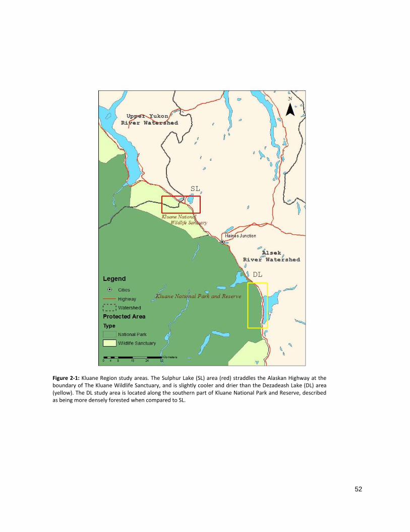
52
2.7 Figures and Tables
Figure 2-1: Kluane Region study areas. The Sulphur Lake (SL) area (red) straddles the Alaskan Highway at the boundary of The Kluane Wildlife Sanctuary, and is slightly cooler and drier than the Dezadeash Lake (DL) area (yellow). The DL study area is located along the southern part of Kluane National Park and Reserve, described as being more densely forested when compared to SL.
SL
DL
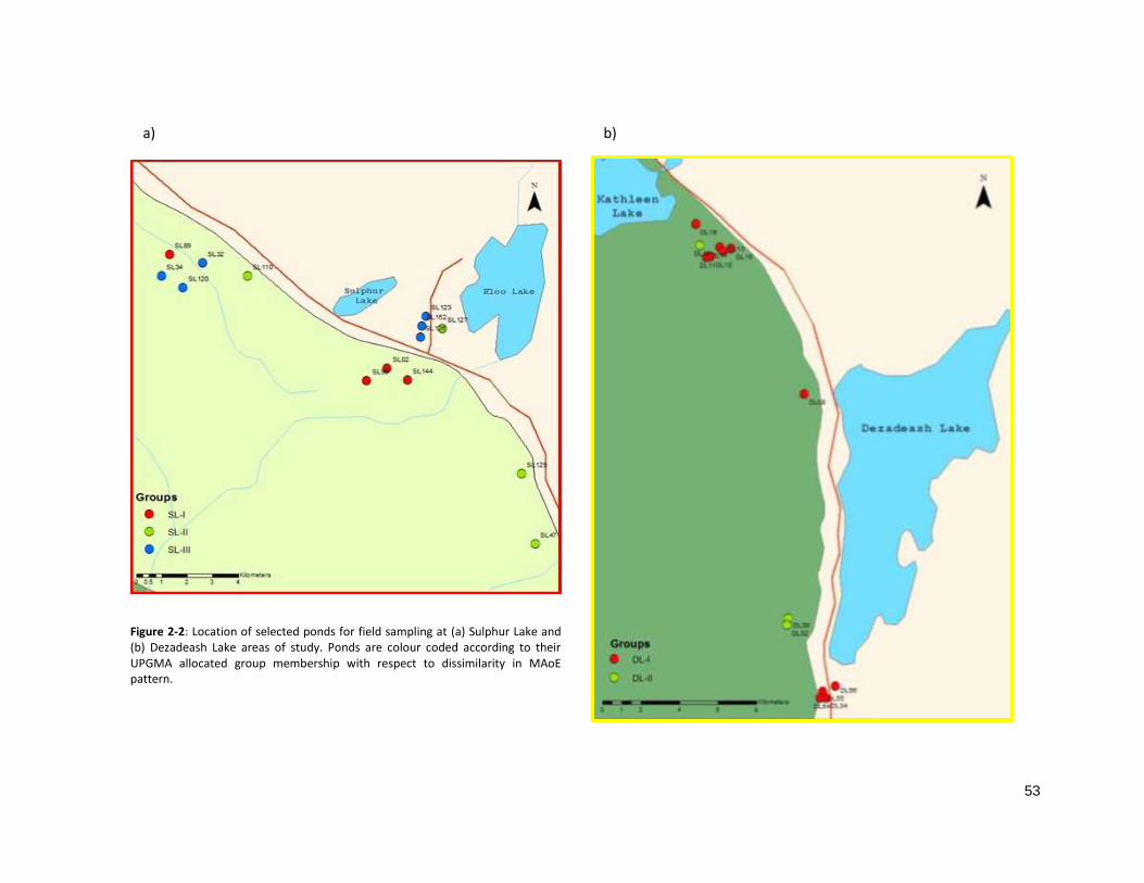
53
a) b)
Figure 2-2: Location of selected ponds for field sampling at (a) Sulphur Lake and (b) Dezadeash Lake areas of study. Ponds are colour coded according to their UPGMA allocated group membership with respect to dissimilarity in MAoE pattern.
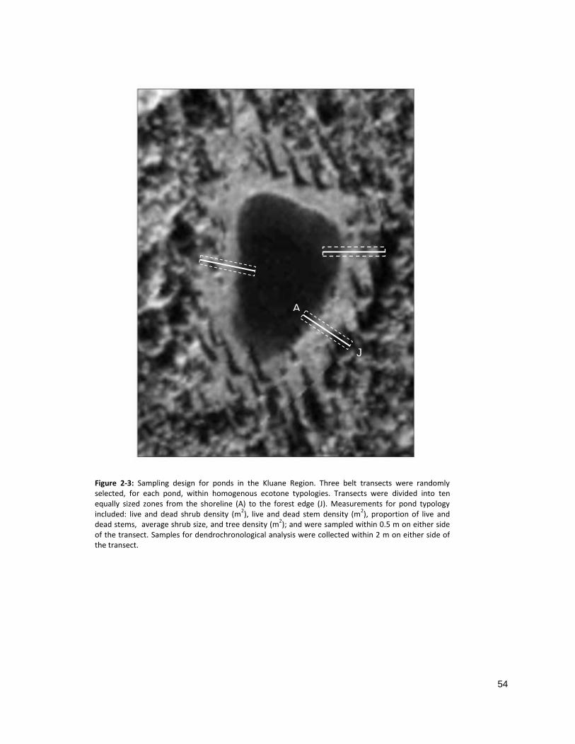
54
A J
Figure 2-3: Sampling design for ponds in the Kluane Region. Three belt transects were randomly selected, for each pond, within homogenous ecotone typologies. Transects were divided into ten equally sized zones from the shoreline (A) to the forest edge (J). Measurements for pond typology included: live and dead shrub density (m
2), live and dead stem density (m
2), proportion of live and
dead stems, average shrub size, and tree density (m2); and were sampled within 0.5 m on either side
of the transect. Samples for dendrochronological analysis were collected within 2 m on either side of the transect.
A
J

55
Interpretation of Results
Statistical objective
Identifying differences in
colonization rate
Similarity in Patterns of
Establishment
Dissimilarity Matrix
Correspondance Analysis
Determine χ2 distance between median MAoE of
zone and pond establishment pattern
Spatial dependence of MAoE patterns as determined by
zonal establishment characterisic of each pond
Multivariate Regression Tree (MRT)
Predict pattern in shrub establishment using average ecotone typology of ponds
Association between shrub colonization and ecotone
typology
UPGMA clustering (Groups)
Compare zone colonization between groups using mixed
effects modelling
Spatial heterogeneity of pond shoreline behaviour inferred
from colonization rates
Compare pond typology between groups using mixed
effects modelling
Potential hydrological influence over ecotone
characteristics (shrub density, height, mortality etc.)
Figure 2-4: Statistical design for MAoE analysis derived from dendrochronology data. The median age from all transects was selected as the MAoE for each zone within the pond ecotone. Analyses were performed using a dissimilarity matrix of median zone age of the three transects for each pond. Differences in MAoE pattern with respect to pond typology, were determined through MRT. Spatial similarities with respect to median zonal age were revealed by CA. Finally, ponds were allocated to clusters (groups) through a UPGMA dissimilarity matrix analysis based on MAoE by zone (associated with colonization rate). These groups were used to determine the statistical differences in colonization pattern and ecotone structure – a reflection of shoreline behaviour.
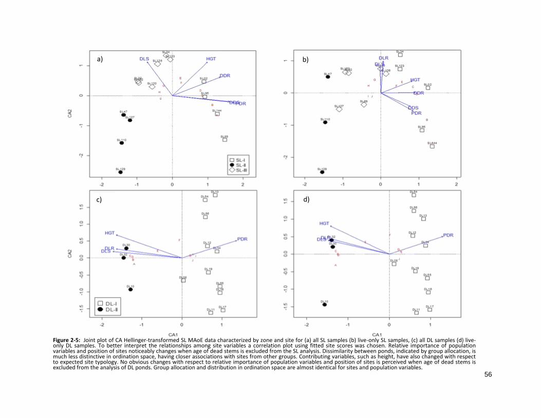
56
Figure 2-5: Joint plot of CA Hellinger-transformed SL MAoE data characterized by zone and site for (a) all SL samples (b) live-only SL samples, (c) all DL samples (d) live-only DL samples. To better interpret the relationships among site variables a correlation plot using fitted site scores was chosen. Relative importance of population variables and position of sites noticeably changes when age of dead stems is excluded from the SL analysis. Dissimilarity between ponds, indicated by group allocation, is much less distinctive in ordination space, having closer associations with sites from other groups. Contributing variables, such as height, have also changed with respect to expected site typology. No obvious changes with respect to relative importance of population variables and position of sites is perceived when age of dead stems is excluded from the analysis of DL ponds. Group allocation and distribution in ordination space are almost identical for sites and population variables.
a)
b)
c)
d)
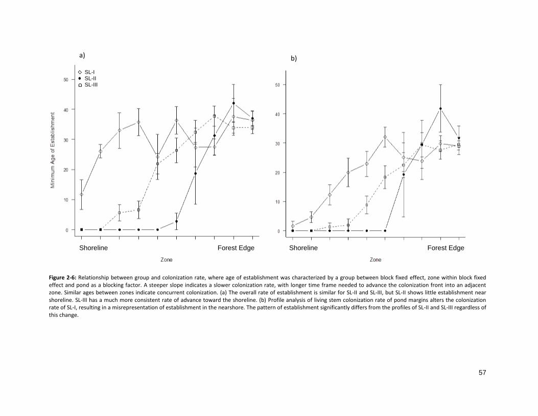
57
Figure 2-6: Relationship between group and colonization rate, where age of establishment was characterized by a group between block fixed effect, zone within block fixed effect and pond as a blocking factor. A steeper slope indicates a slower colonization rate, with longer time frame needed to advance the colonization front into an adjacent zone. Similar ages between zones indicate concurrent colonization. (a) The overall rate of establishment is similar for SL-II and SL-III, but SL-II shows little establishment near shoreline. SL-III has a much more consistent rate of advance toward the shoreline. (b) Profile analysis of living stem colonization rate of pond margins alters the colonization rate of SL-I, resulting in a misrepresentation of establishment in the nearshore. The pattern of establishment significantly differs from the profiles of SL-II and SL-III regardless of this change.
SL-I SL-II SL-III
a)
b)
Shoreline Forest Edge Shoreline Forest Edge
58
Figure 2-7: Relationship between group and colonization rate, where age of establishment was characterized by a group between block fixed effect, zone within block fixed effect and pond as a blocking factor. A steeper slope indicates a slower colonization rate, with longer time frame needed to advance the colonization front into an adjacent zone. Similar ages between zones indicate concurrent colonization. (a) Profile analysis of colonization rate shows that DL-I is much steeper from shoreline to edge of forest and differs significantly from the profile of DL-II. (b) Omitting dead samples altered the profile slightly, but rate and dependence on group interactions remains statistically similar.
DL-I DL-II
a)
b)
Shoreline Forest Edge Shoreline Forest Edge
59
Live
Ste
ms
(m-2
) %
Dea
d S
tem
s H
eigh
t (m
)
Shoreline Forest Edge Shoreline Forest Edge
a)
b)
c)
d)
e)
f)
Sulphur Lake Ponds Dezadeash Lake Ponds
Figure 2-8: Differences in community typology per zone with respect to: (a),(b) Live stem density; (c),(d) proportion of dead stems; and (e), (f) average height of individuals between pond groupings based on MAoE data.SL-I ponds are characterized by a more consistent shrub height across the ecotones with a much higher proportion of dead individuals in the near shore. DL-II ponds possess larger individuals on average, and a lower proportion of their stems are dead.
60
Table 2-1: Comparison of group and zone effect on ecotone shrub population structure for complete and living-only MAoE matrices in the SL study area. SL-II and SL-III typologies are compared to SL-I, where estimate is the unit change in population factor per increase increasing distance from shoreline, represented by zone.
* Significant value (p < 0.05)
Group Effect Zone Effect
MAoE Population structure
Group Estimate t-value Estimate t-value
Complete Non-living shrub
I 0.90 ±0.03 29.7152 -0.009 ±0.004* -2.282 II -0.19 ±0.04* -4.5367 0.009 ±0.006 1.614 III -0.19 ±0.04* -4.9065 0.009 ±0.005 1.746
Living shrub I 0.61 ±0.09 6.6049 0.044 ±0.013* 3.415 II -0.15 ±0.13 -1.1402 0.039 ±0.018* 2.131 III -0.05 ±0.12 -0.4437 0.047 ±0.017* 2.786
Non-living Stem I 1.39 ±0.25 5.5183 0.103 ±0.035* 2.918 II -1.09 ±0.36* -3.0486 0.036 ±0.050 0.719 III -1.01 ±0.33* -3.0967 0.083 ±0.046* 1.83
Proportion Dead Stem
I 116.74 ±7.58 15.4031 -6.69 ±0.993* -6.742 II -127.65 ±24.88* -5.1312 10.76 ±2.976* 3.617 III -93.32 ±13.54* -6.8908 7.05 ±1.713* 4.116
Height
I 0.89 ±0.06 15.6524 0.02 ±0.008* 2.649
II -0.32 ±0.08* -4.0232 0.03 ±0.011* 3.115
III -0.28 ±0.07* -3.8231 0.04 ±0.010* 3.863
Living Non-living shrub
I 0.81 ±0.04 21.7720 -0.0004 ±0.004 -0.1049 II -0.10 ±0.06 -1.656 0.0004 ±0.006 0.0642 III -0.05 ±0.05 -1.027 -0.005 ±0.005 -1.1280
Living shrub I 0.76 ±0.09 8.522 0.040 ±0.011* 3.5663 II -0.25 ±0.14 -1.7155 0.028 ±0.018 1.5240 III -0.37 ±0.12* -3.0290 0.072 ±0.015* 4.7611
Non-living Stem I 1.07 ±0.23 4.6639 0.151 ±0.032* 4.7234 II -0.74 ±0.37 -1.9773 -0.023 ±0.052 -0.4372 III -0.60 ±0.31 -1.9476 0.006 ±0.043 0.1525
Proportion Dead Stem
I 77.11 ±11.87 6.4952 -3.02 ±1.07* -2.8294 II -89.72 ±35.57* -2.5226 7.35 ±3.86 1.9065 III 10.44 ±18.79 0.5556 -4.22 ±1.84* -2.2907
Height
I 0.83 ±0.046 17.9417 0.035 ±0.007* 4.9415
II -0.29 ±0.076* -3.8136 0.026 ±0.012* 2.2281
III -0.22 ±0.063* -3.4465 0.013 ±0.010 1.3077
61
CHAPTER 3: VALIDATION OF MULTI-TEMPORAL REMOTE SENSING OF POND ECOTONES IN
SOUTHWEST YUKON USING DENDROCHRONOLOGY
3.1 Introduction
3.1.1 Inland water surface area decline in the North
Evidence for accelerated climate warming has been well documented in northern regions; where
ecosystems are characterized by both a high degree of sensitivity to external influence and isolation
from the direct anthropogenic disturbance typically experienced in the lower latitudes. The Arctic,
defined as regions north of 60° latitude, has experienced a reduction in sea-ice cover, a northward
retreat of permafrost boundaries, altered hydrological dynamics, and changes in biogeochemical
processes (Rouse et al., 1997; Serreze et al., 2000; ACIA, 2005; Hinzman et al., 2005; Myers-Smith et al.,
2011a). Observed shifts in Arctic surface water balance are expected to continue under a changing
climate (e.g. Rouse et al., 1997; Hinzman et al., 2005).
To date, changes in inland freshwater surface area in the Arctic have been studied largely via remote
sensing (e.g. Yoshikawa and Hinzman, 2003; Smith et al., 2005; Hinkel et al., 2007; Riordan et al., 2006)
or, in rare cases, decadal, systematic monitoring of freshwater ponds in the High Arctic (Smol and
Douglas, 2007). From these studies, several driving mechanisms of pond margin dynamics have been
reported, including changes to permafrost depth and extent in thermokarst regions (Hinzman et al.,
2005) and the intensification of potential evapotranspiration in high Arctic regions (Bring and Destouni,
2011; Carroll et al, 2011).
Although the observed net change in lake surface area has been spatially and temporally variable,
inland freshwater ponds in northern permafrost regions have generally experienced an overall decline in
recent decades, with potentially significant ecological effects. Areas showing the greatest declines are
those susceptible to drainage due to a deepening active layer (Yoshikawa and Hinzman, 2003; Riordan et
al., 2006), areas impacted by anthropogenic disturbance (Hinkel et al., 2007), or areas experiencing
62
increased evaporation rates with negligible changes in precipitation, resulting in a negative water
balance (Smol and Douglas, 2007; Abnizova and Young 2010). A decadal water surface area map of the
entire Canadian Arctic revealed a clustering of inland water bodies in decline throughout the northeast,
a concurrent net gain in the southwest, with a net loss in surface water overall (Carroll et al., 2011).
Research into the mechanism of net decline is a focal point of water resources research in the Arctic.
Increases in surface area, observed throughout the continuous permafrost zone in Russia using time
series remotely sensed data, were attributed to increasing thermokarst (Smith et al., 2005). A study of
change in continuous permafrost zones with the use of mid-resolution satellite imagery and historical
aerial photography by Riordan et al., (2006) found a spatially heterogeneous pattern of pond change in
sub-arctic Alaska, which was attributed to patchiness of processes affecting hydrology in the North.
These included thermokarst processes, presence of permafrost, soil desiccation and forest fire
dynamics. The observed overall trend in surface area decrease was attributed to warmer and longer
growing season over the period of study.
To explain these heterogeneous pond dynamics, Roach et al. (2010) compared the physical properties
of neighbouring closed-basin lakes in the Alaskan boreal region to characterize the underlying
mechanisms conducive to either a decreasing or nondecreasing surface area, including permafrost
stability, hydraulic gradients, and lake catchment topography. Primary drivers of lake area reduction
included terrestrialization and evapotranspiration, while thermokarst formation was typical of
nondecreasing lake area. These results are fundamentally based on changes in surface area acquired
from the multi-temporal remotely sensed time series by Riordan et al. (2006).
In the same region, higher resolution IKONOS imagery combined with ground penetrating radar used
by Yoshikawa and Hinzman (2003) revealed a more temporally dependent pattern of surface area
change, where pond increase and decrease resulted from successive stages in permafrost transition
driven by climate change. Thawing permafrost and a deepening active layer increased thermokarst

63
activity, first creating new ponds in newly formed depressions then subsequently draining through taliks
formed at the bottom of mature thermokarst ponds.
Documentation of changes in inland lake surface area is limited largely to either permafrost regions in
the High Arctic, or discontinuous permafrost regions of Alaska. In addition, these studies also rely
heavily on change detected through remote sensing. The reliance on repeat imagery makes conclusions
about the driving mechanisms of change speculative. For example, a general agreement as to the
increase in pond surface area due to talik formation is contradicted by direct high resolution monitoring
of High Arctic ponds underlain by granite in the Canadian Arctic (Smol and Douglas, 2007). Direct
measurement of water levels over a 24 year period revealed that previously stable High Arctic ponds
were decreasing in response to atmospheric conditions and not thermokarst processes. Although
distinct, these driving mechanisms are not mutually exclusive. The environmental conditions resulting in
pond expansion, such as permafrost degradation and thermokarst development, can rapidly transition
to decreasing surface area as a result of climate factors (Jorgensen and Shur, 2007; Skrinner and Boike,
2010). Unfortunately, the long term high resolution records required to elucidate patterns of this nature
are non-existent for most Arctic regions, making generalization impossible.
There are several reasons for the uncertainty in change detection based on remote sensing. For one,
the spatial resolution of most remotely sensed data in northern regions is less than ideal for the
delineation of small pond boundaries, thereby biasing assessment of water resources toward larger
lakes, and in practice, ignoring dynamics and processes of small ponds (Sannel and Brown, 2010) that
potentially play an important biogeochemical role in atmospheric and landscape processes (Chapin et al.
2000; Skrinner and Boike, 2010). Carroll et al. (2011) estimate that the majority of water bodies found in
Arctic regions are small (1 to 10 ha in size) and inaccessible, and are therefore not well documented in
maps or low resolution aerial photography. In the same study, the authors collected a series of daily
observations from MODIS data from 2000-2009 to create annual surface water maps. An analysis of

64
decadal change in surface water over the Arctic revealed that the greatest variability in net change
occurs with lakes smaller than 300 km2, the majority of which showed an overall net decrease in area of
nearly 6,700 km2. Due to the clustering of gains and losses, the changes in surface area across the
Canadian Arctic were attributed to the differences in terrain rather than the abundance of lakes in a
given region; with the High Arctic experiencing the most significant losses and the southwest
experiencing net gains.
The short time frame investigated by Carroll et al. (2011) demonstrates yet another issue with remote
sensing. Even with the advent of high-resolution imagery (pixel resolution lower than 1.0 m), and more
frequent image capture (the authors utilized daily observations from low resolution MODIS
instrumentation), they possess a shallow temporal depth due to the relatively recent introduction of
these orbital sensors, impeding the ability to make any definitive conclusions about the effect of climate
warming over the last few decades. While high resolution aerial photographs are available for historical
periods, they are spatially and temporally sporadic, particularly in remote regions such as the Canadian
Arctic, with researchers usually only able to obtain quality photographs for only a few years over a large
time span; and even then, only for a limited number of sites (e.g. Yoshikawa and Hinzman, 2003;
Riordan et al., 2006, Labrecque et al., 2009). As a result, any seasonal or short term variability occurring
between years is omitted. This paucity of remote sensing data in the Arctic makes inference about
climate response more difficult; especially due to the natural variability of climate regimes in the North.
3.1.2 Validating change detection of multi-temporal remote sensing with dendrochronology
Dendrochronology is a well-established technique for quantifying natural processes and human
caused environmental events through the physical or chemical properties of tree ring structure or the
dating of tree ring formation (Speer, 2010). The processes involved in tree growth and ring formation
capture natural historical records conducive to the characterization of past climatic conditions,

65
disturbance regimes, community structure and migration, geophysical processes and a number of
temporally dependent phenomena of interest to landscape ecologists. In the current study, a
chronology for the advance of a colonization front within the pond margin ecotone is used as a proxy for
decadal changes of small pond shorelines in the southwest Yukon.
The impacts of natural disturbances can be preserved in growth-ring records, allowing for near annual
resolution of past events (Gottesfeld and Gottesfeld, 1990; St. George and Nielsen, 2003; Stoffel and
Beniston, 2006; Ballesteros et al., 2010ab; Ruiz-Villanueva et al., 2010). Typically used in fluvial
geomorphology, the principles of dendrohydrology have allowed for the successful reconstruction of a
number of natural hydrological processes. For instance, dendrochronologists have been able to exploit a
broad range of physical evidence preserved in tree rings to develop insights into the occurrence, extent
and magnitude of floods prior to available direct observations (St. George, 2010). Tree scars in the
growth ring record have been suitable paleo-channel roughness indicators in estimating past flood
discharge or magnitude (Stoffel, 2010; Ballesteros et al., 2011a). Analysis of rings has been successful in
indicating paleo-stage height and in the calibration of floodplain roughness (Balleresteros et al., 2011b),
as well as the timing of ice flow and flood events (Lepage and Bégin, 1996; Bégin and Payette, 1991;
Tardif and Bergeron, 1997) and minimum elevation of flooding events from high scar marks (St. George,
2002). St. George (2010) argued the benefits of using dendrochronological methods, asserting that they
have a high temporal resolution and dating accuracy compared to most other methods. In flood studies,
these methods are reported to have routinely dated past floods to the year of occurrence and, in rare
cases, can estimate the timing of floods that occur during the growing season to within two weeks;
chronological resolutions that are surpassed only by direct observation or instrumentation.
Successful dating of water level fluctuation and flooding events, using associations between ring
formation and width in response to hydrological dynamics, depends largely on the scale and physical
processes of the hydrological system under study. These systems are either fluvial in nature or large

66
enough that wave erosion provides the energy needed to force debris and ice past robust riparian
vegetation with enough force to damage the bark but not kill the tree during high water level rise.
Additionally, lake studies are on such a large scale that changes are gradual and can be tracked with
well-studied tree species, with well-established chronologies or a capacity for cross-dating. Sample
depth is typically longer, allowing for the development of long term chronologies, tracking
geomorphological changes back centuries.
The same principles can be applied on a much smaller scale to the retreat of pond shorelines using
the timing of vegetation establishment, instead of ring associations with hydrological processes. The
establishment of an individual signifies the retreat of the pond margin, analogous to the removal of a
‘barrier effect’, allowing for vegetation to grow in the newly exposed pond margin. The short timescale
and small spatial scale of pond surface dynamics make ring-width indicators and tree-ring chronologies
impractical for this study. The species under analysis must adhere to a number of criteria to make any
plausible inferences about the timing of pond margin recession. The species must: (1) rapidly colonize
suitable sites as they become available in order to minimize ecesis and maximize chronological
resolution shoreline dynamics; (2) be moisture adapted to ensure successful establishment and to avoid
confounding interactions stemming from interspecies competition at the pond edge; (3) possess a large
enough population pool in the surrounding forest ecosystem; and 4) display an upright growth form
with clearly discernible annual rings for accurate ring counting and cross dating. Although there are
several species that fit almost all of this criteria, those belonging to the genus Salix seem to be the most
tolerant of moist conditions, and are usually the primary establishers in the water catchment zone
(personal observation, 2011). Salix spp. have also been used successfully to date the timing of ice-push
in Northern Quebec (Bégin and Payette, 1991), displaying a typical annual ring growth pattern.

67
3.1.3 Objectives
The association between pond water levels and surrounding vegetation has the potential to elucidate
decadal dynamics of shoreline behaviour, made necessary due to the variability in hydrological regime,
heterogeneity of northern landscapes and the lack of direct observation and measurement data
available for Arctic regions. Dendrochronological analysis of woody vegetation produces high
chronological resolutions with which to validate changes in surface area determined through low
frequency multi-temporal remotely sensed imagery. Researchers investigating dynamics of northern
ecotones have used dendrochronology to date periods of shrub and tree encroachment into previously
herbaceous ecotypes (e.g. Danby and Hik, 2007; Myers-Smith et al., 2011a). The current study employs a
similar approach to date the colonization of recently exposed pond ecotone areas by shrubs and trees to
develop a chronosequence of water level behaviour. The intent of this study was to investigate the
association of remote sensing techniques and dendrochronological analysis in a northern context for the
purpose of validating changes measured through multi-temporal remote sensing time series.
It was hypothesized that the accuracy of pond margin change detection would be improved by
supplementing remote sensing with dendrochronology to date periods of shrub and tree establishment
in pond ecotones. Remote sensing techniques will allow for a broad scale assessment of overall change
in sub-Arctic ponds, while dendrochronological techniques will provide evidence for the accuracy of
trends identified by aerial photographs and satellite imagery on a finer scale. Integration of the two
techniques and comparison with meteorological records will allow for the evaluation of connections
between changes in regional climate and surface hydrology over the past 60 years.
The diverse landscape and climate regime of the Kluane region of the southwest Yukon was well
suited to objectives of this study: a sub-Arctic boreal ecosystem underlain by scattered discontinuous
permafrost, characterized by variable terrain and spatially distinct climate regimes. These environmental
conditions are less substantially quantified in terms of pond surface area dynamics, and exhibit
characteristics similar to inland freshwater bodies found in previous studies. The Kluane Region has also
68
experienced some of the most significant climate warming in the North over the last 40 years. The
majority of ponds in the Yukon are shallow open water ponds, represented by those in the current
study, which are most susceptible to small changes in environmental conditions (Carroll et al., 2011).
3.2 Methods
3.2.1 Region of study
The Kluane National Park and Reserve and the Kluane Wildlife Sanctuary are located in the southwest
corner of the Yukon. Generalizations about climate in the Kluane Region are difficult due to the diverse
topography which produces highly variable wind patterns, solar radiation availability, and moisture
regimes within short distances (Gray, 1987). However, there are distinct north-south transitions, as well
as maritime-continental climatic divides. At the northern end, in the Donjek Valley, the moisture regime
is dry, temperatures are lower, and the soil is underlain by discontinuous permafrost. In the south,
climate is warmer and moister with greater soil development, and denser forests and wetland
vegetation.
Wetlands are generally associated with major lakes in the ecoregion which include Kluane, Dezadeash,
Kathleen, Mush and Bates Lakes. These lakes are supplied and drained by extensive fluvial systems. This
region has been inundated several times over the past few hundred years as a result of glacial blockages
across the Alsek River (Yukon Ecoregions Working Group, 2004). Relative to other areas in the Arctic, the
Yukon does not possess extensive systems of wetlands. Instead, wetlands cover less than 5% of the
Territory and are composed largely of shallow open water ponds.
The two study areas are located in the Ruby Ranges ecoregion (Fig 3-1); one of the driest regions in
the Territory due to its geographic location in the rain shadow of the St Elias Mountains (Gray, 1987).
The nearest weather station is located in the town of Haines Junction, equidistant between the two
areas. Average monthly temperature and total precipitation for Haines Junction are presented for the
period 1945-2006 (Fig 3-2). The majority of ponds in study areas are found within the Aishihik Basin
69
which is drained by the Alsek River, comprising 4% (19,000 km2) of the Territory (Janowics, 2004). Ponds
of interest are scattered along the Shakwak Trench in the region southeast of Kluane Lake; falling within
the sporadic discontinuous permafrost zone. Permafrost near Haines Junction has been recorded at 7.3
m but most of the ground is only seasonally frozen (Yukon Ecoregions Working Group, 2004).
3.2.2 Pond selection
The study area was subdivided into two regions to account for a north-south climate gradient,
referred to as the Sulphur Lake (SL) and Dezadeash Lake (DL) areas (Fig 3-1). An inventory of all potential
ponds in each region was generated using NTS map sheets and Google Earth v.6.1.0.5001 imagery
(Google Inc., 2011). Suitable ponds were selected based on a set of criteria that would control for the
influence of geomorphic and topographical factors while maximizing the number of ponds that could be
sampled in the field. Potential inclusion of each pond in field sampling was based on a subsequent set of
criteria intended to evaluate patterns of shrub establishment that accurately represented shoreline
dynamics which were comparable across both study areas.
First, a symmetrical shape was considered; with desirable ponds possessing a length-to-width ratio
close to 1:1. Ponds that deviate from a circular shape are more likely to be bathymetrically
asymmetrical, resulting in dissimilar environmental gradients depending of the aspect sampled; which in
turn results in a variable vegetation structure and ecesis. Second, any edge effects from secondary roads
and the Alaska Highway, or from forest clearing for the pipeline right-of-way, may also impact the
establishment, survival, and age structure of surrounding vegetation (see Harper et al., 2005). To
mitigate edge effects of this nature, ponds which were isolated from anthropogenic disturbance were
desirable; however, ponds still needed to be accessible on foot from the Alaska Highway. Finally, the
assessment of potential effects of climate on shoreline was facilitated by restricting pond analysis to
closed-basin ponds. Closed-basin ponds are defined as having no visible surface connection to nearby

70
fluvial systems. This characteristic facilitates the isolation of climate forcing with respect to the
precipitation-evaporation ratio, evapotranspiration, and permafrost dynamics (Anderson et al., 2007;
Abnizova and Young, 2009; Roach et al., 2011). This restriction was necessary in order to reduce
confounding seasonal variability resulting from natural fluctuation in fluvial systems including the Alsek,
Jarvis, and Dezadeash Rivers.
Once all suitable ponds were identified, fourteen from each study area were then randomly selected
for analysis and sampled in the field. A minimum impact philosophy was used to guide all field related
activities and Parks Canada’s protocol for scientific field work was followed at all sites. Unnecessary
trampling of vegetation and wildlife disturbance was minimized. Because anurans are particularly
susceptible to Chytridiomycota, boots were rinsed in a diluted bleach solution prior to pond visitation to
prevent the introduction of the fungus into the National Park. In addition, noise was kept to a minimum
when sampling at ponds where the presence of waterfowl was evident, and the nest sites of wetland
species, such as trumpeter swans, and wood frog egg masses were avoided.
To improve the scope of surface area change in the Kluane Region, an additional 6 ponds for each
study area were included in the remote sensing change detection analysis, yielding a total of 20 ponds in
both areas for each time interval (Fig 3-3). These supplementary ponds were selected based on similar
criteria to field selection.
3.2.3 Image analysis
Ponds were identified in three equally spaced time steps represented by both historical aerial
photographs, and high resolution satellite imagery, including repeat panchromatic imagery from
baseline in 1940s (AP40), mid-series imagery from the 1970s (AP70), and recent QuickBird imagery (QB).
Aerial photographs of the Alaska Highway, edging Kluane National Park and Reserve and the Kluane
Wildlife Sanctuary, were obtained from the National Air Photo Library, Ottawa, ON. Photographs were

71
first evaluated visually for location and clarity then requested in digital form (Table 3-1). Contact prints
were scanned by NAPL at a resolution of 1200 dpi (between 0.85 m to 1.69 m pixel resolution). All
historical aerial photographs were acquired in 1948, in either late June or early July, at an altitude of
20,000 ft. a.s.l. The mid-series aerial photographs were acquired during the mid-1970s in July to early
August. Image selection was based on the proximity of the ponds to the center of the photograph in
order to reduce the internal geometric error inherit in airborne data acquisition off the principle point.
A higher spatial resolution was chosen over higher spectral resolution when assessing current pond
surface area for SL and DL (see Appendix D for details). One ortho-ready, radiometrically corrected
panchromatic QuickBird image (QB) for each of the SL and DL study areas was obtained from
DigitalGlobe Inc. The images were acquired June 14, 2008 and June 25, 2011 respectively. The ponds
were within 25° off-nadir, recording surface features at a 0.61 m pixel resolution. The QB image was
rectified in Geomatica Focus version 10.3 (PCI Geomatics, Toronto, ON), using the associated rational
polynomial coefficients (RPC) obtained from DigitalGlobe Inc. and a 30 m digital elevation model (DEM)
obtained from the Government of Yukon, Department of Energy and Mines. It was important that the
timing of image acquisition was coordinated as best as possible between the aerial photographs and the
satellite image for each region to avoid discrepancies resulting from short term, seasonal variations in
climate.
3.2.3.1 Image-to-image registration
A hybrid approach was utilized to register images to ground coordinates. First, the QuickBird images
were rectified to accurate ground UTM coordinates and then the aerial photographs were registered
and georeferenced to the QB image at 0.61 pixel resolution. Image-to-image registration was chosen for
AP40 and AP70 to facilitate a correspondence of ecotones across the time series. This approach was
more practical for the purposes of this study as unique x, y coordinates for each pixel would not be as
72
informative for time series analysis. This technique is also conducive to the accurate detection of
changes in pond surface area over the current time series, as consistent placement of ground control
points (GCP) across the images is promoted. In addition, error from third party image rectification is
reduced along with distortion in feature geometry incurred from the acquisition process (Jensen, 2007),
which would produce poor comparability across the time series.
Each scene was selected based on: (1) ease of object identification in each photograph to reduce
uncertainty in identifying GCPs; (2) stability over time, to reduce potential error in registering images
based on features which may have changed over the course of the time series (i.e., flow pattern of
fluvial systems across the landscape); and (3) relatively uniform topography, away from the St. Elias
Mountains. Although DEM data was integrated into the rectification of the QB images, the topography
adjacent to the Alaska Highway, particularly around the Dezadeash Lake Region, consists largely of steep
relief due to the St. Elias Mountains, resulting in highly variable elevation across the landscape. A brief
description of GCP selection and image registration is provided in Appendix C.
To maximize accuracy with respect to pond shoreline, GCPs were restricted to low lying areas with
even topography (Hughes et al., 2006). There was a lack of hard classifiers in the images and solitary
trees and rock outcrops were used almost exclusively for GCPs. Accuracy is critical in change detection
analysis, and challenging given the low quality of historical images. Therefore, for each area of interest,
at least one GCP was established for every square kilometer of the area containing sampled ponds.
Images were rectified using a second-order polynomial, due to the variability in terrain, with an RMSE
less than 1.2 m. A cubic convolution resampling method was applied to the panchromatic aerial
photographs prior to manual delineation to facilitate the manual digitization of natural boundaries
(Hughes et al., 2006; Sannel and Brown, 2010) (Fig C-1).

73
3.2.3.2 Manual delineation and pond classification
To detect patterns of change in surface hydrology over the last 60 years, the surface area of all small
ponds (<0.05 km2) found in AP40 photos were measured as a baseline for subsequent change. Pond
surface area, defined as area of open water within the aquatic-terrestrial ecotone transition, was
measured by manually digitizing the shoreline separating the surface area of open water from upland
terrestrial vegetation. Shoreline was defined as the point where open water transitioned to emergent
vegetation, which proved to be well defined in remotely sensed imagery and in the majority of field
sampled ponds. Large islands of emergent vegetation were also digitized, and were excluded from total
surface area.
Manual delineation depends greatly on the discretion of the interpreter, especially with small scale
images. Several procedures were utilized to improve digitization accuracy, and are outlined in Appendix
D. Due to the utility of binary encoding analysis for identifying pond boundaries, this technique, as
described by Sannel and Brown (2010) using ENVI Image Analysis Software v.4.0 (Exelis Visual
Information Solutions, Boulder, CO), was adopted for the lower quality aerial photographs to aid in the
detection of open water shoreline required for manual delineation. Details on the execution and
assumptions of this method can also be found in Appendix D. To account for the potential uncertainty
resulting from human decision making in distinguishing shoreline from changes in terrestrial community,
ten delineation trials for each pond sampled in the field were performed and the uncertainty,
represented by the standard error of the mean surface area, was calculated for each.
3.2.3.3 Quantification of lake dynamics
Binary encoding profiles were created for each pond in the aerial photographs. One profile was
created for every 25-50 m of shoreline, depending on how distinct the shoreline appeared in the image,
to use as a reference for assessing shoreline (Fig D-1). The surface area measurements were calculated
in ESRI® ArcMap 10.0 (ESRI, Redlands, CA) from polygons created during the delineation process. The

74
number of vertices created, relative to area measured, was also calculated for each polygon to compare
the precision associated with each image. The net gain or loss of surface area detected from the
historical aerial photography to the recent aerial photography was quantified by measuring change in
open water surface area. Using the historical surface area as a baseline, the amount of change in pond
surface area was determined by calculating the percent increase or decrease in surface area measured
in AP70 and QB images using the time series data collected from the remote imagery.
3.2.4 Assessing shrub minimum age of establishment (MAoE)
In this study, the pond ecotone was defined as the area of vegetation spanning the shoreline to forest
edge, as this community has most likely been influenced by the hydrological regime of the pond. The
forest edge was defined as the zone in which the vegetation community transitioned to spruce-
dominated forest. In cases where this transition was unclear, or at uninformative distances, a significant
change in slope, where an obvious levelling of relief occurred, was taken as the perceptible limit of
former pond bathymetry. In the majority of cases these criteria corresponded quite well.
At each pond, the ecotone was divided into three areas of similar population structure. A transect
was established randomly within each area, perpendicular to shoreline and spanning the entire ecotone
(Fig 3-4). Homogenous growing conditions were chosen for transect placement in order to minimize
potential zonation resulting from variability in horizontal environmental gradients (Bendix, 1994), rather
than the succession of plant establishment as a result of retreating shoreline (Bégin, 1989). Because the
degree of slope from forest edge to shoreline plays a role in hydrological regime, a major factor in
determining establishment of surrounding terrestrial vegetation (Strayer and Findlay, 2010), the slope of
all pond margins was kept consistent between transects and ponds.
In some cases it was not possible to begin each transect at the pond shoreline. This included ponds
SL-144 and SL-152, which were too deep to access, and the shoreline of DL-08 which was more than 50

75
meters from the furthest shrub establishment in relation to the forest edge. In these cases, transects
were established from the forest edge toward open water for a maximum distance of 30 meters.
Although this could potentially influence the pattern of minimum age of establishment across the zones
in each of these ponds, the high water levels suggest that woody vegetation would have been unable to
establish successfully in these areas.
3.2.4.1 Dendrochronological Sampling
The dendrochronological response of shrubs may differ significantly by taxa, therefore only the
dominant genus was chosen for the current study. Salix spp. were clearly the dominant shrub type at all
but the two higher elevation ponds (> 1000 a.s.l.), and was therefore chosen for sampling across the
entire region. Salix spp., in particular, are prominent tall shrubs on the landscape that are well suited to
moist soil environments and are likely to minimize ecesis, establishing much more rapidly than either
spruce or other shrub species. Sampling was also restricted to tall Salix spp., to minimize issues related
to compact and uninformative ring formation (Schweingruber et al., 2011). For the collection of
dendrochronological samples, transects were divided longitudinally into ten, equally sized, zones of
establishment that were two meters wide on either side of the transect (Fig 3-4). In this way, the size of
each zone was relative to the length of the transect, allowing for inter and intra-pond comparison of
transects.
In order to determine absolute date of establishment, and account for irregular or missing rings,
the entire root collar must be extracted and each stem serial sectioned in accordance with Kolishchuk
(1990) to properly age each stem. Even then, the determined age indicates the absolute age of the
clone, and not necessarily the parent individual. These methods are time consuming, and would result in
a reduction of sample size. In addition, resources required to sample each individual at the cormus, for a
study of this size, are not practically available, nor would the destructive nature of this form of
76
dendrochronological sampling be acceptable within national park boundaries. A more practical
approach was taken to estimate the timing of shoreline retreat. Assuming that the largest central stem
is the dominant and therefore earliest growing stem, one section was collected for analysis from the
three largest live basal stems in each zone. Sections were taken as close to the true root collar as
possible. Because willows typically establish by seed on moist substrate (Bégin and Filion, 1995), each
group is likely a genetically identical individual. The age of each genetic individual corresponds to the
earliest date at which a given site in the pond ecotone was made available for establishment. Since we
are simply interested in the relative ages of establishment, to develop a pattern of shoreline
colonization with which to compare with directional changes in remote sensing, a trade-off between the
sample size of individual shrubs and stem sections and the number of ponds sampled was considered
acceptable.
3.2.4.2 Dendrochronological Analysis
Sample sections were progressively sanded down to a grit level of 600, and then ring width time
series were measured to the nearest 0.001 mm using a Velmex “TA” system (Velmex Inc., Bloomfield,
NY) in conjunction with the MeasureJ2X software v.4.1.2 (VoorTech Consulting, Holderness, NH). The
diameter of each section was measured and sample age was evaluated for each stem. The average age
of the oldest stem was significantly older than the average of the youngest stem in each zone, validating
our assumption that dominant stems are typically older. In addition, the odds of the smallest stem
being the oldest decreased by a factor of 0.65 when compared to any other size, providing some
evidence that a sample of the three largest stems likely captures the minimum age of establishment for
that zone.
A chronological profile was then generated for each transect from the water surface edge to the
upland forest edge for each pond margin. Larger sections with clearly defined rings were used to create
77
master ring width chronologies for each pond. Master chronologies were validated using the software
COFECHA version 6.06 (Holmes, 1983) to the point where recommended shifts in flagged sections did
not significantly increase the correlation among sample chronologies. The limitation in sample depth
(i.e. the average age of the shrub population) made this necessary, as COFECHA cannot adequately
validate samples younger than about 60 years. Because the average sample depth was less than 60
years, validating time series with younger samples would potentially result in spuriously high or low
correlations (Grissino-Mayer, 2001).
The remaining samples were cross-dated visually and correlated in accordance with COFECHA
software, where a Pearson’s correlation coefficient of 0.42 was the minimum value necessary to be
considered well correlated. Adding missing rings and removing potentially false rings was avoided unless
the change visually improved or significantly changed sample correlation with the master chronology.
The number of false or missing rings was minimal when samples were visually cross-dated with the
master sequence of large shrub sections possessing distinct marker rings. The observation of few
missing and false rings within shrub sections is consistent with other dendrochronological studies
utilizing shrubs (Bégin and Payette, 1991; Von Mörs and Bégin, 1993; Bégin and Filion, 1995). Confidence
in the accuracy of MAoE is corroborated by the significantly older age of stems which cross-dated
visually, and correlated well with master chronologies than those that cross -dated poorly (1.34 ±0.63
years, t = 2.13, p < 0.05, and 8.4558 ±0.77 years, t = 10.95, p < 0.001, respectively). Samples that
correlated well were also likely to be visually well cross-dated with odds decreasing by a factor of 4.48
when not well correlated. The age corresponding to the oldest of the sampled stems was taken as the
minimum age of first establishment (MAoE) for each plot.

78
3.2.4.3 Seasonal variability and evaluation of dead samples
The possibility remains that water levels may fluctuate over longer time periods than experienced
through seasonal variability, or have remained consistently low over time periods exceeding average
shrub age. In large-scale systems, with well developed, or mature, shrub margins, true age is critical for
estimating fluctuations in unstable shorelines. Bégin and Filion (1995) performed a metapopulation
analysis of shoots in order to characterize shrub survivorship under periods of high water events.
However, this was not practical with the number of ponds selected for the study. Instead, large dead
stems (in addition to the live samples) from each zone were sampled as a surrogate, under the
assumption that the death of individuals within multiple zones would coincide if the cause of mortality
were long periods of high water levels. The number of dead stems reflected the proportion of dead
individuals found at each site. The same criteria for live stem selection, sample processing, and
dendrochronological analysis was applied to dead stems.
3.2.5 Statistical Analysis
The aim of this study was to quantify changes in pond surface area using remotely sensed time series
data and validate these shoreline dynamics using timing of shrub MAoE from forest edge to shoreline.
The spatial profiles of shrub chronologies represent the rate of colonization from forest edge to open
water, as the shoreline position changes over time. Shoreline behavior may vary spatially, subject to
unknown hydrological associations. If shrub establishment is associated with changes in shoreline
position, combining the MAoE data for all ponds would have masked these differences. Therefore,
ponds were first grouped by similar patterns in shrub MAoE to identify these potentially divergent
hydrological regimes. The subdivision of ponds based on MAoE reflects differences in colonization rate
from forest edge to pond shoreline, and can be compared statistically in order to verify differences in
water level dynamics across the Region. Ponds were also subdivided by study area, as moisture regimes
79
vary between the SL and DL sample areas, potentially resulting in distinct shoreline dynamics and
colonization patterns.
The overall approach to data analysis for this study is outlined in Figure 3-5. Surface area for each
pond was measured for images representing each time period (AP40, AP70, and QB) from which the
direction of change from baseline could be determined. The association of shrub establishment and
shoreline behaviour was then assessed by comparing change in surface area between groups displaying
distinct establishment patterns. The rate of colonization was determined by calculating the distance of
shrub colonization front from the forest edge for years represented by AP40, AP70, and QB. Finally,
change in surface area from baseline to AP70 and QB was validated by comparing position of shrub
colonization fronts for years represented by remote sensing data.
Although the analysis of transects would increase the sample size considerably, each pond was
considered a sampling unit in all analyses in order to reduce the inevitable pseudoreplication resulting
from inter-pond correlation of colonization patterns. Minimum age of establishment per zone was
defined by zonal median age between all three transects. Median age was used to preserve the
character of real age data and to avoid under or over estimation of first establishment due to chance
survival or mortality of shrubs in the sampled zone.
All statistical analyses were performed with the open source statistical software R version 2.14.1 (R
Development Core Team, 2011). The vegan package (Oksanen et al., 2012) was used for cluster analysis
and the nlme package (Pinheiro et al., 2011) was used for all mixed linear modeling. Data structure was
assessed for normality and equal variance prior to analysis. Normality and structure of residuals were
evaluated for fulfillment of assumptions of equal variance and normal distribution of residuals.

80
3.2.5.1 Change in pond surface area over time
Change in surface area was assessed by calculating absolute changes in surface area across the
landscape (m2 lost or gained), in addition to the relative change in each pond by comparing the
standardized change in surface area for each pond. Potential error introduced as a result of image
quality, not reflective of actual surface area change over time, was also evaluated due to the significant
disparity in shoreline clarity between the three time periods (Fig 3-6). To evaluate changes in precision
between image types, the number of vertices per m2 was quantified and compared using a Bartlett test
of equal variances. Average m2/vertex increases slightly with image quality (Fig D-2), but this change was
insignificant. Although variation in pond size is expected to change between years across the region, if
accuracy is comparable despite image type, variation in trial sizes should be kept constant between
images for each pond (Tables 3-2 and 3-3). Consistency in trial delineations is a reflection of accuracy,
and was also compared between image types using a Bartlett test (Table 3-2 and 3-3). Variance was
unequal for surface area measurements for different image quality for all ponds (Bartlett's K2 = 41.23, df
= 2, p-value < 0.001) and within study areas (SL: Bartlett's K2 = 11.89, df = 2, p-value < 0.01; DL: Bartlett's
K2 = 37.72, df = 2, p-value < 0.001). This disparity in consistency reflects the difficulty in discerning
shoreline in lower quality images, therefore results should be interpreted at the discretion of the
researcher.
3.2.5.2 Differences in colonization rate and change in pond surface area
Shrub age data was analyzed with the purpose of identifying ponds with similar pattern in shrub
establishment through time. Shrub establishment reflects differences in shoreline behaviour, which can
be approximated using multi-temporal remotely sensed imagery. A Hellinger dissimilarity analysis,
typically used to assess the differences in sites with respect the abundance of species found at each site,
was used to determine dissimilarity between ponds based on the Euclidean distance of MAoE for each
zone. An Unweighted Pair-Group Method using arithmetic averages clustering method (UPGMA) was

81
then used to classify the ponds based on Euclidean distance of MAoE within zones. The UPGMA method
minimized average distance of dissimilarity between ponds and correlated highest with the original
Hellinger dissimilarity matrix.
The colonization rate of a pond margin, measured by the timing of establishment from forest edge to
shoreline, was compared with the overall change in waterline retreat previously identified by the
coarser-scale remote sensing. Direct comparison of water level change with colonization rates is
impossible, due to the low temporal resolution of the remotely sensed data in the Arctic region.
Although not ideal, another alternative is to reduce the resolution of dendrochronological data to match
that of the remotely sensed data. A coarse resolution colonization timeline was created by which the
position of the colonization front within the pond ecotone was determined for each year represented in
the multi-temporal image series. This colonization timeline was correlated with surface area
measurements from the remote sensing timeline. Comparisons between classes of colonization rates
and change in pond surface area measured through time series imagery were evaluated by mixed
effects modelling.
3.2.5.3 Climate data
To evaluate the potential use of these ecotones as indicators of climate change, surface change
chronologies constructed from the two techniques were compared with meteorological records in order
to assess the connection between climate variability and pond margin ecotone dynamics. Daily historical
climate data for the two study areas was acquired from Environment Canada spanning the last 66 years.
The nearest weather station is located in the village of Haines Junction, YT (60°45′10″ N, 137°30′24″ W),
approximately 50 km from the furthest pond sampled in both study areas. Because a significant portion
of climate data is missing, climate data was supplemented by data from nearby weather stations,
including Burwash Landing (61°21’11’’N, 138°59′12’’ W) and the City of Whitehorse climate stations
82
(60°43′0’’ N, 135°03′0’’ W) to create a more comprehensive timeline. Complete precipitation data was
obtained from Whitehorse, and temperature measurements from both nearby stations were used to
interpolate missing climatic values for Haines Junction. For details on this analysis refer to Appendix F.
Divergence in climatic conditions for years represented by the available imagery were compared to
the baseline conditions in 1948 in order to explain trends, if any, with changes in open water surface
area for the dates in question. Because images were acquired in the summer, a year was defined by
averages for fall and winter from the calendar year prior to image acquisition followed by spring and
summer climate for the corresponding year (Fig F-1).
3.3 Results
3.3.1 Change in surface area from remote sensing data
Changes measured from available remote sensing imagery are summarized for each pond in Tables 3-
2 and 3-3. Direction, or extent, of surface area change did not depend on the initial size of the pond
measured at either SL (AP70: F1,18 = 0.010, r2=0.001, p = 0.92, QB: F1,18 = 0.88, r2=0.044, p = 0.4) or DL
study areas (AP70: F1,18 = 0.034, r2=0.002, p = 0.8, QB: F1,18 = 0.049, r2=0.003, p = 0.8). Several ponds in
the DL study area have experienced an almost complete loss of open water, which was confirmed in the
field (Fig 3-7). More than half of all ponds measured in the DL area declined in surface area, nine of
which declined by more than 50% of their original size. Several supplementary ponds (D03, D05, D06)
along with the two high elevation ponds (DL30 and DL32, >1000 m a.s.l.), experienced a noticeable
increase in surface area over the latter half of the timeline. Ponds in the DL area declined by 17.31%
from 1948 to 1978, and continued to decline into 2011, with a reduction of almost 20 000 m2. This
represents a surface area decline of almost 40%, in sample ponds, since 1948. The total loss of surface
area for ponds analyzed in the SL area ponds was 26 000m2 greater than the total area lost from ponds
sampled at DL, but the relative decline was much less, declining by only 19% overall compared to the
40% loss at Dezadeash Lake.
83
The greatest losses were experienced at different stages in the time series between sample areas.
Highest measured losses in the SL area occurred from AP40 to AP70. The decline in surface area from
AP40 to QB was actually smaller than the previous time period, indicating a gain in surface area in recent
decades. Ponds measured in the DL area experienced similar declines in surface area for the first half of
the time series, but continued to decline into recent decades. The combined losses of all ponds sampled
in the Kluane region was 45 000 m2, a total of 24% of the surface area measured in 1948. The majority of
this loss occurred between the 1940s and 1970s, with further, though much smaller decreases over the
last 35 years. Linear mixed models reveal the overall decline in standardized surface area was significant.
The overall change in surface area from baseline was not significantly different between the two study
areas for either time period (Table 3-4).
Figures 3-8 and 3-9 show the spatial distribution of surface area changes in each area, from the AP40
to the AP70 and QB images. No discernible spatial patterns emerge in the SL area, although shoreline
expansion from 1948 occurred almost exclusively in the latter half of the study period; including all three
of the ponds south of Kloo Lake (Fig 3-8b). Almost every pond elsewhere in the region typically
continued to decline in the most recent time period. Most high elevation ponds, and those at the
southern end of Dezadeash Lake, remained stable or increased in surface area from 1948 baseline
measurements. This stability was countered by high levels of decline in ponds to the North of Dezadeash
Lake, where a surface area decline of over 50% was measured in several ponds from AP40 to AP70 (Fig
3-9a).
3.3.2 Shrub establishment and change in pond surface area
To reveal associations between shrub colonization of dynamic pond shorelines and changes in surface
area measured through remotely sensed imagery, groups of ponds experiencing similar patterns in
shrub establishment were found through UPGMA cluster analysis of shrub age by zone in the ecotone of

84
sample ponds. Due to the unbalanced allocation of groups, linear mixed effects models were used to
compare changes in shoreline over time and between groups, estimated by both manual delineation of
remote sensing imagery and by the advance of colonization front determined by MAoE (Table 3-4).
Change in standardized area, normalized to within pond measurements, and mean log area (m2)
represent change in shoreline dynamics measured from remote sensing data. Colonization patterns for
MAoE reflect change in shoreline represented by dendrochronology of pond margins.
Variance of residuals for the measurement of surface change between time periods and across the
time series noticeably differed both between years and between ponds. Ordering ponds by size shows
that the difference is clearly dependent on the baseline surface area measured in AP40 (Fig E-1b and E-
2b). Surface area was therefore standardized for each individual pond across the time series, eliminating
the discernible pattern in the spread of standardized residuals, or variance between years and groups
(Fig E-1d and E-2d).
3.3.2.1 Shrub establishment and shoreline behaviour
A significant overall change from baseline was only seen in SL ponds when area was standardized
across images (Fig 3-10, Table 3-4). Standard surface area of SL-II and SL-III ponds decreased significantly
overall, with much larger declines in the earlier part of the study period for SL-III ponds, and slightly
lower decline in standard surface area for SL-II ponds (Table 3-3). SL-III ponds declined within the first
time step, and continued to decline into 2008 although not to the same extent as those in the SL-II
group, which were the smallest ponds sampled in the SL area (Fig 3-10a). Shorelines of ponds with an SL-
I pattern of establishment receded in the 1970s, but relative water level rose significantly from the mid-
seventies to 2008 0.74 ±0.26, t = 2.76, p < 0.01). The Dezadeash Lake area experienced a significant
overall decline in relative pond area over the last 60 years (estimate = -0.80 ± 0.27, t = -2.94, p < 0.01,
df= 2, 57) with significant decline in the earlier half of the timeline (estimate = -0.55 ±0.27, t = -2.94, p <

85
0.5); although standardized coefficients are hard to interpret (Fig 3-10b and 3-11cd). Change in actual
surface area also showed a decline overall, but this was not significant (-0.48 ± 0.66 log(m2), df= 2, 57, t =
-0.72, p = 0.5). The DL-II group is more stable compared to ponds in DL-I, which has seen major declines
from baseline. A significant decline in standardized surface area from 1948 to the most recent years,
occurs in ponds sampled across the Kluane Region (Fig 3-11cd), although despite being almost
significant, the actual change is minimal (DL:-17.6 +84 (-3.1) m2/image year, t = -1.91, p = 0.06) (Fig 3-
11ab).
3.3.2.2 Rate of shrub colonization within the pond ecotones
To approximate past shorelines based on dendrochronological data, colonization rates for the period
of study, were determined by the MAoE of zones for the time periods available in remotely sensed
imagery. Zone 1 represents shoreline and zone 11 represents the mature forest ecosystem (i.e. shrubs
have not yet colonized the pond margin). The successful colonization of a zone for a given year reflects
the distance that the colonization front has advanced toward the shoreline; a proxy for past water levels
from the current shoreline. These rates are compared between groups of similar MAoE patterns,
reflecting different hydrological regimes.
For ponds in Sulphur Lake, colonization fronts in group SL-I had advanced significantly further (7.5 ±
0.63 zones) on average, than in groups SL-II (2.25 ±0.88 zones) and SL-III (4 ±0.80 zones), by the nineteen
seventies. Colonization has occurred more gradually in SL-II and SL-III overall, with greater advances in
SL-III ponds in AP70, but greater rates of colonization in the most recent time period in ponds belonging
to SL-II. (Fig 3-12a and Table 3-4). Much of the advance in SL-I ponds occurred from AP40 to AP70, with
only a slight, but significant, advance in the past 30 years (2.3 ±0.62 zones, t = -15.74, p < 0.001). In
Dezadeash Lake, shrub advancement was 3.8 ±0.72 zones from forest edge for 1948 to 1978, advancing
7.1 zones overall. Both the DL-I and DL-II groups experienced consistent advances in colonization front

86
overall, with DL-II ponds exhibiting higher colonization rates. Advancement between groups was not
significantly different for the first half of the study period (-2.82 ±1.42, t = -1.98, p > 0.05).
Differences in surface area change measured through remote sensing are discernible in Figure 3-10.
The average standardized area measured for DL-II ponds was not reflected by the colonization rate
within the DL-II pond ecotones. A similar disparity is seen when the advance of colonization front is
compared by years represented in remote sensing imagery (Fig 3-12b), in both groups. Shrubs have
continued to encroach further into the present day pond margin from AP70 to QB, inconsistent with the
increase in surface area measured in the remote sensing time series.
A significant difference in advancement occurs overall when the entire region is considered (Overall:
SE = 0.72, t = -9.76, p < 0.001). No significant difference in shrub encroachment occurs between sample
areas (0.07 ± 1.02, t = 0.07, p > 0.9), or within the most recent time period (-0.71 ±1.02, t = -0.07, p >
0.5) (Fig 12c).
3.3.2.3 Association of colonization rates and change in surface area
By upscaling colonization rates, the changes in shoreline determined through the two techniques, can
be statistically compared and quantified. The position of colonization front for years in which images
were acquired, were correlated with changes in surface area measured over the multi-temporal time
series. Colonization rates corresponded with measured changes in surface area overall, where position
of colonization front in a higher zone, determined by zone colonized closest to the shoreline (zone 1)
and furthest from forest edge (zone 11), reflected a decrease in standardized area for the three years
represented in the remote sensing time series (0.079 ±0.04 change in standard area per zone advanced,
t = 2.25, p < 0.05) and was not dependent on study area (Table 3-4).
The high initial colonization rate, followed by the more stable advance from the 1970s to recent
shorelines of the SL-I group is consistent with the more dynamic shoreline of these ponds (Fig 3-10 and
87
3-12, Table 3-4). These are also the only ponds sampled in the Kluane region where advancing
colonization front does not correlate with change in standard surface area (-0.016 ±0.04, t = -0.38, p =
0.7). DL-II ponds actually show a significant negative correlation with standard surface area and distance
of colonization front from shoreline (-0.17 ±0.07, t = -2.35, p <0.03).
3.3.3 Evaluating changes in surface area with respect to climate change
3.3.3.1 Change in regional climate
Linear regression of climate data revealed a significant effect of year on corrected mean temperature
for Haines Junction, with an increase of 0.04 ± 0.007 degrees Celsius per year (F= 2.241, df = 36, r2 =
0.3189, p < 0.001), which translated to an increase of ~ 2.4 °C over the last 60 years (Fig 3-13). This
significant increase in temperature was accompanied by an insignificant increase of 1.17 ±0.78 mm of
annual precipitation per year (F: 2.241 r2 = 0.05861, df = 36, p > 0.1) (Fig 3-13).
Increases in winter temperatures were greater, with an average increase of 0.06 ±0.04 degrees in
January per year (r2 = 0.03997, F = 2.54, df = 61 DF, p > 0.1) versus 0.02 ±0.006 degrees for July (r2 =
0.1395, F = 10.37, df = 64, p< 0.01) However, January increases are not significant, with year explaining
very little variation in mean temperature. There were no significant changes in total precipitation, snow
or rain, for January and July means.
3.3.3.2 Change in surface area with respect to change in climate
For baseline years represented by AP40, deviation from the mean temperature and total
precipitation, since 1945, were calculated using a combination of actual and predicted temperatures (Fig
3-14a). For years represented by AP70 and QB, deviations in monthly temperature and precipitation
were calculated from baseline (Fig 3-14b,c). Only Whitehorse climate data were available for 2011, the
year represented by the DL area QB image. In 1948, mean temperature rose above 0°C in the late spring
and fell below freezing in October. Precipitation is highest in winter and late summer, when photos were
88
originally taken. Summer temperatures in Haines Junction (June, July and August) were somewhat lower
than average in 1948 (Compared to Fig 3-2). Winter temperature is quite variable, with lower than
average temperature in January and higher temperatures in December.
Deviations from baseline climate data are similar for image years in the two study areas. Years
corresponding to AP70 acquired for the Sulphur Lake area experienced much higher temperatures in
late winter and early spring, compared to those in 1948 and 2008. Temperatures for AP70 and QB fell
below freezing later in the year and rose above freezing one month earlier than temperature in 1948.
Changes in precipitation were relatively minimal, with the most notable changes being an increase in fall
precipitation. Much warmer temperatures in spring, in the absence of increased precipitation, may
reflect a longer ice-free period for sampled ponds, and an increased evaporation potential. This trend is
in agreement with the greater decline in surface area associated with pond measurement from the mid-
1970s.
3.4 Discussion
In spite of the various techniques used to test mechanism of change for Arctic water bodies, the
initial assessment of change direction is largely based on a limited number of spatially incomplete aerial
photographs. Few studies have integrated the evaluation of hydrological processes over time with
alternative, higher resolution, indicators of past shoreline behavior. Roach et al. (2011) aged trees within
the ecotones of boreal lakes as a supplementary assessment of pond terrestrialization; but this was not
employed as a means to validate the historical evidence that the shoreline was retreating. This study has
shown the value of exploiting the strong influence of hydrological regime on pond ecotone vegetation
dynamics to validate shoreline behaviour measured over a low resolution multi-temporal photographic
time series.

89
Small ponds measured in the Kluane Region underwent an overall decline in surface area, the
majority of which was experienced from the mid-1940s to the mid-1970s. Timing and relative loss
differed between the SL and DL study areas, corresponding to the spatial variability in shoreline
behaviour across climatic zones. Variability in surface area change corresponded well with differences in
patterns of establishment. Comparing change in surface area between groups differing by establishment
patterns provided a clear picture of shoreline behaviour in the two study areas. Most ponds, including
those that possessed establishment patterns typical of groups SL-III, SL-II and DL-I, experienced major
surface area declines from baseline measurements. A few ponds actually experienced a significant rise in
water level from the 1970s to 2008, all of which possessed an SL-I pattern of establishment, or were
found at high elevation. These parallel relationships are highly valuable for regions where historical
imagery in unavailable, an issue that is common throughout the Arctic.
Combining establishment pattern with colonization rates also corresponded to differences in extent
and direction of surface area change; supporting evidence of receding shorelines detected in the
majority of sampled ponds through remotely sensed imagery. The regional advance of colonization front
was associated with a decline in surface area, implying that when surface area was higher, colonization
was restricted to zones closer to the forest edge. Colonization within ecotones of SL-I ponds were
approaching current shorelines by the mid-70s, supporting the decline in surface area measured in the
1970s imagery, with only slight advancement since then. A rise in water level was measured in the most
recent QB image, which would suggest a highly dynamic shoreline; although recent establishment in
zones closest to the shoreline may be an indication of a slight trend towards net recession in shoreline
position. SL-II and SL-III ponds had consistent colonization rates, indicating continual shoreline recession
over the period of study. The majority of SL-III ponds experienced most of their decline from AP40 to
AP70, with smaller decline overall, while SL-II ponds typically continued to decline, to a lesser extent, in
recent decades. This shoreline behaviour reflected in the rate of colonization, where SL-II ponds showed
90
slow advancement from the backshore with a more rapid advance into the nearshore and SL-III ponds
show a more gradual advance. SL-II ponds were the smallest ponds measured in 1948, being shallow and
more susceptible to small changes in hydrology. Mature establishment in the backshore and a lack of
establishment in the nearshore indicates relatively recent decline in surface area.
Correspondence between dendrochronology and image analysis was not as strong in the DL area. The
continuous advancement in colonization front was associated with the measured decline in surface
area, however, colonization rate did not support this direction of change as DL-II ponds actually
experienced an overall increase in size. This is likely due to the combination of low sample size and
misclassification of ponds associated with MAoE data. The DL-II group contains only three ponds; DL30
and DL32 are the only high elevation ponds, and both experienced small increases in surface area.
Remote sensing analysis and field investigation revealed that the third pond (DL10) had declined by
~50% from AP40 to AP70, becoming completely dry in the last half of the time period. Cross-dating
suggested that the centre of the pond had been dry enough for establishment as early as 1978 and in
the process of infilling for all years since. Due to the lack of shoreline, patterns of establishment may
have mimicked the stable ecotones experienced in the higher elevation ponds.
Decreasing ponds may be responding to an increase in temperature over the last 60 years indicated
by a higher disparity in spring temperatures for 1970 than experienced in recent years. The warming
experienced in the spring, since 1948, is enough to delay freeze up of small ponds and extend the
growing season; two important factors influencing potential evapotranspiration (Rouse et al., 1997;
Labrecque et al., 2009). However, the intensity of loss or gain was quite variable between the two study
areas. Although a clear pattern did not emerge at either SL or DL, a few non-decreasing ponds were
clustered within the two study areas, indicating a spatial heterogeneity in hydrological regimes across
the landscape. Although the smallest ponds did experience the most loss in the recent time period, local

91
distribution of ponds, with respect to physiographical position, seemed to be more important than
initial size in all other groups.
3.4.1 Quantifying water resources in the Arctic
To date, changes in inland freshwater surface area in the Arctic, have been studied largely via remote
sensing (e.g. Yoshikawa and Hinzman, 2003; Smith et al., 2005; Riordan et al., 2006) or, in rare cases,
long term, direct monitoring of freshwater pond sites in the High Arctic (Smol and Douglas, 2007).
Although the estimated trend in water level fluctuation has been variable, the results of the current
study are consistent with the general observation that inland freshwater ponds in northern regions are
shrinking over the long term, with potentially significant ecological effects.
3.4.1.1 Pattern of shrub establishment and shoreline behaviour
Several authors have noted the strong influence of hydrologic regime on the pattern and zonation
of shoreline vegetation (e.g. Keddy and Reznicek, 1986; Hill et al., 1998; Breeuwer et al., 2009; Strayer
and Findlay, 2010; Jabłońska et al., 2011). Although the response of Salix spp. in pond margins has not
been thoroughly investigated, high water levels can kill shrubs in the pond margin due to continuously
saturated condition and reduced soil availability (Strayer and Findlay, 2010). This dynamic is seen in SL-I
ponds; all of which increased in size or remained stable over the multi-temporal remotely sensed time
series. For high elevation ponds at DL, the abrupt transition into open water and lack of emergent
herbaceous vegetation is a reflection of the dry and stable ecotone, where water level may fluctuate
seasonally, preventing the growth of other competitive species, but in general, experiences low enough
levels of saturation to promote growth of moisture adapted shrubs. This is likely what has been
represented in the multi-temporal time series.
The dendrochronological evidence supported the observed changes in surface area measured
through remote sensing data; mitigating limitations in the low resolution multi-temporal time series

92
investigation. Colonization rates confirmed the observed trend in shoreline recession, however, were
unable to provide insight into the mechanism of this retreat. Utilizing shrubs in a chronosequencing
context comes with certain assumptions, and caution should be exercised when interpreting results. In
this study, bias was minimized by sampling multiple large stems in each plot, and sampling as close to
the root collar as possible (see Chapter 2 for details). Alternatively, annual reconstruction of persistent
changes in water level may be investigated through analysis of ring widths rather than establishment
(e.g. Astrade and Bégin, 1997; St. George and Neilson, 2000; Boucher et al. 2011). Investigation into the
association of water balance and ring-widths in rapidly colonizing woody vegetation, in combination
with direct meteorological measurement, may provide insight into mechanisms of change (Danby,
2011). Combining this evidence with water level data would enhance understanding of the hydrologic-
vegetation relationship in pond margins.
3.4.1.2 Surface area change in the Kluane Region within the Northern context
Broad scale assessment of shoreline change revealed an overall decline in water levels, with a
regional reduction in small pond surface area of ~25% since 1948. The majority of this loss occurred
from the earliest to intermediate time periods; especially in the SL area, which experienced a slight
increase in overall pond area from the 1970s to 2011. These findings diverge from similar investigation
of surface area changes in similar regions. In northern Yukon, Labrecque et al. (2009) found that decline
in water levels occurred more recently and that small ponds (250 – 50000 m2) generally increased in size
overall. The observed loss of surface area experienced in the Kluane Region is consistent with daily
changes in regional surface area across northern Canada over the last decade (Carroll et al., 2011),
although the authors detected only a small decline for Kluane region. Carroll et al., (2011) was able to
detect significant trends through continuous seasonal variability, but restricted temporal extent to the
last ten years, when the majority of losses measured for both SL and DL occurred from 1948 to the mid-
93
70s. It is unknown what influenced these changes, precisely due to the large interval between images of
high spatial resolution and the short timelines depicted in temporally high resolution remote sensing.
Previous investigations have typically combined multi-temporal evidence, extracted from remote
sensing data, with quantifiable modern conditions in order to validate temporal patterns of pond
behaviour revealed in the remotely sensed time series. For example, water balance can be determined
through isotope analysis and measures of dielectric constant (Yoshikawa and Hinzman, 2003; Labrecque
et al., 2009); hydraulic gradient and hydrological connectivity across the landscape from direct surface
and groundwater measurements (Yoshikawa and Hinzman, 2003, Abnizova and Young, 2010);
evaporation potential and climate conditions through direct meteorological measurement (Riordan et
al., 2006; Labrecque et al., 2009) and permafrost extent through ground penetrating radar (Yoshikawa
and Hinzman, 2003). The negative water balance of Arctic water bodies has been confirmed with the use
of isotope analysis to evaluate O-H deviation from the local meteoric water line (Yoshikawa and
Hinzman, 2003; Labrecque 2009; Roach et al., 2011); but is similarly limited in the ability to evaluate
changes that occurred in the past.
Mechanisms for Arctic pond reduction (talik formation, negative hydraulic gradients, surface water
evaporation, lake productivity and terrestrialization) as well as expansion (permafrost instability and
positive hydraulic gradients) proposed by a number of authors were evaluated by Roach and others
(2011). The authors found that terrestrialization, the growth of wetland vegetation resulting in
decreased evaporation, was most likely the dominant processes in decreasing ponds. All decreasing
ponds in this study had a defined zone of wet sedge (Carex spp.) (Equisetum spp. was also noted in
many), which is consistent with the general pattern of terrestrialization. However, floating mats were
observed in only two of the field-sampled ponds, an important characteristic of terrestrialization in
Arctic ponds (Roach et al., 2011). A drying of pond margins was a more probable mechanism, which was
indicated by the continuous advance of shrub colonization fronts in all but the DL-II ponds.
94
In addition, pond population structure from the current study was inconsistent with mechanisms for
non-decreasing lakes described by Roach et al. (2011), where non-decreasing lakes were described as
being deeper, characterized by steeper slopes and a smaller catchment area. SL-I ponds were
comparable in size to SL-III ponds, and high elevation ponds were similar in size to the low elevation
ponds at Dezadeash Lake. At both study areas, the extent of the pond ecotone of SL-I ponds at SL and
high elevation ponds in the DL area were comparable to decreasing ponds in the same region,
possessing similarly low grade slopes.
Studies investigating areas which have experienced the most significant changes are typically located
in an area of scattered discontinuous permafrost (Yoshikawa and Hinzman, 2003; Riordan et al., 2006;
Labrecque et al, 2009; Abnizova and Young 2010). Consequently, groundwater recharge through a
positive hydraulic gradient, stable permafrost reducing interaction between surface and groundwater,
and thermokarst processes have also been suggested and assessed for the explanation of non-
decreasing ponds (Roach et al., 2011). Thermokarst and stable permafrost are unlikely to cause stability
or increase in Kluane ponds, particularly since SL-I ponds experienced a decline in surface area,
associated with warming from 1948 to the 1970s. In addition, the soils around Haines Junction typically
thaw annually, with permafrost occurring only at considerable soil depths (Yukon Environmental
Working Group, 2004). Talik formation is therefore unlikely to influence the hydraulic gradient of either
SL or DL ponds.
It is more likely that unidentified hydrological connectivity is playing a role in water level rise
(Abnizova and Young, 2009). Three of the non-decreasing ponds are clustered in a Region south of Kloo
Lake from which the Jarvis River flows. Fluvial systems in the southwest Yukon have similarly shown
heterogeneous changes in stream flow (Janowics, 2011) which may be influencing pond hydrology. The
high elevation DL ponds may similarly be connected to seasonal snow melt from the St. Elias mountain

95
range. A complete hydrological framework of the region is necessary to fully elucidate complex
hydrological relationships in an area with such heterogeneous terrain.
3.4.2 Shoreline behaviour and climate change
Compared to1948, spring temperatures were much higher in the most recent time periods. The
change in temperature seems to be stable from the mid-seventies to current conditions, an observation
consistent with the highest measured change occurring from historical to recent aerial photography.
Increased temperatures in the fall may have resulted in longer ice-free periods, which have been
correlated with a negative precipitation-evaporation index (Labrecque et al., 2009). Coupled with the
significant 2.4 °C rise in temperature since 1945, and relatively stable precipitation, ponds could be
experiencing significant decline in response to a changing regional climate. Early onset of ice-free
periods coupled with longer growing seasons has the potential to create a negative water balance by
extending periods of potential evapotranspiration (Prowse et al., 2006); exacerbated by the continued
colonization of tall shrubs within the pond ecotone and emergent vegetation at shoreline seen in the
Kluane Region.
Past and expected changes to climate and its effects on water balance are consistent throughout the
literature, with an imbalance in the precipitation-evaporation ratio expected to influence extent of
freshwater availability in the Arctic (Hinzman et al., 2005; Prowse et al., 2006; Smol and Douglas, 2006).
Temporally, the role of evaporation on water balance, determined by isotope exchange is highly variable
in shallow High Arctic ponds (Gibson, 2002) and decreasing Boreal lakes (Roach et al., 2011). Spatially, a
broad scale investigation of Old Crow Flats, YT inland freshwater bodies using isotope analysis revealed
that water balance was heterogeneous across the landscape (Labrecque et al., 2009; Turner et al.,
2010). These findings are consistent with the spatially and temporally heterogeneous changes in surface
area seen in Kluane.
96
The connection between changing climate and pond surface area in the Kluane region, determined
through remote sensing, should continue to be considered as a hypothesis. Since the acquisition of the
first aerial photographs, the intervals between images are too large to draw any definitive conclusions.
Temperature data from Haines Junction, YT is not available for 2011, represented by the most recent
satellite image in the DL study area; while precipitation data is not available for either of the study areas
in the most recent time period. Connection to climate is similarly speculative in other water resource
studies, where climate data for image years are compared to surface area changes (e.g. Riordan et al.,
2006; Sennal and Brown, 2010). Time series have been developed for evaporation rates using local
temperature data (Riordan et al., 2006; Labrecque et al., 2009), and by direct measurement (Abnizova
and Young, 2010); a lack of direct measurement however, restricted the series to an interval beyond
years for which aerial photography was available. Future studies must integrate long-term
meteorological data, including rates of evapotranspiration, continuous measure of water balance, and
water level decline.
3.4.3 The value of wetlands and implications for rapid change
A complex relationship exists between regional hydrology and local climate conditions, which is
difficult to predict given the lack of spatially and temporally available data in the Arctic (White et al.,
2007; Bring and Destouni, 2010). Inconsistencies between datasets, insufficient station abundance and
maintenance, measurement error including snow gauge undercatch, sporadic and heterogeneous wind
patterns, and variable topography are all factors which complicate the assessment of water balance in
the Arctic (Chapin et al., 2000; Serreze et al., 2000; White et al., 2007). Despite complications, there is
sufficient observational evidence to suggest that the Arctic has warmed twice as fast as the rest of the
globe (IPCC, 2007); however, trends in precipitation are less clear. Data from the Haines Junction and

97
Whitehorse weather station are consistent with those in other regions, where no clear change in
precipitation has been detected (Serreze et al, 2000; Whitfield, 2001; White et al., 2007).
An imbalance in precipitation-evaporation (P-E) rates is likely to occur, given increasing temperatures
and stable precipitation rates. Ponds in permafrost-free areas are influenced by surface hydrology and
precipitation-evaporation rates. Direct changes due to climate are difficult to detect as subtle trends
likely fall within larger variability in season weather (White et al., 2007). Additionally, changes in inland
freshwater surface area may produce a significant influence over seasonal climate (Krinner and Boike,
2010). Without latent heat storage provided by inland lakes and ponds, summers will be warmer,
exacerbating the evaporation potential, strongest in the ice free season. A longer ice-free season has
been linked to a water level imbalance indicated by a negative P-E index (e.g. Hostetler and Small, 1999;
Hinzman et al., 2001; Riordan et al., 2006; Labrecque et al., 2009; Livingston and Adrian, 2009). An
increase in temperature will likely increase the ice free period and depending on moisture regimes,
which are not well understood, indirect implications may include an increase in nutrient inputs and
uptake, changes in lake transparency and in habitat suitability, and altered lake chemistry and biological
activity (Keller, 2007; Mackay et al., 2009).
The preservation of wetlands in the southwest Yukon is essential for hydrologic storage, filtering and
wildlife habitat in the Ruby Ranges Ecoregion. The Shakwak Trench in particular, is a significant
migration corridor for both Alaskan and Yukon breeding birds. Ponds are known stop over sites for
migrating swans, geese and ducks to and from their Northern breeding grounds. Open water in early
spring at outlets of the Dezadeash and Kluane Lakes, as well as the associated Dezadeash and Sulphur
Lake ponds, create important staging sites for Tundra and Trumpeter Swans, Greater White-fronted
Goose, and other common waterfowl (Yukon Ecoregions Working Group, 2004). The majority of ponds
in the Yukon are shallow open water ponds represented by those in the current study, ponds which are
most susceptible to small changes in environmental conditions (Carroll et al., 2011). The negative

98
consequences of accelerated surface area decline are exacerbated by the much less extensive wetland
system relative to other areas in the sub-Arctic.
3.5 Summary
Small ponds in the Kluane region have experienced an over decline in surface area since 1948. Change
detection in inland water surface area is usually based on temporally limited remote sensing data,
limiting the ability to make conclusions about long-term trends. In this study, availability of seasonally
consistent time periods was limited to three images, which were supplemented with trends in shoreline
behaviour inferred from dendrochronology. Variability in shoreline behaviour across the landscape was
reflected in homogenous patterns of establishment within pond ecotones. In addition, the timing of
major surface area losses in the decreasing ponds corresponded with the rate of ecotone colonization
by tall shrubs. These parallel relationships are highly valuable for regions where historical imagery is
unavailable, an issue that is ubiquitous throughout the Arctic.
Although low resolution time lines are corroborated by shrub chronosequences, the mechanism of
change is unclear. Terrestrialization was not observed at the majority of ponds, thus, atmospheric
drivers are most likely the cause of decreasing ponds, while spatial heterogeneity in hydrological
regimes and water balance may cause a rise in water level for non-decreasing ponds reported in other
regions in the Arctic. This response may be due to longer growing seasons and extended ice free
periods, associated with higher levels of potential evapotranspiration, exacerbated by stable
precipitation in the region. Wetlands are critical habitat for a number of northern aquatic species. A
negative imbalance in P-E ratios, combined with increased transpiration from colonization of tall shrub
in the pond-margin ecotone may accelerate pond recession in the Kluane Region, with significant
ecological consequences.
99
Although indirectly suggested from the relation between colonization rates, pattern of establishment
of similar ponds, and change in water surface area measured from remotely sensed imagery, more
attention needs to be given to the natural variability of small ponds in the Arctic; particularly in the face
of a changing climate. The mechanism of advance, effects of pond and ecotone population structure,
and rate of ecesis is unknown, making a lagged response hard to quantify without direct observational
data. Danby (2011) highlighted the importance of combining results that encompass various spatial and
temporal scales when attempting to elucidate mechanism and patterns of change. The successful
implementation of these techniques in areas that are most sensitive to climate change provide
conservation managers with an enhanced ability to predict likely consequences of changing disturbance
regimes and ecosystem response in northern landscapes.
3.6 References
Abnizova, A., Young, K.L. 2010. Sustainability of high Arctic ponds in a polar desert environment. Arctic, 63: 67–84.
Adrian, R., O’Reilly, C.M. Zagarese, H., Baines, S.B., Hessen, D.O., Keller, W., Livingstone, D.M., Sommaruga, R., Straile, D., Van Donk, E., Weyhenmeyer, G.A., Winder, M. 2009. Lakes as sentinels of climate change. Limnology and Oceanography, 54: 2283–97
Alestalo, J. 1971. Dendrochronological interpretation of geomorphic processes. Fennia, 105: 1-140.
Anderson, L.A., Abbott, M.B., Finney, B.P., Burns, S.J. 2007. Late Holocene moisture balance variability in the southwest Yukon Territory, Canada. Quaternary Science Reviews, 26: 130–41.
Astrade, L., Bégin, Y. 1997. Tree-ring response of Populus tremula L. and Quercus robur L. to recent spring floods of the Saône River, France. Ecoscience, 4: 232–9
Ballesteros, J.A., Bodoque, J.M., Diez–Herrero, A., Sanchez–Silva, M., Stoffel, M. 2011. Calibration of floodplain roughness and estimation of flood discharge based on tree–ring evidence and hydraulic modelling. Journal of Hydrology, 403: 103–15.
Batllori, E., Blanco–Moreno, J.M., Ninot, J.M., Gutierrez, E., Carrillo, E. 2009. Vegetation patterns at the alpine treeline ecotone: The influence of tree cover on abrupt change in species composition of alpine communities. Journal of Vegetation Science, 20: 814–25.

100
Bégin, Y. 1990. The effects of shoreline transgression on woody–plants, upper St–Lawrence estuary, Quebec. Journal of Coastal Research 6: 815–27.
Bégin, Y., Filion, L. 1995. A recent downward expansion of shoreline shrubs at Lake Bienville (sub–arctic Quebec). Geomorphology, 13: 271–82.
Bégin, Y., Payette, S.. 1991. Population–structure of lakeshore willows and ice–push events in sub–arctic Quebec, Canada. Holarctic Ecology, 14: 9–17.
Blenckner, T. Chen, D.L. 2003. Comparison of the impact of regional and North Atlantic atmospheric circulation on an aquatic ecosystem. Climate Research, 23: 131–36.
Boucher, E., Ouarda, T.B.M.J., Bégin, Y., Nicault, A. 2011. Spring flood reconstruction from continuous and discrete tree ring series. Water Resources Research, 47: W07516.
Breeuwer, A., Robroek, B.J.M., Limpens, J., Heijmans, M.M.P.D., Schouten, M.G.C., Berendse, F. 2009. Decreased summer water table depth affects peatland vegetation. Basic and Applied Ecology, 10: 330–39.
Bring, A., Destouni, G. 2011. Relevance of hydro–climatic change projection and monitoring for assessment of water cycle changes in the arctic. Ambio, 40: 361–9.
Carroll, M.L., Townshend, J.R.G., DiMiceli, C.M., Loboda, T., Sohlberg, R.A. 2011. Shrinking lakes of the arctic: Spatial relationships and trajectory of change. Geophysical Research Letters, 38: L20406.
Chambers, M., White, D., Busey, R., Hinzman, L., Alessa, L., Kliskey, A. 2007. Potential impacts of a changing arctic on community water sources on the Seward Peninsula, Alaska. Journal of Geophysical Research–Biogeosciences, 112: G04S52.
Chapin, F.S., McGuire, A.D., Randerson, J., Pielke, R., Baldocchi, D., Hobbie, S.E., Roulet, N., Eugster, W., Kasischke, E., Rastetter, E.B., et al. 2000. Arctic and boreal ecosystems of western North America as components of the climate system. Global Change Biology, 6: 211–23.
Danby, R.K., Hik, D.S. 2007. Evidence of recent treeline dynamics in southwest Yukon from aerial photographs RID B–3462–2009. Arctic, 60: 411–20.
Elmendorf, S.C., Henry, G.H.R, Hollister, R.D., Björk, R.D., Bjorkman, A.D., Callaghan, T.V., Cooper, E.J., Cornelissen, J.H., Day, T.A., et al. 2012. Global assessment of experimental climate warming on tundra vegetation: heterogeneity over space and time. Ecology Letters, 15: 164–175.
Fletcher, B.J., Press, M.C., Baxter, R., Phoenix, G.K. 2010. Transition zones between vegetation patches in a heterogeneous arctic landscape: How plant growth and photosynthesis change with abundance at small scales. Oecologia, 163: 47–56.
Fonseca, C.R., Joner, F. 2007. Two–sided edge effect studies and the restoration of endangered ecosystems. Restoration Ecology, 15: 613–9.

101
Gottesfeld, A.S., Gottesfeld, L.M.J. 1990. Flood-plain dynamics of a wandering river, dendrochronology of the Morice River, British Columbia, Canada. Geomorphology, 3: 159–179.
Gray, B.J. 1987. Climate of Kluane National Park. In: Environment Canada, Parks. Kluane National Park Resources Description and Analysis. Natural Resource Conservation Section, Environment Canada, Parks, Prairie and Northern Region, Winnipeg. Vol 1.
Harper, K.A., Macdonald, S.E., Burton, P.J., Chen, J.Q., Brosofske, K.D., Saunders, S.C., Euskirchen, E.S., Roberts, D., Jaiteh, M.S., Esseen, P.A. 2005. Edge influence on forest structure and composition in fragmented landscapes. Conservation Biology, 19: 768–82.
Hill, N.M., Keddy, P.A., Wisheu, I.C. 1998. A hydrological model for predicting the effects of dams on the shoreline vegetation of lakes and reservoirs. Environmental Management, 22: 723–736.
Hinkel, K.M., Jones, B.M., Eisner, W.R., Cuomo, C.J., Beck, R.A., Frohn, R. 2007. Methods to assess natural and anthropogenic thaw lake drainage on the western arctic coastal plain of northern Alaska. Journal of Geophysical Research–Earth Surface, 112: F02S16.
Hinzman, L.D., Bettez, N.D., Bolton, W.R., Chapin, F.S., Dyurgerov, M.B., Fastie, C.L., Griffith, B., Hollister, R.D., Hope, A., Huntington, H.P., et al. 2005. Evidence and implications of recent climate change in northern Alaska and other arctic regions. Climate Change, 72: 251–98.
Hofgaard, A., Rees, G., Tommervik, H., Tutubalina, O., Golubeva, E., Lukina, N., Hogda, K.A., Karlsen, S.R., Isaeva, L., Kharuk, V. 2010. Role of disturbed vegetation in mapping the boreal zone in northern Eurasia. Applied Vegetation Science, 13: 460–72.
Holmes, R. 1983. Computer assisted quality control in tree-ring dating and measuring. Tree-Ring Bulletin, 43: 69–78.
Holtmeier, F.K. 2003. Moutain timberlines. Ecology, patchiness, and dynamics. Advances in Global Change Research, 14
Holtmeier, F.K., Broll, G. 2005. Sensitivity and response of northern hemisphere altitudinal and polar treelines to environmental change at landscape and local scales. Global Ecology and Biogeography, 14: 395–410.
Hostetler, S.W., Small, E.E. 1999. Response of North American freshwater lakes to simulated future climates. Journal of the American Water Resources Association, 35: 1625–37.
Hughes, M.L. McDowell, P.F., Marcus, W.A. 2006. Accuracy assessment of georectified aerial photographs: Implications for measuring lateral channel movement in a GIS. Geomorphology, 74: 1 –16
Hylander, K. 2005. Aspect modifies the magnitude of edge effects on bryophyte growth in boreal forests. Journal of Applied Ecology, 42: 518–25.
102
Janowicz, R. 2004. Watersheds and Hydrologic Regions. In: Smith, C.A.S., Meikle, J.C., Roots, C.F. (Eds.). Ecoregions of the Yukon Territory: Biophysical properties of Yukon Landscapes. Agriculture and Agri-Food Canada, PARC Technical Bulletin No. 04-01, Summerland British Columbia, p. 179–186.
Janowicz, R. 2011. Streamflow responses and trends between permafrost and glacierized regimes in northwestern Canada. Cold Region Hydrology in a Changing Climate, Proceedings of symposium H02 held during IUGG2011, Melbourne, Australia.
Jansson, R., Nilsson, C., Dynesius, M., Andersson, E. 2000. Effects of river regulation on river–margin vegetation: A comparison of eight boreal rivers. Ecological Applications, 10: 203–24.
Jari Oksanen, F. Guillaume Blanchet, Roeland Kindt, Pierre Legendre, Peter R. Minchin, R. B. O'Hara, Gavin L. Simpson, Peter Solymos, M. Henry H. Stevens and Helene Wagner (2012). vegan: Community Ecology Package. R package version 2.0-3. http://CRAN.R-project.org/package=vegan
Jensen, J.R. 2007. Remote sensing of the environment : An earth resource perspective. 2nd ed. Upper Saddle River, NJ: Pearson Prentice Hall.
Jorgenson, M.T., Racine, C.H., Walters, J.C., Osterkamp, T.E. 2001. Permafrost degradation and ecological changes associated with a warming climate in Central Alaska. Climate Change, 48: 551–79.
Jorgenson, M.T., Shur, Y. 2007. Evolution of lakes and basins in northern Alaska and discussion of the thaw lake cycle. Journal of Geophysical Research–Earth Surface, 112: F02S17.
Jose Pinheiro, Douglas Bates, Saikat DebRoy, Deepayan Sarkar and the R Development Core Team (2011). nlme: Linear and Nonlinear Mixed Effects Models. R package version 3.1-102.
Keddy, P.A. 1983. Shoreline vegetation in Axe Lake, Ontario: effects of exposure on zonation patterns. Ecology 64: 331–344.
Keller, W. 2007. Implications of climate warming for boreal shield lakes: A review and synthesis. Environmental Reviews, 15: 99–112.
Klein, E., Berg, E.E., Dial, R. 2005. Wetland drying and succession across the Kenai Peninsula lowlands, south–central Alaska. Canadian Journal of Forest Research, 35:1931–41.
Skrinner, G., Boike, J. 2010. A study of the large–scale climatic effects of a possible disappearance of high–latitude inland water surfaces during the 21st century. Boreal Environment Research, 15: 203–17.
Labrecque, S., Lacelle, D., Duguay, C.R., Lauriol, B., Hawkings, J. 2009. Contemporary (1951–2001) evolution of lakes in the Old Crow Basin, Northern Yukon, Canada: Remote sensing, numerical modeling, and stable isotope analysis. Arctic, 62: 225–38.
103
Lauriol, B., Lacelle, D., Labrecque, S., Duguay, C.R., Telka, A. 2009. Holocene evolution of lakes in the bluefish basin, northern Yukon, Canada. Arctic, 62: 212–24.
Lepage, H., Bégin, Y. 1996. Tree–ring dating of extreme water level events at Lake Bienville, subarctic Quebec, Canada. Arctic and Alpine Research, 28: 77–84.
Livingstone, D.M., Adrian, R. 2009. Modeling the duration of intermittent ice cover on a lake for climate–change studies. Limnology and Oceanography, 54: 1709–22.
MacKay, M.D., Neale, P.J., Arp. C.D., Domis, L.N.D.S., Fang, X., Gal, G., Joehnk, K.D., Kirillin, G., Lenters, J.D., Litchman, E., et al. 2009. Modeling lakes and reservoirs in the climate system. Limnology and Oceanography, 54: 2315–29.
Martynov, A., Sushama, L., Laprise, R. 2010. Simulation of temperate freezing lakes by one–dimensional lake models: Performance assessment for interactive coupling with regional climate models. Boreal Environment Research, 15: 143–64.
Mekis, É., Vincent, L.A. 2011. An overview of the second generation adjusted daily precipitation dataset for trend analysis in Canada. Atmosphere-Ocean, 49: 163-177.
Myers-Smith, I.H., Hik, D.S., Kennedy, C., Cooley, D., Johnstone, J.F., Kenney, A.J., Krebs, C.J. 2011a. Expansion of canopy–forming willows over the twentieth century on Herschel Island, Yukon territory, Canada. Ambio, 40: 610–23.
Myers-Smith, I.H., Forbes, B.C., Wilmking, M., Hallinger, M., Lantz, T., Bok, D., Tape, K.D., Macias-Fauria, M., Sass-Klaassen, U., Levesque, E., et al. 2011b. Shrub expansion in tundra ecosystems: dynamics, impacts and research priorities. Environmental Research Letters, 6: 045509
Nilsson, C., Svedmark, M. 2002. Basic principles and ecological consequences of changing water regimes: Riparian plant communities. Environmental Management, 30: 468–80.
Oechel, W.C., Vourlitis, G.L., Hastings, S.J., Zulueta, R.C., Hinzman, L., Kane, D. 2000. Acclimation of ecosystem CO2 exchange in the Alaskan arctic in response to decadal climate warming. Nature, 406: 978–81.
Osterkamp, T.E., Viereck, L., Shur, Y., Jorgenson, M.T., Racine, C., Doyle, A., Boone, R.D. 2000. Observations of thermokarst and its impact on boreal forests in Alaska, USA. Arctic Antarctic and Alpine Research, 32: 303–15.
Peters, D.P.C., Gosz, J.R., Pockman, W.T., Small, E.E., Parmenter, R.R., Collins, S.L., Muldavin, E. 2006. Integrating patch and boundary dynamics to understand and predict biotic transitions at multiple scales. Landscape Ecology, 21: 19–33.
Post, D.M., Doyle, M.W., Sabo, J.L., Finlay, J.C. 2007. The problem of boundaries in defining ecosystems: A potential landmine for uniting geomorphology and ecology. Geomorphology, 89: 111–26.
104
R Development Core Team (2011). R: A language and environment for statistical computing. R Foundation for Statistical Computing, Vienna, Austria. ISBN 3-900051-07-0, URL http://www.R-project.org/.
Ries, L., Fletcher, R.J., Battin, J., Sisk, T.D. 2004. Ecological responses to habitat edges: Mechanisms, models, and variability explained. Annual Review of Ecology Evolution and Systematics, 35: 491–522.
Riordan, B., Verbyla, D., McGuire, A.D. 2006. Shrinking ponds in subarctic Alaska based on 1950–2002 remotely sensed images. Journal of Geophysical Research–Biogeosciences, 111: G04002.
Roach, J., Griffith, B., Verbyla, D., Jones, J. 2011. Mechanisms influencing changes in lake area in Alaskan boreal forest. Global Change Biology, 17: 2567–83.
Rosenzweig, C., G. Casassa, D.J. Karoly, A. Imeson, C. Liu, A. Menzel, S. Rawlins, T.L. Root, B. Seguin, P. Tryjanowski, 2007: Assessment of observed changes and responses in natural and managed systems. Climate Change 2007: Impacts, Adaptation and Vulnerability. Contribution of Working Group II to the Fourth Assessment Report of the Intergovernmental Panel on Climate Change, M.L. Parry, O.F. Canziani, J.P. Palutikof, P.J. van der Linden and C.E. Hanson, Eds., Cambridge University Press, Cambridge, UK, 79-131.
Rouse, W.R., Oswald, C.J., Binyamin, J., Spence, C.R., Schertzer, W.M., Blanken, P.D., Bussieres, N., Duguay, C.R. 2005. The role of northern lakes in a regional energy balance. Journal of Hydrometeorology, 6: 291–305.
Ruiz-Villanueva, V., Diez-Herrero, A., Stoffel, M., Bollschweiler, M., Bodoque, J.M., Ballesteros, J.A. 2010. Dendrogeomorphic analysis of flash floods in a small ungauged mountain catchment (Central Spain). Geomorphology, 118: 383–92.
Sannel, A.B.K., Brown, I.A. 2010. High-resolution remote sensing identification of thermokarst lake dynamics in a subarctic peat plateau complex. Canadian Journal of Remote Sensing, 36: S26–40.
Serreze, M.C., Walsh, J.E., Chapin, F.S., Osterkamp, T., Dyurgerov, M., Romanovsky, V., Oechel, W.C., Morison, J., Zhang, T., Barry, R.G. 2000. Observational evidence of recent change in the northern high–latitude environment. Climate Change, 46: 159–207.
Smith, L.C., Sheng, Y., MacDonald, G.M., Hinzman, L.D. 2005. Disappearing arctic lakes. Science, 308: 1429.
Smol, J.P., Douglas, M.S.V. 2007. Crossing the final ecological threshold in high arctic ponds. Proceedings of the National Academy of Sciences, 104: 12395–7.
Speer, J.H. 2010. Fundamentals of tree-ring research. Tucson: University of Arizona Press.
St. George, S. 2010. Tree rings as paleoflood and paleostage indicators. In: Tree Rings and Natural Hazards: A State-of-the-Art. (Eds. Stoffel, M., Bollschweiler, M., Butler, D.R., Luckman, B.H.). Advances in Global Change Research, 41: 233–239.

105
St. George S., Neilson, E. 2000. Signatures of high-magnitude 19th century floods in Quercus macrocarpa tree rings along the Red River, Manitoba, Canada. Geology, 28: 899–902.
St. George, S., Nielsen, E. 2003. Palaeoflood records for the red river, Manitoba, Canada, derived from anatomical tree–ring signatures. Holocene, 13: 547–55.
Stoffel, M., Beniston, M. 2006. On the incidence of debris flows from the early Little Ice Age to a future greenhouse climate: A case study from the Swiss Alps. Geophysical Research Letters, 33: L16404
Strayer, D.L., Findlay, S.E.G. 2010. Ecology of freshwater shore zones. Aquatic Sciences 72: 127–63.
Tardif, J., Bergeron, Y. 1999. Population dynamics of fraxinus nigra in response to flood–level variations, in northwestern Quebec. Ecological Monographs, 69: 107–25.
Tardif, J.C., Bergeron, Y. 1997. Ice-flood history reconstructed with tree rings from the southern boreal forest limit, western Québec. Holocene 3: 291–300.
Terry M Therneau, Beth Atkinson. R port of rpart by Brian Ripley <[email protected]>. Some routines from vegan -- Jari Oksanen <[email protected]> Extensions and adaptations of rpart to Glenn De'ath. (2012). mvpart: Multivariate partitioning. R package version 1.6-0. http://CRAN.R-project.org/package=mvpart
Turner, K.W., Wolfe, B.B., Edwards, T.W.D. 2010. Characterizing the role of hydrological processes on lake water balances in the old crow flats, Yukon Territory, Canada, using water isotope tracers. Journal of Hydrology, 386: 103–17.
Vincent, L.A., Wang, X.L., Milewska, E.J., Wan, H., Yang, F., Swail, V. 2012. A Second Generation of Homogenized Canadian Monthly Surface Air Temperature for Climate Trend Analysis. Submitted to the Journal of Geophysical Research.
Von Mörs, I., Bégin, Y. 1993. 1993. Shoreline shrub population extension in response to recent isostatic rebound in eastern Hudson-Bay, Quebec, Canada. Arctic and Alpine Research, 25: 15–23.
White, D., Hinzman, L., Alessa, L., Cassano, J., Chambers, M., Falkner, K., Francis, J., Gutowski, W.J. Jr., Holland, M., Holmes, R.M., et al. 2007. The arctic freshwater system: Changes and impacts. Journal of Geophysical Research–Biogeosciences, 112: G04S54.
Whitfield, H. 2001. Linked Hydrologic and Climate Variations in British Columbia and Yukon. Environmental Monitoring and Assessment, 67: 217–238
Whittaker, R. 1993. Plant–population patterns in a glacier foreland succession – pioneer herbs and later–colonizing shrubs. Ecography, 16: 117–36.
Yoshikawa, K., Hinzman, L.D. 2003. Shrinking thermokarst ponds and groundwater dynamics in discontinuous permafrost near council, Alaska. Permafrost Periglacial Processes, 14: 151–60.

106
Yukon Ecoregions Working Group, 2004. Ruby Ranges. In: Smith, C.A.S., Meikle, J.C., Roots, C.F. (Eds.). Ecoregions of the Yukon Territory: Biophysical properties of Yukon Landscapes. Agriculture and Agri-Food Canada, PARC Technical Bulletin No. 04-01, Summerland British Columbia, p. 179–186.
Zeng, Y., Malanson, G.P., Butler, D.R. 2007. Geomorphological limits to self–organization of alpine forest–tundra ecotone vegetation. Geomorphology, 91: 378–92.
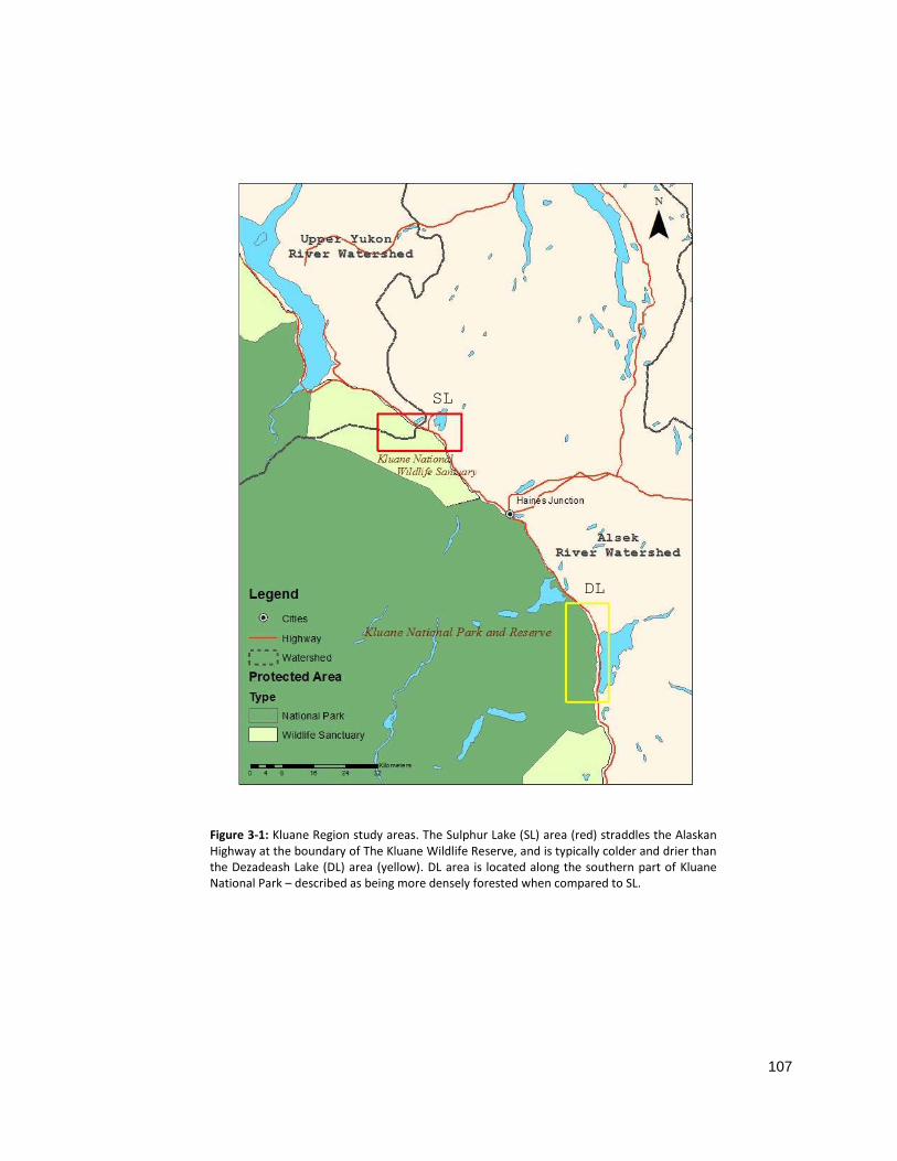
107
3.7 Figures and Tables
SL
DL
Figure 3-1: Kluane Region study areas. The Sulphur Lake (SL) area (red) straddles the Alaskan Highway at the boundary of The Kluane Wildlife Reserve, and is typically colder and drier than the Dezadeash Lake (DL) area (yellow). DL area is located along the southern part of Kluane National Park – described as being more densely forested when compared to SL.

108
Figure 3-2: Average monthly adjusted climate for Haines Junction from 1945 - 2010. Because remote sensing data is typically acquired in the summer, only climate data from the previous year was considered for months following August (final summer month). Bars represent mean precipitation per month; the dark line represents mean temperature. Total precipitation in Haines Junction is relatively low, the majority of which falls as snow. The Highest temperatures and total precipitation are experienced in July.
0
5
10
15
20
25
30
35
40
45
-25
-20
-15
-10
-5
0
5
10
15
S O N D J F M A M J J A
Me
an T
ota
l Pre
cip
itat
ion
(m
m)
Air
Te
mp
era
ture
(°C
)
Month
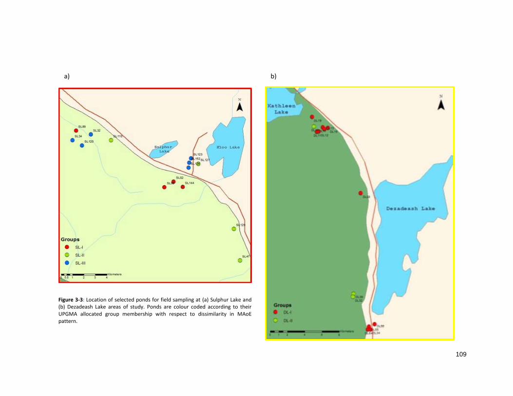
109
a) b)
Figure 3-3: Location of selected ponds for field sampling at (a) Sulphur Lake and (b) Dezadeash Lake areas of study. Ponds are colour coded according to their UPGMA allocated group membership with respect to dissimilarity in MAoE pattern.

110
1 10
Figure 3-4: A graphical representation of transect division by zone from shoreline to forest edge. Transects were extended from open water to forest edge as determined by abundance of trees or potential bathymetry. Each transect was divided into ten zones and numbered 1 (shoreline) to 10 (forest edge) indicating increasing distance from shoreline. The three largest live stems were sampled for each of the zones in addition to the largest dead stem. Number of dead stems sampled depended on the proportion of dead stems present at each pond. The oldest stem was considered the minimum age of establishment for that zone along a given transect. Minimum age of establishment per zone for a pond was defined by the median zone age of the three transects sampled.
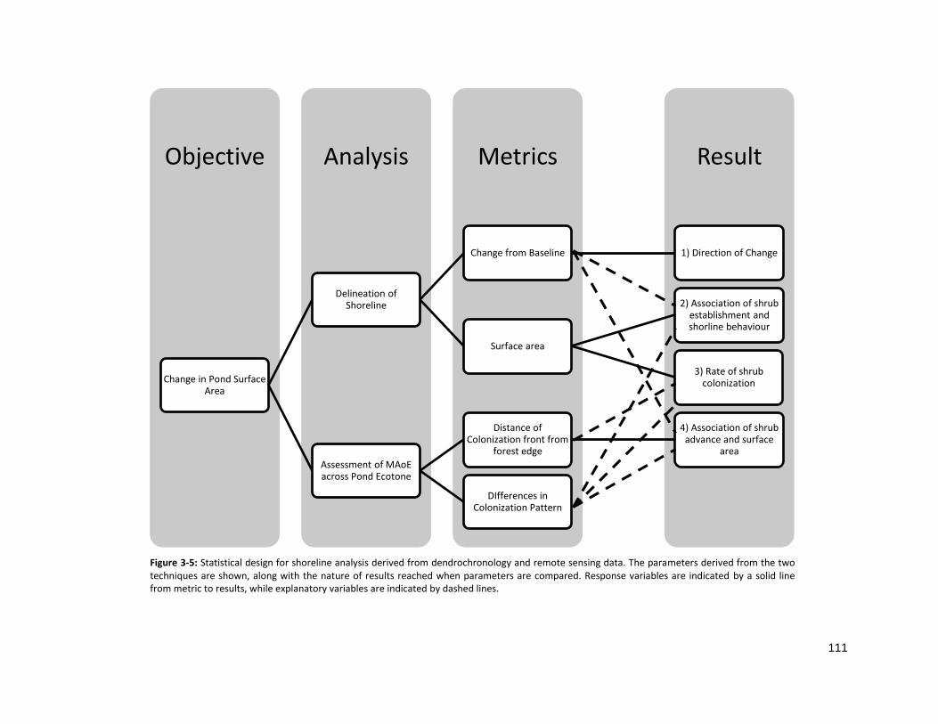
111
Result Metrics Analysis Objective
Change in Pond Surface Area
Delineation of Shoreline
Change from Baseline 1) Direction of Change
Surface area
2) Association of shrub establishment and shorline behaviour
3) Rate of shrub colonization
Assessment of MAoE across Pond Ecotone
Distance of Colonization front from
forest edge
4) Association of shrub advance and surface
area
DIfferences in Colonization Pattern
Figure 3-5: Statistical design for shoreline analysis derived from dendrochronology and remote sensing data. The parameters derived from the two techniques are shown, along with the nature of results reached when parameters are compared. Response variables are indicated by a solid line from metric to results, while explanatory variables are indicated by dashed lines.
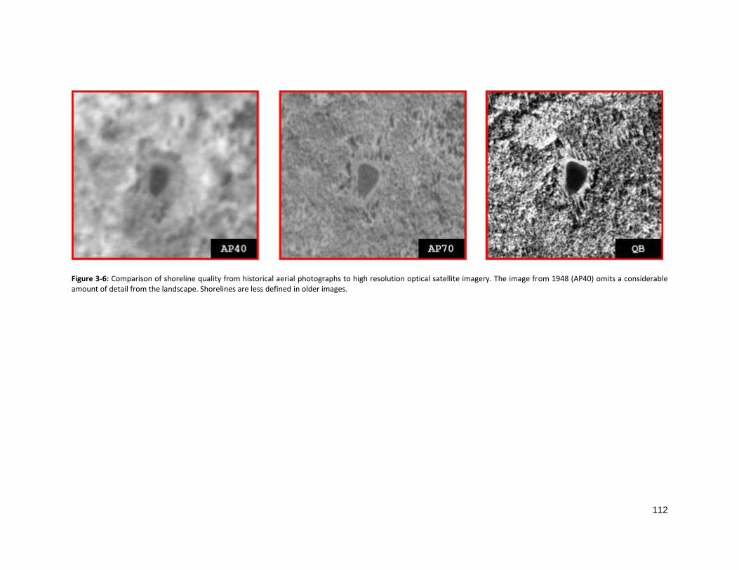
112
Figure 3-6: Comparison of shoreline quality from historical aerial photographs to high resolution optical satellite imagery. The image from 1948 (AP40) omits a considerable amount of detail from the landscape. Shorelines are less defined in older images.
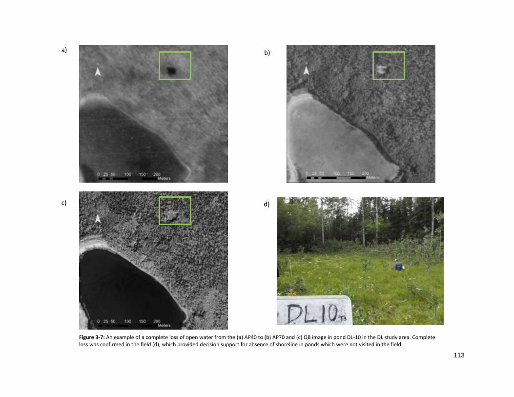
113
a) b)
c) d)
Figure 3-7: An example of a complete loss of open water from the (a) AP40 to (b) AP70 and (c) QB image in pond DL-10 in the DL study area. Complete loss was confirmed in the field (d), which provided decision support for absence of shoreline in ponds which were not visited in the field.
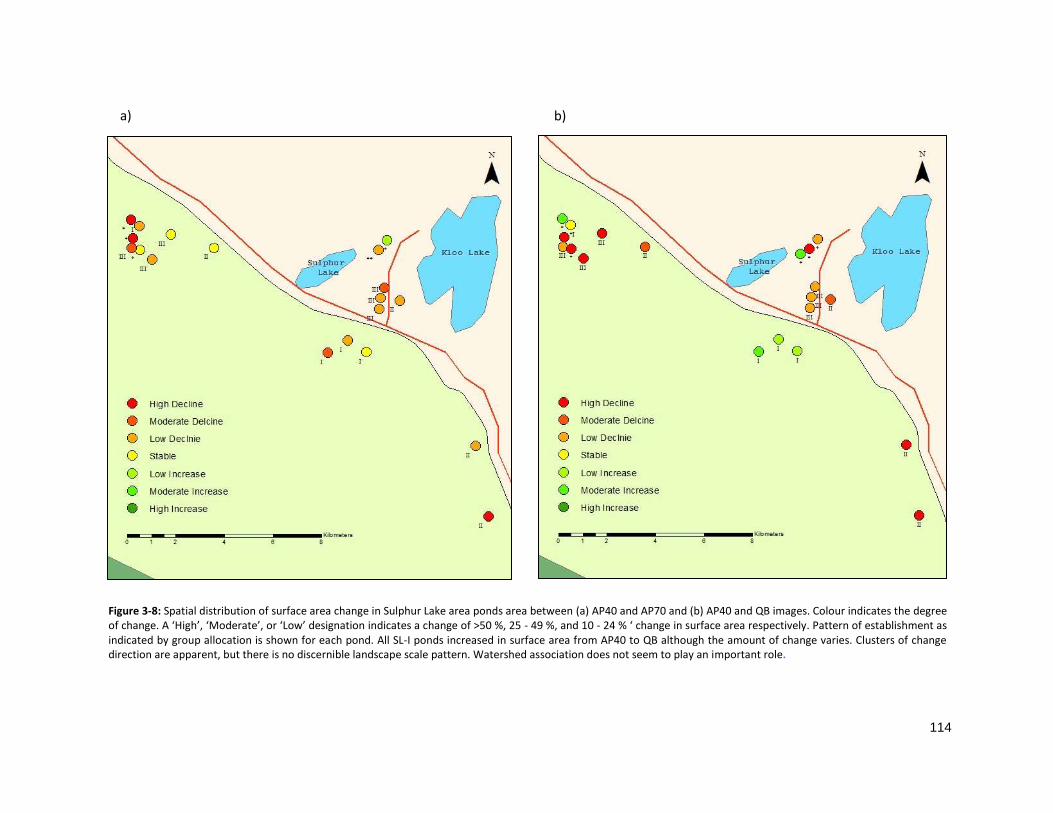
114
a) b)
Figure 3-8: Spatial distribution of surface area change in Sulphur Lake area ponds area between (a) AP40 and AP70 and (b) AP40 and QB images. Colour indicates the degree of change. A ‘High’, ‘Moderate’, or ‘Low’ designation indicates a change of >50 %, 25 - 49 %, and 10 - 24 % ‘ change in surface area respectively. Pattern of establishment as indicated by group allocation is shown for each pond. All SL-I ponds increased in surface area from AP40 to QB although the amount of change varies. Clusters of change direction are apparent, but there is no discernible landscape scale pattern. Watershed association does not seem to play an important role.
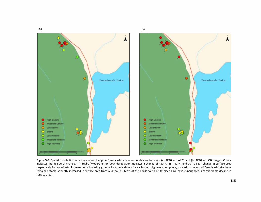
115
a) b)
Figure 3-9: Spatial distribution of surface area change in Dezadeash Lake area ponds area between (a) AP40 and AP70 and (b) AP40 and QB images. Colour indicates the degree of change. . A ‘High’, ‘Moderate’, or ‘Low’ designation indicates a change of >50 %, 25 - 49 %, and 10 - 24 % ‘ change in surface area respectively Pattern of establishment as indicated by group allocation is shown for each pond. High elevation ponds, located to the east of Dezadeash Lake, have remained stable or subtly increased in surface area from AP40 to QB. Most of the ponds south of Kathleen Lake have experienced a considerable decline in surface area.
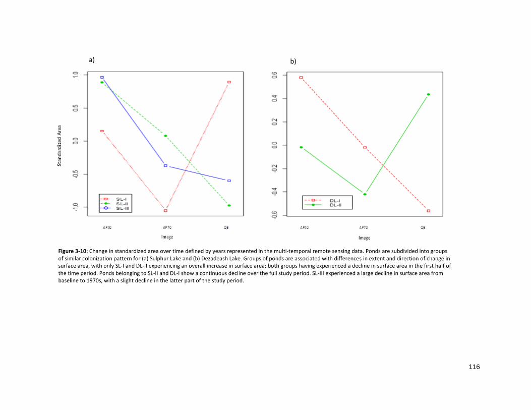
116
Figure 3-10: Change in standardized area over time defined by years represented in the multi-temporal remote sensing data. Ponds are subdivided into groups of similar colonization pattern for (a) Sulphur Lake and (b) Dezadeash Lake. Groups of ponds are associated with differences in extent and direction of change in surface area, with only SL-I and DL-II experiencing an overall increase in surface area; both groups having experienced a decline in surface area in the first half of the time period. Ponds belonging to SL-II and DL-I show a continuous decline over the full study period. SL-III experienced a large decline in surface area from baseline to 1970s, with a slight decline in the latter part of the study period.
a) b)
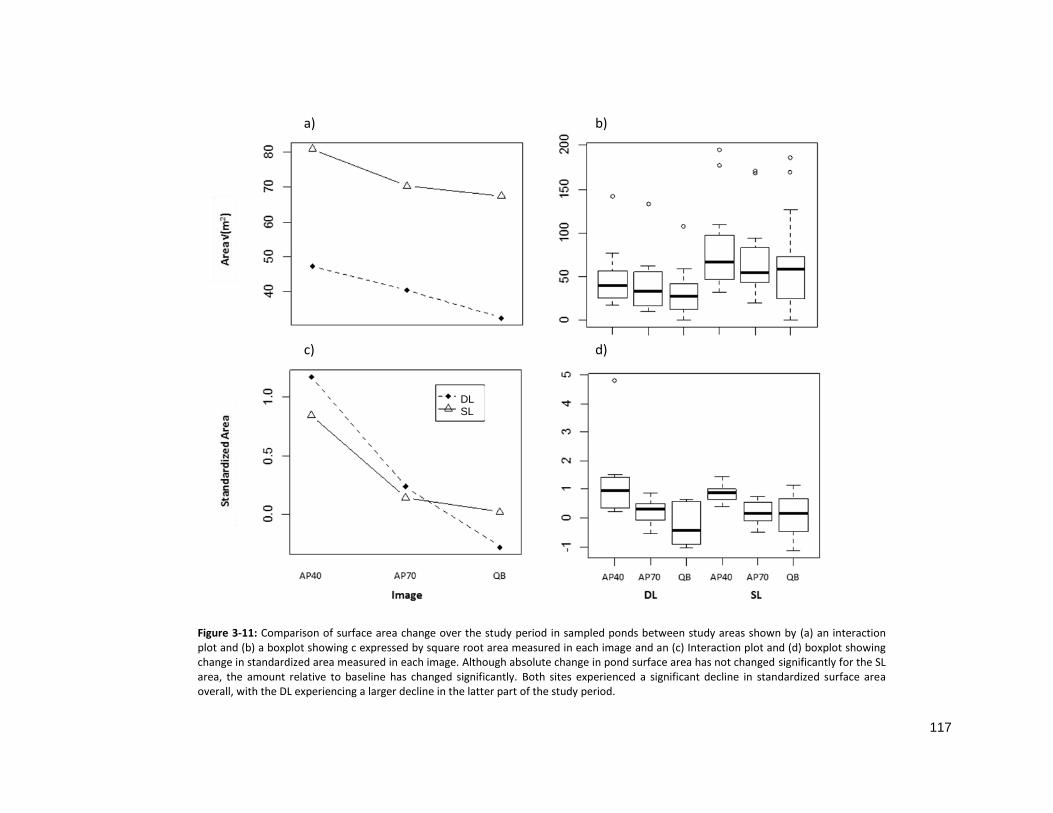
117
Figure 3-11: Comparison of surface area change over the study period in sampled ponds between study areas shown by (a) an interaction plot and (b) a boxplot showing c expressed by square root area measured in each image and an (c) Interaction plot and (d) boxplot showing change in standardized area measured in each image. Although absolute change in pond surface area has not changed significantly for the SL area, the amount relative to baseline has changed significantly. Both sites experienced a significant decline in standardized surface area overall, with the DL experiencing a larger decline in the latter part of the study period.
DL SL
a) b)
c) d)
118
Figure 3-12: Changes in shoreline position within the ecotone represented by advancement of shrub colonization front toward shoreline in each year of the remote sensing time series for the (a) SL and (b) DL study area, and (c) the Kluane Region. Colonization front is represented by furthest shrub establishment within the pond margin for the year represented by a remote sensing image, where 1 indicates shoreline and 11 indicates no encroachment into present day pond margin. Advancement of shrubs has increased significantly for both SL and DL areas; the rate of shrub advance into pond margins is similar for both study areas. Salix spp. had advanced much further into the ecotone by the 1970s in ponds belonging to SL-I than the other ponds in the SL area.
a) c) b)
119
Figure 3-13: Change in precipitation and mean air temperature, for the Kluane region, since 1945. Temperature has increased significantly by 0.04°C per year, for an average increase of 2.4°C, over the study period; with a notable increase in average temperature in the 1980s. Although much of the precipitation values are missing due to lack of station maintenance and data collection, precipitation does not show a similar trend for either Haines Junction or the City of Whitehorse
-500
-400
-300
-200
-100
0
100
200
300
400
500
-6.0
-4.0
-2.0
0.0
2.0
4.0
6.0
8.0
19
45
19
50
19
55
19
60
19
65
19
70
19
75
19
80
19
85
19
90
19
95
20
00
20
05
20
10
Me
an T
ota
l Pre
cip
itat
ion
(m
m)
Me
an A
ir T
em
pe
ratu
re (
°C)
Year
Haines Junction
Whitehorse
120
0
10
20
30
40
50
60
70
80
90
-25
-20
-15
-10
-5
0
5
10
15
20 Haines Junction
Whitehorse
-10
-5
0
5
10
-40
-30
-20
-10
0
10
20
30
40
Jan Feb Mar Apr May Jun Jul Aug Sep Oct Nov Dec
Month
-100
-80
-60
-40
-20
0
20
40
60
-12
-8
-4
0
4
8
12
16
S O N D J F M A M J J AMonth
Haines Junction 1977 Whitehorse 2011
-100
-80
-60
-40
-20
0
20
40
60
-8
-4
0
4
8
12
16
Me
an T
ota
l Pre
cip
itat
ion
(m
m)
Me
an A
ir T
em
pe
ratu
re (
ºC)
Haines Junction 1975 Whitehorse 2008
Haines Junction 2008
Figure 3-14: Climate values for years represented by remote sensing data. (a) Mean monthly climate values for 1948, the baseline image. Difference in climate from the baseline for years represented by AP70 and QB in (b) Sulphur Lake area and (c) Dezadeash Lake area. Climate data for 2011 is only available for the City of Whitehorse weather stations (c). Climate values for fall and winter are differences from the previous year. Temperatures in both AP70 and QB are higher in the spring at both study areas, reaching above freezing in April, one month earlier than 1948.
a)
b)
c)
121
Table 3-1: Image properties for aerial photographs acquired from the National Air Photo Library, Ottawa, Ontario, Canada
Area Roll Number Photo
Number Date Acquired
Original Scale
ASL (ft.) Pixel
Resolution (m)
Sulphur Lake A11447 297 7/5/1948 1:40000 20000 0.85 347 7/5/1948 1:40000 20000 0.85
A11478 161 7/5/1948 1:40000 20000 0.85 210 7/5/1948 1:40000 20000 0.85
A23792 4 7/8/1975 1:35000 17425 0.74 87 7/8/1975 1:35000 17425 0.74 130 7/8/1975 1:35000 17425 0.74
A23820 78 7/29/1974 1:35000 17000 0.74 Dezadeash
Lake A11452 211 6/25/1948 1:40000 20000 0.85
213 6/26/1948 1:40000 20000 0.85
216 6/27/1948 1:40000 20000 0.85
217 6/28/1948 1:40000 20000 0.85
218 6/29/1948 1:40000 20000 0.85
A24763 145 8/3/1977 1:80000 40000 1.69
146 8/4/1977 1:80000 40000 1.69
147 8/5/1977 1:80000 40000 1.69
148 8/6/1977 1:80000 40000 1.69
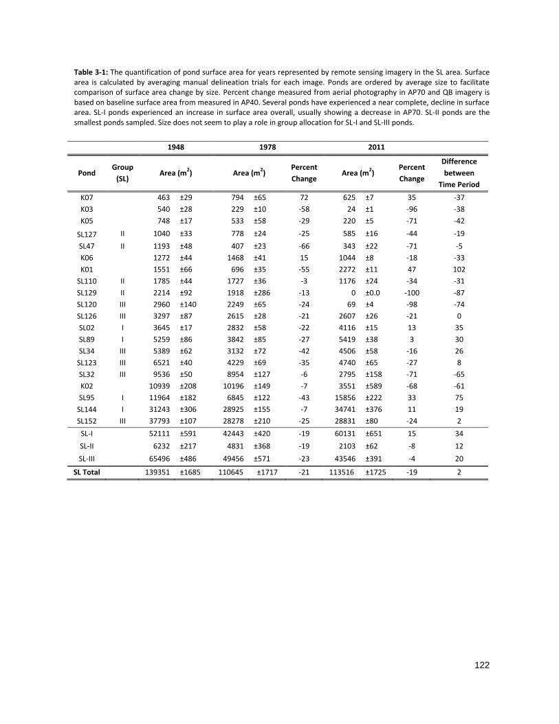
122
Table 3-1: The quantification of pond surface area for years represented by remote sensing imagery in the SL area. Surface area is calculated by averaging manual delineation trials for each image. Ponds are ordered by average size to facilitate comparison of surface area change by size. Percent change measured from aerial photography in AP70 and QB imagery is based on baseline surface area from measured in AP40. Several ponds have experienced a near complete, decline in surface area. SL-I ponds experienced an increase in surface area overall, usually showing a decrease in AP70. SL-II ponds are the smallest ponds sampled. Size does not seem to play a role in group allocation for SL-I and SL-III ponds.
1948 1978 2011
Pond Group
(SL) Area (m
2) Area (m
2)
Percent
Change Area (m
2)
Percent
Change
Difference
between
Time Period
K07 463 ±29 794 ±65 72 625 ±7 35 -37
K03 540 ±28 229 ±10 -58 24 ±1 -96 -38
K05 748 ±17 533 ±58 -29 220 ±5 -71 -42
SL127 II 1040 ±33 778 ±24 -25 585 ±16 -44 -19
SL47 II 1193 ±48 407 ±23 -66 343 ±22 -71 -5
K06 1272 ±44 1468 ±41 15 1044 ±8 -18 -33
K01 1551 ±66 696 ±35 -55 2272 ±11 47 102
SL110 II 1785 ±44 1727 ±36 -3 1176 ±24 -34 -31
SL129 II 2214 ±92 1918 ±286 -13 0 ±0.0 -100 -87
SL120 III 2960 ±140 2249 ±65 -24 69 ±4 -98 -74
SL126 III 3297 ±87 2615 ±28 -21 2607 ±26 -21 0
SL02 I 3645 ±17 2832 ±58 -22 4116 ±15 13 35
SL89 I 5259 ±86 3842 ±85 -27 5419 ±38 3 30
SL34 III 5389 ±62 3132 ±72 -42 4506 ±58 -16 26
SL123 III 6521 ±40 4229 ±69 -35 4740 ±65 -27 8
SL32 III 9536 ±50 8954 ±127 -6 2795 ±158 -71 -65
K02 10939 ±208 10196 ±149 -7 3551 ±589 -68 -61
SL95 I 11964 ±182 6845 ±122 -43 15856 ±222 33 75
SL144 I 31243 ±306 28925 ±155 -7 34741 ±376 11 19
SL152 III 37793 ±107 28278 ±210 -25 28831 ±80 -24 2
SL-I 52111 ±591 42443 ±420 -19 60131 ±651 15 34
SL-II 6232 ±217 4831 ±368 -19 2103 ±62 -8 12
SL-III 65496 ±486 49456 ±571 -23 43546 ±391 -4 20
SL Total 139351 ±1685 110645 ±1717 -21 113516 ±1725 -19 2
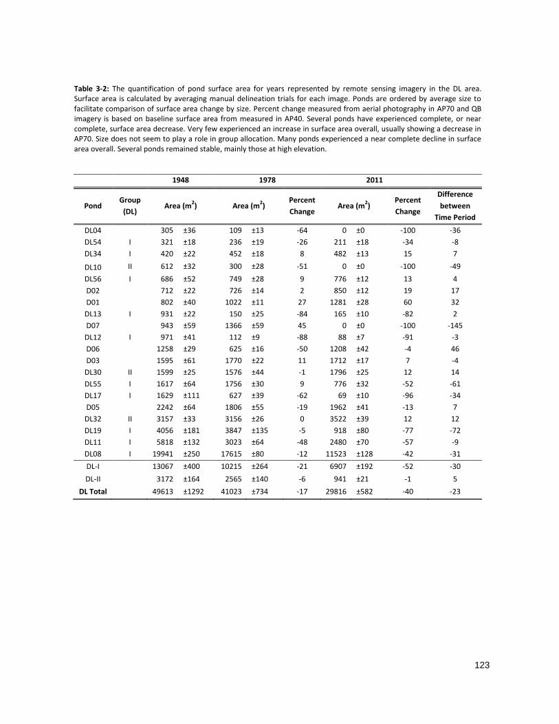
123
Table 3-2: The quantification of pond surface area for years represented by remote sensing imagery in the DL area. Surface area is calculated by averaging manual delineation trials for each image. Ponds are ordered by average size to facilitate comparison of surface area change by size. Percent change measured from aerial photography in AP70 and QB imagery is based on baseline surface area from measured in AP40. Several ponds have experienced complete, or near complete, surface area decrease. Very few experienced an increase in surface area overall, usually showing a decrease in AP70. Size does not seem to play a role in group allocation. Many ponds experienced a near complete decline in surface area overall. Several ponds remained stable, mainly those at high elevation.
1948 1978 2011
Pond Group
(DL) Area (m
2) Area (m
2)
Percent
Change Area (m
2)
Percent
Change
Difference
between
Time Period
DL04 305 ±36 109 ±13 -64 0 ±0 -100 -36
DL54 I 321 ±18 236 ±19 -26 211 ±18 -34 -8
DL34 I 420 ±22 452 ±18 8 482 ±13 15 7
DL10 II 612 ±32 300 ±28 -51 0 ±0 -100 -49
DL56 I 686 ±52 749 ±28 9 776 ±12 13 4
D02 712 ±22 726 ±14 2 850 ±12 19 17
D01 802 ±40 1022 ±11 27 1281 ±28 60 32
DL13 I 931 ±22 150 ±25 -84 165 ±10 -82 2
D07 943 ±59 1366 ±59 45 0 ±0 -100 -145
DL12 I 971 ±41 112 ±9 -88 88 ±7 -91 -3
D06 1258 ±29 625 ±16 -50 1208 ±42 -4 46
D03 1595 ±61 1770 ±22 11 1712 ±17 7 -4
DL30 II 1599 ±25 1576 ±44 -1 1796 ±25 12 14
DL55 I 1617 ±64 1756 ±30 9 776 ±32 -52 -61
DL17 I 1629 ±111 627 ±39 -62 69 ±10 -96 -34
D05 2242 ±64 1806 ±55 -19 1962 ±41 -13 7
DL32 II 3157 ±33 3156 ±26 0 3522 ±39 12 12
DL19 I 4056 ±181 3847 ±135 -5 918 ±80 -77 -72
DL11 I 5818 ±132 3023 ±64 -48 2480 ±70 -57 -9
DL08 I 19941 ±250 17615 ±80 -12 11523 ±128 -42 -31
DL-I 13067 ±400 10215 ±264 -21 6907 ±192 -52 -30
DL-II 3172 ±164 2565 ±140 -6 941 ±21 -1 5
DL Total 49613 ±1292 41023 ±734 -17 29816 ±582 -40 -23
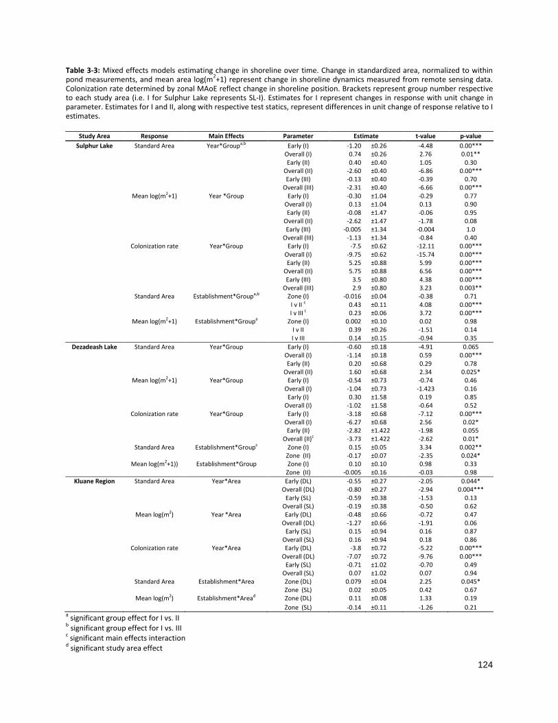
124
Table 3-3: Mixed effects models estimating change in shoreline over time. Change in standardized area, normalized to within pond measurements, and mean area log(m
2+1) represent change in shoreline dynamics measured from remote sensing data.
Colonization rate determined by zonal MAoE reflect change in shoreline position. Brackets represent group number respective to each study area (i.e. I for Sulphur Lake represents SL-I). Estimates for I represent changes in response with unit change in parameter. Estimates for I and II, along with respective test statics, represent differences in unit change of response relative to I estimates.
a significant group effect for I vs. II
b significant group effect for I vs. III
c significant main effects interaction
d significant study area effect
Study Area Response Main Effects Parameter Estimate t-value p-value
Sulphur Lake Standard Area Year*Groupa,b Early (I) -1.20 ±0.26 -4.48 0.00*** Overall (I) 0.74 ±0.26 2.76 0.01** Early (II) 0.40 ±0.40 1.05 0.30 Overall (II) -2.60 ±0.40 -6.86 0.00*** Early (III) -0.13 ±0.40 -0.39 0.70 Overall (III) -2.31 ±0.40 -6.66 0.00*** Mean log(m2+1) Year *Group Early (I) -0.30 ±1.04 -0.29 0.77 Overall (I) 0.13 ±1.04 0.13 0.90 Early (II) -0.08 ±1.47 -0.06 0.95 Overall (II) -2.62 ±1.47 -1.78 0.08 Early (III) -0.005 ±1.34 -0.004 1.0 Overall (III) -1.13 ±1.34 -0.84 0.40 Colonization rate Year*Group Early (I) -7.5 ±0.62 -12.11 0.00*** Overall (I) -9.75 ±0.62 -15.74 0.00*** Early (II) 5.25 ±0.88 5.99 0.00*** Overall (II) 5.75 ±0.88 6.56 0.00*** Early (III) 3.5 ±0.80 4.38 0.00*** Overall (III) 2.9 ±0.80 3.23 0.003** Standard Area Establishment*Groupa,b Zone (I) -0.016 ±0.04 -0.38 0.71 I v II c 0.43 ±0.11 4.08 0.00*** I v III c 0.23 ±0.06 3.72 0.00*** Mean log(m2+1) Establishment*Groupa Zone (I) 0.002 ±0.10 0.02 0.98 I v II 0.39 ±0.26 -1.51 0.14 I v III 0.14 ±0.15 -0.94 0.35
Dezadeash Lake Standard Area Year*Group Early (I) -0.60 ±0.18 -4.91 0.065 Overall (I) -1.14 ±0.18 0.59 0.00*** Early (II) 0.20 ±0.68 0.29 0.78 Overall (II) 1.60 ±0.68 2.34 0.025* Mean log(m2+1) Year*Group Early (I) -0.54 ±0.73 -0.74 0.46 Overall (I) -1.04 ±0.73 -1.423 0.16 Early (I) 0.30 ±1.58 0.19 0.85 Overall (I) -1.02 ±1.58 -0.64 0.52 Colonization rate Year*Group Early (I) -3.18 ±0.68 -7.12 0.00*** Overall (I) -6.27 ±0.68 2.56 0.02* Early (II) -2.82 ±1.422 -1.98 0.055 Overall (II)c -3.73 ±1.422 -2.62 0.01* Standard Area Establishment*Groupc Zone (I) 0.15 ±0.05 3.34 0.002** Zone (II) -0.17 ±0.07 -2.35 0.024* Mean log(m2+1)) Establishment*Group Zone (I) 0.10 ±0.10 0.98 0.33 Zone (II) -0.005 ±0.16 -0.03 0.98
Kluane Region Standard Area Year*Area Early (DL) -0.55 ±0.27 -2.05 0.044* Overall (DL) -0.80 ±0.27 -2.94 0.004*** Early (SL) -0.59 ±0.38 -1.53 0.13 Overall (SL) -0.19 ±0.38 -0.50 0.62 Mean log(m2) Year *Area Early (DL) -0.48 ±0.66 -0.72 0.47 Overall (DL) -1.27 ±0.66 -1.91 0.06 Early (SL) 0.15 ±0.94 0.16 0.87 Overall (SL) 0.16 ±0.94 0.18 0.86 Colonization rate Year*Area Early (DL) -3.8 ±0.72 -5.22 0.00*** Overall (DL) -7.07 ±0.72 -9.76 0.00*** Early (SL) -0.71 ±1.02 -0.70 0.49 Overall (SL) 0.07 ±1.02 0.07 0.94 Standard Area Establishment*Area Zone (DL) 0.079 ±0.04 2.25 0.045* Zone (SL) 0.02 ±0.05 0.42 0.67 Mean log(m2) Establishment*Aread Zone (DL) 0.11 ±0.08 1.33 0.19
Zone (SL) -0.14 ±0.11 -1.26 0.21
125
CHAPTER 4: CONCLUSIONS
Change detection in inland water surface area is usually based on temporally limited remote sensing
data, limiting the ability to make conclusions about long-term trends. The research presented in this
thesis demonstrates the value of shrub-based dendrochronology for describing recent changes in
shoreline behaviour in small ponds. The predictable annual growth of woody vegetation provides an
opportunity to supplement the lack of direct observation in Arctic systems with natural high resolution
chronosequences measured from vegetation. On their own, the shrub dendrochronology and remote
sensing time series were unable to provide a complete picture of shoreline behaviour in the southwest
Yukon. While shoreline position reported in remote sensing time series indicates a rise in water level for
a few ponds in both study areas, the dendrochronological data suggests different hydrological regimes
are experienced by each. Nondecreasing ponds in the Sulphur Lake area exhibit a highly dynamic
shoreline as shown by the high mortality of mature shrubs in the nearshore, while high elevation ponds
in the Dezadeash Lake area maintain a more stable shoreline indicated by the relatively high abundance
of live, mature stems. In addition, combined with the characteristic population evidence, colonization
rates and population structure suggest a long-term trend toward shoreline recession for nondecreasing
ponds in the Sulphur Lake area. Although the mechanism could not adequately be determined, the
study highlights the issues related to investigating primary driving mechanism based on incomplete
historical data and lack of direct measurement.
Small ponds in the Kluane region have experienced an overall decline in surface area since 1948. In
this study, availability of seasonally consistent time periods was limited to three images, which were
supplemented with a proxy of shoreline behaviour inferred from dendrochronology. Variability in
shoreline behaviour across the landscape was reflected in homogenous patterns of establishment within
pond ecotones. In addition, the timing of major surface area losses in the decreasing ponds

126
corresponded with the rate of ecotone colonization by tall shrubs. The majority of ponds experienced a
gradual advance of colonization front towards the shoreline, while some ponds exhibited more of a
dynamic or stable shoreline, with periods of decline followed by periods of high water level.
The overall trend in surface area change measured through remote sensing shows general decline in
surface area for ponds sampled in the Kluane Region. This trend is supported by the trend in shrub
colonization toward shoreline, suggesting recent and directional transition of pond ecotones to
terrestrial shrub ecosystems. Evidence for the reliability of shrub dynamics in characterizing shoreline
dynamics is supported by the association of zonal shrub establishment with differences in population
structure and ecotone colonization rates. Identical establishment patterns were obtained when
population variables were used to predict colonization rates, reflecting the hydrological regimes
associated with similar ponds. These parallel relationships are highly valuable for regions where
historical imagery is unavailable, an issue that is common throughout the Arctic.
The number of small lakes in the North (>0.05 km2) far outnumber the incidence of large lakes which
are typically the focus of change detection in Arctic lake surface area. Although indirectly suggested
from the relation between colonization rates, pattern of establishment of similar ponds, and change in
water surface area measured from remotely sensed imagery, more attention needs to be given to the
natural variability of small ponds in the Arctic; particularly in the face of a changing climate. These small
lakes are more prone to change due to their shallow depth. The vegetation dynamics and variability in
shoreline behaviour suggest that hydrological regimes are spatially heterogeneous; not only within
study regions but also across climatic gradients. Because these regimes are currently unknown, future
research must integrate long term monitoring of pond water levels with broader scale temporal data. In
addition, the mechanism of advance, effects of pond and ecotone population structure, and rate of
ecesis are also unknown, making a lagged response hard to quantify without direct observational data. A
characterization of the hydrology of small ponds, as well as an understanding the physiological

127
responses of dendrochronologically valuable shrub species, is crucial to developing comprehensive
trends in surface hydrology.
This study has also highlighted the importance of cross-dating ring-widths in shrub population
studies utilizing principles of dendrochronology. Although shrub dendrochronology relies on the
acceptance of certain limitations and assumptions, the results illustrate the consequences of omitting
dead samples from the chronosequencing of vegetation dynamics. More dynamic shorelines were
completely overlooked when dead individuals were excluded, and MAoE in the nearshore was
misrepresented which resulted in erroneous and misleading conclusions ecotone dynamics in SL ponds.
Developing accurate chronologies of shoreline behaviour can only be accomplished with the inclusion of
all establishment data, regardless of shrub mortality.
Gradual colonization and correspondence with warming temperatures suggest that the drying of
pond margins is the most likely cause of decreasing pond extent. This response may be due to longer
growing seasons and extended ice free periods, associated with higher levels of potential
evapotranspiration, exacerbated by stable precipitation in the region. The combination of sporadic
permafrost throughout the region of study, and the similarity in pond characteristics suggest that spatial
heterogeneity in hydrological regimes and water balance may cause a rise in water level in non-
decreasing ponds. Wetlands are critical habitat for a number of northern aquatic species. A negative
imbalance in precipitation-evaporation ratios, combined with increased transpiration from colonization
of tall shrubs in the pond-margin ecotone may accelerate pond recession in the Kluane Region, with
significant ecological consequences. The successful implementation of these techniques has value for
areas that are most sensitive to climate change and lack direct, long-term measurement of
environmental conditions. From a conservation perspective, this analysis provides an enhanced ability to
predict likely consequences of changing disturbance regimes and ecosystem response in northern
landscapes.
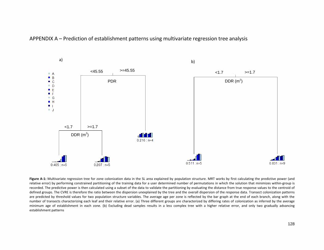
128
APPENDIX A – Prediction of establishment patterns using multivariate regression tree analysis
Figure A-1: Multivariate regression tree for zone colonization data in the SL area explained by population structure. MRT works by first calculating the predictive power (and relative error) by performing constrained partitioning of the training data for a user determined number of permutations in which the solution that minimizes within-group is recorded. The predictive power is then calculated using a subset of the data to validate the partitioning by evaluating the distance from true response values to the centroid of defined groups. The CVRE is therefore the ratio between the dispersion unexplained by the tree and the overall dispersion of the response data. Transect colonization patterns are predicted by threshold values for two population structure variables. The average age per zone is reflected by the bar graph at the end of each branch, along with the number of transects characterizing each leaf and their relative error. (a) Three different groups are characterized by differing rates of colonization as inferred by the average minimum age of establishment in each zone. (b) Excluding dead samples results in a less complex tree with a higher relative error, and only two gradually advancing establishment patterns
PDR
>=45.55 <45.55
DDR (m2)
DDR (m2)
>=1.7 <1.7
>=1.7 <1.7
a) b)

129
Figure A-2: Multivariate regression tree for zone colonization data in the DL area explained by population structure. MRT works by first calculating the predictive power (and relative error) by performing constrained partitioning of the training data for a user determined number of permutations in which the solution that minimizes within-group is recorded. The predictive power is then calculated using a subset of the data to validate the partitioning by evaluating the distance from true response values to the centroid of defined groups. The CVRE is therefore the ratio between the dispersion unexplained by the tree and the overall dispersion of the response data. Transect colonization patterns are predicted by threshold values for two population structure variables. Two different groups are characterized by differing rates of colonization as inferred by the average minimum age of establishment in each zone. Only variable was relevant in determining allocation of transects to groups, with very few allocated to that representing a more stable colonization pattern.
DLR (m2)
>=7.1 <7.1
DLS (m2)
>=2.65 <2.65
a) b)
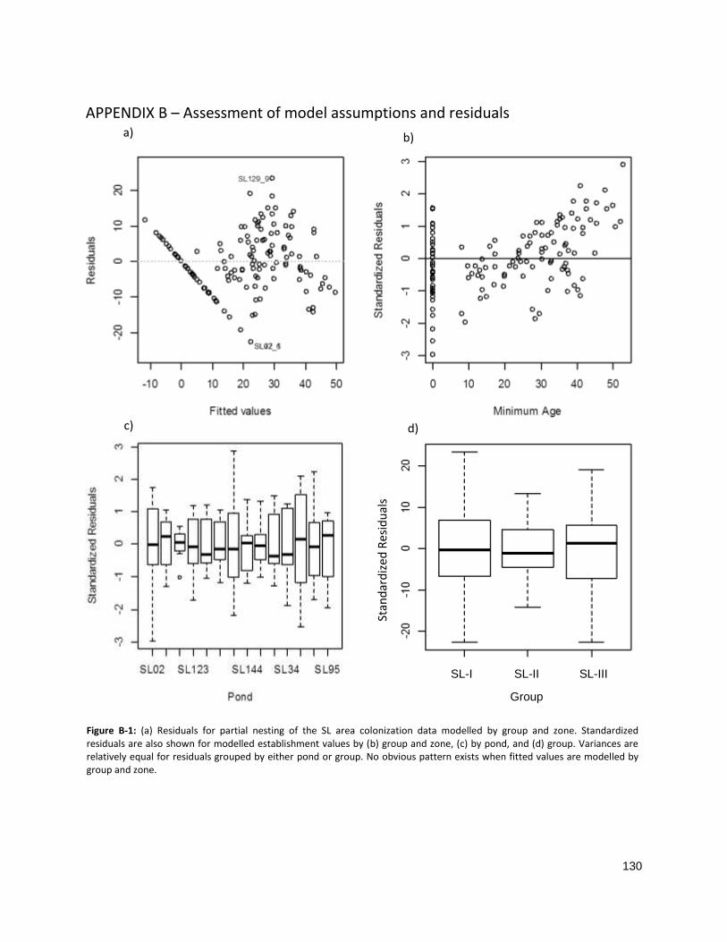
130
SL-I SL-II SL-III
Group
APPENDIX B – Assessment of model assumptions and residuals
c) d)
Stan
dar
diz
ed R
esi
du
als
b) a)
Figure B-1: (a) Residuals for partial nesting of the SL area colonization data modelled by group and zone. Standardized residuals are also shown for modelled establishment values by (b) group and zone, (c) by pond, and (d) group. Variances are relatively equal for residuals grouped by either pond or group. No obvious pattern exists when fitted values are modelled by group and zone.
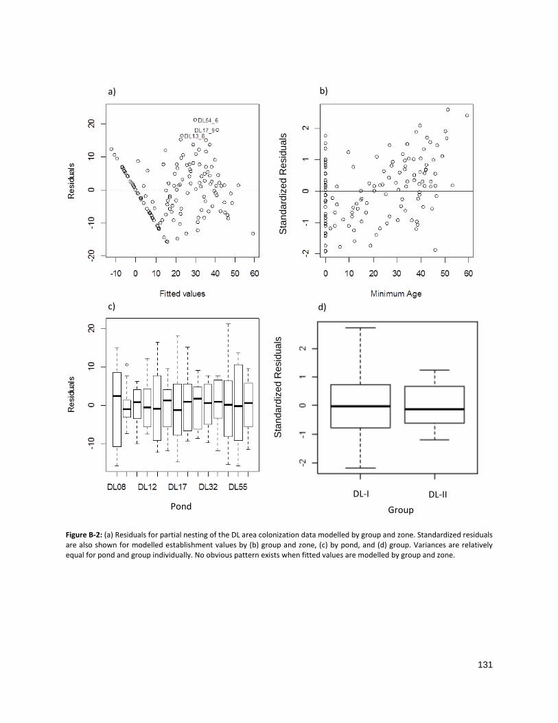
131
Figure B-2: (a) Residuals for partial nesting of the DL area colonization data modelled by group and zone. Standardized residuals are also shown for modelled establishment values by (b) group and zone, (c) by pond, and (d) group. Variances are relatively equal for pond and group individually. No obvious pattern exists when fitted values are modelled by group and zone.
Sta
nda
rdiz
ed
Re
sid
uals
S
tan
da
rdiz
ed
Re
sid
uals
DL-I DL-II
Group Pond
a) b)
c) d)
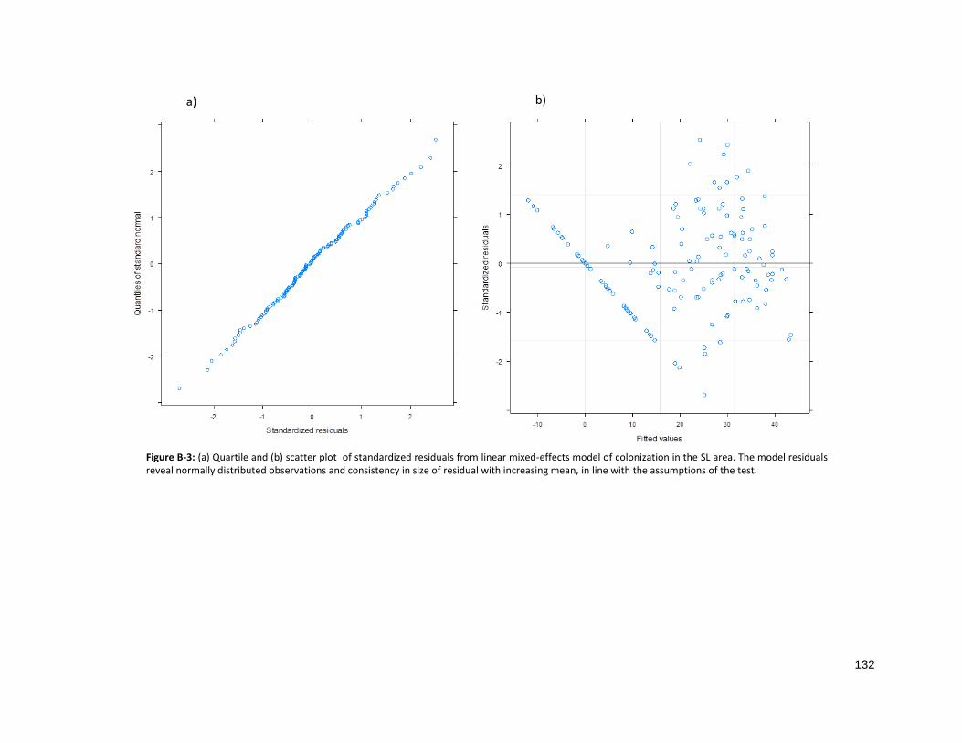
132
a) b)
Figure B-3: (a) Quartile and (b) scatter plot of standardized residuals from linear mixed-effects model of colonization in the SL area. The model residuals reveal normally distributed observations and consistency in size of residual with increasing mean, in line with the assumptions of the test.
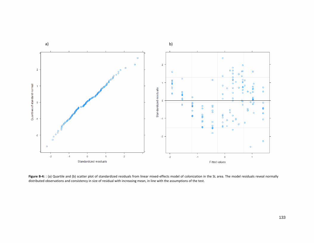
133
Figure B-4: : (a) Quartile and (b) scatter plot of standardized residuals from linear mixed-effects model of colonization in the SL area. The model residuals reveal normally
distributed observations and consistency in size of residual with increasing mean, in line with the assumptions of the test.
b) a)
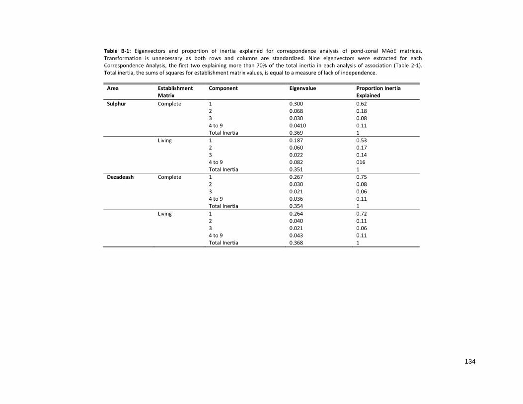
134
Table B-1: Eigenvectors and proportion of inertia explained for correspondence analysis of pond-zonal MAoE matrices. Transformation is unnecessary as both rows and columns are standardized. Nine eigenvectors were extracted for each Correspondence Analysis, the first two explaining more than 70% of the total inertia in each analysis of association (Table 2-1). Total inertia, the sums of squares for establishment matrix values, is equal to a measure of lack of independence.
Area Establishment Matrix
Component Eigenvalue Proportion Inertia Explained
Sulphur Complete 1 0.300 0.62 2 0.068 0.18 3 0.030 0.08 4 to 9 0.0410 0.11 Total Inertia 0.369 1
Living 1 0.187 0.53 2 0.060 0.17 3 0.022 0.14 4 to 9 0.082 016 Total Inertia 0.351 1
Dezadeash Complete 1 0.267 0.75 2 0.030 0.08 3 0.021 0.06 4 to 9 0.036 0.11 Total Inertia 0.354 1
Living 1 0.264 0.72 2 0.040 0.11 3 0.021 0.06 4 to 9 0.043 0.11 Total Inertia 0.368 1
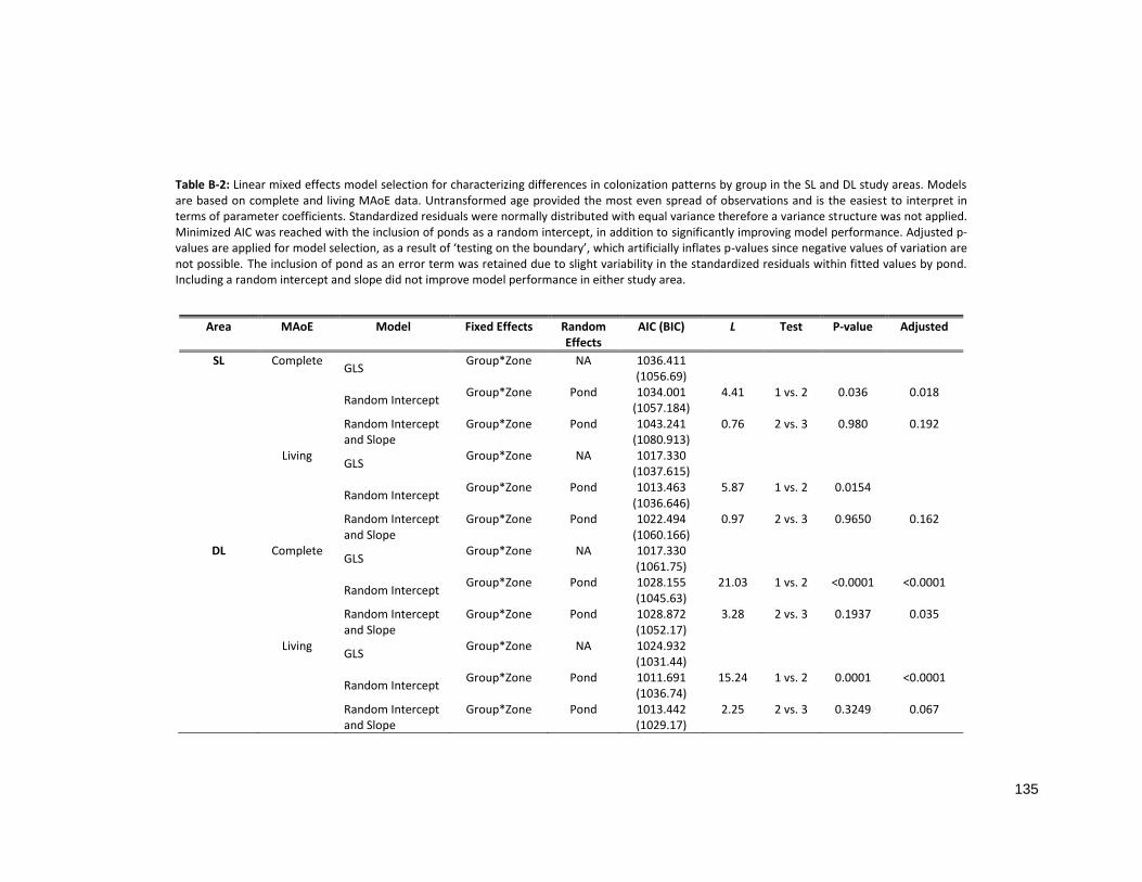
135
Table B-2: Linear mixed effects model selection for characterizing differences in colonization patterns by group in the SL and DL study areas. Models are based on complete and living MAoE data. Untransformed age provided the most even spread of observations and is the easiest to interpret in terms of parameter coefficients. Standardized residuals were normally distributed with equal variance therefore a variance structure was not applied. Minimized AIC was reached with the inclusion of ponds as a random intercept, in addition to significantly improving model performance. Adjusted p-values are applied for model selection, as a result of ‘testing on the boundary’, which artificially inflates p-values since negative values of variation are not possible. The inclusion of pond as an error term was retained due to slight variability in the standardized residuals within fitted values by pond. Including a random intercept and slope did not improve model performance in either study area.
Area MAoE Model Fixed Effects Random Effects
AIC (BIC) L Test P-value Adjusted
SL Complete GLS
Group*Zone NA 1036.411 (1056.69)
Random Intercept
Group*Zone Pond 1034.001 (1057.184)
4.41 1 vs. 2 0.036 0.018
Random Intercept and Slope
Group*Zone Pond 1043.241 (1080.913)
0.76 2 vs. 3 0.980 0.192
Living GLS
Group*Zone NA 1017.330 (1037.615)
Random Intercept
Group*Zone Pond 1013.463 (1036.646)
5.87
1 vs. 2 0.0154
Random Intercept and Slope
Group*Zone Pond 1022.494 (1060.166)
0.97 2 vs. 3 0.9650 0.162
DL Complete GLS
Group*Zone NA 1017.330 (1061.75)
Random Intercept
Group*Zone Pond 1028.155 (1045.63)
21.03 1 vs. 2 <0.0001
<0.0001
Random Intercept and Slope
Group*Zone Pond 1028.872 (1052.17)
3.28
2 vs. 3 0.1937
0.035
Living GLS
Group*Zone NA 1024.932 (1031.44)
Random Intercept
Group*Zone Pond 1011.691 (1036.74)
15.24 1 vs. 2 0.0001 <0.0001
Random Intercept and Slope
Group*Zone Pond 1013.442 (1029.17)
2.25 2 vs. 3 0.3249 0.067

136
APPENDIX C – GCP selection and image registration Uniform topography was considered important for feature geometry and accuracy in pixel
registration. Because of the highly heterogeneous terrain, GCPs were restricted to low lying areas with
even topography which is a reasonable compromise as the features of interest were found only in this
area. While it has been suggested that GCPs be spaced evenly over the image to be rectified, according
to Hughes et al. (2006) this practice may unnecessarily skew transformations to topographically complex
areas in historical aerial photographs. This is especially true in mountain regions such as in the Kluane
National Park, where the ‘greenbelt’ is directly adjacent to the high relief one of the most extensive
mountain ranges in North America where GCPs would be far removed, vertically, from the ponds. Better
accuracy may therefore be obtained by concentrating GCPs near the features of interest (Hughes et al.,
2006), in this case the ponds. The lack of static or man-made features in the region meant that only soft
classifiers – feature with fuzzy edges – were available; potentially effecting the overall registration error.
Solitary trees and rock outcrops fit the criteria better than any other feature, and where almost
exclusively used for GCPs. Discerning trees in the panchromatic aerial photograph images from
surrounding landscape proved to be a challenge. Sun angle was determined from the direction of
shadow, the base of which was taken as the top of the tree.
Accuracy is critical in change detection analysis, and challenging given the low quality of historical
images. Therefore, for each area of interest, at least one Ground Control Point (GCP) was established for
every square kilometer of the area containing sampled ponds. A second order polynomial fit was
employed due to the variability in terrain (Hughes et al., 2006) and images were rectified only when the
RMSE for pixel resolution was equivalent to no more than 0.6m on the ground. Higher order
polynomials produce coefficients that more closely models geometric disparity in the APs. Although this
improves accuracy in areas surrounding GCPs while potentially producing errors at greater distances
(Jensen, 2007), the majority of GCPs fell within close proximity to ponds under study. A cubic

137
convolution resampling method was applied to the panchromatic aerial photographs prior to manual
delineation; which assigns a reference location based on weighted values of the 16 pixels surrounding
the pixel being registered. This technique creates smoothed boundaries at the pond margin which
facilitates manual digitization of natural boundaries (Hughes et al., 2006; Sannel and Brown, 2010) (Fig
C-1). The disadvantage of cubic convolution resampling is the resulting distortion of the original spectral
data; which was not an issue when using only the panchromatic images and avoiding delineation
techniques which involve pixel classification.
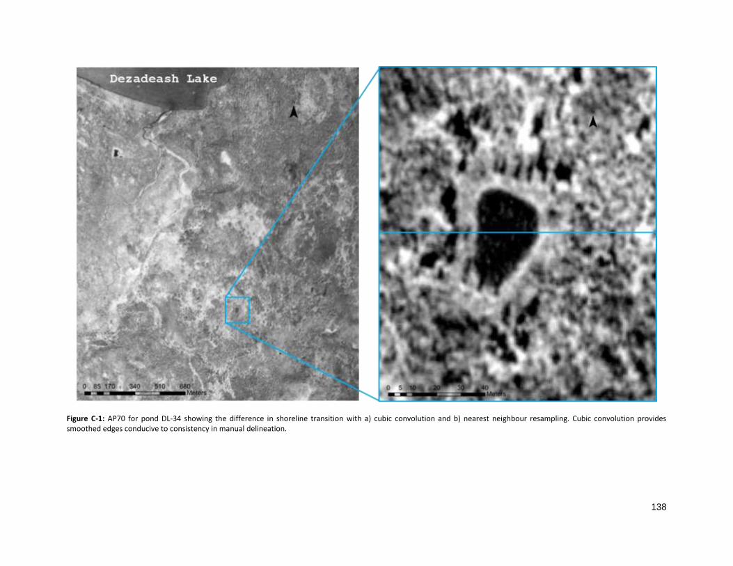
138
Figure C-1: AP70 for pond DL-34 showing the difference in shoreline transition with a) cubic convolution and b) nearest neighbour resampling. Cubic convolution provides smoothed edges conducive to consistency in manual delineation.
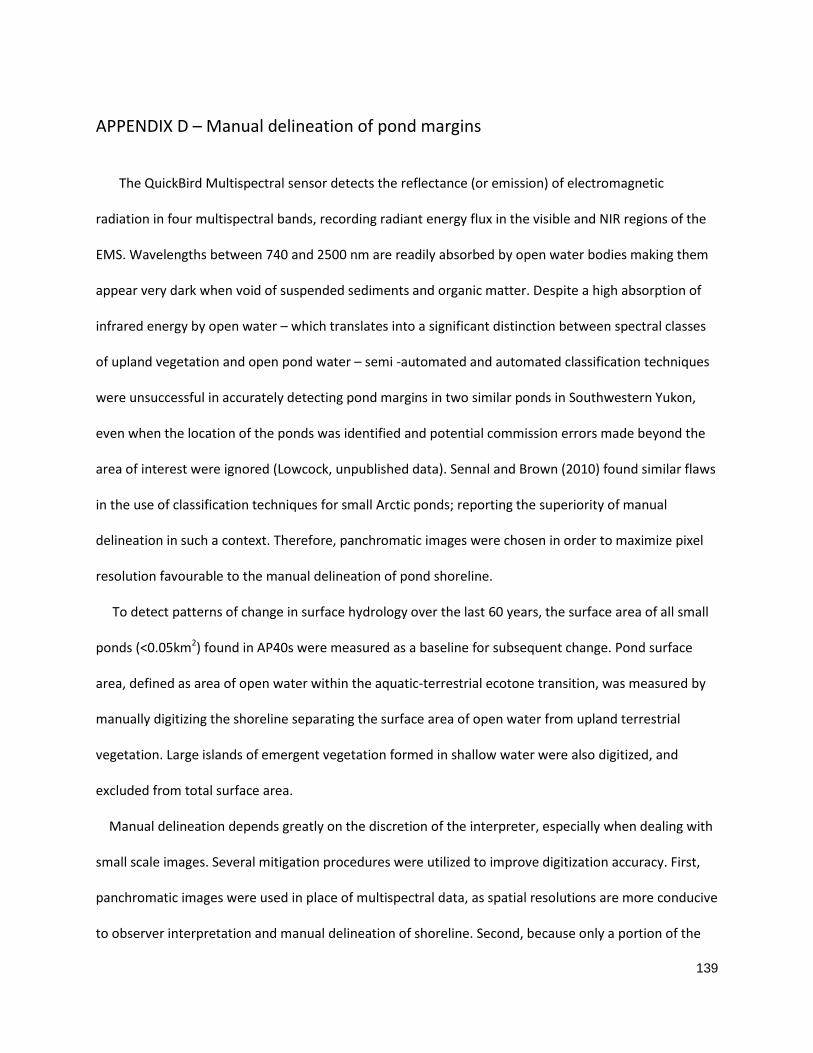
139
APPENDIX D – Manual delineation of pond margins
The QuickBird Multispectral sensor detects the reflectance (or emission) of electromagnetic
radiation in four multispectral bands, recording radiant energy flux in the visible and NIR regions of the
EMS. Wavelengths between 740 and 2500 nm are readily absorbed by open water bodies making them
appear very dark when void of suspended sediments and organic matter. Despite a high absorption of
infrared energy by open water – which translates into a significant distinction between spectral classes
of upland vegetation and open pond water – semi -automated and automated classification techniques
were unsuccessful in accurately detecting pond margins in two similar ponds in Southwestern Yukon,
even when the location of the ponds was identified and potential commission errors made beyond the
area of interest were ignored (Lowcock, unpublished data). Sennal and Brown (2010) found similar flaws
in the use of classification techniques for small Arctic ponds; reporting the superiority of manual
delineation in such a context. Therefore, panchromatic images were chosen in order to maximize pixel
resolution favourable to the manual delineation of pond shoreline.
To detect patterns of change in surface hydrology over the last 60 years, the surface area of all small
ponds (<0.05km2) found in AP40s were measured as a baseline for subsequent change. Pond surface
area, defined as area of open water within the aquatic-terrestrial ecotone transition, was measured by
manually digitizing the shoreline separating the surface area of open water from upland terrestrial
vegetation. Large islands of emergent vegetation formed in shallow water were also digitized, and
excluded from total surface area.
Manual delineation depends greatly on the discretion of the interpreter, especially when dealing with
small scale images. Several mitigation procedures were utilized to improve digitization accuracy. First,
panchromatic images were used in place of multispectral data, as spatial resolutions are more conducive
to observer interpretation and manual delineation of shoreline. Second, because only a portion of the
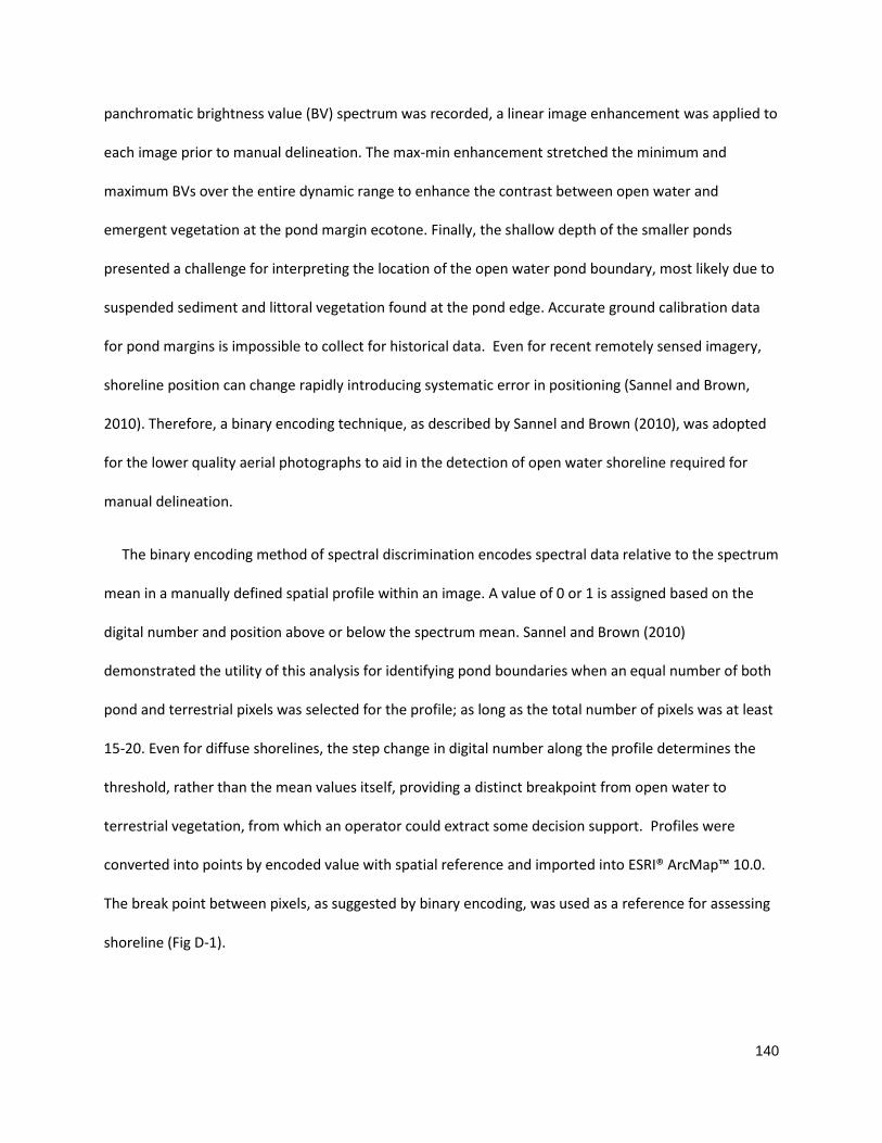
140
panchromatic brightness value (BV) spectrum was recorded, a linear image enhancement was applied to
each image prior to manual delineation. The max-min enhancement stretched the minimum and
maximum BVs over the entire dynamic range to enhance the contrast between open water and
emergent vegetation at the pond margin ecotone. Finally, the shallow depth of the smaller ponds
presented a challenge for interpreting the location of the open water pond boundary, most likely due to
suspended sediment and littoral vegetation found at the pond edge. Accurate ground calibration data
for pond margins is impossible to collect for historical data. Even for recent remotely sensed imagery,
shoreline position can change rapidly introducing systematic error in positioning (Sannel and Brown,
2010). Therefore, a binary encoding technique, as described by Sannel and Brown (2010), was adopted
for the lower quality aerial photographs to aid in the detection of open water shoreline required for
manual delineation.
The binary encoding method of spectral discrimination encodes spectral data relative to the spectrum
mean in a manually defined spatial profile within an image. A value of 0 or 1 is assigned based on the
digital number and position above or below the spectrum mean. Sannel and Brown (2010)
demonstrated the utility of this analysis for identifying pond boundaries when an equal number of both
pond and terrestrial pixels was selected for the profile; as long as the total number of pixels was at least
15-20. Even for diffuse shorelines, the step change in digital number along the profile determines the
threshold, rather than the mean values itself, providing a distinct breakpoint from open water to
terrestrial vegetation, from which an operator could extract some decision support. Profiles were
converted into points by encoded value with spatial reference and imported into ESRI® ArcMap™ 10.0.
The break point between pixels, as suggested by binary encoding, was used as a reference for assessing
shoreline (Fig D-1).

141
To account for the potential uncertainty resulting from human decision making in distinguishing
shoreline from changes in terrestrial community, ten delineation trials for each pond sampled in the
field was performed and the uncertainty, represented by the standard error of the mean surface area,
was calculated for each. To evaluate changes in precision between image types, the number of vertices
per m2 was quantified and compared using a Bartlett test of equal variances. Average m2/vertex
increases slightly with image quality (Fig D-2), but this change was insignificant.
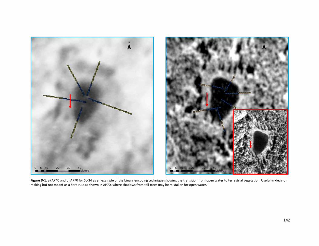
142
Figure D-1: a) AP40 and b) AP70 for SL-34 as an example of the binary encoding technique showing the transition from open water to terrestrial vegetation. Useful in decision making but not meant as a hard rule as shown in AP70, where shadows from tall trees may be mistaken for open water.
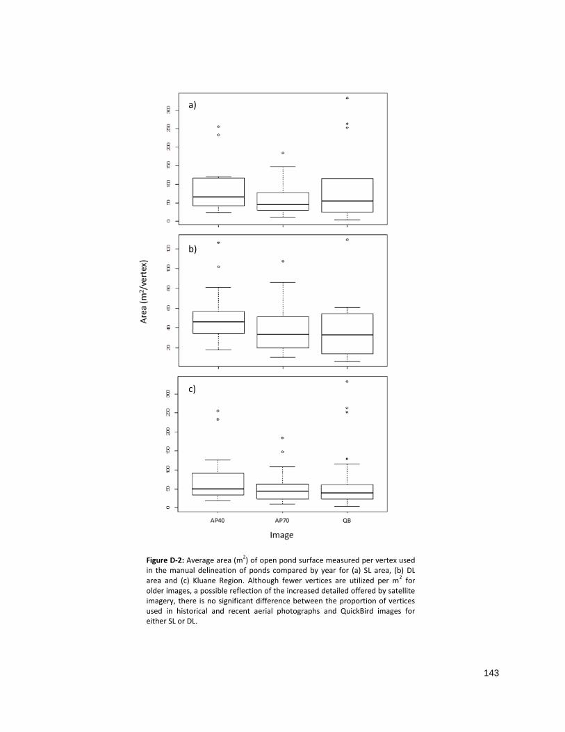
143
a)
b)
c)
Figure D-2: Average area (m2) of open pond surface measured per vertex used
in the manual delineation of ponds compared by year for (a) SL area, (b) DL area and (c) Kluane Region. Although fewer vertices are utilized per m
2 for
older images, a possible reflection of the increased detailed offered by satellite imagery, there is no significant difference between the proportion of vertices used in historical and recent aerial photographs and QuickBird images for either SL or DL.
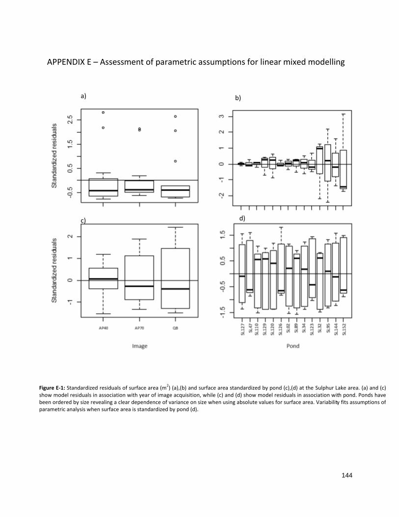
144
APPENDIX E – Assessment of parametric assumptions for linear mixed modelling
a) b)
c) d)
Figure E-1: Standardized residuals of surface area (m2) (a),(b) and surface area standardized by pond (c),(d) at the Sulphur Lake area. (a) and (c)
show model residuals in association with year of image acquisition, while (c) and (d) show model residuals in association with pond. Ponds have been ordered by size revealing a clear dependence of variance on size when using absolute values for surface area. Variability fits assumptions of parametric analysis when surface area is standardized by pond (d).

145
Figure E-2: Standardized residuals of surface area (m2) (a), (b) and surface area standardized by pond (c), (d) at the Dezadeash
Lake area. (a) and (c) show model residuals in association with year of image acquisition, while (c) and (d) show model residuals in association with pond. Ponds have been ordered by size revealing a clear dependence of variance on size when using absolute values for surface area. Variability fits assumptions of parametric analysis when surface area is standardized by pond (d).
a) b)
c) d)
146
APPENDIX F – Construction and validation of comprehensive climate data for the Kluane Region
The nearest weather station is located in the village of Haines Junction, YT (60°45′10″ N, 137°30′24″
W); approximately 50 km from the furthest pond sampled in both sites. Adjusted and homogenized
climate data, created for use in climate research, is available for daily mean surface temperature
(Vincent et al., 2012) and precipitation (Mekis and Vincent, 2011) from the Haines Junction weather
station. The data have been adjusted to address shifts in instrument and recording procedures, in some
cases involving the combination of multiple stations, in order to generate longer time series, which was
the case for precipitation data acquired from Haines Junction. Because of this, several years are missing
from the timeline including an entire decade from 1984 to 1994. Climate data from 1995 to present is
highly unreliable, possessing several missing values and a large number of estimated values.
Climate data is seasonally autocorrelated. Therefore, to predict values, only annual data, calculated
from average monthly data for each year, was used for each weather station. Years with missing
monthly data were omitted, and only time series displaying stochastic behavior were considered; which
was true for both Burwash Landing and City of Whitehorse data. Models were validated by quantifying
disparity between predicted and actual values for Haines Junction. Because precipitation data could not
be predicted with an acceptable degree of uncertainty, City of Whitehorse data was used as it correlated
most closely with the available Haines Junction data. Although a parsimonious model to predict
temperature would exclude Burwash without significant loss of explanatory value, several years were
missing from the Whitehorse data set so both stations were incorporated into the model. In the rare
cases where a complete year was not available for either Whitehorse or Burwash, the value was
interpolated by a three year moving average of Haines Junction Data. Average monthly temperatures
were calculated for Haines Junction along with precipitation for the three weather stations (Fig F-1).

147
Adjusted monthly temperatures for Haines junction were predicted with a residual standard error
of 1.221 on 311 degrees of freedom. Almost all variance in true values were explained by predicted
mean monthly temperature (F2,311 = 3000, p < 0.001, r2 = 0.99,). Predictive power of precipitation was
considerably less, with a residual error of 20.18 and little variance in true values explained (F2,311 = 123.3,
p < 0.001, r2 = 0.23,). Therefore, missing values in adjusted data were replaced with predicted values for
temperature only.
Autocorrelation of monthly time series data was avoided by averaging climate variables across each
year for which all monthly values were available. Durbin Watson tests, evaluation of lagged correlation,
and standardized residuals, verified the independence and normality of both observations and residuals
for each climate model.
The number of missing values in the latter half of the study period was supplemented by also
analyzing Whitehorse climate data, which, although did not prove useful in predicting precipitation,
correlated quite closely with monthly observations. A similar outcome was retrieved from this weather
station (0.81 ±0.36 mm per year, F = 4.902, df = 63, r2 = 0.07), with a disparate, although significant (p <
0.05) change in precipitation when compared to temperature of Haines junction. In both cases, almost
none of the variance is explained by year).
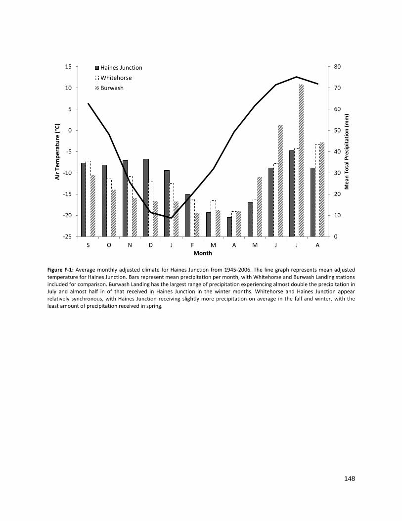
148
Figure F-1: Average monthly adjusted climate for Haines Junction from 1945-2006. The line graph represents mean adjusted temperature for Haines Junction. Bars represent mean precipitation per month, with Whitehorse and Burwash Landing stations included for comparison. Burwash Landing has the largest range of precipitation experiencing almost double the precipitation in July and almost half in of that received in Haines Junction in the winter months. Whitehorse and Haines Junction appear relatively synchronous, with Haines Junction receiving slightly more precipitation on average in the fall and winter, with the least amount of precipitation received in spring.
0
10
20
30
40
50
60
70
80
-25
-20
-15
-10
-5
0
5
10
15
S O N D J F M A M J J A
Me
an T
ota
l Pre
cip
itat
ion
(m
m)
Air
Te
mp
era
ture
(°C
)
Month
Haines Junction
Whitehorse
Burwash