Applications of Geometric Algebra in

Robot Vision

University of Kiel, Cognitive Systems Group

Gerald Sommer

Abstract

In this tutorial paper we will report on our experience in the use of geometricalgebra (GA) in robot vision. The results could be reached in a long term researchprogramme on modelling the perception-action cycle within geometric algebra. Wewill pick up three important applications from image processing, pattern recogni-tion and computer vision. By presenting the problems and their solutions from anengineering point of view, the intention is to stimulate other applications of GA.

1 Introduction

In this paper we want to present a tutorial survey on applications of geometric algebra(GA) in robot vision. We will restrict our scope to results contributed by the Kiel Cogni-tive Systems Group in the last few years. For more details and for getting a wider view onthis topic a visit of the publications on the website http://www.ks.informatik.uni-kiel.deis recommended. Especially the tutorial reports [14] and [17] may be helpful.We will take on an engineer’s viewpoint to give some impression of the need of suchcomplex mathematical framework as geometric algebra for designing robot vision systemsmore easily. In fact, we are using GA as a mathematical language for modelling. Thisincludes the task related shaping of that language itself.

1.1 Robot Vision

The aim of robot vision is to make robots seeing, i.e. to endow robots with visual ca-pabilities comparable to those of human. While contemporary applications of robots arerestricted to industrial artificial environments, the hope is that future generations of robotsare able to cope with real world conditions. The term robot vision indicates a concentra-tion of research activities onto modelling of useful visual architectures. On the other handthe term visual robotics emphasizes the control of robots by visual sensoric information.

1

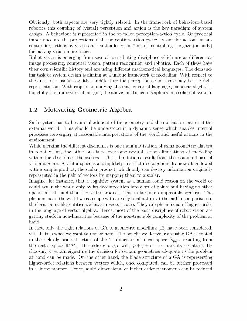
Obviously, both aspects are very tightly related. In the framework of behaviour-basedrobotics this coupling of (visual) perception and action is the key paradigm of systemdesign. A behaviour is represented in the so-called perception-action cycle. Of practicalimportance are the projections of the perception-action cycle: “vision for action” meanscontrolling actions by vision and “action for vision” means controlling the gaze (or body)for making vision more easier.Robot vision is emerging from several contributing disciplines which are as different asimage processing, computer vision, pattern recognition and robotics. Each of these havetheir own scientific history and are using different mathematical languages. The demand-ing task of system design is aiming at a unique framework of modelling. With respect tothe quest of a useful cognitive architecture the perception-action cycle may be the rightrepresentation. With respect to unifying the mathematical language geometric algebra ishopefully the framework of merging the above mentioned disciplines in a coherent system.

1.2 Motivating Geometric Algebra

Such system has to be an embodiment of the geometry and the stochastic nature of theexternal world. This should be understood in a dynamic sense which enables internalprocesses converging at reasonable interpretations of the world and useful actions in theenvironment.While merging the different disciplines is one main motivation of using geometric algebrain robot vision, the other one is to overcome several serious limitations of modellingwithin the disciplines themselves. These limitations result from the dominant use ofvector algebra. A vector space is a completely unstructured algebraic framework endowedwith a simple product, the scalar product, which only can destroy information originallyrepresented in the pair of vectors by mapping them to a scalar.Imagine, for instance, that a cognitive system as a human could reason on the world orcould act in the world only by its decomposition into a set of points and having no otheroperations at hand than the scalar product. This in fact is an impossible scenario. Thephenomena of the world we can cope with are of global nature at the end in comparison tothe local point-like entities we have in vector space. They are phenomena of higher orderin the language of vector algebra. Hence, most of the basic disciplines of robot vision aregetting stuck in non-linearities because of the non-tractable complexity of the problem athand.In fact, only the tight relations of GA to geometric modelling [12] have been considered,yet. This is what we want to review here. The benefit we derive from using GA is rootedin the rich algebraic structure of the 2n -dimensional linear space Rp,q,r resulting fromthe vector space R

p,q,r . The indexes p, q, r with p + q + r = n mark its signature. Bychoosing a certain signature the decision for certain geometries adequate to the problemat hand can be made. On the other hand, the blade structure of a GA is representinghigher-order relations between vectors which, once computed, can be further processedin a linear manner. Hence, multi-dimensional or higher-order phenomena can be reduced

2

to one-dimensional or linear representations. This has not only impact on modelling ofgeometric problems but of stochastic ones also. Therefore, there is need of using GA incontext of higher-order statistics too.In the following sections we want to show the advantages of using GA in three differentareas of robot vision. These are signal analysis, pattern recognition using the paradigmof neural computing, and computer vision. In each case we will emphasize the inherentlimitations of modelling in the classical scheme and the benefits we gain from using GAinstead. In the conclusion section we will give a summary of all these advantages in amore general way.

2 Analysis of Multi-dimensional Signals

Image analysis as a fundamental part of robot vision does not mean to deliver completedescriptions of scenes or to recognize certain objects. This in fact is subject of computervision. Instead, the aim of image analysis is deriving a set of rich features from visualdata for further processing and analysis. In (linear) signal theory we are designing (linearshift invariant) operators which should extract certain useful features from signals. TheFourier transform plays a major role because representations of both operators and im-ages in spectral domain are useful for interpretation.In this section we want to give an overview on our endavours of overcoming a not well-known representation gap in Fourier domain in case of multi-dimensional signals. Infact, the well-known complex valued Fourier transform cannot explicitely represent multi-dimensional phase concepts. The Fourier transform is a global integral transform andamplitude and phase are global spectral representations. More important in practice isthe incompleteness of local spectral representations in multi-dimensional case. This isa representation problem of the Hilbert transform which delivers the holomorphic com-plement of a one-dimensional real valued signal. Therefore, the aim of this section isshowing generalizations of both Fourier and Hilbert transform from the one-dimensionalto the multi-dimensional case which are derived from embeddings into geometric algebra.In that respect two different concepts of the term dimension of a function have to bedistinguished. The first one is the global embedding dimension, which is related to theFourier transform. The second one is the (local) intrinsic dimension, which is related tothe Hilbert transform and which means the degrees of freedom that locally define thefunction.

2.1 Global Spectral Representations

It is well-known that the complex valued Fourier transform, F c ∈ C ,

F c(u) = F c {f(x)} =

∫f(x) exp(−j2πux) dNx (1)

3

enables computing the spectral representations amplitude Ac(u) and phase Φc(u) ,

Ac(u) = |F c(u)| (2a)

Φc(u) = arg (F c(u)) , (2b)

of the real valued N -dimensional (ND) function f(x) , x ∈ RN . Although it is common-

sense that the phase function is representing the structural information of the function,there is no way in complex domain to explicitly access to ND structural information forN > 1 . This problem is related to the impossibility of linearly representing symmetriesof dimension N > 1 in complex domain.In fact, the Fourier transform in 1D case can be seen as a way to compute the integralover all local symmetry decompositions of the function f(x) into an even and an oddcomponent according to

f(x) = fe(x) + fo(x) (3)

F c(u) = F ce (u) + F c

o (u). (4)

This results from the Euler decomposition of the Fourier basis functions

Qc(u, x) = exp(−j2πux) = cos(2πux) − j sin(2πux). (5)

In case of 2D complex Fourier transform the Euler decomposition of the basis functions

Qc(u,x) = exp(−j2πux) = exp(−j2πux) exp(−j2πvy) (6)

corresponds to a signal decomposition into products of symmetries with respect to coor-dinate axes,

F c(u) = F cee(u) + F c

oo(u) + F coe(u) + F c

eo(u). (7)

But this concept of line symmetry is partially covered in complex domain because of thelimited degrees of freedom. If F c

R(u) and F cI (u) are the real and imaginary components

of the spectrum, respectively, F c(u) = F cR(u) + jF c

I (u) , then

F cR(u) = F c

ee(u) + F coo(u) , F c

I (u) = F ceo(u) + F c

oe(u). (8)

If we consider the Hartley transform [10] as a real valued Fourier transform, F r(u), thenalso in 1D case the components F r

e (u) and F ro (u) are totally covered in F r ∈ R . This

observation supports the following statement [6]. Given a real valued function f(x) ,x ∈ R

N , then all its global decompositions into even and odd symmetry components withrespect to coordinate axes is given by the Clifford valued Fourier transform F Cl ∈ R2N ,

F Cl(u) = FCl {f(x)} =

∫

RN

f(x)N∏

k=1

exp(−ik2πukxk) dNx. (9)

4

Figure 1: Left: basis functions of the complex 2D Fourier transform. Right: basis functions of

the quaternionic 2D Fourier transform. Only the even/even-even part is shown each.

In 2D case the Fourier transform has to be quaternionic, F q ∈ H ,

F q(u) = F q {f(x)} =

∫

R2

f(x) exp(−i2πux) exp(−j2πvy) d2x (10)

with

Qq(u,x) = exp(−i2πux) exp(−j2πvy). (11)

Because

F q(u) = FqR(u) + iF

qI (u) + jF

qJ (u) + kF

qK(u) (12a)

F q(u) = F qee(u) + F q

oe(u) + F qeo(u) + F q

oo(u), (12b)

all symmetry combinations are explicitely accessible by one real and three imaginaryparts. As figure 1 visualizes, the basis functions according to (11) are intrinsically two-dimensional in contrast to those of (6) and, thus, they can represent 2D structural in-formation. This can also be seen in the polar representation of the quaternionic Fouriertransform [6], where φ and θ represent each a 1D phase, ψ is a 2D phase.

F q(u) = |F q(u)| exp (iφ(u)) exp (kψ(u)) exp (jθ(u)) . (13)

2.2 Local Spectral Representations

As local spectral representations we call functions of local energy, e(x) , (or amplitude,a(x) =

√e(x)) , and local phase, φ(x) ,

e(x) = f 2(x) + f 2H(x) (14a)

5

φ(x) = arg (fA(x)) , (14b)

which are derived from a complex valued extension, fA(x) , of a real 1D function f(x) byan operator A ,

fA(x) = A{f(x)} = f(x) + jfH(x). (15)

In signal theory fA(x) is called analytic signal and fH(x) is derived from f(x) by a localphase shift of −π

2, which is gained by the Hilbert transform, H , of f(x) ,

fH(x) = H{f(x)} . (16)

This corrresponds in complex analysis to compute the holomorphic complement of f(x)by solving the Laplace equation. In complex Fourier domain the Hilbert transform reads

H(u) = −ju

|u|, (17)

thus, the operator of the analytic signal is given by the frequency transfer function

A(u) = 1 +u

|u|. (18)

The importance of the analytic signal in signal analysis results from the evaluation ofthe local spectral representations, equations (14a) and (14b): If the local energy exceedssome threshold at x , then this indicates an interesting location. The evaluation of thelocal phase enables a qualitative signal interpretation with respect to a mapping of thesignal to a basis system of even and odd symmetry according to equation (3). For moredetails see [17]. In image processing we can interprete lines as even symmetric structuresand edges as odd symmetric ones, both of intrinsic dimension one. But in images we haveas an additional unknown the orientation of lines or edges. Hence, the operators A orH , respectively, should be rotation invariant. Although the analytic signal is also usedin image processing since one decade, only by embedding into GA, this problem could besolved.Simply to take over the strategy described in section 2.1 from global to local domain isnot successful. The quaternionic analytic signal [7], which is derived from a quaternionicHilbert transform delivers no rotation invariant local energy. Hence, the applied conceptof line symmetry cannot succeed in formulating isotropic operators.Instead, an isotropic generalization of the Hilbert transform in case of a multidimensionalembedding of a 1D function can be found by considering point symmetry in the imageplane. This generalization is known in Clifford analysis [3] as Riesz transform.The Riesz transform of a real ND function is an isotropic generalization of the Hilberttransform for N > 1 in a (N + 1)D space. In Clifford analysis, i.e. an extension of thecomplex analysis of 1D functions to higher dimensions, a real ND function is consideredas a harmonic potential field, f(x) , in the geometric algebra RN+1 . The Clifford valuedextension of f(x) is called monogenic extension and is located in the hyperplane where

6

f M

e 1

ϕ

e3

e2

θ

Figure 2: The phase decomposition of a monogenic signal expressing symmetries of a local i1D

structure embedded in R3 . The great circle is passing |f M |e 3 and f M defines the orientation

of a complex plane in R3 .

the (N + 1)th component, say s , vanishes. It can be computed by solving the (N + 1)DLaplace equation of the corresponding harmonic potential as a boundary value problemof the second kind for s = 0 (see [8]).Let us consider the case of a real 2D signal, f(x) , represented as e3 -valued vector fieldf(x) = f(x)e3 in the geometric algebra R3 . Then in the plane s = 0 a monogenic signalfM exists [9],

fM(x) = f(x) + fR(x), (19)

where fR(x) is the vector of the Riesz transformed signal. In our considered case themonogenic signal is a generalization of the analytic signal, equation (15), for embeddingan intrinsically 1D function into a 2D signal domain. Similarly the Riesz transform withthe impulse response

hR(x) =xe3

2π|x|3= −

x

2π|x|3e31 +

y

2π|x|3e23 (20)

and the frequency transfer function

HR(u) =u

|u|I−12 , I2 = e12 (21)

generalizes all properties known from the Hilbert transform to 2D.The local energy, derived from the monogenic signal is rotation invariant. Furthermore,the phase generalizes to a phase vector, whose one component is the normal phase angleand the second component represents the orientation angle of the intrinsic 1D structurein the image plane. Hence, the set of local spectral features is augmented by a feature of

7

geometric information, that is the orientation. In figure 2 can be seen how the complexplane of the local spectral representations rotates in the augmented 3D space. This resultsin an elegant scheme of analyzing intrinsically 1D (i1D) structures in images.Sofar, we only considered the solution of the Laplace equation for s = 0. The extension tos > 0 results in a set of operators, called Poisson kernels and conjugated Poisson kernels,respectively, which not only form a Riesz triple with quadrature phase relation as thecomponents in equation (19), but transform the monogenic signal into a representationwhich is called scale-space representation. In fact, the s -component is a scale-spacecoordinate. A scale-space is spanned by (x, s) . This is a further important result becausefor nearly 50 years only the Gaussian scale-space, which results as a solution of the heatequation, has been considered as scale-space for image processing. One advantage of thePoisson scale-space in comparison to the Gaussian scale-space is its alibity to naturallyembed the complete local spectral analysis into a scale-space theory. Regrettably, thisnice theory derived from Clifford analysis framework is relevant only for i1D signals, yet.The extension to i2D structures in images like curved lines/edges, crosses or any othermore general structure will be matter of future research. Nevertheless, in [9] a so-calledstructure multivector is proposed from which a rich set of features can be derived for aspecial model of an i2D structure.

3 Knowledge Based Neural Computing

Neural nets are computational tools for learning certain competences of a robot visionsystem within the perception-action cycle. A net of artificial neurons as primitive pro-cessing units can learn for instance classification, function approximation, prediction orcontrol. Artificial neural nets are determined in their functionality by the kind of neuronsused, their topological arrangement and communication, and the weights of the connec-tions. By embedding neural computing into the framework of GA, any prior algebraicknowledge can be used for increasing the performance of the neural net. The main benefitwe get from this approach is constraining the decision space and, thus, preventing thecurse of dimensionality. From this can follow faster convergence of learning and increasedgeneralization capability. For instance, if the task is learning the parameters of a trans-formation group from noisy data, then noise does not follow the algebraic constraints ofthe transformation group and will not be learned.In subsection 3.1 we will consider such type of problems under orthogonal constraints.Another advantage of embedding neural computing into geometric algebras is relatedto learning of functions. Neural nets composed by neurons of perceptron type - this isthe type of neurons we will consider here - are able to learn nonlinear functions. If thenonlinear problem at hand is transformed in an algebraic way to a linear one, then learn-ing becomes much easier and with less ressources. We will consider such problems incase of manifold learning in subsection 3.1 and in case of learning decision boundaries insubsection 3.2. For more details see [17].

8

3.1 The Spinor Clifford Neuron

In this subsection we will consider the embedding of perceptron neurons into a chosengeometric algebra. The output, y , of such neuron for a given input vector x and a weightvector w, x,w ∈ R

n , is given by

y = g (f(x;w)) . (22)

The nonlinear function g : R −→ R is called activation function. It shall be omitted inthe moment, say, by setting it to the identity. More important is the propagation functionf : R

n −→ R ,

f(x) =n∑

i=1

wixi + θ, (23)

where θ ∈ R is a bias (threshold). Obviously, one single neuron can learn a linear function,represented by equation (23), as linear regression task by minimizing the sum of squarederrors over all samples (xj, rj) from a sufficiently composed sample set (universe). Weassume a supervised training scheme where rj ∈ R is the requested output of the neuron.By arranging a certain number of neurons in a single layer fully connected to the inputvector x , we will get a single layer perceptron network (SLP). A SLP obviously enablestask sharing in a parallel fashion and, hence, can perform a multi-linear regression. Ifx,y ∈ R

n , then

y = Wx (24)

is representing a linear transformation by the weight matrix W .After introducing the computational principles of a real valued neuron, we will extendnow our neuron model by embedding it into the GA Rp,q, p + q = n, see [5]. Hence, forx,w, θ ∈ Rp,q the propagation function f : Rp,q −→ Rp,q reads

f(x) = wx + θ (25)

where wx should be the geometric product instead of the scalar product of equation(23). A neuron with a propagation function according to equation (25) is called a Cliffordneuron. The superiority of equation (25) over equation (23) follows from explicitly intro-ducing a certain algebraic model as constraint by choosing Rp,q for learning the weightmatrix of equation (24) instead of additionally learning the required constraints. It isobviously more advantageous to use a model than to perform its simulation. This leadsin addition to a reduction of the required resources (neurons, connections). By explicitlyintroducing algebraic constraints, statistical learning will become a simpler task.We will further extend our model. If the weight matrix W in equation (24) is repre-senting an orthogonal transformation, we can introduce the constraint of an orthogonaltransformation group. This is done by embedding the propagation function now intoR

+p,q . Instead of equation (25) we get for f : R

+p,q −→ R

+p,q :

f(x) = wxw + θ. (26)

9

We will call a neuron with such propagation function a spinor Clifford neuron because thespinor product of the input vector with one weight vector is computed. The representationof an orthogonal transformation by a spinor [12] has several computational advantagesin comparison to a matrix representation which should not be explicitly discussed here.It should only be mentioned that one single spinor Clifford neuron is sufficient to learnany transformation group if the right algebra Rp,q is chosen where this transformationgroup becomes a spin group. To mention one extreme example, in [4], the learning of thecross-ratio by one spinor Clifford neuron in R1,2, i.e. the conformal model of the complexplane, has been reported. The neuron had to learn that Mobius transformation as specialconformal transformation which keeps the cross-ratio of four points in the complex planeR0,1 invariant. But in contrast to R0,1 , in R1,2 the Mobius transformation is an orthogonalone.

3.2 The Hypersphere Neuron

In subsection 3.1 we neglected the activation function in describing our algebraic neuronmodels. This is possible if a kind of function learning is the task at hand. In case of aclassification task the non-linear activation function is mandatory to complete the percep-tron to a non-linear computing unit which in the trained state represents a linear decisionboundary in R

n . The decision boundary enables solving a 2-class decision problem bydividing the sample space in two half-spaces. Regrettably, the higher the dimension n

of the feature vectors, the less likely a 2-class problem can be treated with a linear hy-perplane of R

n . Therefore, parallel (SLP) or sequential (MLP - multilayer perceptron)compositions of neurons are necessary for modelling non-linear decision boundaries.One special case is a hypersphere decision boundary. This can be only very inefficientlymodelled by using perceptrons. But spheres are the geometric basis entities of conformalgeometry. That is, in conformal geometry we can operate on hyperspheres in a linearmanner just as operating on points in Euclidean geometry (points are the basis entitiesof Euclidean geometry).In the last few years the conformal geometric algebra (GA) Rp+1,q+1 [13] became an im-portant embedding framework of different problems relevant to robot vision because ofseveral attractive properties. We will come back to that point in section 4. As mentionedabove, the conformal group C(p, q) , which is highly non-linear in R

p,q transforms to arepresentation which is isomorphic to the orthogonal group O(p + 1, q + 1) in Rp+1,q+1 .Second, a subspace of the conformal space R

n+1,1 which is called horosphere, Nne , is a

non-Euclidean model of the Euclidean space Rn with the remarkable property of metri-

cal equivalence. This is the property we want to exploit for constructing the hypersphereneuron. Here we need in fact only the vector space R

n+1,1 = 〈Rn+1,1〉1 of the CGA.Any point x ∈ R

n transforms to a point x ∈ Rn+1,1 with x2 = 0. That is, points are

represented as null vectors on the horosphere. Because hyperspheres are the basis entitiesof R

n+1,1 , a point x can be seen as a degenerate hypersphere s with radius zero.Let be x,y ∈ R

n two points with Euclidean distance d(x,y) = ‖x − y‖ and let be

10

−1 0 1

−1.5

−1

−0.5

0

0.5

1

1.5

1st principal component 2n

d pr

inci

pal c

ompo

nent

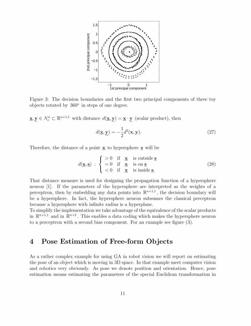
Figure 3: The decision boundaries and the first two principal components of three toyobjects rotated by 360o in steps of one degree.

x,y ∈ Nne ⊂ R

n+1,1 with distance d(x,y) = x · y (scalar product), then

d(x,y) = −1

2d2(x,y). (27)

Therefore, the distance of a point x to hypersphere s will be

d(x, s) :

> 0 if x is outside s

= 0 if x is on s

< 0 if x is inside s.

(28)

That distance measure is used for designing the propagation function of a hypersphereneuron [1]. If the parameters of the hypersphere are interpreted as the weights of aperceptron, then by embedding any data points into R

n+1,1 , the decision boundary willbe a hypersphere. In fact, the hypersphere neuron subsumes the classical perceptronbecause a hypersphere with infinite radius is a hyperplane.To simplify the implementation we take advantage of the equivalence of the scalar productsin R

n+1,1 and in Rn+2 . This enables a data coding which makes the hypersphere neuron

to a perceptron with a second bias component. For an example see figure (3).

4 Pose Estimation of Free-form Objects

As a rather complex example for using GA in robot vision we will report on estimatingthe pose of an object which is moving in 3D space. In that example meet computer visionand robotics very obviously. As pose we denote position and orientation. Hence, poseestimation means estimating the parameters of the special Euclidean transformation in

11

space by observations of the rigid body motion in the image plane. Pose estimation is abasic task of robot vision which can be used in several respects as part of more complextasks as visual tracking, homing or navigation. Although there is plenty of solutions overthe years, only CGA [13] gives a framework which is adequate to the problem at hand[15].The diversity of approaches known sofar results from the hidden complexity of the prob-lem. Estimation of the parameters of the special Euclidean transformation, which iscomposed by rotation and translation, has to be done in a projective scenario. But thecoupling of projective and special Euclidean transformations, both with non-linear repre-sentations in the Euclidean space, results in a loss of the group properties. Another pointis how to model the object which serves as reference. In most cases a set of point featuresis used. But this does not enable to exploit internal constraints contained in higher orderentities as lines, planes, circles, etc. Finally, it can be distinguished between 2D and 3Drepresentations of either model data and measurement data.To be more specific, the task of pose estimation is the following: Given a set of geomet-ric features represented in an object centered frame and given the projections of thesefeatures onto the image plane of a camera, then, for a certain parametrized projectionmodel, determine the parameters of the rigid body motion between two instances of anobject centered frame by observations in a camera centered frame.In our scenario we are assuming a 2D-3D approach, i.e. having 2D measurement datafrom a calibrated full perspective monocular camera and 3D model data. As model weare taking either a set of geometric primitives as points, lines, planes, circles or spheres,or more complex descriptions as a kinematic chain (coupled set of piecewise rigid parts)or free-form curves/surfaces given as CAGD-model. From the image features we are pro-jectively reconstructing lines or planes in space. Now the task is to move the referencemodel in such a way that the spatial distance of the considered object features to theprojection rays/planes becomes zero. This is an optimization task which is done by agradient descent method on the spatial distance as error measure. Hence, we preventminimizing any error measure directly on the manifold.

4.1 Pose Estimation in Conformal Geometric Algebra

We cannot introduce here the conformal geometric algebra [13] because of limited space.There is plenty of good introductions, see e.g. the PhD thesis [15] with respect to anextended description of pose estimation in that framework.We are using the CGA R4,1 of the Euclidean space R

3 . If R3 is spanned by the unit

vectors ei , i = 1, 2, 3, then R4,1 is the algebra of the augmented space R4,1 = R

3,0 ⊕R1,1

with the additional basis vectors eo (representing the point at origin) and e (representingthe point at infinity). The basis {eo, e} constitutes a null basis. From this follows thatthe representation of geometric entities by null vectors is the characteristic feature of thatspecial conformal model of the Euclidean space.The advantages we can profit from within our problem are the following. First, R4,1

12

constitutes a unique framework for affine, projective and Euclidean geometry. If R3,0 isthe geometric algebra of the 3D Euclidean space and R3,1 is that one of the 3D projectivespace, then we have the following relations between these linear spaces:

R3,0 ⊂ R3,1 ⊂ R4,1.

Because the special Euclidean transformation is a special affine transformation, we canhandle either kinematic, projective or metric aspects of our problem in the same algebraicframe. Higher efficiency is reached by simply transforming the representations of thegeometric entities to the respective partial space.Second, the special Euclidean group SE(4, 1) is a subgroup of the conformal group C(4, 1), which is an orthogonal group in R

+4,1 . Hence, the members of SE(4, 1) , which we call

motors, M , are spinors representing a general rotation. Any entity u ∈ R4,1 will betransformed by the spinor product,

u′ = MuM. (29)

Let be R a rotor as representation of pure rotation and let be T another rotor, calledtranslator, representing translation in R

3 , then any g ∈ SE(4, 1) is given by the motor

M = TR (30)

with R,T,M ∈ R+4,1 . Motors have some nice properties. They concatenate multiplica-

tively. If e.g. M = M2M1 , then

u′′ = MuM = M2u′M2 = M2M1uM1M2. (31)

Furthermore, motors are linear operations (as used also in context of spinor Cliffordneurons). That is, we can exploit the outermorphism [11], which is the preservation ofthe outer product under linear transformation.This leads directly to the third advantage of CGA. The incidence algebra of projectivegeometry generalizes in CGA. If s1, s2 ∈ 〈R4,1〉1 are two spheres, then their outer productis a circle, z ∈ 〈R4,1〉2 ,

z = s1 ∧ s2. (32)

If the circle is undergoing a rigid motion, then

z′ = MzM = M(s1 ∧ s2)M = Ms1M ∧ Ms2M = s′1 ∧ s′2. (33)

In very contrast to the (homogeneously extended) Euclidean space, we can handle therigid body motion not only as linear transformation of points but of any entities derivedfrom points or spheres. These entities are no longer only set conceptions as subspaces ina vector space but algebraic entities. This enables also to handle any free-form object asone algebraic entity which can be used for gradient based pose estimation in the samemanner as points. That is a real cognitive approach to the pose problem.

13

Finally, we can consider the special Euclidean group SE(4, 1) as Lie group and are able toestimate the parameters of the generating operator of the group member. This approachleads to linearization and very fast iterative estimation of the parameters. Although thisapproach is also applicable to points in an Euclidean framework, in CGA it is applicableto any geometric entity built from points or spheres.The generating operator of a motor is called twist, Ψ ∈ se(4, 1) . The model of the motoras a Lie group member changes in comparison to equation (30) to

M = TRT. (34)

This equation, which expresses a general rotation as Lie group member in R4,1 , canbe easily interpreted. The general rotation is performed as normal rotation, R , in therotation plane l ∈ 〈R3〉2 , which passes the origin, by an angle θ ∈ R , after correctingthe displacement t ∈ 〈R3〉1 of the rotation axis l∗ ∈ 〈R3〉1 from the origin with help of

the translator T . Finally, the displacement has to be reconstructed by the translator T .From this follows equation (34) in terms of the parameters of the rigid body motion inR3 ,

M = exp

(et

2

)exp

(−

θ

2l

)exp

(−

et

2

). (35)

This factorized representation can be compactly written as

M = exp

(−

θ

2Ψ

). (36)

Here

Ψ = l + e(t · l) (37)

is the twist of rigid body motion. Geometrically interpreted is the twist representing theline l ∈ 〈R4,1〉2 around which the rotation is performed in R4,1 .Now we return to our problem of pose estimation. The above mentioned optimizationproblem is nothing else as a problem of minimizing the spatial distance of e.g. a pro-jection ray to a feature on the silhouette of the reference model. If this distance is zero,then a certain geometric constraint is fulfilled. These constraints are either collinarity orcoplanarity for points, lines and planes, or tangentiality in case of circles or spheres.For instance, the collinearity of a point x ∈ 〈R4,1〉1 , after beeing transformed by themotor M , with a projection line lx is written as their vanishing commutator product,

(MxM) × lx = 0. (38)

This equation has to be written in more details to see its coupling with the observationof a point x in the image plane of the camera:

λ((MxM) × (e ∧ (O ∧ x))

)· e+ = 0. (39)

14

This in fact is the complete pose estimation problem written as a symbolic dense butnevertheless algebraic correct equation. The outer product O ∧ x of the image pointx with the optical center O of the camera results in the projection ray representationin projective space R3,1 . By wedging it with e , we transform the projection ray tothe conformal space R4,1 , hence, lx = e ∧ O ∧ x . Now the collinearity constraint canbe computed in R4,1 . Finally, to assign the constraint an Euclidean distance zero, theexpression has to be transformed to the Euclidean space 〈R3〉1 by computing the innerproduct with the basis vector e+ which is derived from the null basis and by scaling withλ ∈ R . In reality the commutator product will take on a minimum as a result of theoptimization process.

4.2 Twist Representations of Free-form Objects

Sofar we only considered the pose estimation problem on the base of modelling a rigidobject by a set of different order geometric entities. In robotics exists another importantobject model which is piecewise rigid. A kinematic chain is the formalization of severalrigid bodies coupled by either revolute or prismatic joints. If pose estimation is applied toobservatons of e.g. a robot arm for controlling grasping movements, this is the adequatemodel. Each of the parts of an arm is performing movements in mutual dependence.Hence, the motion of the j -th joint causes also motions of the preceding ones. If uj ∈ R4,1

is a geometric entity attached to the j -th segment, e.g. a fingertip, its net displacementcaused by a motor M , represented in the (fixed) base coordinate system, is given by

u′

j = M(M1...MjujMj...M1)M. (40)

Here, the motors Mi are representing the constrained motion of the i -th joint.While in the homogeneous space R

4 this equation is limited to points as moving entitiesand in the framework of the motor algebra [2] lines and planes can be considered inaddition, there is no such restriction in CGA.The idea of the kinematic chain can be further generalized to a generator of free-formshape. We will consider the trajectory caused by the motion of the entity u in space asthe orbit of a multi-parameter Lie group of SE(4, 1) . This multi-parameter Lie grouprepresents a possibly very complex general rotation in R4,1 which is generated by a set ofnested motors, contributing each with its own constrained elementary general rotation. Ifthe entity u would be a point, then the orbit can be a space curve, a surface or a volume.But u can also be of higher order (e.g. a tea pot). Hence, the generated orbit may be ofany complexity.This kinematic model of shape in CGA [16] has not been known before, although there isa long history of relating kinematics and geometry, e.g. with respect to algebraic curves,or of the geometric interpretation of Lie groups.The mentioned generalization of the model of a kinematic chain is twofold. First, therotation axes of the motors must not be positioned at the periphery of the shape but maybe (virtually) located anywhere. Second, several different oriented axes may be fixed at

15

the same location.The principle of constructing higher order 3D curves or surfaces as orbit of a point whichis controlled by only a few coupled twists as generators is simple. Let be xz an arbitrarypoint on a circle z , that is xz · z = 0, and let be M(l; θ) the corresponding motor, thenfor all θ ∈ [0, ..., 2π]

x(1)z = MxzM (41)

generates the circle z . If the motor is representing a pure translator, then any arbitraryoriented line l will be generated. Such primitive curves will be called 3D-1twist curves.By coupling a second twist to the first one, either a 3D-2twist curve or surface will begenerated. In fact, already this simple system has a lot of degrees of freedom which enablegenerating quite different figures [15]. This can be seen by the following equation:

x(2)c = M2M1xcM1M2 (42)

with

Mi(li; λi, θi) = exp

(−

λiθi

2Ψi

), (43)

Here λi ∈ R is the ratio of the angular frequency, θi ∈ [α1, ..., α2] is the angular segmentwhich is covered by θi and finally Ψi defines the position and orientation of the generalrotation axis li and the type of motion, that is rotation-like, translation-like, or a mixedform.Finally, the twist model of a closed shape is equivalent to the well-known Fourier repre-sentation, we started with this survey [17]. Since the Fourier series expansion of a closed3D curve C(φ) can be interpreted as the action of an infinite set of rotors, R

φk , fixed at

the origin of 〈R3〉1 , onto phase vectors pk , there is no need of using CGA. A plane closedcurve is given by

C(φ) = limN→∞

N∑

k=−N

pk exp

(2πkφ

Tl

)= lim

N→∞

N∑

k=−N

RφkpkR

φk (44)

The phase vectors pk are the Fourier series coefficients. Instead of the imaginary unitof the harmonics, the unit bivector l ∈ R3, l

2 = −1 , is used which defines the rotationplane of the phase vectors. Based on the assumption that any closed 3D curve can bereconstructed from three orthogonal projections, a spatial curve is represented by

C(φ) = limN→∞

3∑

m=1

N∑

k=−N

pmk exp

(2πkφ

Tlm

). (45)

This scheme can be extended to free-form surfaces as well and has been used for poseestimation in the presented framework. In that respect the inverse Fourier transform ofdiscretized curves/surfaces was applied. The necessary transformation of the Euclidean

16

15 18 21

9

1 3 8

10 13

Figure 4: Regularization of iterative pose estimation by Fourier representation (numbers indi-

cate the iteration steps).

Fourier representation, CE(φ) , to a conformal one, CC(φ) , can simply be done by thefollowing operation:

CC(φ) = e ∧ (CE(φ) + e−) (46)

where e− stands for the homogeneous coordinate of the projective space R3,1 and wedgingwith e again realizes the transformation from R3,1 to R4,1 .One advantage of using the Fourier interpretation of the twist approach in pose estimationis the possibility of regularizing the optimization in case of non-convex objects. This isdemonstrated in figure (4). During the iteration process, which needs for that object onlya few milliseconds, successively more Fourier coefficients are used. Hence, getting stuckin local minima is prevented.The presented methods used in pose estimation clearly demonstrate the strength of theapplied algebraic model of conformal geometric algebra.

5 Conclusions

We have demonstrated the application of geometric algebra as universal mathematicallanguage for modelling in robot vision. Here we will summarize some general conclusions.First, GA supports generalizations of representations. In section 4 we used the stratifi-cation of spaces of different geometry. This enables simple switching between differentaspects of a geometric entity. Instead of points, in certain GA as CGA, higher order enti-ties take on the role of basis entities from which object concepts with algebraic propertiescan be constructed. We have shown that kinematics, shape theory and Fourier theory areunified in the framework of CGA. Besides, in section 2 we could handle multi-dimensionalfunctions in a linear signal theory.Second, the transformation of non-linear problems to linear ones is another importantadvantage. This could be demonstrated in all presented application fields. In learning

17

theory this enables designing algebraically constrained knowledge based neural nets.Third, GA is a mathematical language which supports symbolic dense formulations withalgebraic meaning. We are able to lift up representations where besides the above men-tioned qualitative aspects also reduced computational complexity results. This is impor-tant in real-time critical applications as robot vision.We can state that the progress we made in robot vision could only be possible on the baseof using geometric algebra and this enforces its use also in other application fields.

6 Acknowledgements

We acknowledge the European Community, Deutsche Forschungsgemeinschaft and Stu-dienstiftung des deutschen Volkes for supporting the research which is reported in thispaper. Especially contributions of Thomas Bulow, Michael Felsberg, Sven Buchholz,Vladimir Banarer, Bodo Rosenhahn and Christian Perwass contributed to the reportedresults. Our thanks are also to Prof. Hitzer, Prof. Nagaoka and Dr. Ishi for organizingthe stimulating conference in Kyoto.

References

[1] V. Banarer, C. Perwass, and G. Sommer. The hypersphere neuron. In Proc. 11th

European Symposium on Artificial Neural Networks, ESANN 2003, Bruges, pages469–474. d-side publications, Evere, Belgium, 2003.

[2] E. Bayro-Corrochano, K. Daniilidis, and G. Sommer. Motor algebra for 3d kinemat-ics: The case of hand-eye calibration. Journal of Mathematical Imaging and Vision,13:79–100, 2000.

[3] F. Brackx, R. Delanghe, and F. Sommen. Clifford Analysis. Pitman Advanced Publ.Program, Boston, 1982.

[4] S. Buchholz and G. Sommer. Learning geometric transformations with Clifford neu-rons. In G. Sommer and Y. Zeevi, editors, 2nd International Workshop on Algebraic

Frames for the Perception-Action Cycle, AFPAC 2000, Kiel, volume 1888 of LNCS,pages 144–153. Springer-Verlag, 2000.

[5] S. Buchholz and G. Sommer. Introduction to neural computation in Clifford algebra.In G. Sommer, editor, Geometric Computing with Clifford Algebras, pages 291–314.Springer-Verlag, Heidelberg, 2001.

[6] T. Bulow. Hypercomplex spectral signal representations for the processing and anal-ysis of images. Technical Report Number 9903, Christian-Albrechts-Universitat zuKiel, Institut fur Informatik und Praktische Mathematik, August 1999.

18

[7] T. Bulow and G. Sommer. Hypercomplex signals - a novel extension of the ana-lytic signal to the multidimensional case. IEEE Transactions on Signal Processing,49(11):2844–2852, 2001.

[8] M. Felsberg. Low-level image processing with the structure multivector. TechnicalReport Number 0203, Christian-Albrechts-Universitat zu Kiel, Institut fur Informatikund Praktische Mathematik, Marz 2002.

[9] M. Felsberg and G. Sommer. The monogenic signal. IEEE Transactions on Signal

Processing, 49(12):3136–3144, 2001.

[10] R.V.L. Hartley. A more symmetrical Fourier analysis applied to transmission prob-lems. Proc. IRE, 30:144–150, 1942.

[11] D. Hestenes. The design of linear algebra and geometry. Acta Appl. Math., 23:65–93,1991.

[12] D. Hestenes, H. Li, and A. Rockwood. New algebraic tools for classical geometry.In G. Sommer, editor, Geometric Computing with Clifford Algebras, pages 3–23.Springer-Verlag, Heidelberg, 2001.

[13] H. Li, D. Hestenes, and A. Rockwood. Generalized homogeneous coordinates forcomputational geometry. In G. Sommer, editor, Geometric Computing with Clifford

Algebras, pages 27–59. Springer-Verlag, Heidelberg, 2001.

[14] C. Perwass and D. Hildenbrand. Aspects of geometric algebra in euclidean, pro-jective and conformal space. Technical Report Number 0310, Christian-Albrechts-Universitat zu Kiel, Institut fur Informatik und Praktische Mathematik, September2003.

[15] B. Rosenhahn. Pose estimation revisited. Technical Report Number 0308, Christian-Albrechts-Universitat zu Kiel, Institut fur Informatik und Praktische Mathematik,September 2003.

[16] B. Rosenhahn, C. Perwass, and G. Sommer. Free-form pose estimation by using twistrepresentations. Algorithmica, 38:91–113, 2004.

[17] G. Sommer. The geometric algebra approach to robot vision. Technical ReportNumber 0304, Christian-Albrechts-Universitat zu Kiel, Institut fur Informatik undPraktische Mathematik, September 2003.

19