Embed Size (px)
Citation preview
Applications of Computational Geometry to
Computer Aided Design, Computer Graphics and
Computer Vision
John Edgar Congote Calle
March 2009

2
Applications of Computational Geometry toComputer Aided Design, Computer Graphics and
Computer Vision
Student: John Edgar Congote CalleAdvisor: Prof. Oscar E. Ruiz
School of EngineeringEAFIT UniversityMedellın, Colombia
Submitted in partial fulfillment of the requirements for a
Masters of Science degree in Engineering from the School of
Engineering, EAFIT University
March, 2009

4

Acknowledgements
This work has been partially supported by the Colombian Council for Scienceand Technology -Colciencias-. The Spanish Administration agency CDTI, underproject CENIT-VISION 2007-1007. VICOMTech Institute and CAD/CAM/CAELaboratory - EAFIT University. The bunny model is courtesy of the StanfordComputer Graphics Laboratory and Middlebury College for the stereo visiondata set.
5

6

Contents
1 Introduction 9
2 Surface Triangulation 112.1 Context . . . . . . . . . . . . . . . . . . . . . . . . . . . . . . . . 112.2 Abstract . . . . . . . . . . . . . . . . . . . . . . . . . . . . . . . . 132.3 Introduction . . . . . . . . . . . . . . . . . . . . . . . . . . . . . . 132.4 Literature Review . . . . . . . . . . . . . . . . . . . . . . . . . . 142.5 Curvature Measurement in Parametric Surfaces . . . . . . . . . . 162.6 Methodology . . . . . . . . . . . . . . . . . . . . . . . . . . . . . 18
2.6.1 Calculation of F−1 . . . . . . . . . . . . . . . . . . . . . . 182.6.2 Star Algorithm . . . . . . . . . . . . . . . . . . . . . . . . 182.6.3 Sprinkle Algorithm . . . . . . . . . . . . . . . . . . . . . . 192.6.4 A Pseudo - Delaunay Triangulation . . . . . . . . . . . . 20
2.7 Results . . . . . . . . . . . . . . . . . . . . . . . . . . . . . . . . . 222.8 Conclusions and Future Work . . . . . . . . . . . . . . . . . . . . 23
3 Adaptative Cubical Grid 293.1 Context . . . . . . . . . . . . . . . . . . . . . . . . . . . . . . . . 293.2 Abstract . . . . . . . . . . . . . . . . . . . . . . . . . . . . . . . . 313.3 Introduction . . . . . . . . . . . . . . . . . . . . . . . . . . . . . . 313.4 Related Work . . . . . . . . . . . . . . . . . . . . . . . . . . . . . 323.5 Methodology . . . . . . . . . . . . . . . . . . . . . . . . . . . . . 343.6 Results . . . . . . . . . . . . . . . . . . . . . . . . . . . . . . . . . 363.7 Conclusions and Future Work . . . . . . . . . . . . . . . . . . . . 38
4 Realtime Stereo Vision 414.1 Context . . . . . . . . . . . . . . . . . . . . . . . . . . . . . . . . 414.2 Abstract . . . . . . . . . . . . . . . . . . . . . . . . . . . . . . . . 434.3 Introduction . . . . . . . . . . . . . . . . . . . . . . . . . . . . . . 434.4 Glosary . . . . . . . . . . . . . . . . . . . . . . . . . . . . . . . . 454.5 CUDA . . . . . . . . . . . . . . . . . . . . . . . . . . . . . . . . . 464.6 Dynamic Programming . . . . . . . . . . . . . . . . . . . . . . . 464.7 Parallel DP . . . . . . . . . . . . . . . . . . . . . . . . . . . . . . 474.8 Results . . . . . . . . . . . . . . . . . . . . . . . . . . . . . . . . . 49
7

8 CONTENTS
5 Conclusion 51

Chapter 1
Introduction
Modern industrial applications deal with geometry models that in some stageare impossible to be managed by the human because are beyond the limits ofhuman senses, also some problems need to change the representation of abstractgeometry models, for that kind of problems computational solutions should beaddressed with the generation of new algorithms and data structures with anoptimal utilization of the computational resources. Computational geometryis the discipline which present solutions for that problems, one of the basicstructures used in computational geometry is the surface.
The surface can be represented in different ways, like point sets, triangulartessellations, parametric, implicit and explicit. This work is a compilation ofapplications developed in the CAD CAM CAE Laboratory at EAFIT (Medellin,Colombia) and VICOMTech research center (Donostia - San Sebastian, Spain).Such applications are solutions proposed to different industrial problems, allof them originated in real industrial applications: surface reconstruction andchange of model representations.
Particular problems are addressed in this work. Reconstruction of explicit 3Dsurfaces, cylinders, cones, planes. Triangular tessellation of parametric surfaces.Point set reconstruction from parametric surfaces with curvature sensitivity.Point set reconstruction from projections. Triangular surface tessellation fromimplicit surfaces. The implementation of the algorithms required some specialcomputational architectures like parallel vectorized machines.
Surface triangulations from parametric representation is a change of repre-sentation of the surface, each representation had characteristics that must bekept. Parametric representation of surfaces is very good for modeling and designprocess but are very difficult in structural analysis however triangular tessella-tions are very good for structural analysis, so a conversor was generated whichkeeps the parametric properties of the representation in a triangular tessellatedsurface which is used for structural analysis.
Implicit surfaces are another form of surface representation very common asan interchange model between surfaces representation, but the correct and fastgeneration and visualization of surfaces using the current computer hardware
9

10 CHAPTER 1. INTRODUCTION
need a change of format of the surface from implicit representation to triangulartessellation. Adaptative Cubical Grid is a modification of the standard algo-rithm of Marching Cubes. The algorithm generates real-time representationof implicit surfaces and allows the work of implicit surfaces with commoditygraphic hardware.
Finally the reconstruction of scenes from projections is a common prob-lem in the computer vision, the problem need to obtain the depth informationfrom stereo cameras, the depth calculation is done by a simply triangulationalgorithm, but the matching of the points from the two projections are a verycomplex problem. For this problem specific graphic hardware was required toprocess the information in a real time. The implementation of a novel algorithmwas created for this problem, which allows the parallel computation of the depthof the projection images.

Chapter 2
Parameter-independent,curvature-sensitive Sprinkleand Star Algorithms forSurface Triangulation
2.1 Context
A project to device a method for the generation of a watertight triangulationssensitives to the curvature from parametric surfaces was developed at CADCAM CAE Laboratory at EAFIT University. The result of this method gener-ates a watertight triangulated surface and shells ready to be analyzed with FEA.This work has been founded by EAFIT University and the Colombian Council ofResearch and Technology (COLCIENCIAS) and VICOMTech Research center.
John Congote, research assistant under my direction in the CAD CAM CAELaboratory, was able to program the application of the devised methods. Forsuch a purpose, theoretical contributions were needed, which appear in:
• A Curvature-Sensitive Parameterization-Independent Triangulation Algo-rithm. Oscar Ruiz, John Congote, Carlos Cadavid, Juan G. Lalinde.5th Annual International Symposium on Voronoi Diagrams in Scienceand Engineering. 4th International Kyiv Conference on Analytic Num-ber Theory and Spatial Tessellations. (Kokichi Sugihara and Deok-SooKim, eds.), vol. 2, Drahomanov National Pedagogical University, ISBN967-966-02-4892-2 (Book), ISBN 978-966-02-4893-9 (CD). September 22-28, 2008 Kiev, Ukraine.
Authors
• Oscar E. Ruiz1
11
12 CHAPTER 2. SURFACE TRIANGULATION
• John Congote1,3
• Carlos Cadavid1
• Juan G. Lalinde1
• Guillermo Peris Fajarns2
• Beatriz Defez2
• Ricardo Serrano1,2
1. CAD CAM CAE Laboratory, EAFIT University Colombia
2. Universidad Politecnica de Valencia, Spain
3. VICOMTech Institute, Spain
As co-authors of such publications, we give our permission for this materialto appear in this document. We are ready to provide any additional informationon the subject, as needed.
————————————Prof. Oscar E. [email protected] CAD CAM CAE LaboratoryEAFIT University, Medellin, COLOMBIA
2.2. ABSTRACT 13
2.2 Abstract
An open area of research in triangulation of parametric surfaces is the difficultyin generating good quality triangles, independently of the underlying particularparameterization of the surface. At the same time, it is important to achieve atriangle density sensitive to the local curvature of the surface. Therefore, a goodtriangulation must be independent of the parameterization, dependent of thecurvature, and it must produce a high quality aspect-ratio triangles. The presentarticle discusses the implementation of two algorithms (Star and Sprinkle) forthe generation of the vertex set for the triangulation of a face F mounted ona parametric surface S. The vertex sets so generated are then processed toproduce triangulations in 3D, by using a pseudo - Delaunay algorithm, basedon the expansion of edges. Numerous B-Reps have been triangulated with thetwo methods, with good triangulation quality. The Star algorithm proved tobe slower than the Sprinkle one, although its triangles present a slightly betterquality.
2.3 Introduction
This article discusses algorithms to triangulate a face F mounted on a para-metric surface or 2-manifold S(u, v) in R3. A face F is a connected subset ofS, where S : R2 → R3 is of the form S(u, v) = [X(u, v), Y (u, v), Z(u, v)] withX, Y, Z : R2 → R. It is common to assume that S(u, v) is a 1-1 function (noself intersections) and that the U × V region being the pre-image of S(u, v) isconnected.
A triangulation is a planar graph T = (VT , ET ) in which every vertex par-ticipates in (at least) a loop whose size is 3. A natural embedding of a triangu-lation occurs in R2, with vertices p ∈ VT being points p = (u, v) ∈ R2 and edgese = pipj ∈ E being straight segments joining vertices pi and pj belonging to VT .A triangulation on a parametric surface S(u, v) : R2 → R3 is the bijective map-ping of a triangulation in R2. In this mapping, each vertex pi = (ui, vi) ∈ R2
is mapped to the point S(ui, vi). Each edge e = pipj in R2 is mapped as asegment in R3 eS(i, j) = S(ui, vi)S(uj , vj) (an EDGE e near S).
The literature survey presented next indicates that the parameterizationu, v under which a surface is calculated dramatically affects the possibility ofgenerating a topologically and geometrically correct triangulation. In additionto that, even if the triangulation is correct, it may be inconvenient, in that theaspect ratio, quantity, and sensitivity of the generated triangles produce numer-ically unstable results in the (generally subsequent) process of Finite ElementAnalysis, or simply may lead to near-infinite runs, useless for practical purposes.
The relation between intervals in the parametric space |(∆u, ∆v)| = |(u2 −u1, v2 − v1)| and the corresponding distance on S, |S(u2, v2) − S(u1, v1)| isinformally called the velocity of the surface. The parameter space suffers awarping in 3D via the function S(u, v) and vice versa. As a consequence, theobvious approach of generating a triangulation in parameter space and to map

14 CHAPTER 2. SURFACE TRIANGULATION
it to the surface S produces incorrect or poorly conditioned results.In this article, two approaches by the authors are compared, which aim to
achieve parameter - independent triangulations: (a) star and (b) sprinkle gener-ation of triangulation vertices, followed of a pseudo - delaunay triangulation in3D space. Given a point S(u, v) in the surface S an additional set of valid neigh-boring vertices is to be generated, to feed the pseudo - delaunay triangulationin subsequent stages.
2.4 Literature Review
Several classifications of the reviewed literature are possible: in the first place,[30], [6] and [11] treat the re-meshing of an already triangulated B-rep. Levelof Detail is tangentially treated in [19], [11] and [37]. [3] and [10] deal withthe quasi-equilateral triangulation in F by iterative point search on U × V 2Dparametric space. [38] and [1] pay special attention to the approximation of theface edges as NURBS or Bezier curves in R2.
In [19] an initial mesh is refined according to the disposition of the observerand the scene lights. An emphasis is set on multi-resolution only on the trianglesthat actually are seen by the observer. An directed acyclic graph (DAG) isformed, which tracks the modification operations performed on the vertices,edges or faces of a initial model. A Hausdorff distance between the referenceand the current surfaces at the modified feature (edge, vertex, face) is evaluated,and the modifications are performed starting at sites with small value of sucha measure (i.e. simplifications which only slightly modify the current surfacewhen compared with the original one). The algorithms are designed to workin image space rather than in object space: subdivision is only performed if itdoes not surpass a threshold in the error introduced in the model, and it has aneffect on the image. For example, if a triangle affects only one pixel there is nopoint in it being further subdivided.
In [38] an emphasis is set in producing watertight tessellations (borderless 2-manifolds in R3) by using connectivity information. The face-face connectivitybetween the contiguous faces F1 and F2 is represented as a planar trimmingcurve C1,2(u) that is the common limit between the 2D regions (in parametricspace U × V ) that bound F1 and F2. A curvature-sensitive algorithm placesvertices on the C1,2(u) curve. In the current article, the C1,2(u) curve is notrequired, as the implemented algorithm directly samples the edge curve in R3
using the curve sampling interval specified by the user. In our algorithm, thissample on R3 is tracked back to the U × V plane by forming a piecewise linearapproximation of the trimming curve C1,2(u).
In [30], the authors start with a watertight 2-manifold M with C0-continuity(a triangulated tessellation), and build a set of parameterizations for M . Eachparameterization covers what is called an internal node (representing an Mi
2-manifold with border) in the Reeb Graph describing the topological chancesin M along the range of a Morse function f : M −→ R. As per the Morsetheory, Mi represents a portion of the M manifold, for which f has no singular
2.4. LITERATURE REVIEW 15
points (topological changes of M) and therefore represents the complete logof the topological evolution of M . Four types of Mi are possible: cylinders,cups, caps, and branchings, according to the borders of Mi. For each type,a pre-defined routine is used, which parameterizes Mi. The step of makingcompatible the parameterizations for Mi, i = 0, 1, 2, ... is avoided by remeshingthe parameterizations with higher density at the borders of Mi. In this form,still a series of parameterizations is possible, while guaranteeing a watertightremeshed Mr version of M .
In [3] and [4] a parameterization-independent algorithm is proposed to tri-angulate a surface. The aim of the authors is to produce a nearly uniform tri-angulation. That is, a triangulation in which the triangles be quasi-equilateral.A vertex p = S(u0, v0) is chosen on S(u, v) and the plane tangent to S at p,Tp(p), is calculated. On TP (p), a circle with radius R and its regular inscribedpolygon with n sides (called Normal Umbrella - NU) are constructed along withthe n incident triangles covering the 2Π angle around p. Each angle that con-tributes to 2Π is projected onto S, with vertex p = S(u0, v0) and projectionrays perpendicular to Tp(p). The radius R is inversely proportional to the lo-cal curvature. Our own implementation of [4] was found that when the regionalready sampled closes onto itself, in the EDGE neighborhoods or near FACEholes, an illegal overlap of triangles is produced and the algorithm to avoid it isdifficult to control.
In [1] the display of a trimmed NURBS face is discussed, in which a com-pilation stage is performed. The compilation stage is equivalent to what otherauthors call the triangulation. The face in parametric U × V space correspondsto a 2D connected region with holes, bounded by curved Bezier approximationsof the NURBS trimming curves. Bezier approximations are used because thereexist reasonable algorithms for the finding of a root of a Bezier curve. The re-gion in U ×V space is cut into sub-regions which have monotonically increasingor decreasing values of the U and V parameters. These subregions are triangu-lated separately. As an improvement, the algorithm implemented in this paperavoids the splitting of the U × V region into subregions. It also requires onlylinear intersections (not Bezier ones), leading to a very simple implementation.
[6] presents a mesh-improving method that starts with a t opologically validalthough geometrically poor triangular mesh. The geometric degeneracies areclassified as needles (quasi isosceles triangles that have two vertices very close toeach other) and caps (triangles with one angle very close to 180◦). The elimina-tion of needles is relatively simple. Elimination of each cap requires the slicingof the whole mesh along a particular plane, producing an over-population oftriangles. The distance between the final and initial triangulations is used toaccept or reject the cap and needle elimination. [11] starts from reverse engi-neering or tessellation triangular meshes to execute quality improvement andproperty control on them. The article applies the subdivision and simplificationfunctions to augment and diminish the degree of freedom of the mesh, respec-tively. Several heuristics are applied to refine the mesh: geometric error, facesize, faces shape quality, edge size and vertex valence. In neither [6] nor [11]the mesh modifications are evaluated against the original solid, but against an

16 CHAPTER 2. SURFACE TRIANGULATION
existing triangulation of it. A comparison with our article is not possible, sinceour work seeks an initial triangulation for a given solid.
[10] propose a quasi - isometric local mapping from a parametric surfaceS(u, v) : U × V → R3 by using the control polyhedron (called there the surfacenet) of the parametric surface. The reasoning is that the surface net closelyfollows the warping of the parametric surface, while at the same time is verysimilar to a locally developable surface (in turn a planar surface). If we assumethat a 1-1 function f : U×V → SD ⊂ R2 is known (SD is the developed surfacenet), then a quasi equilateral triangulation could be calculated on SD, and takento the U × V domain by using f−1. From U × V the triangulation is taken toR3 by using the parametric equations S(u, v). The image in U ×V of the quasiequilateral triangles in SD is not quasi-equilateral, but their image in R3 wouldbe. The paper presents no examples in which SD does not exist for the originalsurface, and a subdivision must be done, but mentions this possibility.
[37] discusses the issue of triangulation a trimmed surface F by sub-dividinga rectangular domain in the U × V space using Quadtrees. Each quadtree isrecursively subdivided if its corner points in R3 deviate from a plane beyonda prescribed limit. The trimming NURBS curves, which limit the face F totriangulate are represented as piecewise linear in R3 and in the parametricU × V space also. The quadtrees which are completely inside the piecewiselinear boundary are trivially triangulated. The ones cut by a loop segment aretriangulated only in its internal extent. The quadtree portions in U×V externalto the boundary loops are not triangulated. The paper mentions but does notdiscuss a process of conciliation between the triangulations of adjacent faces inorder to have a seamless triangulation at the faces boundaries.
[34] and [36] are quite important references, used in this paper, regardingthe triangulation of 2D regions. In the present work, a Constrained DelaunayTriangulation was used, which respects prescribed edges defined on a set ofplanar points.
Section 2.5 gives a condensed review of continuous differential geometryconcepts. Section 2.6 discusses the methodology followed and its mathematicalgrounds. Section 2.7 presents the results of the proposed and implementedalgorithms, while Section 2.8 concludes the article and discusses possible futurework directions.
2.5 Curvature Measurement in Parametric Sur-faces
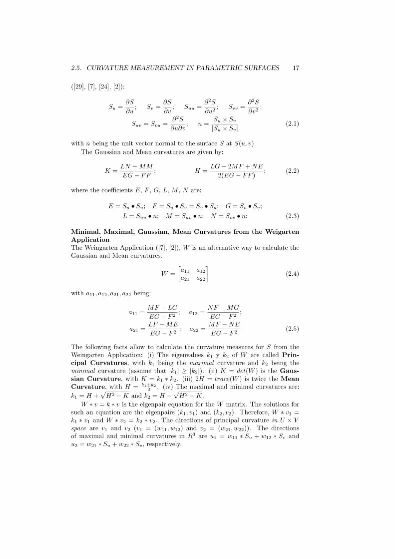
A parametric surface is a function S : R2 → R3, which we asume to be twicederivable in every point. The derivatives are named in the following manner
2.5. CURVATURE MEASUREMENT IN PARAMETRIC SURFACES 17
([29], [7], [24], [2]):
Su =∂S
∂u; Sv =
∂S
∂v; Suu =
∂2S
∂u2; Svv =
∂2S
∂v2;
Suv = Svu =∂2S
∂u∂v; n =
Su × Sv
|Su × Sv| (2.1)
with n being the unit vector normal to the surface S at S(u, v).The Gaussian and Mean curvatures are given by:
K =LN −MM
EG− FF; H =
LG− 2MF + NE
2(EG− FF ); (2.2)
where the coefficients E, F , G, L, M , N are:
E = Su • Su; F = Su • Sv = Sv • Su; G = Sv • Sv;L = Suu • n; M = Suv • n; N = Svv • n; (2.3)
Minimal, Maximal, Gaussian, Mean Curvatures from the WeigartenApplicationThe Weingarten Application ([7], [2]), W is an alternative way to calculate theGaussian and Mean curvatures.
W =[a11 a12
a21 a22
](2.4)
with a11, a12, a21, a22 being:
a11 =MF − LG
EG− F 2; a12 =
NF −MG
EG− F 2;
a21 =LF −ME
EG− F 2; a22 =
MF −NE
EG− F 2(2.5)
The following facts allow to calculate the curvature measures for S from theWeingarten Application: (i) The eigenvalues k1 y k2 of W are called Prin-cipal Curvatures, with k1 being the maximal curvature and k2 being theminimal curvature (assume that |k1| ≥ |k2|). (ii) K = det(W ) is the Gaus-sian Curvature, with K = k1 ∗ k2. (iii) 2H = trace(W ) is twice the MeanCurvature, with H = k1+k2
2 . (iv) The maximal and minimal curvatures are:k1 = H +
√H2 −K and k2 = H −√H2 −K.
W ∗ v = k ∗ v is the eigenpair equation for the W matrix. The solutions forsuch an equation are the eigenpairs (k1, v1) and (k2, v2). Therefore, W ∗ v1 =k1 ∗ v1 and W ∗ v2 = k2 ∗ v2. The directions of principal curvature in U × Vspace are v1 and v2 (v1 = (w11, w12) and v2 = (w21, w22)). The directionsof maximal and minimal curvatures in R3 are u1 = w11 ∗ Su + w12 ∗ Sv andu2 = w21 ∗ Su + w22 ∗ Sv, respectively.
18 CHAPTER 2. SURFACE TRIANGULATION
2.6 Methodology
2.6.1 Calculation of F−1
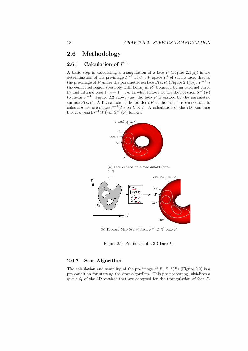
A basic step in calculating a triangulation of a face F (Figure 2.1(a)) is thedetermination of the pre-image F−1 in U × V space R2 of such a face, that is,the pre-image of F under the parametric surface S(u, v) (Figure 2.1(b)). F−1 isthe connected region (possibly with holes) in R2 bounded by an external curveΓ0 and internal ones Γi, i = 1, ..., n. In what follows we use the notation S−1(F )to mean F−1. Figure 2.2 shows that the face F is carried by the parametricsurface S(u, v). A PL sample of the border ∂F of the face F is carried out tocalculate the pre-image S−1(F ) on U × V . A calculation of the 2D boundingbox minmax(S−1(F )) of S−1(F ) follows.
(a) Face defined on a 2-Manifold (don-nut)
(b) Forward Map S(u, v) from F−1 ⊂ R2 onto F
Figure 2.1: Pre-image of a 3D Face F .
2.6.2 Star Algorithm
The calculation and sampling of the pre-image of F , S−1(F ) (Figure 2.2) is apre-condition for starting the Star algortihm. This pre-processing initializes aqueue Q of the 3D vertices that are accepted for the triangulation of face F .

2.6. METHODOLOGY 19
These initially determined vertices are the isometric sampling of the loops Li
forming the boundary of F .As the Star algorithm proceeds, a vertex p ∈ Q is extracted from Q. A star
is calculated around p (Figure 2.3(a)), lying on the plane Π[p, n] tangent to S atp with normal n (Equation 2.5). The star has radius r(H), and six (6) vertices.The radius r(H) of the star is inversely proportional to the mean curvature Hof S at p (Figure 2.3(a)). A number of vertices of the star are rejected if they(their projection on S) fall outside F . Additional vertices are rejected if theyare too close to the already accepted vertices inside F . The survivor verticesare projected on F and included in the queue Q. The algorithm for vertexcalculation stops when Q is empty.
After the vertex set VT on the face F is determined, a modified DelaunayTriangulation with the points in VT proceeds, which is explained later.
Figure 2.2: The iso-distance sample of edges on F generate the triangulationinitial vertex set.
2.6.3 Sprinkle Algorithm
Figure 2.3(b) displays the fact that the creation of random points (u, v) insideF−1 is encouraged in neighborhoods in which the curvature H is high. Thisis done in this manner: (i) Create a point (u, v) with (u, v) being randomnumbers and (u, v) inside minmax(S−1(F )). (ii) Return to step (i) if (u, v)is outside F−1, (iii) Assess (u, v) against curvature as follows: define a smallradius r(H) if a local high curvature S(u, v) exists, and vice versa. (iv) Reject(u, v) and go back to (i) if the 3D ball B(S(u, v), r(H)) contains another vertexalready marked on the face F . (v) Accept (u, v) if the ball B(S(u, v), r(H))on F contains no other vertex already accepted and mark S(u, v) on F as anacceptable vertice for the future triangulation. Include S(u, v) in the vertex set

20 CHAPTER 2. SURFACE TRIANGULATION
(a) Star algorithm. Sampling distance as function of thecurvature
(b) Sprinkle algorithm. Sprinkle focus as a function of thecurvature
Figure 2.3: Comparison between Star and Sprinkle algorithms for generation oftriangulation vertices.
VT .One knows that the face F is already sufficienty sprinkled by vertices if a
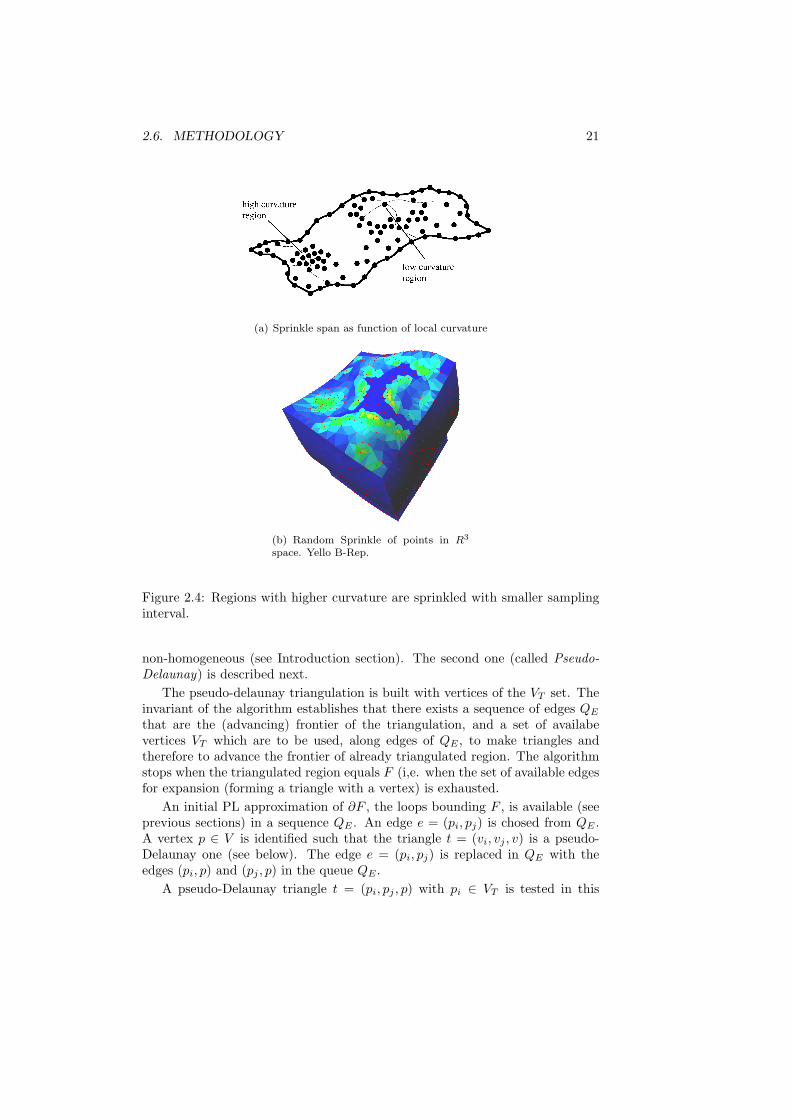
given number Nt of trials to mark vertices S(u, v) on F fails. The effect of suchheuristic is hinted in Figure 2.4(a). The result of the algorithm acting on a testB-rep is displayed in Figure 2.4(b). This B-Rep (called Yello) is specifically gen-erated to have faces with velocity in the u direction being dramatically diferentfrom the velocity in v direction, with which a grid generated in the U ×V spacewill produce a triangulation with folds and plies. In contrast, Figure 2.4(b)shows excellent aspect ratio (nearly equilateral) triangles.
A modified Delaunay Triangulation is calculated with the points in VT . Re-sults are shown in Figure 2.4(b).
2.6.4 A Pseudo - Delaunay Triangulation
To generate the connectivity information of the set of discretized points twoapproaches were used. The first one is to calculate a triangulation in parametricspace (using [35]). This approach does not produce satisfactory results wheneverthe warping of the U × V space with respect to the R3 euclidean distance is
2.6. METHODOLOGY 21
(a) Sprinkle span as function of local curvature
(b) Random Sprinkle of points in R3
space. Yello B-Rep.
Figure 2.4: Regions with higher curvature are sprinkled with smaller samplinginterval.
non-homogeneous (see Introduction section). The second one (called Pseudo-Delaunay) is described next.
The pseudo-delaunay triangulation is built with vertices of the VT set. Theinvariant of the algorithm establishes that there exists a sequence of edges QE
that are the (advancing) frontier of the triangulation, and a set of availabevertices VT which are to be used, along edges of QE , to make triangles andtherefore to advance the frontier of already triangulated region. The algorithmstops when the triangulated region equals F (i,e. when the set of available edgesfor expansion (forming a triangle with a vertex) is exhausted.
An initial PL approximation of ∂F , the loops bounding F , is available (seeprevious sections) in a sequence QE . An edge e = (pi, pj) is chosed from QE .A vertex p ∈ V is identified such that the triangle t = (vi, vj , v) is a pseudo-Delaunay one (see below). The edge e = (pi, pj) is replaced in QE with theedges (pi, p) and (pj , p) in the queue QE .
A pseudo-Delaunay triangle t = (pi, pj , p) with pi ∈ VT is tested in this
22 CHAPTER 2. SURFACE TRIANGULATION
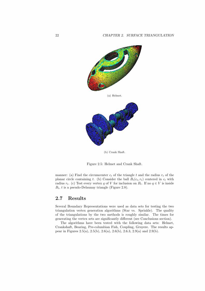
(a) Helmet.
(b) Crank Shaft.
Figure 2.5: Helmet and Crank Shaft.
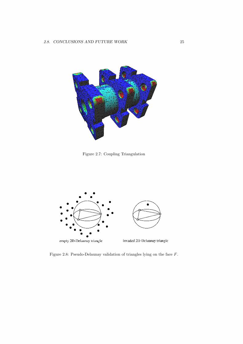
manner: (a) Find the circumcenter ct of the triangle t and the radius rt of theplanar circle containing t. (b) Consider the ball Bt(ct, rt) centered in ct withradius rt. (c) Test every vertex q of V for inclusion on Bt. If no q ∈ V is insideBt, t is a pseudo-Delaunay triangle (Figure 2.8).
2.7 Results
Several Boundary Representations were used as data sets for testing the twotriangulation vertex generation algorithms (Star vs. Sprinkle). The qualityof the triangulations by the two methods is roughly similar. The times forgenerating the vertex sets are significantly different (see Conclusions section).
The algorithms have been tested with the following data sets: Helmet,Crankshaft, Bearing, Pre-columbian Fish, Coupling, Gruyere. The results ap-pear in Figures 2.5(a), 2.5(b), 2.6(a), 2.6(b), 2.6.3, 2.9(a) and 2.9(b).
2.8. CONCLUSIONS AND FUTURE WORK 23
2.8 Conclusions and Future Work
The Star algorithm produces slightly better triangles than the Sprinkle algo-rithm. This advantage is to be expected, since the Star algorithm, by definition,creates on the tangent plane Π[n, p] a regular hexagon (i.e. 6 equilateral trian-gles) incident to the vertex p to expand, and projects them onto the F surface.In contrast, the Sprinkle algorithm is considerably more efficient for generatingthe vertex point set than the Star algorithm. The execution times are displayedin the following figures: Helmet, 2.10(a), Aphrodite data Set. 2.10(b) and Hand2.10(c). The statistics presented are concentrated in the generation of the vertexset, because the algorithm (pseudo-Delaunay) for the connection of the vertexset is common.
Future work is needed in the aspects of the numerical assessment of thegoodness of the triangle set, specifically in the application of Finite ElementAnalysis.

24 CHAPTER 2. SURFACE TRIANGULATION
(a) Bearing.
(b) Pre-columbian Fish.
Figure 2.6: Bearing and Pre-columbian Fish.
2.8. CONCLUSIONS AND FUTURE WORK 25
Figure 2.7: Coupling Triangulation
Figure 2.8: Pseudo-Delaunay validation of triangles lying on the face F .

26 CHAPTER 2. SURFACE TRIANGULATION
(a) Gruyere B-Rep triangulated with the Star Algo-rithm
(b) Gruyere B-Rep triangulated with the Sprinke Algo-rithm
Figure 2.9: Triangulations of Gruyere Boundary Representation

2.8. CONCLUSIONS AND FUTURE WORK 27
(a) Helmet data set.
(b) Aphrodite data Set.
(c) Hand data set.
Figure 2.10: Comparisson between Star and Sprinkle algorithms for generationtimes for triangulation vertices.

28 CHAPTER 2. SURFACE TRIANGULATION

Chapter 3
Adaptative cubical grid forisosurface extraction
3.1 Context
A project to device a method for the generation of real-time triangular tessel-lation of implicit surfaces was developed at VICOMTech Institute. The resultof this method generates a triangular tessellation of implicit surfaces whichcan be displayed in commodity computers in real time. This work has beenfounded by EAFIT University, the Colombian Council of Research and Tech-nology (COLCIENCIAS) and The Spanish Administration agency CDTI, underproject CENIT-VISION 2007-1007, VICOMTech Institute.
John Congote, research assistant under my direction in the CAD CAM CAELaboratory, was able to program the application of the devised methods. Forsuch a purpose, theoretical contributions were needed, which appear in:
• Adaptative Cubical Grid For Isosurface Extraction. John Congote, AitorMoreno, Inigo Barandiaran, Javier Barandiaran, Oscar E. Ruiz. 4th In-ternational Conference on Computer Graphics Theory and ApplicationsGRAPP-2009. ISBN 978-989-8111-67-8, pp 21-26. Feb 5-8, 2009. Lisbon,Portugal.
Authors
• John Congote1,2
• Aitor Moreno2
• Inigo Barandiaran2
• Javier Barandiaran2
• Oscar E. Ruiz.1
29
30 CHAPTER 3. ADAPTATIVE CUBICAL GRID
1. CAD CAM CAE Laboratory, EAFIT University Colombia
2. VICOMTech Institute, Spain
As co-authors of such publications, we give our permission for this materialto appear in this document. We are ready to provide any additional informationon the subject, as needed.
————————————Prof. Oscar E. [email protected] CAD CAM CAE LaboratoryEAFIT University, Medellin, COLOMBIA

3.2. ABSTRACT 31
3.2 Abstract
This work proposes a variation on the Marching Cubes algorithm, where thegoal is to represent implicit functions with higher resolution and better graphicalquality using the same grid size. The proposed algorithm displaces the verticesof the cubes iteratively until the stop condition is achieved. After each iter-ation, the difference between the implicit and the explicit representations arereduced, and when the algorithm finishes, the implicit surface representationusing the modified cubical grid is more detailed, as the results shall confirm.The proposed algorithm corrects some topological problems that may appear inthe discretisation process using the original grid.
3.3 Introduction
Surface representation from scalar functions is an active research topic in dif-ferent fields of computer graphics such as medical visualisation of MagneticResonance Imaging (MRI) and Computer Tomography (CT) [20]. This rep-resentation is also widely used as an intermediate step for several graphicalprocesses [27], such as mesh reconstruction from point clouds or track planning.The representation of a scalar function in 3D is known as implicit representationand is generated using continuous algebraic iso-surfaces, radial basis functions[8] [25], signed distance transform [12] or discrete voxelisations.
The implicit functions are frequently represented as a discrete cubical gridwhere each vertex has the value of the function. The Marching Cubes algo-rithm (MC) [22] takes the cubical grid to create an explicit representation ofthe implicit surface. The MC algorithm has been widely studied as has beendemonstrated by Newman [26]. The output of the MC algorithm is an explicitsurface represented as a set of connected triangles known as a polygonal repre-sentation. The original results of the MC algorithm presented several topologicalproblems as demonstrated by Chernyaev [9] and have already been solved byLewiner [21].
The MC algorithm divides the space in a regular cubical grid. For each cube,a triangular representation is calculated, which are then joined to obtain theexplicit representation of the surface. This procedure is highly parallel becauseeach cube can be processed separately without significant interdependencies.The resolution of the generated polygonal surface depends directly on the inputgrid size. In order to increase the resolution of the polygonal surface it isnecessary to increase the number of cubes in the grid, increasing the amount ofmemory required to store the values of the grid.
Alternative methods to the MC algorithm introduce the concept of generat-ing multi-resolution grids, creating nested sub-grids inside the original grid. Thespatial subdivision using octrees or recursive tetrahedral subdivision techniquesare also used in the optimisation of iso-surface representations. The commoncharacteristic of these types of methods is that they are based on adding morecells efficiently, to ensure a higher resolution in the final representation.
32 CHAPTER 3. ADAPTATIVE CUBICAL GRID
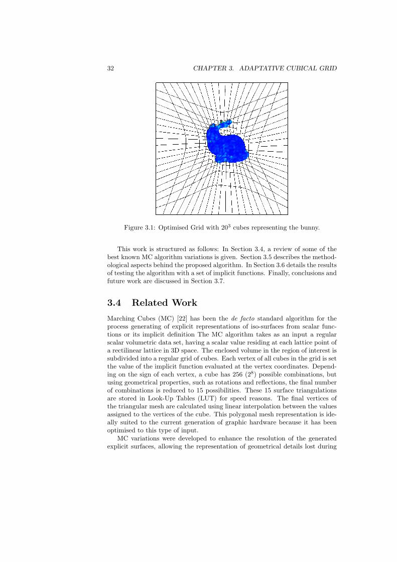
Figure 3.1: Optimised Grid with 203 cubes representing the bunny.
This work is structured as follows: In Section 3.4, a review of some of thebest known MC algorithm variations is given. Section 3.5 describes the method-ological aspects behind the proposed algorithm. In Section 3.6 details the resultsof testing the algorithm with a set of implicit functions. Finally, conclusions andfuture work are discussed in Section 3.7.
3.4 Related Work
Marching Cubes (MC) [22] has been the de facto standard algorithm for theprocess generating of explicit representations of iso-surfaces from scalar func-tions or its implicit definition The MC algorithm takes as an input a regularscalar volumetric data set, having a scalar value residing at each lattice point ofa rectilinear lattice in 3D space. The enclosed volume in the region of interest issubdivided into a regular grid of cubes. Each vertex of all cubes in the grid is setthe value of the implicit function evaluated at the vertex coordinates. Depend-ing on the sign of each vertex, a cube has 256 (28) possible combinations, butusing geometrical properties, such as rotations and reflections, the final numberof combinations is reduced to 15 possibilities. These 15 surface triangulationsare stored in Look-Up Tables (LUT) for speed reasons. The final vertices ofthe triangular mesh are calculated using linear interpolation between the valuesassigned to the vertices of the cube. This polygonal mesh representation is ide-ally suited to the current generation of graphic hardware because it has beenoptimised to this type of input.
MC variations were developed to enhance the resolution of the generatedexplicit surfaces, allowing the representation of geometrical details lost during

3.4. RELATED WORK 33
(a) Original Grid. The twospheres are displayed as a sin-gular object due to the poorresolution in the region
(b) Intermediate Grid. Bothspheres are displayed well,but are still joined
(c) Final Grid. The newresolution displays two wellshaped and separated sphereswith the same number ofcubes in the grid
Figure 3.2: 2D slides representing three different states in the evolution of thealgorithm of two nearby spheres
MC discretisation process. Weber [42] proposes a multi-grid method. Inside aninitial grid, a nested grid is created to add more resolution in that region. Thismethodology is suitable to be used recursively, adding more detail to conflictiveregions. In the final stage, the explicit surface is created by joining all thereconstructed polygonal surfaces.
It is necessary to generate a special polygonisation in the joints betweenthe grid and the sub-grids to avoid the apparition of cracks or artifacts. Thismethod has a higher memory demand to store the new values of the nested-grid.
An alternative method to refine selected region of interest is the octree sub-division [33]. This method generates an octree in the region of existence of thefunction, creating a polygonisation of each octree cell. One of the flaws of thismethod is the generation of cracks in the regions with different resolutions. Thisproblem is solve with the Dual Marching Cubes method [31] and implementedfor algebraic functions by Pavia [28]
The octree subdivision method produces edges with more than two vertices,which can be overcome by changing the methodology of the subdivision. Insteadof using cubes, tetrahedrons were used to subdivide the grid, without creatingnodes in the middle of the edges [17]. This method recursively subdivides thespace into tetrahedrons.
The previous methodologies increment the number of cells of the grid in orderto achieve more resolution in the regions of interest. Balmelli [5] presented analgorithm based on the movement of the grid to a defined region of interestusing a warping function. The result is a new grid with the same number of
34 CHAPTER 3. ADAPTATIVE CUBICAL GRID
cells, but with higher resolution in the desired region.Our method is also based on the displacement of the vertices of the grid,
obtaining dense distribution of vertices near to the iso-surface. (see Figure 3.2)
3.5 Methodology
The proposed algorithm is presented as a modification of the MC algorithm.The principal goal is the generation of more detailed approximations of thegiven implicit surfaces with the same grid resolution.
Applying a selective displacement to the vertices of the grid, the algorithmincreases the number of cells containing the iso-surface. In order to avoid self-intersections and to preserve the topological structure of the grid, the verticesare translated in the direction of the surface. The displacement to be appliedto each vertex is calculated iteratively until a stop condition is satisfied.
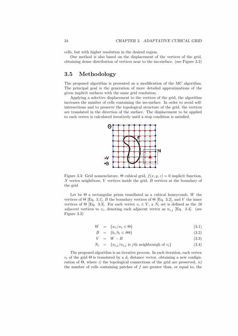
Figure 3.3: Grid nomenclature, Θ cubical grid, f(x, y, z) = 0 implicit function,N vertex neightboor, V vertices inside the grid, B vertices at the boundary ofthe grid
Let be Θ a rectangular prism tessellated as a cubical honeycomb, W thevertices of Θ [Eq. 3.1], B the boundary vertices of Θ [Eq. 3.2], and V the innervertices of Θ [Eq. 3.3]. For each vertex vi ∈ V , a Ni set is defined as the 26adjacent vertices to vi, denoting each adjacent vertex as ni,j [Eq. 3.4]. (seeFigure 3.3)
W = {wi/wi ∈ Θ} (3.1)B = {bi/bi ∈ δΘ} (3.2)V = W −B (3.3)Ni = {ni,j/ni,j is j th neighbourgh of vi} (3.4)
The proposed algorithm is an iterative process. In each iteration, each vertexvi of the grid Θ is translated by a di distance vector, obtaining a new configu-ration of Θ, where i) the topological connections of the grid are preserved, ii)the number of cells containing patches of f are greater than, or equal to, the

3.5. METHODOLOGY 35
Figure 3.4: two consecutives iterations are show where the vertex v is movedbetween the iterations t = 0 and t = 1. The new configuration of the grid isshown as dotted lines.
previous value, and iii) the total displacement [Eq. 3.7] of the grid is lower andis used as the stop condition of the algorithm when it reach a value ∆(see Figure3.4).
The distance vector di is calculated as shown in [Eq. 3.6] and it can be seenas the resultant force of each neighbouring vertex scaled by the value of f atthe position of each vertex. In order to limit the maximum displacement of thevertices and to guarantee the topological order of Θ, the distance vector di isclamped in the interval expressed in [Eq. 3.5]
0 ≤ |di| ≤ MIN( |ni,j − vi|
2
)(3.5)
di =126
∑ni,j
ni,j − vi
1 + |f(ni,j) + f(vi)| (3.6)
∑vi
|di| ≥ ∆ (3.7)
The algorithm stops when the sum of the distances added to all the verticesin the previous iteration is less that a given threshold ∆ [Eq. 3.7] (see Algorithm1).

36 CHAPTER 3. ADAPTATIVE CUBICAL GRID
repeats := 0;foreach Vertex vi do
di := 126
∑ni,j
ni,j−vi
1+|f(ni,j)+f(vi)| ;
mindist := MIN(|ni,j−vi|
2
);
di := diCLAMP(|di|, 0.0, mindist);vi := vi + di;s := s + |di|;
enduntil s ≥ ∆ ;
Algorithm 1: Vertex Displacement Pseudo-algorithm. |x| represents themagnitude of x, v represents the normalised vector of v
3.6 Results
Figure 3.5: Two balls in different positions with a scalar function as the distancetransform, representing the behaviour of the algorithm with different objects inthe space.
The proposed algorithm was tested with a set of implicit functions as distancetransforms (see Figure 3.5) and algebraic functions (see Figure 3.6(a)). Fordemonstration purposes, the number of cells has been chosen to be very low
3.6. RESULTS 37
GS31 MC. QLTY. AMC. QLTY. GS3
2
10 0.958555 - -20 0.369976 0.32257 1030 0.188298 0.186994 2040 0.129414 0.127588 3050 0.094878 0.092761 40
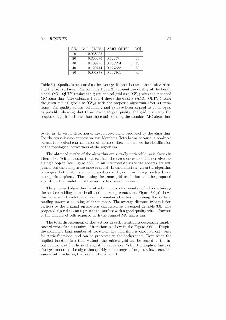
Table 3.1: Quality is measured as the average distance between the mesh verticesand the real surfaces. The columns 1 and 2 represent the quality of the bunnymodel (MC. QLTY.) using the given cubical grid size (GS1) with the standardMC algorithm. The columns 3 and 4 shows the quality (AMC. QLTY.) usingthe given cubical grid size (GS2) with the proposed algorithm after 30 itera-tions. The quality values (columns 2 and 3) have been aligned to be as equalas possible, showing that to achieve a target quality, the grid size using theproposed algorithm is less than the required using the standard MC algorithm.
to aid in the visual detection of the improvements produced by the algorithm.For the visualisation process we use Marching Tetrahedra because it producescorrect topological representation of the iso-surface, and allows the identificationof the topological correctness of the algorithm.
The obtained results of the algorithm are visually noticeable, as is shown inFigure 3.6. Without using the algorithm, the two spheres model is perceived asa single object (see Figure 3.2). In an intermediate state the spheres are stilljoined, but their shapes are more rounded. In the final state, when the algorithmconverges, both spheres are separated correctly, each one being rendered as anear perfect sphere. Thus, using the same grid resolution and the proposedalgorithm, the resolution of the results has been increased.
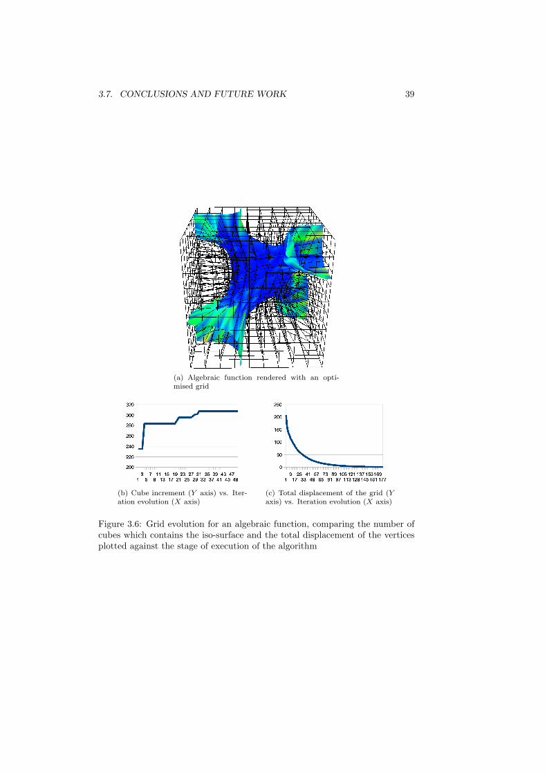
The proposed algorithm iteratively increases the number of cells containingthe surface, adding more detail to the new representation. Figure 3.6(b) showsthe incremental evolution of such a number of cubes containing the surface,tending toward a doubling of the number. The average distance triangulationvertices to the original surface was calculated as presented in table 3.6. Theproposed algorithm can represent the surface with a good quality with a fractionof the amount of cells required with the original MC algorithm.
The total displacement of the vertices in each iteration is decreasing rapidlytoward zero after a number of iterations as show in the Figure 3.6(c). Despitethe seemingly high number of iterations, the algorithm is executed only oncefor static functions, and can be processed in the background. Even when theimplicit function is a time variant, the cubical grid can be reused as the in-put cubical grid for the next algorithm execution. When the implicit functionchanges smoothly, the algorithm quickly re-converges after just a few iterationssignificantly reducing the computational effort.
38 CHAPTER 3. ADAPTATIVE CUBICAL GRID
3.7 Conclusions and Future Work
Our proposed iterative algorithm has shown significant advantages in the rep-resentation of distance transform functions. With the same grid size, it allows abetter resolution by displacing the vertices of the cube grids towards the surface,increasing the number of cells containing the surface.
The algorithm was tested with algebraic functions, representing distancetransform of the models. The generated scalar field has been selected to avoidthe creation of regions of false interest, which are for static images in whichthese regions are not used.
The number of iterations is directly related to the chosen value ∆ as it isthe stop condition. The algorithm will continuously displace the cube verticesuntil the accumulated displacement in a single iteration is less than ∆. In theresults, it can be seen that this accumulated distance converges quickly to thedesired value. This behaviour is very convenient to represent time varying scalarfunctions like 3D videos, where the function itself is continuously changing. Inthis context, the algorithm will iterate until a good representation of the surfaceis obtained. If the surface varies smoothly, the cube grid will be continuouslyand quickly readapted by running a few iterations of the presented algorithm.As the surface changes may be assumed to be small, the number of iterationsuntil a new final condition is achieved will be low. The obtained results will bea better real-time surface representation using a coarser cube grid.
3.7. CONCLUSIONS AND FUTURE WORK 39
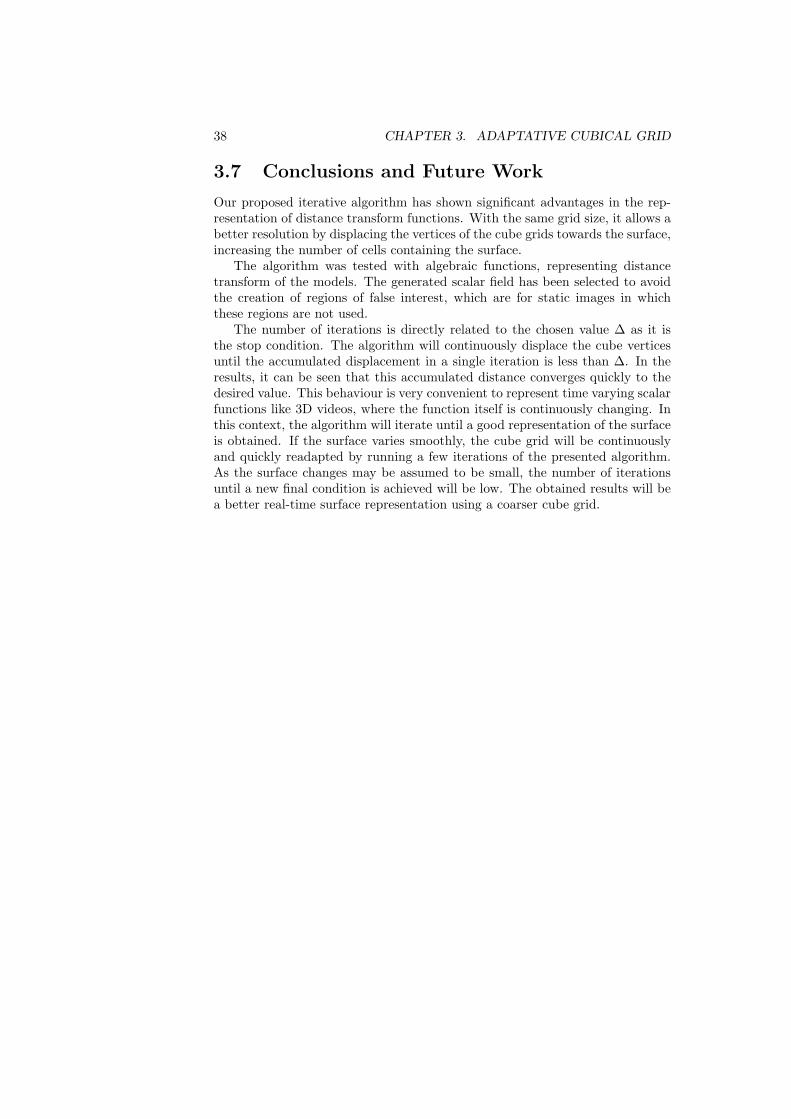
(a) Algebraic function rendered with an opti-mised grid
(b) Cube increment (Y axis) vs. Iter-ation evolution (X axis)
(c) Total displacement of the grid (Yaxis) vs. Iteration evolution (X axis)
Figure 3.6: Grid evolution for an algebraic function, comparing the number ofcubes which contains the iso-surface and the total displacement of the verticesplotted against the stage of execution of the algorithm

40 CHAPTER 3. ADAPTATIVE CUBICAL GRID

Chapter 4
Realtime dense stereomatching with dynamicprogramming in CUDA
4.1 Context
A project to device a method for the calculation of depth from to projectedimages in real-time was developed at VICOMTech Institute. The result ofthis method generates a dense depth map which indicates the distance from thecamera of the captured images in real-time using the graphic card for processing. This work has been founded by EAFIT University, the Colombian Council ofResearch and Technology (COLCIENCIAS) and The Spanish Administrationagency CDTI, under project CENIT-VISION 2007-1007, VICOMTech Institute.
John Congote, research assistant under my direction in the CAD CAM CAELaboratory, was able to program the application of the devised methods. Forsuch a purpose, theoretical contributions were needed, which appear in:
• Publication pending
Authors
• John Congote1,2
• Inigo Barandiaran2
• Javier Barandiaran2
• Oscar E. Ruiz.1
1. CAD CAM CAE Laboratory, EAFIT University Colombia
2. VICOMTech Institute, Spain
41

42 CHAPTER 4. REALTIME STEREO VISION
As co-authors of such publications, we give our permission for this materialto appear in this document. We are ready to provide any additional informationon the subject, as needed.
————————————Prof. Oscar E. [email protected] CAD CAM CAE LaboratoryEAFIT University, Medellin, COLOMBIA
4.2. ABSTRACT 43
4.2 Abstract
Real-time depth extraction from stereo images is an important process in com-puter vision. This paper proposes a new implementation of the dynamic pro-gramming algorithm to calculate dense depth maps using the CUDA archi-tecture achieving real-time performance with consumer graphics cards. Wecompare the running time of the algorithm against CPU implementations anddemonstrate the scalability property of the algorithm by testing it on differentgraphics cards.
4.3 Introduction
Dense depth map calculation is a common problem in computer vision. Wherein the image a depth distance is calculated for every pixel, generating a 3Dscene from the given image. The problem has been widely studied and diverseapproaches to solve the problem have been proposed [41] [18]. Furthermore, theproblem had been tracked since 2001 by Scharstein and Szeliski [32] who hadalso defined a taxonomy for stereo vision algorithms dividing them into local,global and scan-line, or semi-global methods. Depth map calculation is veryuseful in the area of robotics, 3D scene reconstruction, and in the emerging fieldof 3D television with technologies such as Philips WOWvx.
Real-time (RT) and near real-time algorithms to generate depth maps haveimproved substantially in recent years due to the following two factors. First,research in the field has developed new algorithms which reduce the complexityof algorithms and the increase in computational power required by the CPU,however these advances have been more dramatic with Graphic ProcessingUnit (GPU). New technologies such as Compute Unified Device Architecture(CUDA) opens a new promising field of work for these kinds of problems.Recently, much of the research has been carried out on the implementation ofdifferent depth estimation algorithms in GPU.
Local methods are more straightforward to implement using GPU. Thesemethods were measured and compared by Gong [15] and Tombari[39]. Alsoglobal methods were implemented in GPU, as shown by Gibson[14] and Yang[43].The highest quality results are achieved by using methods based on BeliefPropagation (BP)[18]. However, these methods are computationally intensive.Methodologies that strike a good balance between velocity and quality are al-gorithms that use a combination of a local method, dynamic programming anda post processing step, as demonstrated by Wang [40]. Our proposal is basedmainly on this work.
Dynamic Programming (DP) has been a difficult problem to solve in parallelarchitectures, as shown by Galil [13]. Some implementations of similar (DP)algorithms have been implemented in GPU, Manavski [23]. A useful practicalimplementation of the DP algorithm for depth map calculation has been at-tempted in the past by Gong [16] without achieving significant improvementsover comparative CPU implementations.
44 CHAPTER 4. REALTIME STEREO VISION
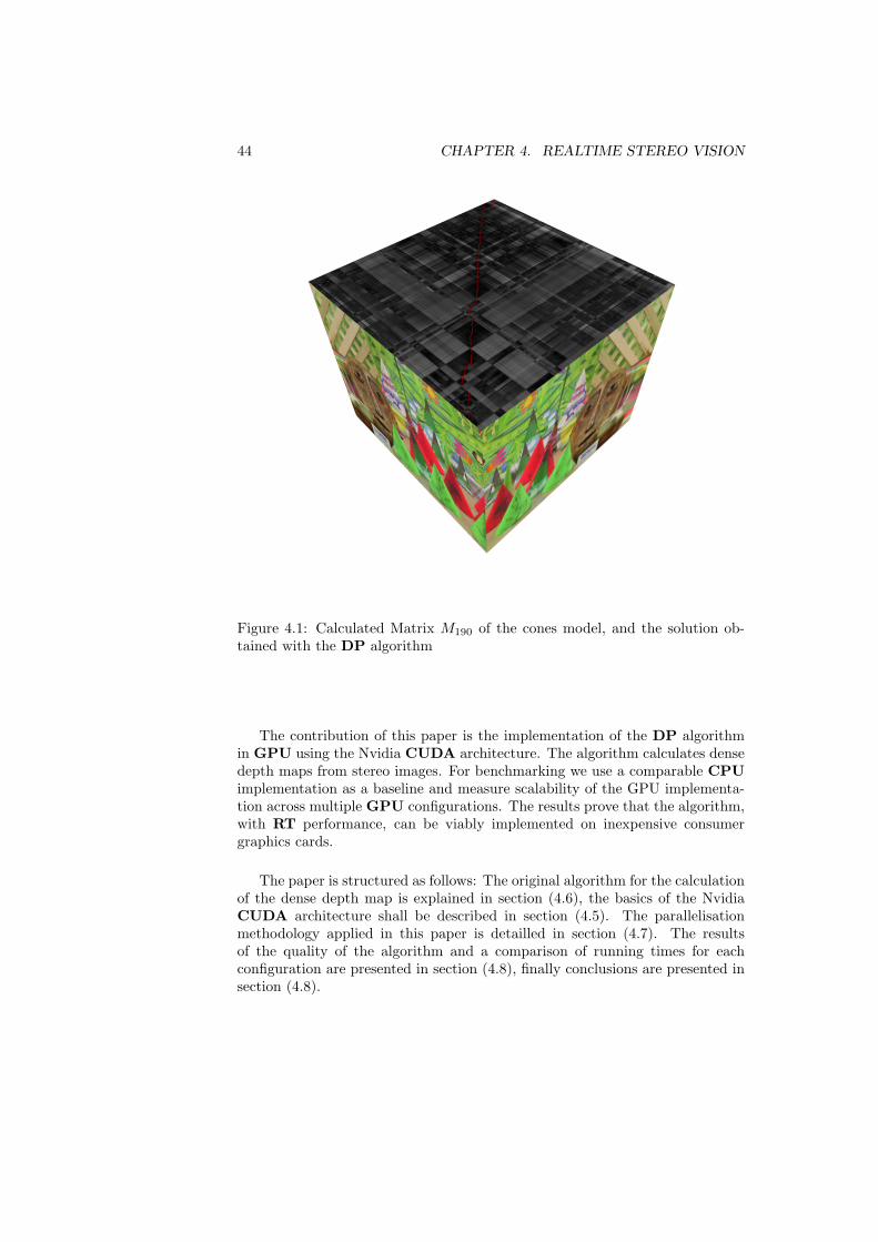
Figure 4.1: Calculated Matrix M190 of the cones model, and the solution ob-tained with the DP algorithm
The contribution of this paper is the implementation of the DP algorithmin GPU using the Nvidia CUDA architecture. The algorithm calculates densedepth maps from stereo images. For benchmarking we use a comparable CPUimplementation as a baseline and measure scalability of the GPU implementa-tion across multiple GPU configurations. The results prove that the algorithm,with RT performance, can be viably implemented on inexpensive consumergraphics cards.
The paper is structured as follows: The original algorithm for the calculationof the dense depth map is explained in section (4.6), the basics of the NvidiaCUDA architecture shall be described in section (4.5). The parallelisationmethodology applied in this paper is detailled in section (4.7). The resultsof the quality of the algorithm and a comparison of running times for eachconfiguration are presented in section (4.8), finally conclusions are presented insection (4.8).

4.4. GLOSARY 45
(a) Left image (b) Ground Truth
(c) Calculated Disparity
Figure 4.2: Depthmap calculation for teddy image of Middlebury stereo visiondata set. the calculated disparity was done using our algorithm and a medianfilter as a posprocessing step.
4.4 Glosary
DP: Dynamic Programming
RT: Real Time
CPU: Central Process Unit
GPU: Graphic Process Unit
CUDA: Computer Unified Device Architecture
BP: Belief propagation
GPGPU: General Purpose computation on GPU
SAD: Sum of Absolute Differences
RGB: Red-Green-Blue color space
46 CHAPTER 4. REALTIME STEREO VISION
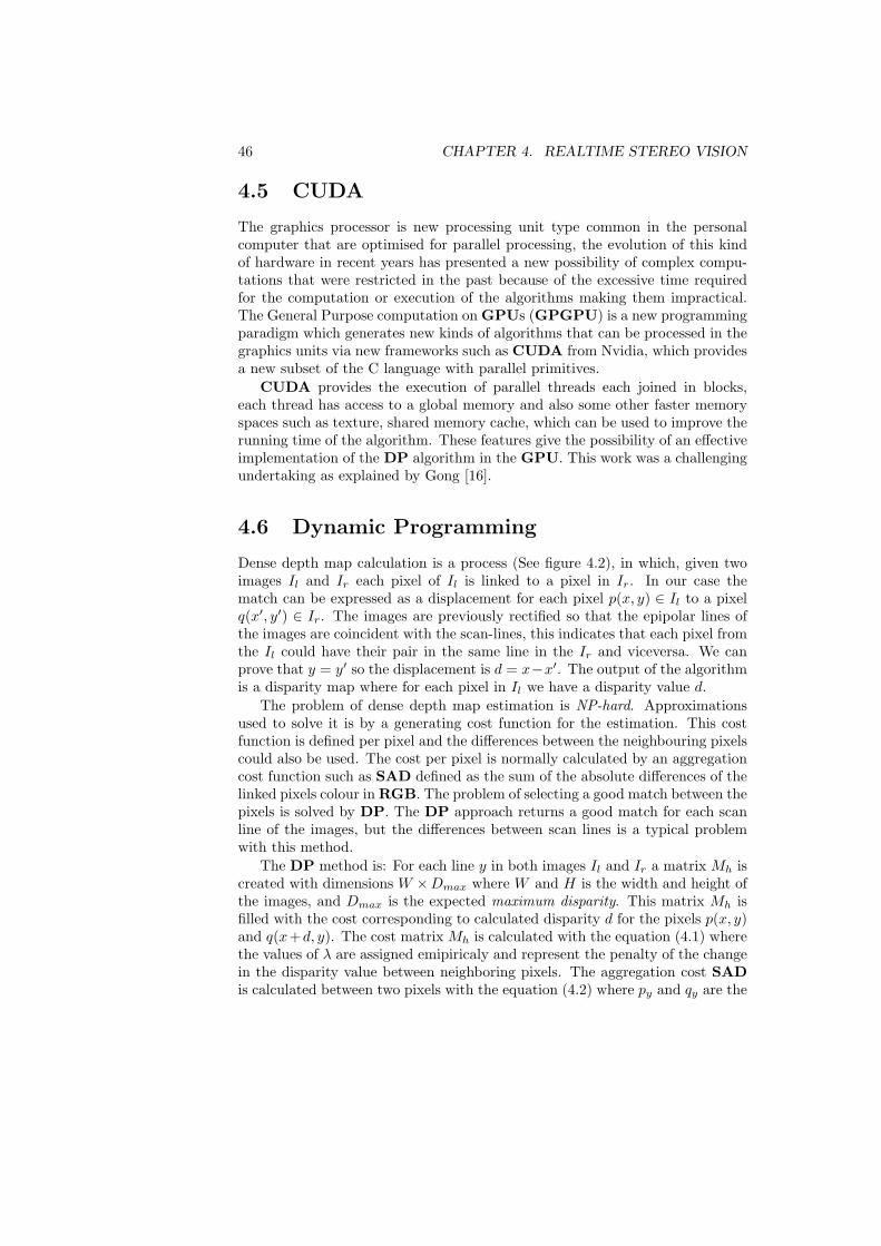
4.5 CUDA
The graphics processor is new processing unit type common in the personalcomputer that are optimised for parallel processing, the evolution of this kindof hardware in recent years has presented a new possibility of complex compu-tations that were restricted in the past because of the excessive time requiredfor the computation or execution of the algorithms making them impractical.The General Purpose computation on GPUs (GPGPU) is a new programmingparadigm which generates new kinds of algorithms that can be processed in thegraphics units via new frameworks such as CUDA from Nvidia, which providesa new subset of the C language with parallel primitives.
CUDA provides the execution of parallel threads each joined in blocks,each thread has access to a global memory and also some other faster memoryspaces such as texture, shared memory cache, which can be used to improve therunning time of the algorithm. These features give the possibility of an effectiveimplementation of the DP algorithm in the GPU. This work was a challengingundertaking as explained by Gong [16].
4.6 Dynamic Programming
Dense depth map calculation is a process (See figure 4.2), in which, given twoimages Il and Ir each pixel of Il is linked to a pixel in Ir. In our case thematch can be expressed as a displacement for each pixel p(x, y) ∈ Il to a pixelq(x′, y′) ∈ Ir. The images are previously rectified so that the epipolar lines ofthe images are coincident with the scan-lines, this indicates that each pixel fromthe Il could have their pair in the same line in the Ir and viceversa. We canprove that y = y′ so the displacement is d = x−x′. The output of the algorithmis a disparity map where for each pixel in Il we have a disparity value d.
The problem of dense depth map estimation is NP-hard. Approximationsused to solve it is by a generating cost function for the estimation. This costfunction is defined per pixel and the differences between the neighbouring pixelscould also be used. The cost per pixel is normally calculated by an aggregationcost function such as SAD defined as the sum of the absolute differences of thelinked pixels colour in RGB. The problem of selecting a good match between thepixels is solved by DP. The DP approach returns a good match for each scanline of the images, but the differences between scan lines is a typical problemwith this method.
The DP method is: For each line y in both images Il and Ir a matrix Mh iscreated with dimensions W ×Dmax where W and H is the width and height ofthe images, and Dmax is the expected maximum disparity. This matrix Mh isfilled with the cost corresponding to calculated disparity d for the pixels p(x, y)and q(x+d, y). The cost matrix Mh is calculated with the equation (4.1) wherethe values of λ are assigned emipiricaly and represent the penalty of the changein the disparity value between neighboring pixels. The aggregation cost SADis calculated between two pixels with the equation (4.2) where py and qy are the
4.7. PARALLEL DP 47
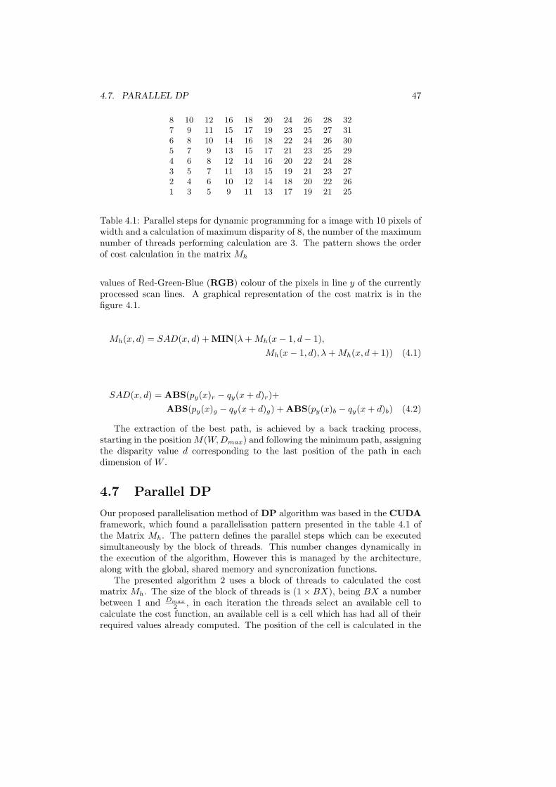
8 10 12 16 18 20 24 26 28 327 9 11 15 17 19 23 25 27 316 8 10 14 16 18 22 24 26 305 7 9 13 15 17 21 23 25 294 6 8 12 14 16 20 22 24 283 5 7 11 13 15 19 21 23 272 4 6 10 12 14 18 20 22 261 3 5 9 11 13 17 19 21 25
Table 4.1: Parallel steps for dynamic programming for a image with 10 pixels ofwidth and a calculation of maximum disparity of 8, the number of the maximumnumber of threads performing calculation are 3. The pattern shows the orderof cost calculation in the matrix Mh
values of Red-Green-Blue (RGB) colour of the pixels in line y of the currentlyprocessed scan lines. A graphical representation of the cost matrix is in thefigure 4.1.
Mh(x, d) = SAD(x, d) + MIN(λ + Mh(x− 1, d− 1),Mh(x− 1, d), λ + Mh(x, d + 1)) (4.1)
SAD(x, d) = ABS(py(x)r − qy(x + d)r)+ABS(py(x)g − qy(x + d)g) + ABS(py(x)b − qy(x + d)b) (4.2)
The extraction of the best path, is achieved by a back tracking process,starting in the position M(W,Dmax) and following the minimum path, assigningthe disparity value d corresponding to the last position of the path in eachdimension of W .
4.7 Parallel DP
Our proposed parallelisation method of DP algorithm was based in the CUDAframework, which found a parallelisation pattern presented in the table 4.1 ofthe Matrix Mh. The pattern defines the parallel steps which can be executedsimultaneously by the block of threads. This number changes dynamically inthe execution of the algorithm, However this is managed by the architecture,along with the global, shared memory and syncronization functions.
The presented algorithm 2 uses a block of threads to calculated the costmatrix Mh. The size of the block of threads is (1× BX), being BX a numberbetween 1 and Dmax
2 , in each iteration the threads select an available cell tocalculate the cost function, an available cell is a cell which has had all of theirrequired values already computed. The position of the cell is calculated in the
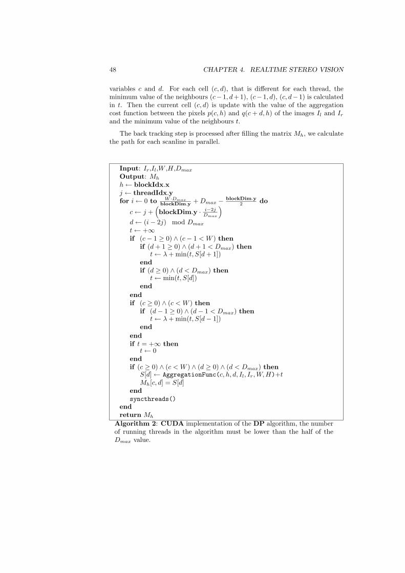
48 CHAPTER 4. REALTIME STEREO VISION
variables c and d. For each cell (c, d), that is different for each thread, theminimum value of the neighbours (c− 1, d+1), (c− 1, d), (c, d− 1) is calculatedin t. Then the current cell (c, d) is update with the value of the aggregationcost function between the pixels p(c, h) and q(c + d, h) of the images Il and Ir
and the minimum value of the neighbours t.
The back tracking step is processed after filling the matrix Mh, we calculatethe path for each scanline in parallel.
Input: Ir,Il,W ,H,Dmax
Output: Mh
h← blockIdx.xj ← threadIdx.yfor i← 0 to W ·Dmax
blockDim.y + Dmax − blockDim.y2 do
c← j +(blockDim.y · i−2j
Dmax
)
d← (i− 2j) mod Dmax
t← +∞if (c− 1 ≥ 0) ∧ (c− 1 < W ) then
if (d + 1 ≥ 0) ∧ (d + 1 < Dmax) thent← λ + min(t, S[d + 1])
endif (d ≥ 0) ∧ (d < Dmax) then
t← min(t, S[d])end
endif (c ≥ 0) ∧ (c < W ) then
if (d− 1 ≥ 0) ∧ (d− 1 < Dmax) thent← λ + min(t, S[d− 1])
endendif t = +∞ then
t← 0endif (c ≥ 0) ∧ (c < W ) ∧ (d ≥ 0) ∧ (d < Dmax) then
S[d]← AggregationFunc(c, h, d, Il, Ir,W,H)+tMh[c, d] = S[d]
endsyncthreads()
endreturn Mh
Algorithm 2: CUDA implementation of the DP algorithm, the numberof running threads in the algorithm must be lower than the half of theDmax value.
4.8. RESULTS 49
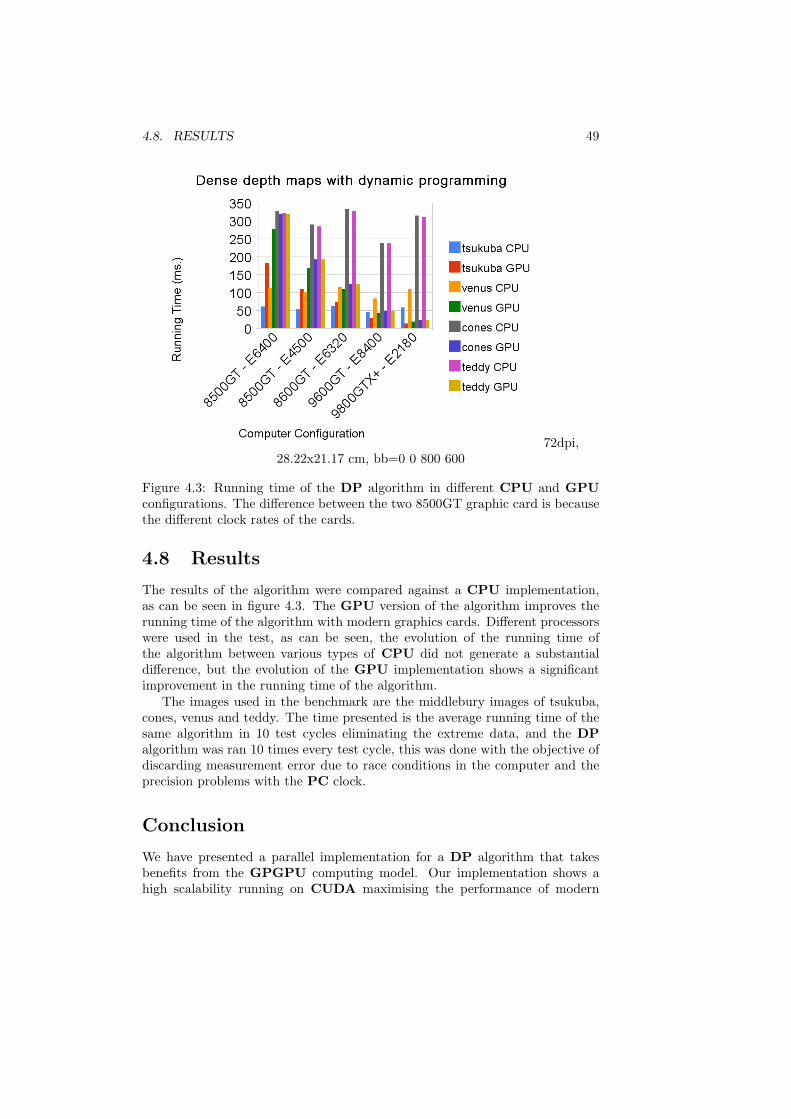
72dpi,28.22x21.17 cm, bb=0 0 800 600
Figure 4.3: Running time of the DP algorithm in different CPU and GPUconfigurations. The difference between the two 8500GT graphic card is becausethe different clock rates of the cards.
4.8 Results
The results of the algorithm were compared against a CPU implementation,as can be seen in figure 4.3. The GPU version of the algorithm improves therunning time of the algorithm with modern graphics cards. Different processorswere used in the test, as can be seen, the evolution of the running time ofthe algorithm between various types of CPU did not generate a substantialdifference, but the evolution of the GPU implementation shows a significantimprovement in the running time of the algorithm.
The images used in the benchmark are the middlebury images of tsukuba,cones, venus and teddy. The time presented is the average running time of thesame algorithm in 10 test cycles eliminating the extreme data, and the DPalgorithm was ran 10 times every test cycle, this was done with the objective ofdiscarding measurement error due to race conditions in the computer and theprecision problems with the PC clock.
Conclusion
We have presented a parallel implementation for a DP algorithm that takesbenefits from the GPGPU computing model. Our implementation shows ahigh scalability running on CUDA maximising the performance of modern

50 CHAPTER 4. REALTIME STEREO VISION
GPUs. These allows us to implement real-time stereo methods with increasingresolution and precision.
Chapter 5
Conclusion
Solutions for the four geometric problems have been presented in this work. Suchsolutions combine methodologies presented in different fields of computationalgeometry, computer graphics and computer vision. The successful applicationof the implemented solutions to real problems in the industries for which theywere built is one important contribution of this work.
The methodologies presented in this work represent and advance in the aca-demic field of the problems with the novel algorithms presented and also thepractical implementation in real environments with good results represent acomplete cycle of the I+D+I process.
Skills in literature reviewing, scientific rhetoric, paper writing and oral pre-sentation have been developed and strengthened throughout this work.
The valuable interaction with advisors, professors, and researchers at EAFITUniversity and Institutions abroad was essential in the successful developmentof this work. It was of particular importance the contact with other cultures,values and working environments.
51

52 CHAPTER 5. CONCLUSION

Bibliography
[1] Salim S. Abi-Ezzi and Srikanth Subramaniam. Fast dynamic tessellationof trimmed nurbs surfaced. Computer Graphics Forum, 13(”Issue 3”):107–126, 1994.
[2] Eduardo Aguirre. Geometria diferencial de curvas y superficies. Technicalreport, Departamento de Geometria y Topologia, Universidad ComplutenseMadrid, 2006. Apuntes de clase.
[3] Marco Attene, Bianca Falcidieno, Michela Spagnuolo, and Geoff Wyvill.A mapping-independent primitive for the triangulation of parametric sur-faces. Graph. Models, 65(5):260–273, 2003.
[4] Marco Attene, Bianca Falcidieno, Michela Spagnuolo, and Geoff Wyvill.A mapping-independent primitive for the triangulation of parametric sur-faces, 2003.
[5] Laurent Balmelli, Christopher J. Morris, Gabriel Taubin, and FaustoBernardini. Volume warping for adaptive isosurface extraction. In Proceed-ings of the conference on Visualization ’02, pages 467–474. IEEE ComputerSociety, 2002.
[6] M. Botsch and L. Kobbelt. A robust procedure to eliminate degener-ate faces from triangle meshes. In Vision, Modeling and Visualization(VMV01), Stuttgart, Germany, November 21 - 23, 2001, 2001.
[7] Manfredo Do Carmo. Differential geometry of curves and surfaces, pages1–168. Prentice Hall, 1976. ISBN: 0-13-212589-7.
[8] J. C. Carr, R. K. Beatson, J. B. Cherrie, T. J. Mitchell, W. R. Fright,B. C. McCallum, and T. R. Evans. Reconstruction and representation of 3dobjects with radial basis functions. In SIGGRAPH ’01: Proceedings of the28th annual conference on Computer graphics and interactive techniques,pages 67–76, New York, NY, USA, 2001. ACM.
[9] E. Chernyaev. Marching cubes 33: Construction of topologically correctisosurfaces. Technical report, Technical Report CERN CN 95-17, 1995.
53

54 BIBLIOGRAPHY
[10] Wonjoon Cho, Nicholas M. Patrikalakis, and Jaime Peraire. Approximatedevelopment of trimmed patches for surface tessellation. Computer AidedDesign, 30(14):1077–1087, December 1998.
[11] H. Date, S. Kanai, T. Kishinami, I. Nishigaki, and T. Dohi. High qual-ity and property controlled finite element mesh generation from triangularmeshes using multi-resolution technique. Journal of Computing and Infor-mation Science in Engineering, 5(4):266–276, 2005.
[12] Sarah F. Frisken, Sarah F. Frisken, Ronald N. Perry, Ronald N. Perry,Alyn P. Rockwood, Alyn P. Rockwood, Thouis R. Jones, and Thouis R.Jones. Adaptively sampled distance fields: A general representation ofshape for computer graphics. pages 249–254, 2000.
[13] Zvi Galil and Correspondence Kunsoo Park. Parallel dynamic program-ming. Technical report, Department of Computer Science Columbia Uni-versity, 1991.
[14] J. Gibson and O. Marques. Stereo depth with a unified architecture gpu.Computer Vision and Pattern Recognition Workshops, 2008. CVPRW ’08.IEEE Computer Society Conference on, pages 1–6, June 2008.
[15] Minglun Gong, Ruigang Yang, Liang Wang, and Mingwei Gong. A per-formance study on different cost aggregation approaches used in real-timestereo matching. Int. J. Comput. Vision, 75(2):283–296, 2007.
[16] Minglun Gong and Yee-Hong Yang. Near real-time reliable stereo matchingusing programmable graphics hardware. In CVPR ’05: Proceedings of the2005 IEEE Computer Society Conference on Computer Vision and PatternRecognition (CVPR’05) - Volume 1, pages 924–931, Washington, DC, USA,2005. IEEE Computer Society.
[17] Akinori Kimura, Yasufumi Takama, Yu Yamazoe, Satoshi Tanaka, andHiromi T. Tanaka. Parallel volume segmentation with tetrahedral adaptivegrid. ICPR, 02:281–286, 2004.
[18] A. Klaus, M. Sormann, and K. Karner. Segment-based stereo matchingusing belief propagation and a self-adapting dissimilarity measure. PatternRecognition, 2006. ICPR 2006. 18th International Conference on, 3:15–18,0-0 2006.
[19] R. Klein, A. Schilling, and W. Strasser. Illumination dependent refinementof multiresolution meshes. In Proceedings of Computer Graphics Interna-tional (CGI ’98), pages 680–687, Los Alamitos, CA, 1998. IEEE ComputerSociety Press.
[20] Premysl Krsek. Flow reduction marching cubes algorithm. In Proceedingsof ICCVG 2004, pages 100–106. Springer Verlag, 2005.

BIBLIOGRAPHY 55
[21] T. Lewiner, H. Lopes, A. Vieira, and G. Tavares. Efficient implementationof marching cubes’ cases with topological guarantees. Journal of GraphicsTools, 8(2):1–15, 2003.
[22] William E. Lorensen and Harvey E. Cline. Marching cubes: A high res-olution 3d surface construction algorithm. SIGGRAPH Comput. Graph.,21(4):169–169, 1987.
[23] Svetlin Manavski and Giorgio Valle. Cuda compatible gpu cards as effi-cient hardware accelerators for smith-waterman sequence alignment. BMCBioinformatics, 9(Suppl 2), 2008.
[24] Angel Montesdeoca. Apuntes de geometrıa diferencial de curvas y superfi-cies. Santa Cruz de Tenerife, 1996. ISBN: 84-8309-026-0.
[25] Bryan S. Morse, Terry S. Yoo, Penny Rheingans, David T. Chen, andK. R. Subramanian. Interpolating implicit surfaces from scattered surfacedata using compactly supported radial basis functions. In SIGGRAPH’05: ACM SIGGRAPH 2005 Courses, page 78, New York, NY, USA, 2005.ACM.
[26] Timothy S. Newman and Hong Yi. A survey of the marching cubes algo-rithm. Computers & Graphics, 30(5):854–879, October 2006.
[27] Carlos Cadavid Oscar E. Ruiz, Miguel Granados. Fea-driven geometricmodelling for meshless methods. In Virtual Concept 2005, pages 1–8, 2005.
[28] Afonso Paiva, Helio Lopes, Thomas Lewiner, and Luiz Henriquede Figueiredo. Robust adaptive meshes for implicit surfaces. SIBGRAPI,0:205–212, 2006.
[29] S. Palacios and O. Ruiz. Calculo de curvatura en superficies parametricas.A review of Literature on Curvature Measurement, December 2007.
[30] Giuseppe Patane, Michela Spagnuolo, and Bianca Falcidieno. Para-graph:Graph-based parameterization of triangle meshes with arbitrary genus.Computer Graphics Forum, 23(4):783–797, 2004.
[31] Scott Schaefer and Joe Warren. Dual marching cubes: Primal contouringof dual grids. In PG ’04: Proceedings of the Computer Graphics and Ap-plications, 12th Pacific Conference, pages 70–76, Washington, DC, USA,2004. IEEE Computer Society.
[32] Daniel Scharstein and Richard Szeliski. A taxonomy and evaluation ofdense two-frame stereo correspondence algorithms. International Journalof Computer Vision, 47:7–42, 2002.
[33] Raj Shekhar, Elias Fayyad, Roni Yagel, and J. Fredrick Cornhill. Octree-based decimation of marching cubes surfaces. In VIS ’96: Proceedings ofthe 7th conference on Visualization ’96, pages 335–ff., Los Alamitos, CA,USA, 1996. IEEE Computer Society Press.
56 BIBLIOGRAPHY
[34] J. Shewchuk. Delaunay refinement algorithms for triangular mesh gener-ation. Computational Geometry: Theory and Applications, 22(1–3):86–95,2002. citeseer.ist.psu.edu / shewchuk01delaunay.html.
[35] Jonathan Richard Shewchuk. Triangle: Engineering a 2D Quality MeshGenerator and Delaunay Triangulator. In Ming C. Lin and DineshManocha, editors, Applied Computational Geometry: Towards GeometricEngineering, volume 1148 of Lecture Notes in Computer Science, pages203–222. Springer-Verlag, May 1996. From the First ACM Workshop onApplied Computational Geometry.
[36] Jonathan Richard Shewchuk. General-dimensional constrained delaunayand constrained regular triangulations i: Combinatorial properties. Tech-nical report, Department of Electrical Engineering and Computer SciencesUniversity of California at Berkeley, Berkeley, CA 94720, December 2005.To appear in Discrete & Computational Geometry.
[37] C. Shu and P. Boulanger. Triangulating trimmed nurbs surfaces. In In-ternational Conference on Curves and Surfaces, Saint-Malo, France, pages381 – 388, May 2000.
[38] Wolfgang A. G. Stoger and Gerhard Kurka. Watertight tessellation ofb-rep nurbs cad-models using connectivity information. In Proceedings ofthe International Conference on Imaging Science, Systems and Technology,CISST ’03, June 23 - 26, 2003, Las Vegas, Nevada, USA, Volume 2. eds.Hamid R. Arabnia and Youngsong Mun. CSREA Press, 2003.
[39] F. Tombari, S. Mattoccia, L. Di Stefano, and E. Addimanda. Classifica-tion and evaluation of cost aggregation methods for stereo correspondence.Computer Vision and Pattern Recognition, 2008. CVPR 2008. IEEE Con-ference on, pages 1–8, June 2008.
[40] Liang Wang, Miao Liao, Minglun Gong, Ruigang Yang, and David Nis-ter. High-quality real-time stereo using adaptive cost aggregation anddynamic programming. In 3DPVT ’06: Proceedings of the Third Interna-tional Symposium on 3D Data Processing, Visualization, and Transmission(3DPVT’06), pages 798–805, Washington, DC, USA, 2006. IEEE Com-puter Society.
[41] Zeng-Fu Wang and Zhi-Gang Zheng. A region based stereo matching algo-rithm using cooperative optimization. Computer Vision and Pattern Recog-nition, 2008. CVPR 2008. IEEE Conference on, pages 1–8, June 2008.
[42] Gunther H. Weber, Oliver Kreylos, Terry J. Ligocki, John M. Shalf, BerndHamann, and Kenneth I. Joy. Extraction of crack-free isosurfaces fromadaptive mesh refinement data. In Data Visualization 2001 (Proceedingsof VisSym ’01), pages 25–34. Springer Verlag, 2001.

BIBLIOGRAPHY 57
[43] Q. Yang, L. Wang, R. Yang, S. Wang, M. Liao, and D. Nister. Real-timeglobal stereo matching using hierarchical belief propagation. In BMVC,pages 989–998. British Machine Vision Association, 2006.