Application of Wavelet Spectral Decomposition for …...Application of Wavelet Spectral Decomposition for Geological Interpretation of Seismic Data 233 represented with black color,

Journal of Geological Resource and Engineering 5 (2016) 231-241 doi:10.17265/2328-2193/2016.05.004

Application of Wavelet Spectral Decomposition for

Geological Interpretation of Seismic Data

Butorin A. V.

Expert Department of Geology and Exploration, LLC “Gazpromneft Science & Technology Centre” emb. rekiMoyki, 75-79,

Saint-Petersburg 190000, Russia

Abstract: Modern oil industry is on the way of complication of the geological structure of the deposits. This trend requires specialists to use the latest technologies to analyze available geological and geophysical information. The article describes a new algorithm—continuous wavelet transform in example of synthetic and real data. Key words: Seismic interpretation, spectral decomposition, RGB-blend, Achimov formation.

1. Introduction

At present, the development of hydrocarbon deposits

is conducted in conjunction with existing seismic data

monitoring, which allows predicting geological

environment within the target formation. The role of

the wave field increases in course of time due to the

need to involve in the development more and more

complex built deposits with variable non-uniform

internal structure, both laterally and vertically. This

need is related primarily to proportional decreasing of

relatively “simple” in terms of geology, structural

deposits, and transition to complex lithological traps.

Achimov layer of the Neocomian section in Western

Siberia is an example of this type of geological objects

in the Russian oil and gas industry, whose

accumulation is attached to the bottom of shelf terraces.

Deposits in Achimov complex are primarily controlled

by local areas of rapid sedimentation—accumulation

zones of sedimentary materialsbrought out from shelf

areas. Distribution collectors with this type of

sedimentation are irregular by area, making its forecast

in the interwell space impossible without 3D seismic

data [1].

Corresponding author: Butorin A. V., M.S. (geophysics),

postgraduate student, research fields: seismic interpretation, spectral analysis.

In addition to the areal irregularity such collectors

are distinctive also with relatively low thickness, which

imposes restrictions on usage of standard approaches in

seismic data analysis. The wave field has certain

resolution limit caused by band-limited frequency

spectrum of seismic signals. The maximum vertical

resolution is accepted to be 1/8-1/4 of the dominant

wavelength [2], which is 10-20 meters in average.

Based on these limitations, Achimov collectors are in

general objects stipulating the wave field interference,

i.e. the imposition of reflections from the top and

bottom of the reservoir. Interference nature of the wave

field is also a negative factor for seismic data

interpretation influencing the amplitude resolution.

A large number of limitations in the interpretation of

the wave field lead to increasing of dynamic

interpretation methods, which are an attempt to solve

the classic problem of geophysics—determining

environmental properties from the observed field

parameters such as time, amplitude, frequency and

phase, as well as their derivatives. Development of

algorithms for dynamic interpretation is directly

connected to the development of mathematics and

software for digital signal analysis.

Spectral representation of the wave field becomes

increasingly important in modern seismic exploration.

This approach to the dynamic parameters analysis is

D DAVID PUBLISHING

Application of Wavelet Spectral Decomposition for Geological Interpretation of Seismic Data

232

possible due to the development of spectral

decomposition technology, i.e. decomposition of

seismic data into frequency components [3]. Within

this article we will show the possibility to use this

technique for predicting reservoir properties both for

model and real data sets.

2. Materials and Methods

2.1 Theory of Spectral Decomposition

Frequency decomposition methods appeared in the

end of XX century. One of the first works in seismic

interpretation was an article [4], which discussed some

features of Fourier window transform application

(Gabor transformation) for geological interpretation.

Around the same time, the method of CWT

(continuous wavelet transform) appeared which later

used very widely in many different scientific and

practical fields.

Currently, there is insufficient knowledge regarding

the processes causing spectral anomalies.

Understanding of causes and patterns of observed

phenomena within application of the CWT method will

give an opportunity to use this algorithm more

competently and intelligently for the wave fields’

analysis.

The research described in this paper considers

frequency-dependent effects observed in the results of

CWT for synthetic wave field, calculated on the basis

of a given model. Observed regularities in change of

spectral parameters make it possible to determine basic

conditions and patterns of spectral anomalies, and also

to make some assumptionson optimal blending scheme

of results visualization for CWT method.

Spectral decomposition method allows us to

decompose the original wave field into separate

amplitude-frequency components. The described

methods are based on the assumption that local

studying of the wave field spectrum will provide more

information on internal structure of geological objects.

This algorithm was significantly developed since

appearance of the wavelet transform in the late XX

century, connected with works of Grossman and

Morlet. Wavelets are short waves with zero integral

value and the location on the independent variable axis

(time), able to shift along the axis and scaling. Due to

the short duration and different scale of wavelet,

decomposition allows us to explore local temporal

features of non-stationary processes occurring in time,

which is a significant advantage over the Fourier

transform, even in its window modification [5].

The presence of time shift allows us to scan studied

signal, i.e. explore it on different time levels. This

property of the wavelet transform makes it an

instrument for studying dynamic processes, i.e.

variable over time.

Scalability allows us to change the dominant

frequency, i.e. spectral composition of the wavelet.

Smaller scale factor values are used to obtain

high-frequency wavelets, larger values of the scaling

factor on the contrary lead to signal stretching, which

corresponds to the low-frequency wavelets.

Large number of wavelets can be used for CWT

method, but the most widely used is Ricker signal with

good localization in both time and frequency. Its major

positive point is the fact that it is similar with the real

seismic signals, which is positive for spectral

decomposition results of seismic data [6, 7].

2.2 Visualization of Spectral Decomposition Results

As a result of CWT spectral decomposition method,

the wave field can be decomposed into a series of cubes

describing the amplitude of the frequency harmonics

given. Further analysis of the spectral decomposition

results is to study amplitudes distribution of different

harmonics in area.

One of the most common methods of visualizing

CWT results is an RGB color blending. Three different

frequencies are applied to the input of the algorithm,

for example, vertical, horizontal or stratigraphic slices,

or cubes of frequency parameters. According to the

algorithm each data array is assigned a color code: red,

green or blue. The absence of harmonic amplitude


233

represented with black color, and its maximum

value—the highest saturation. Further, different color

channels are combined together so the resulting array

has three amplitude values corresponding to color

channel. Resulting color of the discrete is determined

by three-dimensional color cube, which describes all

colors combining red, green, and blue color channels

[8].

2.3 Interpretation of Color Combination Results on the

Basis of a Wedged Out Formation Model

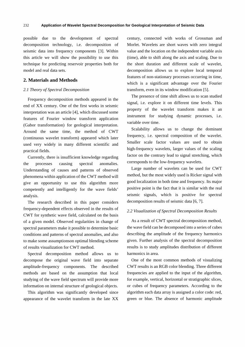
To study interpretation of RGB-mixing results we

performed a composition of a wedged out formation

synthetic model with variable acoustic impedance. The

model was composed with certain parameters as

follows: wedge thickness varies in one direction,

acoustic impedance varies in perpendicular direction,

and thus the impedance of the enclosing formation is

constant above and below the wedge. This model is a

good approximation of Achimov formation, where

sandstone reservoir intrudes into a relatively

homogeneous argillic matrix.

Ricker impulse signal with dominant frequency of

30 Hz was used for three-dimensional wave field

synthesis. In this case, the wave field simulation was

carried out considering vertical wave propagation

neglecting transient processes at the boundaries and

formation of harmonic waves. These assumptions

allow us to carry out a pure experiment in the “ideal”

field (Fig. 1).

The resulting synthetic wave field was applied to the

input of the CWT algorithm with Ricker signal. The

output produced cubes describing frequencies

amplitudes within the informative part of the spectrum.

For further analysis of the CWT results we studied

slices and RGB maps on various slices of the model

cube.

2.4 Studying Influence of Model Interference Effects on

Spectral Parameters

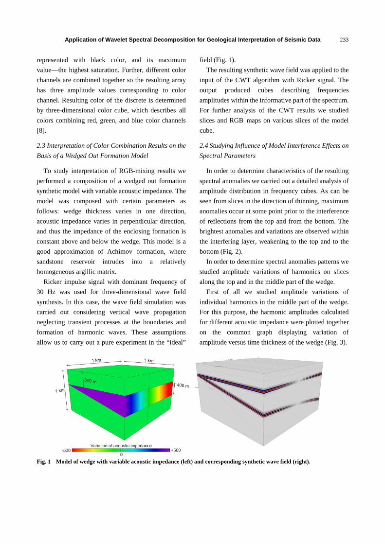
In order to determine characteristics of the resulting

spectral anomalies we carried out a detailed analysis of

amplitude distribution in frequency cubes. As can be

seen from slices in the direction of thinning, maximum

anomalies occur at some point prior to the interference

of reflections from the top and from the bottom. The

brightest anomalies and variations are observed within

the interfering layer, weakening to the top and to the

bottom (Fig. 2).

In order to determine spectral anomalies patterns we

studied amplitude variations of harmonics on slices

along the top and in the middle part of the wedge.

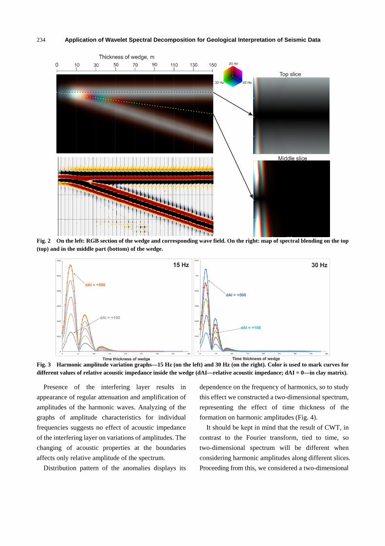
First of all we studied amplitude variations of

individual harmonics in the middle part of the wedge.

For this purpose, the harmonic amplitudes calculated

for different acoustic impedance were plotted together

on the common graph displaying variation of

amplitude versus time thickness of the wedge (Fig. 3).

Fig. 1 Model of wedge with variable acoustic impedance (left) and corresponding synthetic wave field (right).


234

Fig. 2 On the left: RGB section of the wedge and corresponding wave field. On the right: map of spectral blending on the top (top) and in the middle part (bottom) of the wedge.

Fig. 3 Harmonic amplitude variation graphs—15 Hz (on the left) and 30 Hz (on the right). Color is used to mark curves for different values of relative acoustic impedance inside the wedge (dAI—relative acoustic impedance; dAI = 0—in clay matrix).

Presence of the interfering layer results in

appearance of regular attenuation and amplification of

amplitudes of the harmonic waves. Analyzing of the

graphs of amplitude characteristics for individual

frequencies suggests no effect of acoustic impedance

of the interfering layer on variations of amplitudes. The

changing of acoustic properties at the boundaries

affects only relative amplitude of the spectrum.

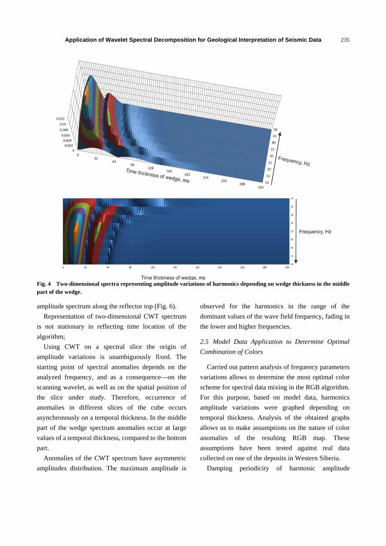
Distribution pattern of the anomalies displays its

dependence on the frequency of harmonics, so to study

this effect we constructed a two-dimensional spectrum,

representing the effect of time thickness of the

formation on harmonic amplitudes (Fig. 4).

It should be kept in mind that the result of CWT, in

contrast to the Fourier transform, tied to time, so

two-dimensional spectrum will be different when

considering harmonic amplitudes along different slices.

Proceeding from this, we considered a two-dimensional


235

Fig. 4 Two-dimensional spectra representing amplitude variations of harmonics depending on wedge thickness in the middle part of the wedge.

amplitude spectrum along the reflector top (Fig. 6).

Representation of two-dimensional CWT spectrum

is not stationary in reflecting time location of the

algorithm;

Using CWT on a spectral slice the origin of

amplitude variations is unambiguously fixed. The

starting point of spectral anomalies depends on the

analyzed frequency, and as a consequence—on the

scanning wavelet, as well as on the spatial position of

the slice under study. Therefore, occurrence of

anomalies in different slices of the cube occurs

asynchronously on a temporal thickness. In the middle

part of the wedge spectrum anomalies occur at large

values of a temporal thickness, compared to the bottom

part.

Anomalies of the CWT spectrum have asymmetric

amplitudes distribution. The maximum amplitude is

observed for the harmonics in the range of the

dominant values of the wave field frequency, fading in

the lower and higher frequencies.

2.5 Model Data Application to Determine Optimal

Combination of Colors

Carried out pattern analysis of frequency parameters

variations allows to determine the most optimal color

scheme for spectral data mixing in the RGB algorithm.

For this purpose, based on model data, harmonics

amplitude variations were graphed depending on

temporal thickness. Analysis of the obtained graphs

allows us to make assumptions on the nature of color

anomalies of the resulting RGB map. These

assumptions have been tested against real data

collected on one of the deposits in Western Siberia.

Damping periodicity of harmonic amplitude


236

parameters stipulates different results in color mixing.

Constructing an RGB map it is necessary to ensure

maximum color differentiation of objects, as well as

detailing of the resulting map.

Color differentiation is stipulated by combination of

extreme amplitude values of the graph. It should be

kept in mind that difference in the position of peaks

decreases with increasing frequency—difference in the

position of anomalies depending on the time thickness

of the layer varies sharply at low frequency for close

harmonics, difference in the amplitude parameters

levels at higher frequency.

Detailing of the resulting map is determined by the

maximum frequency of the harmonic wave used for the

RGB mixing. Higher frequencies carry more detailed

information, whereas lower frequencies are smooth

and reflect fewer details. Maximum frequency is

restricted by signal/noise ratio which varies depending

on the analyzed harmonic wave. Higher frequency is

characterized by a predominance of the noise

component due to natural damping processes and

seismic impulse spectrum, so its use is determined by

the quality of the wave field.

Analysis of damping distribution in

two-dimensional spectrum leads to the assumption that

increasing frequency above 40 Hz makes no sense,

since the behavior of anomalies remains approximately

the same.

The lower frequency during spectral analysis of real

seismic data is limited by the boundary of the

information availability. In most cases, the lower

frequency of the informative part of the spectrum can

be accepted at 10 Hz.

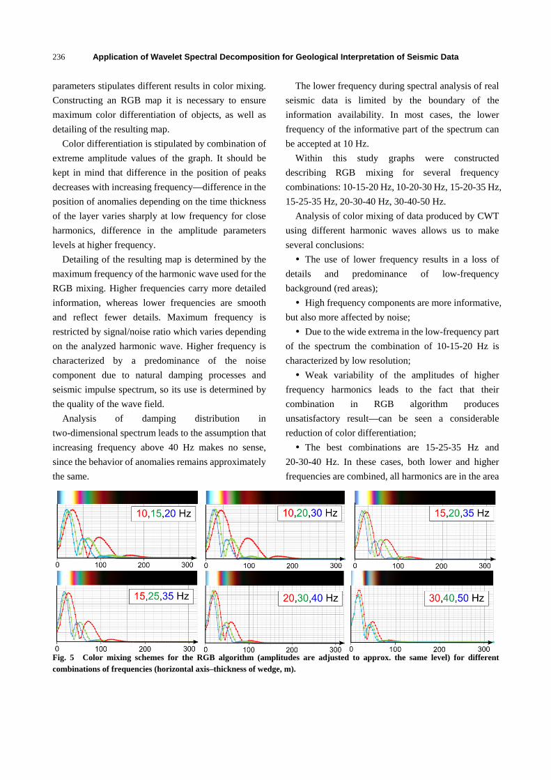
Within this study graphs were constructed

describing RGB mixing for several frequency

combinations: 10-15-20 Hz, 10-20-30 Hz, 15-20-35 Hz,

15-25-35 Hz, 20-30-40 Hz, 30-40-50 Hz.

Analysis of color mixing of data produced by CWT

using different harmonic waves allows us to make

several conclusions:

The use of lower frequency results in a loss of

details and predominance of low-frequency

background (red areas);

High frequency components are more informative,

but also more affected by noise;

Due to the wide extrema in the low-frequency part

of the spectrum the combination of 10-15-20 Hz is

characterized by low resolution;

Weak variability of the amplitudes of higher

frequency harmonics leads to the fact that their

combination in RGB algorithm produces

unsatisfactory result—can be seen a considerable

reduction of color differentiation;

The best combinations are 15-25-35 Hz and

20-30-40 Hz. In these cases, both lower and higher

frequencies are combined, all harmonics are in the area

Fig. 5 Color mixing schemes for the RGB algorithm (amplitudes are adjusted to approx. the same level) for different combinations of frequencies (horizontal axis–thickness of wedge, m).


237

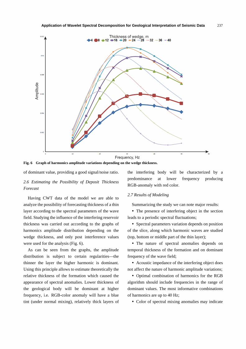
Fig. 6 Graph of harmonics amplitude variations depending on the wedge thickness.

of dominant value, providing a good signal/noise ratio.

2.6 Estimating the Possibility of Deposit Thickness

Forecast

Having CWT data of the model we are able to

analyze the possibility of forecasting thickness of a thin

layer according to the spectral parameters of the wave

field. Studying the influence of the interfering reservoir

thickness was carried out according to the graphs of

harmonics amplitude distribution depending on the

wedge thickness, and only post interference values

were used for the analysis (Fig. 6).

As can be seen from the graphs, the amplitude

distribution is subject to certain regularities—the

thinner the layer the higher harmonic is dominant.

Using this principle allows to estimate theoretically the

relative thickness of the formation which caused the

appearance of spectral anomalies. Lower thickness of

the geological body will be dominant at higher

frequency, i.e. RGB-color anomaly will have a blue

tint (under normal mixing), relatively thick layers of

the interfering body will be characterized by a

predominance at lower frequency producing

RGB-anomaly with red color.

2.7 Results of Modeling

Summarizing the study we can note major results:

The presence of interfering object in the section

leads to a periodic spectral fluctuations;

Spectral parameters variation depends on position

of the slice, along which harmonic waves are studied

(top, bottom or middle part of the thin layer);

The nature of spectral anomalies depends on

temporal thickness of the formation and on dominant

frequency of the wave field;

Acoustic impedance of the interfering object does

not affect the nature of harmonic amplitude variations;

Optimal combination of harmonics for the RGB

algorithm should include frequencies in the range of

dominant values. The most informative combinations

of harmonics are up to 40 Hz;

Color of spectral mixing anomalies may indicate


238

thickness distribution within geological bodies—thin

areas are characterized by the dominance of higher

frequency, relatively thick areas—mainly lower

frequency.

3. Results and Discussion

3.1 Practical Application

Obtained theoretical conclusions on CWT algorithm

were extrapolated to studying real formations in

Achimov formation attached to the development of

submarine fans in one of the deposits in Western

Siberia. Application of spectral decomposition allowed

increasing informational content of the results of

seismic data interpretation. Spectral data allow

determining cones geometry, and also the presence of

internal channels through which sediment distributed

inside the formation. This information is crucial for

development planning, as it allows to make an

assumption about internal anisotropy of properties

within the geologic body.

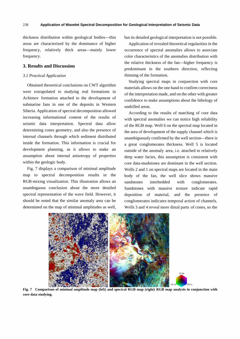
Fig. 7 displays a comparison of minimal amplitude

map to spectral decomposition results in the

RGB-mixing visualization. This illustration allows an

unambiguous conclusion about the more detailed

spectral representation of the wave field. However, it

should be noted that the similar anomaly area can be

determined on the map of minimal amplitudes as well,

but its detailed geological interpretation is not possible.

Application of revealed theoretical regularities in the

occurrence of spectral anomalies allows to associate

color characteristics of the anomalies distribution with

the relative thickness of the fan—higher frequency is

predominant in the southern direction, reflecting

thinning of the formation.

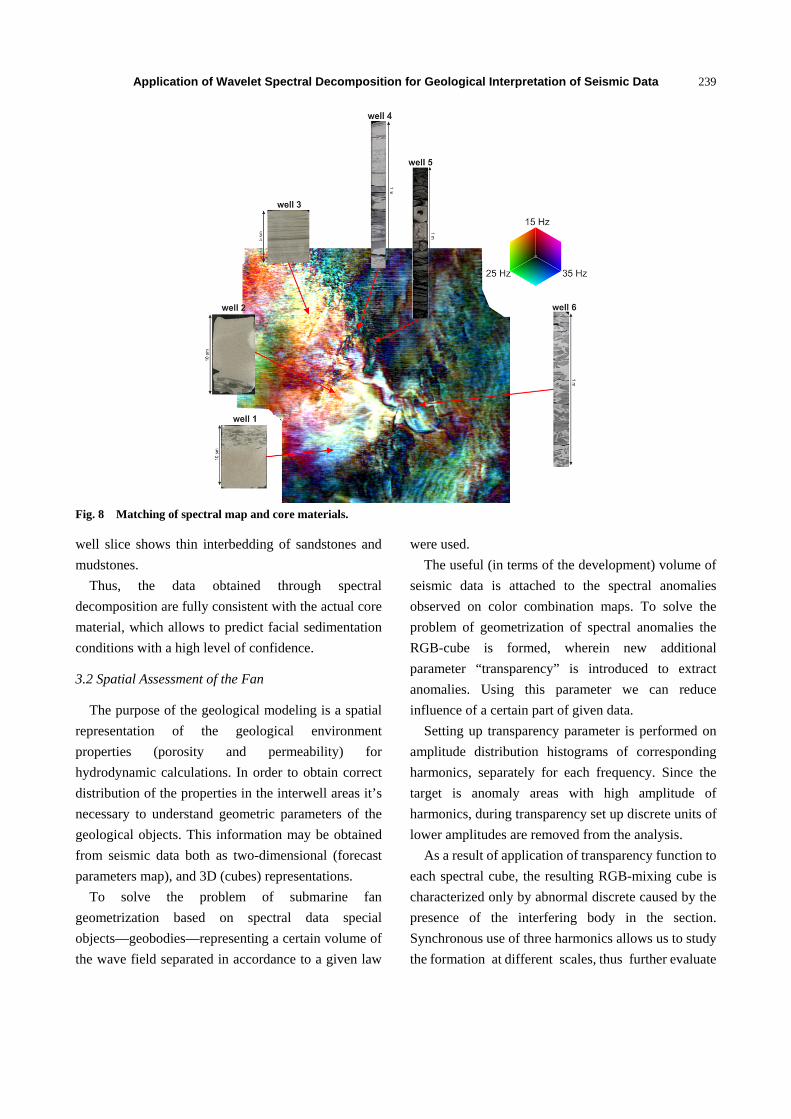
Studying spectral maps in conjunction with core

materials allows on the one hand to confirm correctness

of the interpretation made, and on the other with greater

confidence to make assumptions about the lithology of

undrilled areas.

According to the results of matching of core data

with spectral anomalies we can notice high reliability

of the RGB map. Well 6 on the spectral map located in

the area of development of the supply channel which is

unambiguously confirmed by the well section—there is

a great conglomerates thickness. Well 5 is located

outside of the anomaly area, i.e. attached to relatively

deep water facies, this assumption is consistent with

core data-mudstones are dominant in the well section.

Wells 2 and 1 on spectral maps are located in the main

body of the fan, the well slice shows massive

sandstones interbedded with conglomerates.

Sandstones with massive texture indicate rapid

deposition of material, and the presence of

conglomerates indicates temporal action of channels.

Wells 3 and 4 reveal more distal parts of cones, so the

Fig. 7 Comparison of minimal amplitude map (left) and spectral RGB map (right) RGB map analysis in conjunction with core data studying.


239

Fig. 8 Matching of spectral map and core materials.

well slice shows thin interbedding of sandstones and

mudstones.

Thus, the data obtained through spectral

decomposition are fully consistent with the actual core

material, which allows to predict facial sedimentation

conditions with a high level of confidence.

3.2 Spatial Assessment of the Fan

The purpose of the geological modeling is a spatial

representation of the geological environment

properties (porosity and permeability) for

hydrodynamic calculations. In order to obtain correct

distribution of the properties in the interwell areas it’s

necessary to understand geometric parameters of the

geological objects. This information may be obtained

from seismic data both as two-dimensional (forecast

parameters map), and 3D (cubes) representations.

To solve the problem of submarine fan

geometrization based on spectral data special

objects—geobodies—representing a certain volume of

the wave field separated in accordance to a given law

were used.

The useful (in terms of the development) volume of

seismic data is attached to the spectral anomalies

observed on color combination maps. To solve the

problem of geometrization of spectral anomalies the

RGB-cube is formed, wherein new additional

parameter “transparency” is introduced to extract

anomalies. Using this parameter we can reduce

influence of a certain part of given data.

Setting up transparency parameter is performed on

amplitude distribution histograms of corresponding

harmonics, separately for each frequency. Since the

target is anomaly areas with high amplitude of

harmonics, during transparency set up discrete units of

lower amplitudes are removed from the analysis.

As a result of application of transparency function to

each spectral cube, the resulting RGB-mixing cube is

characterized only by abnormal discrete caused by the

presence of the interfering body in the section.

Synchronous use of three harmonics allows us to study

the formation at different scales, thus further evaluate


240

Fig. 9 Algorithm of volume allocation of spectral anomalies. On the left—histogram amplitudes of harmonics with zeroed part, on the right—the result of applying a spatial filter.

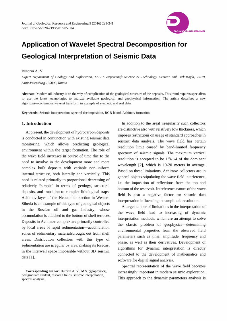
Fig. 10 On the left—horizontal well profile indicating intervals of oil, on the right—well position relative to the cone based on the spectral data.

geometry of the promising object, as can be seen from

the figure, the southern distal portion of the fan stands

out mainly at higher frequency harmonics (blue).

Discrete anomalies of RGB cube subsequently

digitized, i.e. are allocated as spot objects characterized

by three spatial coordinates.

This information allows us to construct a more

correct geological model, which describes spatial

distribution of geological bodies.

Detailing of the obtained spatial representation of

the submarine fan allows us to solve the problem of

geological modeling, and also to control paths of

horizontal wells. Fig. 10 shows the fan system

allocated according to the described method with paths

of horizontal wells imposed. An extended absence

interval of the collector can be observed on some part

of the horizontal well. Using obtained estimation of the

cone allows to determine that absence interval of the

collector corresponds to the outlet of the trunk from

productive body. Availability of corresponding


241

information prior to drilling will help to avoid such

situations in advance and to plan an optimal drilling

path.

4. Conclusion

This research was carried out to study

frequency-dependent effects observed on the wave

field in the presence of the interfering body. Basic

regularities were considered by the example of a

synthetic model of the wedge, which is a good

approximation of the collector model in Achimov

complex.

Studying of the synthetic model revealed that the

nature of spectral anomalies is not connected to

petrophysical properties of the formation, but in turn

reflects the level of interference on its top and bottom.

Constructed two-dimensional spectra of the model

allow us to determine a regular variation of harmonics

depending on the temporal thickness of the collector,

thereby determine the informative part of the spectrum.

The behavior of the amplitude parameters of harmonics

allows the assumption that the relative thickness of the

interfering object—dominant frequency increases with

reducing the thickness, which is reflected in the results

of the RGB-mixing.

Obtained theoretical conclusions are successfully

extrapolated to solve practical problems allocating

productive body associated with the development of

submarine fans. Detailing of the results allows highly

probable reconstructing of the internal structure of

geological bodies, which is a determining factor in

development drilling.

References

[1] Butorin, A. V. 2015. “The Internal Structure of Productive Clinoform Horizon by Seismic Data.” Geofizika 1: 10-8.

[2] Widess, M. B. 1973. “How Thin Is a Thin Bed?” Geophysics 38 (6): 1176-80.

[3] Castagna, J. 2006. “Comparison of Spectral Decomposition Methods.” First Break 24: 75-9.

[4] Partyka, G., Gridley, J., and Lopez, J. 1999. “Interpretational Application of Spectral Decomposition in Reservoir Characterization.” The Leading Edge 18 (3): 353-60.

[5] Dauberchies, I. 2001. Ten Lectures on Waveletes. Izhevsk: RHD, 464.

[6] Vityazev, V. V. 2001. Veyvletanalizvremennyhryadov [Wavelet Analysis of Time Series]. Saint-Petersburg: SPbSTU, 58.

[7] Yakovlev, A. N. 2003. Vvedenie v veyvlet-preobrazovanie [Introduction to Wavelet Transform]. Novosibirsk: NSTU, 104.

[8] Henderson. J., Purves. S. J., and Leppard C. 2007. “Automated Delineation of Geological Elements from 3D Seismic Data through Analysis of Multichannel, Volumetric Spectral Decomposition Data.” First Break 25: 87-93.

Documents

Application of Wavelet Spectral Decomposition for …...Application of Wavelet Spectral Decomposition for Geological Interpretation of Seismic Data 233 represented with black color,