water

Article

Application of Open Source Electronics forMeasurements of Surface Water Properties in anEstuary: A Case Study of River Jadro, Croatia

Vladimir Divic 1, Morena Galešic 1,*, Mariaines Di Dato 2, Marina Tavra 1 and Roko Andricevic 1,3

1 Faculty of Civil Engineering, Architecture and Geodesy, University of Split, 21000 Split, Croatia;vladimir.divic@gradst.hr (V.D.); mtavra@gradst.hr (M.T.); rokoand@gradst.hr (R.A.)

2 Helmholtz Centre for Environmental Research—UFZ, Department of Computational Hydrosystems,04318 Leipzig, Germany; mariaines.di-dato@ufz.de

3 Center of Excellence for Science and Technology-Integration of Mediterranean Region, University of Split,21000 Split, Croatia

* Correspondence: mgalesic@gradst.hr; Tel.: +385-95-564-0784

Received: 28 October 2019 ; Accepted: 7 January 2020 ; Published: 11 January 2020�����������������

Abstract: There are multiple factors affecting the behavior of water properties in an estuary, includingthe hydraulic properties of rivers and corresponding receiving water bodies, along with the potentialsolutes brought by rivers. Although there are various numerical models and analytical approaches tosolving particular or holistic problems in estuaries, measurements are inevitably required. In thisstudy, we developed an innovative low-cost probe based on the Arduino platform as an alternativeto more expensive measuring systems. Our device is designed to measure position, temperature,and electrical conductivity in multiple realizations, and it consists of a floating container equippedwith the following components: an Arduino Mega development board, a power managementmodule, an SD card logging module, a Bluetooth module, a temperature measuring module, a globalpositioning satellite (GPS) position module, and a newly developed module for measuring electricalconductivity (EC). We emphasize that all used tools are open-source and greatly supported by theworldwide community. We tested our probe during a field campaign conducted at the estuary ofRiver Jadro near Split (Croatia). Nine probes were released at the river mouth and their position,temperature, and EC were monitored and recorded during the experiment, which ended whenthe probes stopped, due to the river plume attenuation. The same experiment was repeated threetimes. All of the probes recorded consistent temperature data, while the EC data show more variablebehavior, due to the higher sensitivity of the corresponding sensor. This was expected as a part ofthe natural process in the estuary. The measured data were additionally used to parameterize ananalytical model for mean flow velocity and salinity as a proxy concentration. This showed a goodmatch between the experimental results and the theoretical framework. This work, although focusedon water surface applications in the near field zone of an estuary, should be considered as a promisingstep toward the development of innovative and affordable measurement devices.

Keywords: estuaries; field measurements; Arduino; low-cost measurement system; salinityimportance; conservative solute proxy.

1. Introduction

Estuaries are dynamic ecosystems that experience constant environmental changes due to theirnature of being a transition zone among land, river, and sea. Historically, estuarine science has evenbeen considered as a “poor relation” between freshwater and marine science [1]. However, among allthe surface water resources, estuaries and coastal ecosystem represent one of the richest and the most

Water 2020, 12, 209; doi:10.3390/w12010209 www.mdpi.com/journal/water

Water 2020, 12, 209 2 of 29

threatened natural systems globally [2,3]. The importance of estuaries is reflected in the value theydeliver through their ecosystems, ranging from direct consumable benefits to indirect benefits thatsupport the local biome and geophysical processes [4–7].

In an attempt to protect and preserve estuarine values, environmental directives and guidelineshave incorporated estuaries within multiple regulations. For instance, in the United States, estuariesare covered by the National Estuary Program within the Clean Water Act [8], while, in the EuropeanUnion (EU), they are well represented in the Water Framework Directive (WFD), the European BathingWater Directive (EUBWD), and the Marine Strategy Framework Directive (MSFD) [9–11], and arespecifically treated as transitional waters.

However, most of these programs have the same obstacle when it comes to implementation,and that is the scarcity of data, in particular, spatial data, which has already been covered bymultiple studies [12–15]. The INSPIRE (Infrastructure for Spatial Information in Europe) Directive [16]addresses this issue by acting as an umbrella platform covering the spatial data infrastructure forEU environmental policies and activities. In particular, Marine Spatial Data Infrastructure (MSDI)is focused on coastal areas [17] where it is closely related to both WFD and MSFD. Similar to otherMember States, Croatia has introduced MSDI into the national legislative framework within the fullyfunctional National Spatial Data Infrastructure (NSDI). Furthermore, a planning support concept wasapplied [18] and key stakeholders have identified priority data themes, but there are few data availableonline at this moment [19]. Consequently, MSDI development should follow monitoring efforts toenable better availability of spatial data and inter-operability.

The monitoring requirements issued by the above-mentioned regulations are pressing MemberStates and corresponding environmental agencies to assign a significant amount of resources to obtaindata on water properties. The goal is to continuously assess the ecological status of certain waterbodies and work on an improvement if needed [20]. When analyzing the concentration distributionsand dilution processes, which are intrinsically random, corresponding field experiments of repetitiousrealizations for dye release are quite expensive and tedious. In particular, Riddle and Lewis [21]studied the mixing process in coastal waters by collecting and analyzing tracer dye experiments in37 locations (among them, 25 were from the UK, five were from beaches in Malaysia and Singapore,and the last two were from France and China). Their datasets were composed of a total of 285 dyeexperiments recorded between 1968 and 1996. In addition, Rodriguez et al. [22] carried out a fieldexperiment at the Delta Ebro surf zone, in Spain, over 13–17 December 1993. Their experimental designcomprised simultaneous quantification of several parameters, such as incident waves, spatial velocity,and dispersion of five types of dyes. The process was repeated for eight cases. Later, Clarke et al. [23]quantified the dispersion coefficients in Santa Monica Bay by analyzing the statistics of 14 dye releasesfrom 1999 to 2000. Continuous research has also been done to predict some of the parameterswithout interfering in the environment itself, for instance in micro-tidal, river dominated estuaries inCroatia [24,25] with the focus on the distribution of potential conservative pollution brought to coastalwaters by rivers, or in a broader sense in New Zealand estuaries [26].

Among different water properties in estuaries, salinity is one of the most studied [27,28], both forits importance to the ecosystem (hydrodynamics and biome), and for its cost-effective measurement asopposed to, for instance, biological parameters. For instance, Wiseman et al. [29] analyzed the salinitytrend of two historical datasets from estuarine waters in south Louisiana (USA); their study showssignificant trends in mean salinity, salinity variance, and maximum salinity. Later, Bradley et al. [30]modeled the salinity decrease caused by a discharge reduction at Cooper River (South Carolina, USA),which occurred in 1985, thereby observing considerable changes in estuarine plant distribution. In arecent paper, Lorenz [31] reviewed the data on vertebrate fauna at Florida Bay (USA), finding astrong correlation between decrease in estuarine population and increase in salinity level. Similarrelationships between salinity concentration and estuarine ecosystems indicators were observedby Spalding and Hester [32] for coastal Louisiana (USA); by Rivera-Monroy et al. [33] at CiénagaGrande de Santa Marta–Pajarales Lagoon Complex (Colombia); and by Little et al. [34] in Southern

Water 2020, 12, 209 3 of 29

England (UK). Moreover, salinity may be used to determine multiple hydrological properties indirectly(e.g., coefficient of diffusion, velocity, and concentration statistics), as shown by several authors, such asVallino and C.S. Hopkinson [35] for Plum Island Sound estuary (Massachusetts, USA); Ho et al. [36]for the estuary of Hudson River in New York (USA); Gay and O’Donnell [37] for the Mid-Atlantic(USA); Xu et al. [38] for Chesapeake Bay (USA); Ref. [39] in the coastal zone of north-eastern Japan;and Andricevic and Galešic [40] for the River Žrnovnica in Split (Croatia). This approach has beenanalyzed [40,41], by measuring the salinity at different points in time with a commercial probe,the Sea-Bird’s SBE 37-SI MicroCAT. Depending on the final goal of the comparison between measuredand modeled data, different spatial configurations of the measured points were previously plannedand executed accordingly within four measurement campaigns on the River Žrnovnica [42].

We emphasize that measured salinity data were well aligned with the theoretical frameworkbased on the analytical model for solute concentration statistics. Results were good, but their qualitycould have been affected by the lack of temporal synchronization. That previous study was a keymotivation in developing the measurement system described in this manuscript, as it would have beenpreferable if the points were measured simultaneously at multiple positions. Since having multiplecommercial probes such as SBE 37-SI MicroCAT is rather expensive and sub-optimal, a lower-costconcept is proposed. Several previous studies have shown this kind of approach to be promising.For instance, a new multi-sensor buoy system was developed by enabling the remote monitoring ofmarine pressure, temperature, and atmospheric pressure [43]. Later, it was broadened to multiple otherparameters, such as chlorophyll a and Chromophoric Dissolved Organic Matter fluorescence [44].

However, such field measurements are often carried by means of costly probes, which mayhamper the quantity of available datasets. A possible way to reduce the cost of monitor devices iscollecting data by using Arduino-based [45] sonde. Arduino is a hardware and software companydevoted to designing and manufacturing open-source microcontrollers for digital devices, whichare specifically conceived to be user-friendly and easy to use. In a recent study, Lockridge et al. [46]developed an innovative low-cost Arduino based sonde able to measure data in coastal applications.Their paper describes both the manufacturing phase and the application test, which was comprised oftwo different conditions. During the first field measurement, six sondes were used as a free floatingLagrangian drifters and the data collected were position, velocity, and salinity; whereas during thesecond field measurement, the sondes collected data in a fixed position underwater for a long timeperiod. Their results show a good agreement of dataset with expected environmental conditions, thusbeing a reference for Arduino based sondes as a promising tool for environmental monitoring.

In this manuscript, we implemented a similar framework as the one previously addressedby Lockridge et al. [46]; however, the main distinctions are lower cost and higher flexibility dueto the custom made electrical conductivity (EC) sensor, as described in Section 2.3, although ourapproach requires a more complex calibration procedure (Section 2.4.2). Furthermore, while the systemdeveloped by Lockridge et al. [46] was introduced to have long-term applications and specific depths(defined by mooring positions), we were exclusively interested in surface water properties data inshort-term applications.

Our focus was to have multiple realizations in shorter time periods in order to obtain velocities,temperature, and salinity concentration statistics in the near field zone of an estuary. Our probes werenot supposed to be left without supervision, and the main focus was to enable better validation ofpreviously proposed analytical models by obtaining necessary parameters and testing the salinity as aproxy concentration. To obtain our goal, the probes were designed to float, to be easily deployable,light, and user-friendly. Furthermore, even though the Arduino system was used as the electronic basefor the probe, the process itself is organized quite differently than other commercial options, in orderto make it more cost-available, possibly even expendable, which is further explained in Section 2.3.It is important to emphasize that one may build such a probe with basic electronic tools. The cost ofcommercial probes is mainly due to sensors for electrical conductivity, which are often quite expensiveand operate as black-box solutions with limited user access to the internal setup. The great advantage

Water 2020, 12, 209 4 of 29

of developing our hand-crafted EC system dwells on its cost, i.e., less than 1/10 of an off-the-shelfversion, which allows technicians to manufacture probes in large quantities. However, a downside ofthe proposed system is a more complex calibration scheme, as explained in Section 2.4.2.

The capabilities and potentialities of the probes were tested in a field experiment conductedat River Jadro, near the city of Split, Croatia. In Section 2 we present the study area along with ashort description of field experiments. More importantly, the procedure of measurement systemdevelopment (Section 2.3) and data acquisition (Sections 2.4.1–2.4.3) are described. Specific focus isgiven to the calculation of both velocity and salinity data, which are needed for the additional andimproved validation of previous research [24,40–42]. Within Section 3.1, the obtained data are shown,while final applications for obtaining the parameters needed for further modeling are displayed inSection 3.2. In Section 3.3, we test and discuss the observed properties of the proposed measurementsystem, its limitations, and detected problems. Finally, we developed our conclusions on usability,achieved water properties data acquisition, and potential future applications and works (Section 4).

2. Materials and Methods

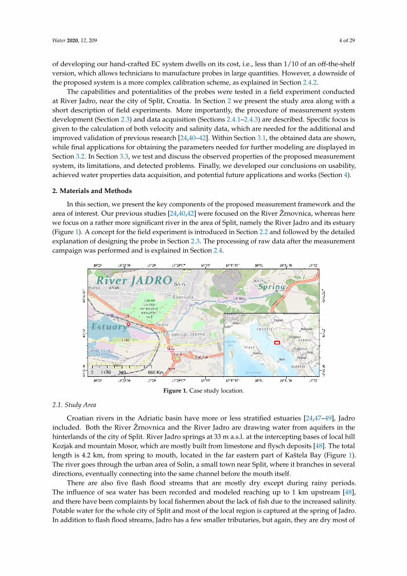
In this section, we present the key components of the proposed measurement framework and thearea of interest. Our previous studies [24,40,42] were focused on the River Žrnovnica, whereas herewe focus on a rather more significant river in the area of Split, namely the River Jadro and its estuary(Figure 1). A concept for the field experiment is introduced in Section 2.2 and followed by the detailedexplanation of designing the probe in Section 2.3. The processing of raw data after the measurementcampaign was performed and is explained in Section 2.4.

Figure 1. Case study location.

2.1. Study Area

Croatian rivers in the Adriatic basin have more or less stratified estuaries [24,47–49], Jadroincluded. Both the River Žrnovnica and the River Jadro are drawing water from aquifers in thehinterlands of the city of Split. River Jadro springs at 33 m a.s.l. at the intercepting bases of local hillKozjak and mountain Mosor, which are mostly built from limestone and flysch deposits [48]. The totallength is 4.2 km, from spring to mouth, located in the far eastern part of Kaštela Bay (Figure 1).The river goes through the urban area of Solin, a small town near Split, where it branches in severaldirections, eventually connecting into the same channel before the mouth itself.

There are also five flash flood streams that are mostly dry except during rainy periods.The influence of sea water has been recorded and modeled reaching up to 1 km upstream [48],and there have been complaints by local fishermen about the lack of fish due to the increased salinity.Potable water for the whole city of Split and most of the local region is captured at the spring of Jadro.In addition to flash flood streams, Jadro has a few smaller tributaries, but again, they are dry most of

Water 2020, 12, 209 5 of 29

the year. Research conducted here does not include flash flood flows since the measurement campaignshave been conducted in the summer during a rather dry period, namely on 3, 12, and 13 July 2018.Our campaign focused on the part of estuary that is river-dominated, being characterized by expectedmesohaline properties [50] with salinity values up to 20 PSU (practical salinity unit).

2.2. Field Measurements

Three different measurement campaigns were organized during the month of July 2018 inorder to test the developed prototypes and the implications for the various applications. The initialfocus was to further validate the analytical model for concentration statistics in estuaries developedby Galešic et al. [24] and later expanded to a spatially integrated model by Andricevic and Galešic [40].However, these particular validation procedures will be further analyzed in future work. In thismanuscript, we focus on giving an alternative and low-cost way of measuring surface salinity byrepresenting the data, analysis, application potentials, and conclusions for the first measurementcampaign conducted on 3 July 2018.

The aforementioned measurements were conducted during the morning, from 09:00 to 12:00,when there were minimal chances for disturbances caused by wind, waves, and boat generated waves.The river flow was 2.7 m3/s, the wind speed for the corresponding 3-h period was between 0 and2.1 m/s (mostly from the southeast, which makes the study area quite protected due to the terrainproperties), and the water level change was around 2 cm. Described conditions are presented inFigure 2 and obtained from the local Institute of Oceanography and Fisheries [51].

Figure 2. Field measurements conditions: sea level (top); wind speed (bottom left);, and direction(bottom right).

Furthermore, several velocity measurements were conducted at the defined source point (thestarting position for probe releases, red paddle point in Figure 1) with a hydrometric wing (SEBA-MiniCurrent Meter M1 with start velocity of 0.025 m/s). The depth-averaged velocity was 0.29 m/s.

Water 2020, 12, 209 6 of 29

The velocity was measured at 0, 0.2, 0.3, and 0.5 m from the surface, as the 0.5 m was the average depthof the river’s buoyant plume at the source point. From the 1 m depth to the bottom (−2.1 m a.s.l. at thetime of measurement) was a motionless stabilized salt wedge (see Section 3.1). Probes were equippedwith a wireless Bluetooth link (see Section 2.3), which enabled setup and monitoring without exposingthe electronics to humidity. During the measurement campaign, the status of probes was monitoredusing an Android tablet with a custom built GUI (graphical user interface) for probes. The GUI wasbuilt using the BlueTooth Electronics software by Keuwlsoft [52].

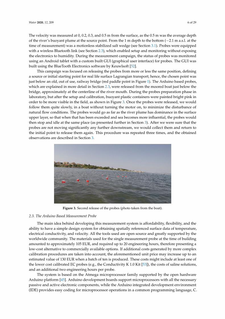
This campaign was focused on releasing the probes from more or less the same position, defininga source or initial starting point for real life surface Lagrangian transport; hence, the chosen point wasjust below an old, out of use, railway bridge (red paddle point in Figure 1). The Arduino based probes,which are explained in more detail in Section 2.3, were released from the moored boat just below thebridge, approximately at the centerline of the river mouth. During the probes preparation phase inlaboratory, but after the setup and calibration, buoyant plastic containers were painted bright pink inorder to be more visible in the field, as shown in Figure 3. Once the probes were released, we wouldfollow them quite slowly, in a boat without turning the motor on, to minimize the disturbance ofnatural flow conditions. The probes would go as far as the river plume has dominance in the surfaceupper layer, so that when that has been exceeded and sea becomes more influential, the probes wouldthen stop and idle at the same place (as presented further in Section 3). After we were sure that theprobes are not moving significantly any further downstream, we would collect them and return tothe initial point to release them again. This procedure was repeated three times, and the obtainedobservations are described in Section 3.

Figure 3. Second release of the probes (photo taken from the boat).

2.3. The Arduino Based Measurement Probe

The main idea behind developing this measurement system is affordability, flexibility, and theability to have a simple design system for obtaining spatially referenced surface data of temperature,electrical conductivity, and velocity. All the tools used are open source and greatly supported by theworldwide community. The materials used for the single measurement probe at the time of buildingamounted to approximately 105 EUR, and required up to 20 engineering hours, therefore presenting alow-cost alternative to commercially available options. If additional costs generated by more complexcalibration procedures are taken into account, the aforementioned unit price may increase up to anestimated value of 130 EUR when a batch of ten is produced. These costs might include at least one ofthe lower cost calibrated EC probes (e.g., the Conductivity K 1.0 Kit [53]), the costs of saline solutions,and an additional two engineering hours per probe.

The system is based on the Atmega microprocessor family supported by the open hardwareArduino platform [45]. Arduino development boards support microprocessors with all the necessarypassive and active electronic components, while the Arduino integrated development environment(IDE) provides easy coding for microprocessor operations in a common programming language, C.

Water 2020, 12, 209 7 of 29

In addition to Arduino development boards, multiple modules were used to perform specific activitiesof the measurement platform. The main organization scheme is given in Figure 4. To provide reliableconnections between components and simplify the field repairs, the motherboard was designed withsimple header connections that require no soldering.

Figure 4. The schematic representation of the Arduino based probe system.

The system can be broken down to these main components: Arduino Mega development board,power management module, SD card logging module, Bluetooth module, temperature measurementmodule, global positioning satellite (GPS) position module, and the newly developed electricalconductivity (EC) module. The Arduino MEGA development board is based on the ATMEGA2560microprocessor [54]. ATMEGA2560 is more robust than ATMEGA328P or ATMEGA32U4, which havebeen used in other variants of Arduino development boards. The main reasons for using ATMEGA2560over other options are the larger program memory size (256 kB vs. 32 kB) and four hardware serial portsthat were necessary for communication with other modules. The ATMEGA2560 is more expensivethan other variants (at the time of writing, unit price was approximately 75% more expensive) but stillwithin the range of affordable solutions.

The power management module was custom made for this application. It consists of a lithium-ionbattery (type 18650, capacity of 2000 mAh), battery protection circuits, and a voltage step-up converter.Used batteries have standardized physical dimensions and satisfactory energy density. The systemwas drawing an average of 250 mAh in use, which enabled a single charge to be active for 8 h. In thecase of a fault (e.g., a short circuit due to water intrusion, overuse, or extreme external heating),the battery protection circuit disconnects the battery to prevent damage. The battery operates at anominal voltage of 3.7 V; hence, a voltage step-up converter is used to increase the voltage to 5 V,as required by all modules in the system. The battery capacity is estimated according to the batteryvoltage, which is measured before the step-up circuit, using an integrated analog digital converter(ADC) in the ATMEGA2560. To have a fixed voltage reference, an internal 1.1 V voltage referenceis used. The battery voltage is scaled using a voltage divider with optimal resistance to minimizebattery drain without interfering with the impedance of ADC. An SD card module is used to recorddata on SD cards for post-measurement data analysis. A Bluetooth module is used for real-time datamonitoring using a PC or mobile phone serial terminal software. This connectivity was used only tospot check the operating drifters without opening the buoy and to download data on demand.

The GPS module is used as both a location device and time keeping device. Specifically, the uBloxNEO-6M module is used to communicate over a serial port using the standard NMEA0183 protocol [55].

Water 2020, 12, 209 8 of 29

Instead of a standard real-time clock, we used GPS modules for time keeping as they ensure timesynchronization between probe units and reduce temporal drift. The NMEA0183 sentence parsingis done via an Arduino TinyGPS library. Temperature and electrical conductivity data are collectedusing a DS18B20 digital temperature sensor [56] and custom made EC module. All of the components,except for the sensing part of temperature and EC module, are contained within a plastic container (seeFigure 5) where the overall volume and mass of the drifter sensor package is made to be half submerged.To prevent the overturning of drifters, the components and additional weights are distributed withinthe container in order to have the center of mass near the center of the bottom plane.

Figure 5. An example of a probe with exposed electrodes below the plastic container (left); and thecalibration procedure in laboratory with the industrial probe (right).

The DS18B20 is in a standard TO-92 package but sealed in a thin, stainless steel cylinder enclosurefor protection against salt water intrusion. Such sensors have a typical accuracy of ±0.5 °C inmeasurement range from −10 to 85 °C. For our intended applications, where the temperature range isrestricted in the range of 15–30 °C, characteristic accuracy was 0.1–0.2 °C.

The electrical conductivity measurement module is constructed from the Arduino Pro Microdevelopment board, and a monolithic H-bridge for driving alternative currents and passivecomponents as low pass filters. The exposed surfaces of gold-plated printed circuit boards (PCBs), i.e.,electrodes, were used as active sensors (Figure 6). The module has three pairs of electrodes to enhancesensitivity for measurements in a low conductivity medium. In brackish water, only one pair wasneeded. The other two pairs were insulated using a double coat of clear acrylic lacquer (PLASTIK 70).The single sensing pair has a surface of 15 mm2 and are set 10 mm apart.

Figure 6. The printed circuit board (PCB) for the electrical conductivity sensor.

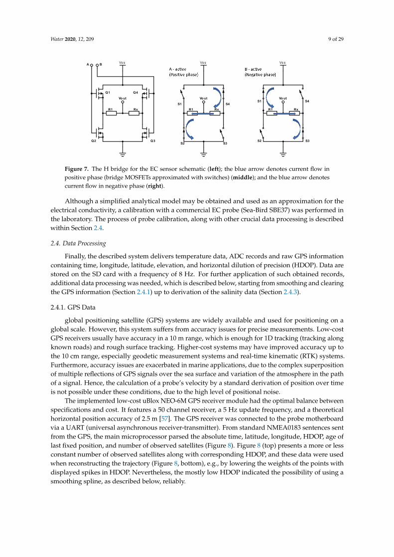
The operating principle of the module is as follows: by using the H-bridge (Q1 to Q4 in Figure 7),the alternating voltage is applied on the series connector between the known value resistor and theactive sensors inserted into the medium. This connection between known resistance (R1 in Figure 7) andresistance across sensing surfaces (Rx in Figure 7) forms a voltage divider that enables the correlationof voltage measured between resistors and the resistance of the unknown medium. The output of thevoltage divider (Vout in Figure 7) is routed to the ADC of the Arduino Pro Mini. The measurement iscarried out only in the positive phase of the cycle, while the negative voltage phase is used to preventelectrolysis near the sensor surface, which would contaminate the measurement surface.

Water 2020, 12, 209 9 of 29

Figure 7. The H bridge for the EC sensor schematic (left); the blue arrow denotes current flow inpositive phase (bridge MOSFETs approximated with switches) (middle); and the blue arrow denotescurrent flow in negative phase (right).

Although a simplified analytical model may be obtained and used as an approximation for theelectrical conductivity, a calibration with a commercial EC probe (Sea-Bird SBE37) was performed inthe laboratory. The process of probe calibration, along with other crucial data processing is describedwithin Section 2.4.

2.4. Data Processing

Finally, the described system delivers temperature data, ADC records and raw GPS informationcontaining time, longitude, latitude, elevation, and horizontal dilution of precision (HDOP). Data arestored on the SD card with a frequency of 8 Hz. For further application of such obtained records,additional data processing was needed, which is described below, starting from smoothing and clearingthe GPS information (Section 2.4.1) up to derivation of the salinity data (Section 2.4.3).

2.4.1. GPS Data

global positioning satellite (GPS) systems are widely available and used for positioning on aglobal scale. However, this system suffers from accuracy issues for precise measurements. Low-costGPS receivers usually have accuracy in a 10 m range, which is enough for 1D tracking (tracking alongknown roads) and rough surface tracking. Higher-cost systems may have improved accuracy up tothe 10 cm range, especially geodetic measurement systems and real-time kinematic (RTK) systems.Furthermore, accuracy issues are exacerbated in marine applications, due to the complex superpositionof multiple reflections of GPS signals over the sea surface and variation of the atmosphere in the pathof a signal. Hence, the calculation of a probe’s velocity by a standard derivation of position over timeis not possible under these conditions, due to the high level of positional noise.

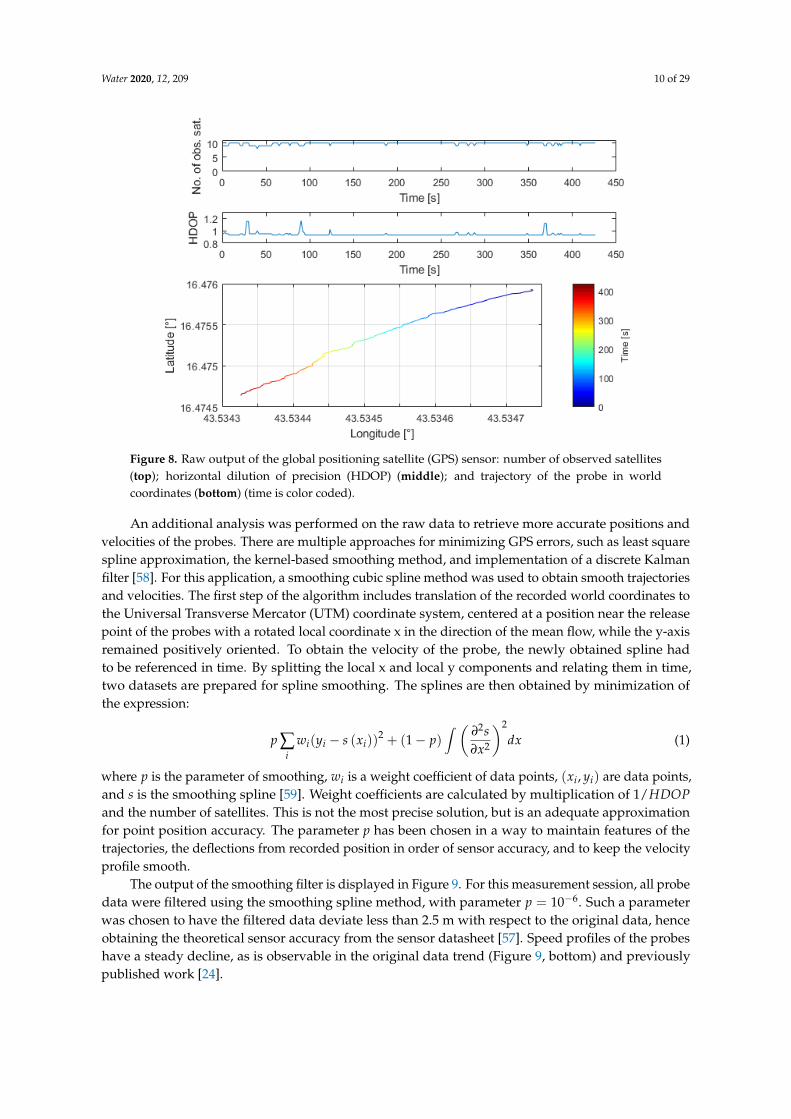
The implemented low-cost uBlox NEO-6M GPS receiver module had the optimal balance betweenspecifications and cost. It features a 50 channel receiver, a 5 Hz update frequency, and a theoreticalhorizontal position accuracy of 2.5 m [57]. The GPS receiver was connected to the probe motherboardvia a UART (universal asynchronous receiver-transmitter). From standard NMEA0183 sentences sentfrom the GPS, the main microprocessor parsed the absolute time, latitude, longitude, HDOP, age oflast fixed position, and number of observed satellites (Figure 8). Figure 8 (top) presents a more or lessconstant number of observed satellites along with corresponding HDOP, and these data were usedwhen reconstructing the trajectory (Figure 8, bottom), e.g., by lowering the weights of the points withdisplayed spikes in HDOP. Nevertheless, the mostly low HDOP indicated the possibility of using asmoothing spline, as described below, reliably.

Water 2020, 12, 209 10 of 29

Figure 8. Raw output of the global positioning satellite (GPS) sensor: number of observed satellites(top); horizontal dilution of precision (HDOP) (middle); and trajectory of the probe in worldcoordinates (bottom) (time is color coded).

An additional analysis was performed on the raw data to retrieve more accurate positions andvelocities of the probes. There are multiple approaches for minimizing GPS errors, such as least squarespline approximation, the kernel-based smoothing method, and implementation of a discrete Kalmanfilter [58]. For this application, a smoothing cubic spline method was used to obtain smooth trajectoriesand velocities. The first step of the algorithm includes translation of the recorded world coordinates tothe Universal Transverse Mercator (UTM) coordinate system, centered at a position near the releasepoint of the probes with a rotated local coordinate x in the direction of the mean flow, while the y-axisremained positively oriented. To obtain the velocity of the probe, the newly obtained spline hadto be referenced in time. By splitting the local x and local y components and relating them in time,two datasets are prepared for spline smoothing. The splines are then obtained by minimization ofthe expression:

p ∑i

wi(yi − s (xi))2 + (1− p)

∫ (∂2s∂x2

)2

dx (1)

where p is the parameter of smoothing, wi is a weight coefficient of data points, (xi, yi) are data points,and s is the smoothing spline [59]. Weight coefficients are calculated by multiplication of 1/HDOPand the number of satellites. This is not the most precise solution, but is an adequate approximationfor point position accuracy. The parameter p has been chosen in a way to maintain features of thetrajectories, the deflections from recorded position in order of sensor accuracy, and to keep the velocityprofile smooth.

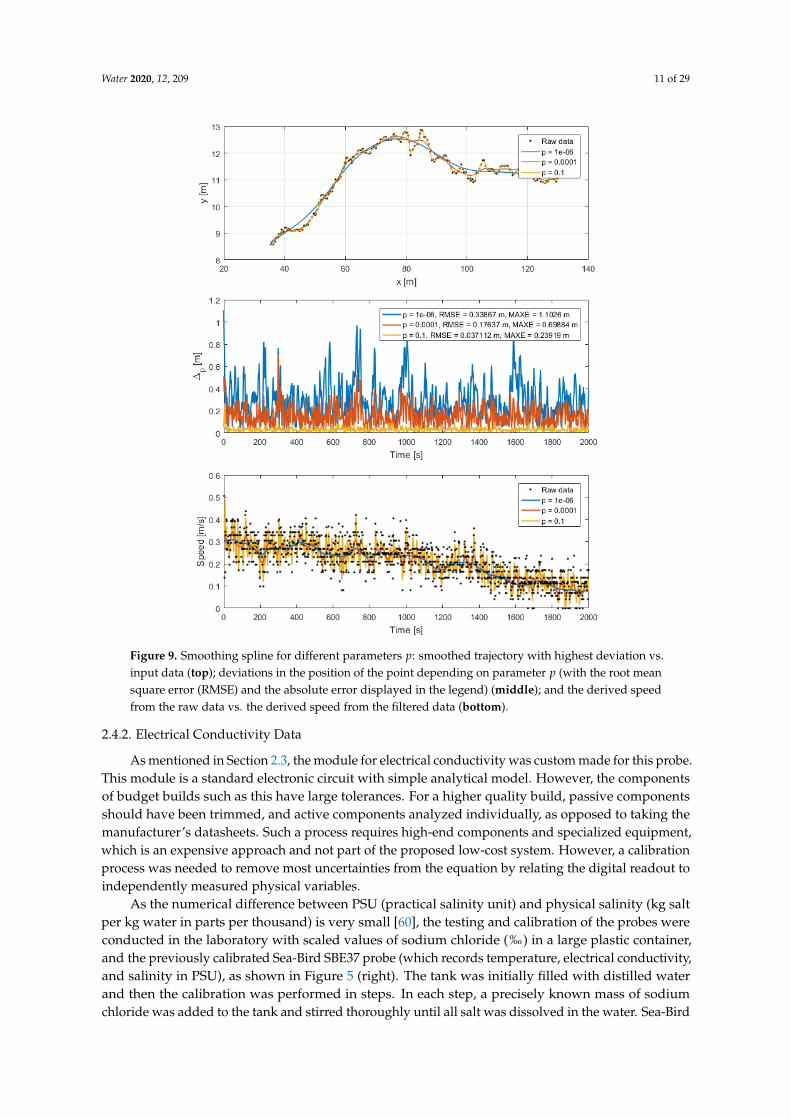
The output of the smoothing filter is displayed in Figure 9. For this measurement session, all probedata were filtered using the smoothing spline method, with parameter p = 10−6. Such a parameterwas chosen to have the filtered data deviate less than 2.5 m with respect to the original data, henceobtaining the theoretical sensor accuracy from the sensor datasheet [57]. Speed profiles of the probeshave a steady decline, as is observable in the original data trend (Figure 9, bottom) and previouslypublished work [24].

Water 2020, 12, 209 11 of 29

Figure 9. Smoothing spline for different parameters p: smoothed trajectory with highest deviation vs.input data (top); deviations in the position of the point depending on parameter p (with the root meansquare error (RMSE) and the absolute error displayed in the legend) (middle); and the derived speedfrom the raw data vs. the derived speed from the filtered data (bottom).

2.4.2. Electrical Conductivity Data

As mentioned in Section 2.3, the module for electrical conductivity was custom made for this probe.This module is a standard electronic circuit with simple analytical model. However, the componentsof budget builds such as this have large tolerances. For a higher quality build, passive componentsshould have been trimmed, and active components analyzed individually, as opposed to taking themanufacturer’s datasheets. Such a process requires high-end components and specialized equipment,which is an expensive approach and not part of the proposed low-cost system. However, a calibrationprocess was needed to remove most uncertainties from the equation by relating the digital readout toindependently measured physical variables.

As the numerical difference between PSU (practical salinity unit) and physical salinity (kg saltper kg water in parts per thousand) is very small [60], the testing and calibration of the probes wereconducted in the laboratory with scaled values of sodium chloride (‰) in a large plastic container,and the previously calibrated Sea-Bird SBE37 probe (which records temperature, electrical conductivity,and salinity in PSU), as shown in Figure 5 (right). The tank was initially filled with distilled waterand then the calibration was performed in steps. In each step, a precisely known mass of sodiumchloride was added to the tank and stirred thoroughly until all salt was dissolved in the water. Sea-Bird

Water 2020, 12, 209 12 of 29

SBE37 was used to monitor the dissolving process simultaneously. The conductivity sensing part ofthe probe was at the same depth as Sea-Bird’s sensor, to reduce the effects of salt distribution overdepth. Finally, each probe was set in the water, connected to a tablet via Bluetooth, and multipleconductivity digital output and temperature readings were recorded for further analysis. The rangeof salinity was 0–34 ppt, divided into 10 steps. The monitored temperature was steady and accurateduring the process (the same value was recorded by the proposed probe’s temperature sensor andSea-Bird’s sensor).

A calibration analysis was done after acquiring data for all 10 steps described above.The systematic errors were removed (such as trapped air on the surface of the sensor, communicationerrors, etc.), then the averaged reading for every salinity level and for every probe was obtained,and finally an appropriate curve was fitted to the measured data points. The equation finally used forfitting the measured data was:

EC [S/m] = a · Xb (2)

where EC is the real electrical conductivity in S/m while X is the averaged and cleaned digital readoutfrom the Arduino ADC (0 is equal to 0 V, and 1023 is equal to 5 V). Parameters a and b were obtainedfrom a function fitting procedure using the nonlinear least square method. Finally, fitting curves wereobtained along with measures of goodness of fit. The typical four metrics are displayed in Figure 10.The adjusted R2 metric describes how the function was chosen, taking into account degrees of freedom(number of data) for fit. Values, for all probes, are above 0.85, which indicates that appropriatefunctions were chosen. Next, two metrics, root mean square error (RMSE) and mean absolute error(MAE), describe typical errors from measurement. The difference of these two metrics are that largerdeviations have a stronger effect on RMSE, while MAE linearly combines all errors. Furthermore,absolute errors have been normalized by corresponding measured values and averaged over allmeasurements per probe. Such a metric, namely averaged relative error (Figure 10, right), gives anequal importance over the whole measuring range.

Finally, the MAE for all probes was less than 0.1 S/m while RMSE was less than 0.5 S/m.In Figure 11, a distribution of absolute error averaged over probes for different values of salinity isshown. One may notice that most of the errors are in the area with higher salinity, as expected fromthe architecture of the measurement system. By reducing the range of measurement to 25 PSU, we canobtain much smaller error metrics. This reduction in range did not limit our usability of probes, sincethe target area of the estuary exhibits significantly lower salinity than the open sea (in the Adriatic Sea,salinity is around 38 PSU), 20 PSU at the mesohaline estuary.

Figure 10. The metrics of calibration.

Water 2020, 12, 209 13 of 29

Figure 11. The distribution of mean absolute error for all probes for different salinity levels.

2.4.3. Salinity Data

Following the process, which is usually implemented in off-the shelf solutions, we have introducedthe sensors for temperature and electrical conductivity (EC). EC was obtained from the ADC output,as explained in Section 2.3. Once the temperature and electrical conductivity were obtained, the salinitywas calculated using the practical salinity scale (PSS) derived in 1978 by Perkin and Lewis:

S =5

∑j=0

ajR1/2T +

(T − 15)1 + k (T − 15)

5

∑j=0

bjR1/2T . (3)

In Equation (3), Rt = R/(RPrT) where R = EC(S, T, P)/EC(35, 15, 0) is the electrical conductivityratio between the measured value and the baseline for the standard potassium chloride (KCl) solutionat 35 ppt, 15 ◦C, and 0 pressure in decibars, while RP and rT are calibrated factors of measured pressureand temperature, respectively. Our data were measured at the surface due to the design purpose ofprobes, thus the P in R is zero all the time. For the salinity calculation, we used the same baselineconductivity value as the Sea-Bird SBE37, i.e., EC(35, 15, 0) = 42.914 dS/m. The parameter k has thevalue of 0.0162 for the ranges of salinity between 2 and 42 PSU, and temperature between −2 ◦C and35 ◦C, while aj and bj are fitting parameters defined by the practical salinity scale (PSS) equations from1978. More on the PSS equations may be found in [61].

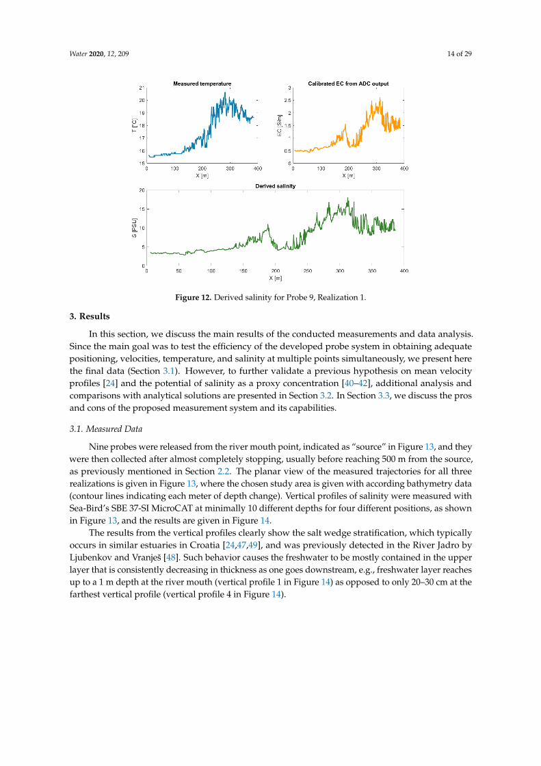
An example for the explained data is given in Figure 12 for the ninth probe in the first realization(first release of the probes). The corresponding datasets for temperature (Figure 12, top left), electricalconductivity (Figure 12, top right), and salinity derived by Equation (3) are shown for the lengthof the probe’s trajectory (a little less than 400 m from the source). Salinity clearly depends on bothtemperature and conductivity; however, conductivity has a dominating effect, as depicted by the shapeof the curve itself (Figure 12).

Water 2020, 12, 209 14 of 29

Figure 12. Derived salinity for Probe 9, Realization 1.

3. Results

In this section, we discuss the main results of the conducted measurements and data analysis.Since the main goal was to test the efficiency of the developed probe system in obtaining adequatepositioning, velocities, temperature, and salinity at multiple points simultaneously, we present herethe final data (Section 3.1). However, to further validate a previous hypothesis on mean velocityprofiles [24] and the potential of salinity as a proxy concentration [40–42], additional analysis andcomparisons with analytical solutions are presented in Section 3.2. In Section 3.3, we discuss the prosand cons of the proposed measurement system and its capabilities.

3.1. Measured Data

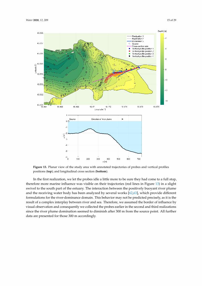
Nine probes were released from the river mouth point, indicated as “source” in Figure 13, and theywere then collected after almost completely stopping, usually before reaching 500 m from the source,as previously mentioned in Section 2.2. The planar view of the measured trajectories for all threerealizations is given in Figure 13, where the chosen study area is given with according bathymetry data(contour lines indicating each meter of depth change). Vertical profiles of salinity were measured withSea-Bird’s SBE 37-SI MicroCAT at minimally 10 different depths for four different positions, as shownin Figure 13, and the results are given in Figure 14.

The results from the vertical profiles clearly show the salt wedge stratification, which typicallyoccurs in similar estuaries in Croatia [24,47,49], and was previously detected in the River Jadro byLjubenkov and Vranješ [48]. Such behavior causes the freshwater to be mostly contained in the upperlayer that is consistently decreasing in thickness as one goes downstream, e.g., freshwater layer reachesup to a 1 m depth at the river mouth (vertical profile 1 in Figure 14) as opposed to only 20–30 cm at thefarthest vertical profile (vertical profile 4 in Figure 14).

Water 2020, 12, 209 15 of 29

Figure 13. Planar view of the study area with annotated trajectories of probes and vertical profilespositions (top); and longitudinal cross section (bottom).

In the first realization, we let the probes idle a little more to be sure they had come to a full stop,therefore more marine influence was visible on their trajectories (red lines in Figure 13) in a slightswivel to the south part of the estuary. The interaction between the positively buoyant river plumeand the receiving water body has been analyzed by several works [62,63], which provide differentformulations for the river-dominance domain. This behavior may not be predicted precisely, as it is theresult of a complex interplay between river and sea. Therefore, we assumed the border of influence byvisual observation and consequently we collected the probes earlier in the second and third realizationssince the river plume domination seemed to diminish after 300 m from the source point. All furtherdata are presented for those 300 m accordingly.

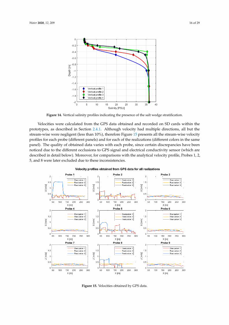
Water 2020, 12, 209 16 of 29

Figure 14. Vertical salinity profiles indicating the presence of the salt wedge stratification.

Velocities were calculated from the GPS data obtained and recorded on SD cards within theprototypes, as described in Section 2.4.1. Although velocity had multiple directions, all but thestream-wise were negligent (less than 10%), therefore Figure 15 presents all the stream-wise velocityprofiles for each probe (different panels) and for each of the realizations (different colors in the samepanel). The quality of obtained data varies with each probe, since certain discrepancies have beennoticed due to the different occlusions to GPS signal and electrical conductivity sensor (which aredescribed in detail below). Moreover, for comparisons with the analytical velocity profile, Probes 1, 2,5, and 8 were later excluded due to these inconsistencies.

Figure 15. Velocities obtained by GPS data.

Water 2020, 12, 209 17 of 29

Temperature is an important property in any water resources due to its effect on the levelof dissolved oxygen [64–66] and consequently on the existing biome there. In estuaries, due totheir dynamic nature, the temperature fluctuates, and additional variations occur when potentialgroundwater discharges, precipitation, or insolation are present. Since the temperature sensor wasmore or less insensitive to all the potential environmental conditions (e.g., an air bubble stuck at theelectrical conductivity sensor), recorded temperature data are rather consistent with the expectedphysical behavior (see Figure 16). For the first 100 m from the source point, most of the probes recordeda consistent river surface temperature in the range of 15–16 °C (also consistent with some of theprevious measurements for the River Jadro during summer [48]). Afterward, temperature slowlystarted to fluctuate as the sea water influence increases (at 150 m from source), finally reaching theambient sea temperature of around 21–22 °C, in Kaštela Bay. The X distance in the figure, again,represents the stream-wise direction, which does not necessarily mean the straight line from the sourcebut rather a trajectory. However, for most probes, the first realization had the furthest distance, hencethe red line in Figure 16 reaches the ambient temperature. The first realization’s trajectories also reachmore salty water due to the inclination of the plume centerline, hence exiting the river plume soonerthan the probes in the two other realizations.

Probe 8 experienced a lack of data in Realizations 1 and 3 (after 200 m), most likely due to a lostGPS lock that stopped the recording. The same probe in the second realization experienced rather lowvalues (compared to the other probes), as its trajectory was mainly in the plume centerline, thereforerecording mostly river dominated temperatures (16–18 °C), which are lower than the temperature ofthe ambient coastal sea (21–22 °C). Probe 2, for instance, lost information for the last realization at lessthan 200 m, which was caused by battery depletion. These data losses for Probes 2 and 8 are visible inall sensor’s data in the third realization (see the corresponding panels in Figures 15–17).

Figure 16. Measured temperature.

Water 2020, 12, 209 18 of 29

Figure 17. Measured electrical conductivity (EC). Analog digital converter (ADC).

The electrical conductivity sensor, as expected, was shown to be the most sensitive one.As described in Sections 2.3 and 2.4, it is a plate with one pair of active electrodes in the form ofkeel below the plastic container, which acts as a mini-floater. The keel enabled the mini-floater to bemore stabilized in the water; however, when surface rips were caused by occasional light wind blows,sporadic vegetation, and local waves emanating from passing boats, some of the air got stuck betweenthe keel and the plastic container, rendering the EC measurement useless. Two probes, namely Probes4 and 6, experienced total failure in recording the EC. Later, we discovered that water had entered thepart of the EC module circuit (positioned on the keel) that was insufficiently water-proofed.

Nevertheless, the expected behavior of electrical conductivity (EC) was still observed in the restof the probes.

Finally, salinity data for each probe were obtained by implementing the calculation described inSection 2.4.3, as presented in Figure 18.

As already established, there are no significant differences between conductivity andsalinity behavior trends, as salinity was obtained from Equation (3), with domination of theconductivity’s influence.

Water 2020, 12, 209 19 of 29

Figure 18. Measured salinity in practical salinity units (PSU).

3.2. Application Potential

An important application of the research was tested by comparing the velocity data withpreviously defined analytical expressions (Equation (4)). In addition, both salinity and temperaturewere tested as potential concentration proxies for conservative solutes.

3.2.1. Velocity Model

In our previous research, several measurements were conducted at the River Žrnovnica,as explained in [24,41], and, from those results, an approximation for the depth-integrated meanvelocity U in the near-field area of an estuary and a steady source was given:

U(x) = U0e−νx (4)

where U0 is the cross-sectionally averaged velocity at the river mouth and ν [m−1] is an attenuationcoefficient representing all potential mechanisms (bathymetry, tides, wind, etc.) that, when combined,concur to progressively reduce U in the x direction [42].

The proposed exponential attenuation model for mean velocity was already tested and comparedto the existing theoretical model for jet flow [67] and hydrodynamic model MOHID [68]. However,the intent was to obtain an easier way to measure downstream velocities simultaneously and obtainthe attenuation coefficient ν [m−1]. Hence, in each realization (different panels in Figure 19), aregression analysis was applied (using the root mean square error) to find the optimal parameters,U0 and ν, for each probe. The final values in figures are averaged for all corresponding probes ina realization. As mentioned above, not all probes succeeded in obtaining the relevant velocity datain each realization (due to technical difficulties), which is why their velocity profiles were not takeninto account. Nevertheless, parameters were obtained, including the initial velocity, in a range from0.3 to 0.37 m/s, which is close to 0.29 m/s, measured by hydrometric wing (Section 2.2), and havingan attenuation coefficient in a rather low range from 0.0003 to 0.0022 m−1. The velocity obtained by

Water 2020, 12, 209 20 of 29

the presented probe system is strictly a surface one. However, since the studied estuary is stratified,most of the flow is contained in the upper river’s buoyant plume that becomes thinner along thedownstream direction. This is also a reason for a slightly higher initial velocity obtained by the fittingprocedure described above. The attenuation coefficient is low due to the steady conditions in theestuary with little or no wind at all, and small tide conditions in the already very closed Kaštela Bay,and therefore quite limited impact of the velocity attenuation. Moreover, in this case, one may considerthe mean velocity to be constant in the near-field zone of the corresponding estuary.

Figure 19. Velocity model parameters.

3.2.2. Concentration Proxy

Both temperature and salinity epitomize crucial parameters in an estuary, from their physicalvariability to the impact they cause on hydrodynamic conditions as well as the estuarine biome. Due tosuch importance, and thanks to the current and rising measurement abilities, those two properties areamong the most monitored and used data, which makes them an attractive alternative for emulationof an actual, mostly conservative, solute transport. Several studies used salinity [33,35,36,38,39] ortemperature [33,69,70] as an indicator for other properties in rivers and estuaries. Hence, sea waterdilution (supported by both salinity and temperature data) may be considered as an inverse processto river transport by freshwater discharge, as freshwater both dilutes the salinity and decreases thetemperature. Salinity was proposed in [40–42] as a proxy for normalized concentration in the surfacewater layer:

CSp(x, t) = 1− S(x, t)− Smin

Smax − Smin(5)

Water 2020, 12, 209 21 of 29

where S(x, t) is the measured surface salinity value at point x and time t, Smin is the initial salinitymeasured at the river mouth (considered to be the minimal one at the area of interest), and Smax

represents the ambient sea surface salinity in the estuary. Such utilization of salinity data may bepossible only when the steady-state assumption is valid, such as when other factors (e.g., windcurrents and tides) have a minimal effect on the estuary [35]. To ensure steadiness in both flow andwater levels of the river, an adequate time period from the most recent precipitation was required.Therefore, weather forecast and tide predictions were taken into account when choosing dates for themeasurement campaigns.

Furthermore, temperature seemed to have a similar behavior, thus the same procedure defined byEquation (5) was applied to temperature data, including the choice of minimal surface temperature Tminas the initial one (at the river mouth) and Tmax as the ambient sea surface temperature in the estuary:

CTp (x, t) = 1− T(x, t)− Tmin

Tmax − Tmin. (6)

When wakes, jets, and plumes are considered, a Gaussian one-dimensional distribution may beassumed for cross-sectional profiles [71–73]. In our previous research, we applied such definition ofsolute mean concentration on a plane normal to the mean flow direction for the near-field zone of anestuary exhibiting steady flow with a steady source [24,40,42,74]:

c (y, x) =L

σy√

2πe−y2

2σ2y (7)

where L = mBU0

is a steady mass loading of the solute through the plane normal to the flow directionx, defined by steady mass flux (m), river mouth width (B), and the initial velocity (U0). The spatialvariance is defined by σ2

y = 2ett + σ2y0

, x = Ut, where et (m2/s) is the constant spatial variance growthrate (equivalent to turbulent diffusivity) across the flow in the direction y, and σ2

y0represents the initial

variance at x = 0.On that note, we wanted to test how well the measured data match the assumed Gaussian

analytical model, and if so, what parameters might be obtained for further analytical modeling.Measured temperature and salinity, as described in Section 2, were sampled with an 8 Hz frequency,and with a velocity of probes ranging from 0.4 to 0.2 m/s (Figure 15). We obtained 20–40 pointsper 1 m of probe trajectory. By taking trajectories for all three releases of probes (realizations), bothsalinity and temperature proxy data were obtained (using Equations (5) and (6)) and surface fittedby Gaussian distribution (Equation (7)). In Figure 20, we present the aforementioned surface fit forboth temperature proxy concentration (Figure 20, top) and for salinity proxy concentration (Figure 20,bottom) with corresponding parameters and the statistics for goodness of fit (R2 and RMSE). Theparameters that were optimized to obtain the fit are spatial variance growth rate (et), effective sourcewidth or initial spatial variance (σy0 ), and the angle (α). α represents the rotation of the local coordinatesystem with regards to the UTM coordinates as presented:

x = (xUTM − xUTM,0) cos α− (yUTM − yUTM,0) sin α

y = (xUTM − xUTM,0) sin α + (yUTM − yUTM,0) cos α (8)

where xUTM,0 and yUTM,0 are corresponding UTM coordinates of the source. The obtained fit slightlybetter presents the proxy defined by salinity with the coefficient of determination, R2 = 0.803 versusR2 = 0.749 for temperature proxy. Similarly, the residuals for temperature proxy are more spread outfrom the Gaussian fit with RMSE = 0.123, which is an almost two times larger scattering than withthe salinity proxy (RMSE = 0.0777). In addition, it should be noted that, although temperature andsalinity are measured through different devices, the fitted parameters, i.e., et = 0.143 m2/s and α = 200for temperature and et = 0.0856 m2/s and α = 198 for salinity, are on the same order of magnitude.

Water 2020, 12, 209 22 of 29

This evidence gives more reliability to our data, which are able to picture the main physical behaviorof the contaminant dispersion in the estuary environment.

Figure 20. Comparison between the measured data and Gaussian mean distribution for: salinity as aconcentration proxy (top); and temperature as a concentration proxy (bottom).

Conclusively, this procedure has confirmed our previous work on using salinity as a proxy forconservative solute transport when compared with analytical solutions for mean concentration in asteady state with a steady source. However, an unexpected bonus from this procedure was the optionfor obtaining the spatial variance growth rate, which is equivalent to turbulent diffusivity and one ofthe physical parameters that is very difficult to measure, directly or otherwise [21,75].

3.3. Discussion and Lessons Learned

To test the behavior and variability of measured temperature and salinity data within the proposedmeasurement system, a corresponding coefficient of variation (CV) was calculated. The coefficient ofvariation is defined as the ratio between the standard deviation to the mean and, therefore, it is used toquantify the degree of dispersion of a sample. The CV of temperature and salinity for all trajectories ineach realization is presented in Figure 21.

Water 2020, 12, 209 23 of 29

Figure 21. Coefficient of variation (CV) for temperature and salinity in the down stream direction.

The results show an expected low level (less than 10%) of temperature variability between theprobes and realizations, confirming that the temperature has stable behavior. Conversely, salinityexhibits rather high variability. Even though this high variability is partially a function of a conductivitysensor being more susceptible to environmental conditions, it also confirms the higher dispersion thatboth conductivity and salinity exhibit in the estuary where mixing is an important feature [71,76,77].

As already established, the conditions in the investigated estuary belong to a predominantlystationary process, and therefore we used the fast Fourier transform of normalized temperature,conductivity, and salinity data to obtain the power spectral density (PSD) estimate [78,79]. Hence,in Figure 22, single-sided PSDs are shown.

The key finding related to the spectral domain (Figure 22) implies that the salinity measuredby developed probes is not simply an unorganized random field (in the case the PSD was showinga constant line over all available frequencies), but rather distributed over lower frequencies (e.g.,0–0.15 Hz); therefore, the variability was a function of long period changes, which is consistent withthe examined physical problem. The presented signal also resembles a pink noise with an almostsystematic reduction of PSD along the frequencies. As expected, since EC is a more influential variablethan temperature in Equation (3), salinity variance is more aligned to the EC variance (see Figure 22).

To apply this measurement system, a steady state should be established. When steady stateconditions are met, one may consider the salinity behavior equivalent to a conservative tracer transportcoming from the river. This steady-state assumption has been proven by steady velocity profiles(Figure 19) and the PSDs above (Figure 22). On the other hand, if probes are going to be used asLagrangian style surface drifters (similar to [46]), they represent cheap and efficient tracers in anyenvironmental conditions; however, the GPS precision should be improved by implementation of RTK(real-time kinematic) system GPS, or by adding additional inertial measurement systems. Furthermore,to have adequate conductivity/salinity measurements in that system, some weight to probe containersshould be added along with better keel shaping to avoid air bubbles below them (which causedour conductivity data stream to be interrupted). The parts of the EC circuit that are positioned ona keel should be meticulously tested for being water proof, in order to avoid the problems that weencountered in the field (Probes 4 and 6).

Water 2020, 12, 209 24 of 29

Figure 22. Power spectral density (PSD) of normalized fluctuations for temperature (T), electricalconductivity (EC), and salinity (S) in Realization 1.

However, using the salinity data as a concentration proxy for conservative solute becomeschallenging, since the mixing in higher waves, or increased sea current effects, would become morepronounced, hence diminishing the river domination as a key assumption for using the analyticalmodels by Galešic et al. [24], Andricevic and Galešic [40]. Nevertheless, if successful, all acquired datamay be very useful for describing hydrodynamics in the estuary in different conditions, which may belater compared to numerical models, and even help in calibrating them.

4. Conclusions and Future Remarks

In this paper, we present an innovative low-cost measurement system for surface water properties.At the time of the development, the resources needed for building one probe included approximately130 EUR of materials and up to 22 h of engineering work. These costs are two orders of magnitudelower than corresponding off-the-shelf solutions, which additionally require significant modificationsto fit specific application needs.

Furthermore, an important goal of this study was to test if the proposed system of probes issatisfactory to obtain quality data on temperature, salinity, and velocities in the near field zone of anestuary. The obtained results deliver promising functionality for surface salinity data, downstreamsurface velocities, and surface temperature. However, for more detailed and depth-related informationon salinity, researchers would need different equipment. Thanks to the multiple probe-releasing option,the velocity field is rather easily obtained from GPS data. The measured velocity is in agreementwith the attenuation model proposed by Galešic et al. [24]. Moreover, one may obtain the velocityattenuation coefficient in this way with only one realization by averaging the velocity profiles of allprobes. As expected, several problems were detected, starting from the electrical conductivity sensor,

Water 2020, 12, 209 25 of 29

which should be made more range oriented, i.e., if salinity is expected to appear out of the range2–25 PSU, the corresponding electrodes (as presented in Figure 6) should have multiple sensitivityreal-time switchable settings.

Furthermore, this kind of free probe-release is best applied to steady and calm surface conditions.Otherwise, sudden waves resulting from passing boats, birds, or wind may interfere with the dataacquisition. However, such stabilization problems might be solved with different keel shaping andby adding some additional weight to the probe. Lithium-ion batteries have shown to be an effectivesolution for these short term measurements (up to 8 h, which is more than the relatively steadyconditions may appear anyway), although they should be frequently checked. In addition, an ideawas brought to attention while processing GPS data to obtain velocity: one may include the inertialmeasurement units (IMU), such as accelerometers, gyrometers, and magnetometers, to have morequality and controlled information.

The presented prototype may be one of the first steps toward development of a more complexmonitoring system applicable in a broader range of conditions, which has potential for furtherresearch. However, it is important to emphasize that this drifter system was specifically developed tosimultaneously obtain data on surface salinity concentrations in multiple points, in order to improvethe validation of analytical models for conservative solute transport (both Galešic et al. [24] andAndricevic and Galešic [40]). Currently ongoing research includes the analysis of data when probeswere fixed on chosen stream-wise or cross-stream profiles, therefore obtaining rich datasets at multiplepoints (measurements conducted on 12 and 13 July 2018). Data at fixed points enable testing thestatistics with analytical models for both point defined statistics (probability density functions andtheir moments) and spatially integrated statistics (expected mass fraction and spatially integratedmoments). Since typical tracer releases (e.g., [22]) are difficult, expensive, and time consuming toobtain adequate statistics, salinity emerged as a convenient proxy.

The aforementioned models analyzed the worst-case scenario where the lack of wind stress andhigh tides reduce dilution of conservative pollution generated by the river. Therefore, the measurementconditions were chosen during low tide and low winds on purpose.

Among the future research directions is also the integration of measured data within MSDIaccording to the INSPIRE Directive and associated regulations. Data from different sensors, as well asdata from other sources, might be integrated to create a comprehensive data web stream for analysis,which should yield more precise and accurate data models.

Author Contributions: Conceptualization, V.D., M.G., M.D.D., M.T., and R.A.; Funding acquisition, M.G. andR.A.; Investigation, V.D., M.G., M.D.D., and M.T.; Methodology, V.D., M.G., M.D.D., and R.A.; Visualization, M.G.,M.D., and M.T.; Writing—original draft, V.D. and M.G.; and Writing—review and editing, M.D.D., M.T., and R.A.All authors have read and agreed to the published version of the manuscript.

Funding: This research was partially supported through project KK.01.1.1.02.0027, a project co-financedby the Croatian Government and the European Union through the European Regional DevelopmentFund—the Competitiveness and Cohesion Operational Programme, Contract Number: KK.01.1.1.02.0027.Additionally, the research was supported by next two projects: STIM-REI (Center of Excellence for Scienceand Technology–Integration of Mediterranean Region (STIM), connecting research (R), education (E) andinnovation (I)), a project funded by European Union from European Structural and Investment Funds 2014.–2020.,Contract Number: KK.01.1.1.01.0003, and CAAT (Coastal Auto-purification Assessment Technology) alsofunded by European Union from European Structural and Investment Funds 2014.–2020., Contract Number:KK.01.1.1.04.0064.

Acknowledgments: We thank Koca Vrancic for important help during the development of the prototype formeasurement system. Furthermore, we thank Ana Ricov for valuable help during the measurement campaigns.

Conflicts of Interest: The authors declare no conflict of interest.

Water 2020, 12, 209 26 of 29

References

1. Elliott, M.; Whitfield, A.K. Challenging paradigms in estuarine ecology and management. Estuar. Coast.Shelf Sci. 2011, 94, 306–314. doi:10.1016/j.ecss.2011.06.016.

2. Halpern, B.S.; Walbridge, S.; Selkoe, K.A.; Kappel, C.V.; Micheli, F.; D’agrosa, C.; Bruno, J.F.; Casey, K.S.;Ebert, C.; Fox, H.E.; et al. A global map of human impact on marine ecosystems. Science 2008, 319, 948–952.

3. Wolanski, E.; Elliott, M. Estuarine Ecohydrology: An Introduction; Elsevier: Amsterdam, the Netherlands, 2015.4. Assessment, M.E. Ecosystems and Human Well-Being; Island Press: Washington, DC, USA, 2005; Volume 5.5. Barbier, E.B.; Hacker, S.D.; Kennedy, C.; Koch, E.W.; Stier, A.C.; Silliman, B.R. The value of estuarine and

coastal ecosystem services. Ecol. Monogr. 2011, 81, 169–193. doi:10.1890/10-1510.1.6. Barbier, E.B. Progress and Challenges in Valuing Coastal and Marine Ecosystem Services. Rev. Environ. Econ.

Policy 2011, 6, 1–19. doi:10.1093/reep/rer017.7. Milon, J.W.; Alvarez, S. The Elusive Quest for Valuation of Coastal and Marine Ecosystem Services. Water

2019, 11, 1518. doi:10.3390/w11071518.8. Copeland, C. Clean Water Act: A Summary of the Law; Congressional Research Service, Library of Congress:

Washington, DC, USA, 1999.9. European Community. Directive 2000/60/EC of the European Parliament and of the Council of 23 October 2000

Establishing a Framework for Community Action in the Field of Water Policy; Official Journal of the EuropeanCommunities (L 327/1-73); European Community: Brussels, Belgium, 2000.

10. European Community. Bathing Water Quality Directive 2006/7/EC; Official Journal of the European Union(OJ L 64); European Community: Brussels, Belgium, 2006.

11. European Community. Directive 2008/56/EC of the European Parliament and of the Council of 17 June 2008Establishing a Framework for Community Action in the Field of Marine Environmental Policy (Marine StrategyFramework Directive); Official Journal of the European Union (L 164/19-40); European Community: Brussels,Belgium, 2008.

12. Guerry, A.D.; Plummer, M.L.; Ruckelshaus, M.H.; Harvey, C.J. Ecosystem service assessments for marineconservation. In Natural Capital: Theory and Practice of Mapping Ecosystem Services; Oxford University Press:Oxford, UK, 2011; pp. 296–322.

13. Pinto, R.; de Jonge, V.N.; Neto, J.M.; Domingos, T.; Marques, J.C.; Patrício, J. Towards a DPSIR drivenintegration of ecological value, water uses and ecosystem services for estuarine systems. Ocean. Coast.Manag. 2013, 72, 64–79. doi:10.1016/j.ocecoaman.2011.06.016.

14. Tosic, M.; Restrepo, J.D.; Izquierdo, A.; Lonin, S.; Martins, F.; Escobar, R. An integrated approach for theassessment of land-based pollution loads in the coastal zone. Estuar. Coast. Shelf Sci. 2018, 211, 217–226.doi:10.1016/j.ecss.2017.08.035.

15. Townsend, M.; Davies, K.; Hanley, N.; Hewitt, J.E.; Lundquist, C.J.; Lohrer, A.M. The Challengeof Implementing the Marine Ecosystem Service Concept. Front. Mar. Sci. 2018, 5, 1–13.doi:10.3389/fmars.2018.00359.

16. European, C. Directive 2007/2/EC of the European Parliament and of the Council of 14 March 2007 Establishing anInfrastructure for Spatial Information in the European Community (INSPIRE); Official Journal of the EuropeanCommunities (L 108/1-14); European Community: Brussels, Belgium, 2007.

17. Longhorn, R.A. Coastal spatial data infrastructure. In GIS for Coastal Zone Management; CRC Press: BocaRaton, FL, USA, 2004; pp. 1–14.

18. Tavra, M.; Jajac, N.; Cetl, V. Marine Spatial Data Infrastructure Development Framework: Croatia CaseStudy. ISPRS Int. J. Geo-Inf. 2017, 6, 117. doi:10.3390/ijgi6040117.

19. European, C. INSPIRE Geoportal. 2019. Available online: https://inspire-geoportal.ec.europa.eu (accessedon 5 October 2019).

20. Borja, A.; Bricker, S.B.; Dauer, D.M.; Demetriades, N.T.; Ferreira, J.G.; Forbes, A.T.; Hutchings, P.;Jia, X.; Kenchington, R.; Marques, J.C.; et al. Overview of integrative tools and methods in assessingecological integrity in estuarine and coastal systems worldwide. Mar. Pollut. Bull. 2008, 56, 1519–1537.doi:10.1016/j.marpolbul.2008.07.005.

21. Riddle, A.; Lewis, R. Dispersion experiments in UK coastal waters. Estuar. Coast. Shelf Sci. 2000, 51, 243–254.doi:10.1006/ecss.2000.0661.

Water 2020, 12, 209 27 of 29

22. Rodriguez, A.; Sánchez-Arcilla, A.; Redondo, J.M.; Bahia, E.; Sierra, J.P. Pollutant dispersion inthe nearshore region: Modelling and measurements. Water Sci. Technol. 1995, 32, 169–178.doi:10.1016/0273-1223(96)00088-1.

23. Clarke, L.; Ackerman, D.; Largier, J. Dye dispersion in the surf zone: Measurements and simple models.Cont. Shelf Res. 2007, 27, 650–669. doi:10.1016/j.csr.2006.10.010.

24. Galešic, M.; Andricevic, R.; Gotovac, H.; Srzic, V. Concentration statistics of solute transport for the nearfield zone of an estuary. Adv. Water Resour. 2016, 94, 424 – 440. doi:10.1016/j.advwatres.2016.06.009.

25. Galešic, M.; Andricevic, R.; Divic, V.; Šakic Trogrlic, R. New screening tool for obtaining concentrationstatistics of pollution generated by rivers in estuaries. Water 2018, 10, 639. doi:10.3390/w10050639.

26. Plew, D.R.; Zeldis, J.R.; Shankar, U.; Elliott, A.H. Using Simple Dilution Models to Predict New ZealandEstuarine Water Quality. Estuaries Coasts 2018, 41, 1643–1659. doi:10.1007/s12237-018-0387-6.

27. Estevez, E.D. Review and assessment of biotic variables and analytical methods used in estuarine inflowstudies. Estuaries 2002, 25, 1291–1303.

28. Savenije, H.H. Salinity and Tides in Alluvial Estuaries; Elsevier: Amsterdam, the Netherlands, 2005; p. 194.29. Wiseman, W.J.; Swenson, E.M.; Power, J. Salinity trends in Louisiana estuaries. Estuaries 1990, 13, 265–271.

doi:10.1007/BF02689295.30. Bradley, P.M.; Kjerfve, B.; Morris, J.T.; Kjerfve, B. Rediversion Salinity Change in the Cooper River, South

Carolina: Ecological Implications. Estuaries 1990, 13, 373. doi:10.2307/1351782.31. Lorenz, J.J. A review of the effects of altered hydrology and salinity on vertebrate fauna and their habitats in

northeastern Florida Bay. Wetlands 2014, 34, 189–200.32. Spalding, E.A.; Hester, M.W. Interactive effects of hydrology and salinity on oligohaline plant

species productivity: Implications of relative sea-level rise. Estuaries Coasts 2007, 30, 214–225.doi:10.1007/BF02700165.

33. Rivera-Monroy, V.H.; Twilley, R.R.; Mancera-Pineda, J.E.; Madden, C.J.; Alcantara-Eguren, A.; Moser, E.B.;Jonsson, B.F.; Castañeda-Moya, E.; Casas-Monroy, O.; Reyes-Forero, P.; et al. Salinity and Chlorophylla as Performance Measures to Rehabilitate a Mangrove-Dominated Deltaic Coastal Region: TheCiénaga Grande de Santa Marta-Pajarales Lagoon Complex, Colombia. Estuaries Coasts 2011, 34, 1–19.doi:10.1007/s12237-010-9353-7.

34. Little, S.; Wood, P.J.; Elliott, M. Quantifying salinity-induced changes on estuarine benthic fauna: The potentialimplications of climate change. Estuar. Coast. Shelf Sci. 2017, 198, 610–625. doi:10.1016/j.ecss.2016.07.020.

35. Vallino, J.; Hopkinson, J.C.S. Estimation of Dispersion and Characteristic Mixing Times in Plum IslandSound Estuary. Estuar. Coast. Shelf Sci. 1998, 46, 333 – 350. doi:10.1006/ecss.1997.0281.

36. Ho, D.T.; Schlosser, P.; Caplow, T. Determination of Longitudinal Dispersion Coefficient and Net Advectionin the Tidal Hudson River with a Large-Scale, High Resolution SF6 Tracer Release Experiment. Environ. Sci.Technol. 2002, 36, 3234–3241. doi:10.1021/es015814+.

37. Gay, P.; O’Donnell, J. Comparison of the salinity structure of the Chesapeake Bay, the Delaware Bay andLong Island Sound using a linearly tapered advection-dispersion model. Estuaries Coasts 2009, 32, 68–87.doi:10.1007/s12237-008-9101-4.

38. Xu, J.; Long, W.; Wiggert, J.D.; Lanerolle, L.W.J.; Brown, C.W.; Murtugudde, R.; Hood, R.R.Climate Forcing and Salinity Variability in Chesapeake Bay, USA. Estuaries Coasts 2012, 35, 237–261.doi:10.1007/s12237-011-9423-5.

39. Troselj, J.; Sayama, T.; Varlamov, S.M.; Sasaki, T.; Racault, M.F.; Takara, K.; Miyazawa, Y.; Kuroki, R.;Yamagata, T.; Yamashiki, Y. Modeling of extreme freshwater outflow from the north-eastern Japanese riverbasins to western Pacific Ocean. J. Hydrol. 2017, 555, 956 – 970. doi:10.1016/j.jhydrol.2017.10.042.

40. Andricevic, R.; Galešic, M. Contaminant dilution measure for the solute transport in an estuary. Adv. WaterResour. 2018, 117, 65 – 74. doi:10.1016/j.advwatres.2018.05.005.

41. Galešic, M.; Andricevic, R.; Divic, V.; Mateus, M.; Pinto, L. Potential data used for validation ofconcentration statistics obtained using analytical model for conservative transport in an estuary. EGUGeneral Assembly 2016. Water Resour. 2016, 31, 714–725.

42. Galešic, M. Concentration Statistics for Conservative Solute Transport in River Estuaries. Ph.D. Thesis,University of Split, Split, Croatia, 2018.

43. Albaladejo, C.; Soto, F.; Torres, R.; Sánchez, P.; López, J.A. A low-cost sensor buoy system for monitoringshallow marine environments. Sensors 2012, 12, 9613–9634. doi:10.3390/s120709613.

Water 2020, 12, 209 28 of 29

44. Marcelli, M.; Piermattei, V.; Madonia, A.; Mainardi, U. Design and application of new low-cost instrumentsfor marine environmental research. Sensors 2014, 14, 23348–23364. doi:10.3390/s141223348.

45. Arduino. What is Arduino. 2019. Available online: https://www.arduino.cc/en/Guide/Introduction(accessed on 5 October 2019).

46. Lockridge, G.; Dzwonkowski, B.; Nelson, R.; Powers, S. Development of a low-cost arduino-based sonde forcoastal applications. Sensors 2016, 16, 528.

47. Legovic, T. Exchange of water in a stratified estuary with an application to Krka (Adriatic Sea). Mar. Chem.1991, 32, 121–135. doi:10.1016/0304-4203(91)90032-R.

48. Ljubenkov, I.; Vranješ, M. Zaslanjivanje ušca rijeke Jadro - mjerenje i hidrodinamicko modeliranje. Hrvat.Vode 2013, 545, 225–234.

49. Krvavica, N.; Travaš, V.; Ravlic, N.; Ožanic, N. Hydraulics of Stratified Two-layer Flow in Rjecina Estuary.In Proceedings of the Landslides and Flood Hazard Assessment, Zagreb, Croatia, 6–9 March 2013; pp. 1–5.

50. Montagna, P.; Palmer, T.A.; Pollack, J.B. Hydrological Changes and Estuarine Dynamics; Springer Science &Business Media: Berlin, Germany, 2012; Volume 8.

51. IZOR. 2019. Institute of Oceanography and Fisheries. Available online: http://www.izor.hr/ (accessed on 2December 2019).

52. KeuwlsoftElectronics. 2019. Available online: http://www.keuwl.com/electronics.html (accessed on 5October 2019).

53. ConductivityKit. 2019. Available online: https://www.atlas-scientific.com (accessed on 2 December 2019).54. Microchip. 2019. Available online: https://www.microchip.com/wwwproducts/en/ATmega2560 (accessed

on 5 October 2019).55. Association, N.M.E. 2019. Available online: https://www.nmea.org (accessed on 5 October 2019).56. MaximIntegrated. 2019. Available online: https://www.maximintegrated.com/en/products/sensors/

DS18B20.html (accessed on 5 October 2019).57. U-blox. 2019. NEO-6 Series. Available online: https://www.u-blox.com/en/product/neo-6-series (accessed

on 5 October 2019).58. Jun, J.; Guensler, R.; Ogle, J.H. Smoothing methods to minimize impact of global positioning system random

error on travel distance, speed, and acceleration profile estimates. Transp. Res. Rec. 2006, 1972, 141–150.59. de Boor, C. A Practical Guide to Splines; Springer: New York, NY, USA, 1978; Volume 27.60. Antonov, J. World ocean atlas 2005, Volume 2: Salinity; NOAA Atlas NESDros. Information Service: Silver

Spring, MD, USA, 2006; Volume 62.61. Perkin, R.; Lewis, E. The Practical Salinity Scale 1978: Fitting the data. IEEE J. Ocean. Eng. 1980, 5, 9–16.

doi:10.1109/JOE.1980.1145441.62. Jones, G.R.; Nash, J.D.; Doneker, R.L.; Jirka, G.H. Buoyant surface discharges into water bodies. I: Flow

classification and prediction methodology. J. Hydraul. Eng. 2007, 133, 1010–1020.63. MacCready, P.; Geyer, W.R. Advances in Estuarine Physics. Annu. Rev. Mar. Sci. 2009, 2, 35–58.

doi:10.1146/annurev-marine-120308-081015.64. Kuo, A.Y.; Neilson, B.J. Hypoxia and Salinity in Virginia Estuaries. Estuaries 1987, 10, 277. doi:10.2307/1351884.65. Trancart, T.; Feunteun, E.; Lefrançois, C.; Acou, A.; Boinet, C.; Carpentier, A. Difference in responses of two

coastal species to fluctuating salinities and temperatures: Potential modification of specific distribution areasin the context of global change. Estuar. Coast. Shelf Sci. 2016, 173, 9–15. doi:10.1016/j.ecss.2016.02.012.

66. Pulina, S.; Satta, C.T.; Padedda, B.M.; Sechi, N.; Lugliè, A. Seasonal variations of phytoplankton size structurein relation to environmental variables in three Mediterranean shallow coastal lagoons. Estuar. Coast. ShelfSci. 2018, 212, 95–104. doi:10.1016/j.ecss.2018.07.002.

67. Ozsoy, E.; Unluata, U. Ebb-tidal flow characteristics near inlets. Estuar. Coast. Shelf Sci. 1982, 14, 251–IN3.doi:10.1016/S0302-3524(82)80015-7.

68. MARETEC, I.S.T. 2019. Available online: http://www.mohid.com (accessed on 5 October 2019).69. O’Shea, M.L.; Brosnan, T.M. Trends in Indicators of Eutrophication in Western Long Island Sound and the

Hudson-Raritan Estuary. Estuaries 2000, 23, 877. doi:10.2307/1353004.70. Araujo, A.V.; Dias, C.O.; Bonecker, S.L. Effects of environmental and water quality parameters on the

functioning of copepod assemblages in tropical estuaries. Estuar. Coast. Shelf Sci. 2017, 194, 150–161.doi:10.1016/j.ecss.2017.06.014.

Water 2020, 12, 209 29 of 29

71. Fischer, H.B.; List, J.E.; Koh, C.R.; Imberger, J.; Brooks, N.H. Mixing in Inland and Coastal Waters; AcademicPress: Cambridge, MA, USA, 1979; p. 302.

72. Sawford, B.; Sullivan, P. A simple representation of a developing contaminant concentration field. J. FluidMech. 1995, 289, 141–157. doi:10.1017/S0022112095001273.

73. Sullivan, P.J. The influence of molecular diffusion on the distributed moments of a scalar PDF. Environmetrics2004, 15, 173–191. doi:10.1002/env.633.

74. Di Dato, M.; Galešic, M.; Šimundic, P.; Andricevic, R. A novel screening tool for the health risk inrecreational waters near estuary: The Carrying Capacity indicator. Sci. Total. Environ. 2019, 694, 133584.doi:10.1016/j.scitotenv.2019.133584.

75. Rutherford, J. River Mixing; John Wiley & Sons Ltd.: Chichester, UK, 1994.76. Ippen, A.; Eagleson, P. Estuary and Coastline Hydrodynamics; Engineering Societies Monographs; McGraw-Hill

Book Co.: New York, NY, USA, 1966.77. Savenije, H.H. Prediction in ungauged estuaries: An integrated theory. Water Resour. Res. 2015, 51,

2464–2476. doi:10.1002/2015WR016936.Received.78. Jacobsen, E.; Lyons, R. An update to the sliding DFT. IEEE Signal Process. Mag. 2004, 21, 110–111.

doi:10.1109/MSP.2004.1516381.79. Lyons, R.G. Understanding Digital Signal Processing, 3/E; Pearson Education India: London, UK, 2004.

© 2020 by the authors. Licensee MDPI, Basel, Switzerland. This article is an open accessarticle distributed under the terms and conditions of the Creative Commons Attribution(CC BY) license (http://creativecommons.org/licenses/by/4.0/).