Embed Size (px)
Citation preview

8/21/2019 Application of Econometrics in Economics
http://slidepdf.com/reader/full/application-of-econometrics-in-economics 1/160
Application of Econometrics inManagerial Economics
Dr . Manoj Kumar DashM.A; M .Phil; M BA; Ph.D
8/21/2019 Application of Econometrics in Economics
http://slidepdf.com/reader/full/application-of-econometrics-in-economics 2/160
What is Econometrics?
• Simply, Econometrics, means “economic
measurement”.
• Some formal definitions:
Econometrics is concerned with the empirical
determination/quantification of theoretical
postulations – economics, management, political
science etc.
8/21/2019 Application of Econometrics in Economics
http://slidepdf.com/reader/full/application-of-econometrics-in-economics 3/160
Econometrics is “defined as the social science in
which the tools of economic theory, mathematics,
and statistical inference are applied to theanalysis of economic phenomena (Goldberger,
1964).”
Econometrics “….. consists of the application of
mathematical statistics to economic data to lend
empirical support to the models constructed bymathematical economics and to obtain numerical
results (Gerhard Tintner, 1968).”

8/21/2019 Application of Econometrics in Economics
http://slidepdf.com/reader/full/application-of-econometrics-in-economics 4/160
Econometrics renders “a positive help in trying
to dispel the poor public image of economics …… as a subject in which empty boxes are opened by
assuming the existence of can-openers to reveal
contents which any ten economists will interpretin 11 ways.”

8/21/2019 Application of Econometrics in Economics
http://slidepdf.com/reader/full/application-of-econometrics-in-economics 5/160
Examples
• Consumption expenditure = F (Income, Wealth
etc)
• Hourly earnings = F (Education, Labour
productivity etc)
• Quantity Demanded = F (Price, Income of
consumer, Prices of relative commodities etc)
• Election Outcome = F (Economic performance,
Populism etc)
8/21/2019 Application of Econometrics in Economics
http://slidepdf.com/reader/full/application-of-econometrics-in-economics 6/160
• Debt/Equity = F (Corporate tax rate, Capital
gains tax rate, Inflation rate etc)
• Sales = F (Price, Advertising expenses etc)
• Crop yield = F (Temperature, Rainfall, Fertilizer
use etc.)
8/21/2019 Application of Econometrics in Economics
http://slidepdf.com/reader/full/application-of-econometrics-in-economics 7/160
Why Study Econometrics?
(1)To provide empirical support to theories:
• Theories make statements or hypotheses that aremostly qualitative in nature.
• They do not provide numerical measure of the proposed ideas.
• Example: Law of Demand in Economics
• In a given situation how to quantify this law?
Econometrics comes to the rescue.
8/21/2019 Application of Econometrics in Economics
http://slidepdf.com/reader/full/application-of-econometrics-in-economics 8/160
(2)To provide empirical support to mathematical
models:
• Many theories are expressed in mathematical
form/models (Common in Economics, Finance)
• These theoretical models are developed without
regard to their measurability
• Econometrics helps to put these models intoempirical testing (e.g. Tax competition models).
8/21/2019 Application of Econometrics in Economics
http://slidepdf.com/reader/full/application-of-econometrics-in-economics 9/160
(3) For academicians:
• Research in economics, finance, management,marketing etc is becoming increasingly
quantitative [Show examples].
• Hence, knowledge about econometrics is very
important to conduct empirical research.

8/21/2019 Application of Econometrics in Economics
http://slidepdf.com/reader/full/application-of-econometrics-in-economics 10/160
(4) For students:
• For students a command over econometrics will be of great use in their employment.
• Example: forecasting of sales, consumer behaviour (KPOs) – corporate research.
8/21/2019 Application of Econometrics in Economics
http://slidepdf.com/reader/full/application-of-econometrics-in-economics 11/160
Steps in Econometric Analysis
1. Identify research issue
2. Select Variables
3. Check Data Availability
4. Specify Econometric Model
5. Data Collection
8/21/2019 Application of Econometrics in Economics
http://slidepdf.com/reader/full/application-of-econometrics-in-economics 12/160
6. Model Estimation
7. Hypothesis Testing
8.Using Estimated Model for
Forecasting/Prediction
8/21/2019 Application of Econometrics in Economics
http://slidepdf.com/reader/full/application-of-econometrics-in-economics 13/160
Step 1: Identify research issue
• You should have a research problem to probe(How to identify a problem?)
• Example from Labour Economics: Effect of
economic conditions on people‟s willingness to
work (or LFPR).
• Two hypothesises/arguments are postulated.
8/21/2019 Application of Econometrics in Economics
http://slidepdf.com/reader/full/application-of-econometrics-in-economics 14/160
• Argument 1 (Discouraged worker hypothesis): As
economic conditions worsen, unemployed may
drop out of labour force (falling LFPR) as theyloose hope of finding a job.
• Argument 2 (Added worker hypothesis): As
economic conditions worsen, unemployed may
join labour force (rising LFPR) if the main breadwinner in the family loses job.

8/21/2019 Application of Econometrics in Economics
http://slidepdf.com/reader/full/application-of-econometrics-in-economics 15/160
• In this context, our research objective could be
to test relative strength/validity of these two
contrasting claims.

8/21/2019 Application of Econometrics in Economics
http://slidepdf.com/reader/full/application-of-econometrics-in-economics 16/160
Step 2: Select Variables
• For running a regression, we have to select aDEPENDENT variable and an INDEPENDENT variable(s).
• A model with one dependent variable and oneindependent variable is called simple or twovariable regression model (TWRM).
• A model with one dependent variable and morethan one independent variable is called multipleregression model (MRM).
8/21/2019 Application of Econometrics in Economics
http://slidepdf.com/reader/full/application-of-econometrics-in-economics 17/160
• Example:
LFPR = f (Unemployment Rate) - TWRM
LFPR = f (Unemployment Rate; Hourly
Earnings; Family Wealth) – MRM
• Generally, MRM is preferred because it
enhances credibility of research findings.
8/21/2019 Application of Econometrics in Economics
http://slidepdf.com/reader/full/application-of-econometrics-in-economics 18/160
• How many independent variables do we include?
• Strictly, guiding principle should be underlying
theory or prior literature or nature of problem.
• Even then, it may not always possible to include
every possible variable
• Why?
8/21/2019 Application of Econometrics in Economics
http://slidepdf.com/reader/full/application-of-econometrics-in-economics 19/160
Non-availability of data
Inherent randomness in human behaviour, which cannot be captured easily (Ex: Being unemployed due toattitude problem).
Inability to properly quantify certain variables (Ex.Interest groups)
Due to ignorance we may miss relevant variables
Anyway, ultimate purpose of econometrics is not tocapture complete reality
8/21/2019 Application of Econometrics in Economics
http://slidepdf.com/reader/full/application-of-econometrics-in-economics 20/160
• How to rectify this problem?
Add a term – called error term – which could takecare of influence of all omitted variables.
In other words, error term captures all those
forces that affect the dependent variable but are
not explicitly included in the model.
Error term will also be useful when we use proxyindependent variables (e.g. interest groups)
8/21/2019 Application of Econometrics in Economics
http://slidepdf.com/reader/full/application-of-econometrics-in-economics 21/160
If the error term is small it implies that the
combined influence of omitted variables is
small/negligible.
8/21/2019 Application of Econometrics in Economics
http://slidepdf.com/reader/full/application-of-econometrics-in-economics 22/160
Step 3: Check Data Availability
• Before proceeding further, check data availabilityfor relevant variables.
• Three types of data are generally available for
empirical analysis – Cross-sectional, Time-series, Pooled Data/Panel Data.
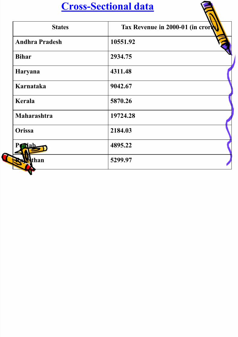
• In cross-section data, values of one or morevariables are collected for several sample units,or entities at the same point in time (e.g. GDPfigure of countries for a given year).
C S ti l d t
8/21/2019 Application of Econometrics in Economics
http://slidepdf.com/reader/full/application-of-econometrics-in-economics 23/160
Cross-Sectional data
States Tax Revenue in 2000-01 (in crores)
Andhra Pradesh 10551.92
Bihar 2934.75
Haryana 4311.48
Karnataka 9042.67
Kerala 5870.26
Maharashtra 19724.28
Orissa 2184.03
Punjab 4895.22
Rajasthan 5299.97
8/21/2019 Application of Econometrics in Economics
http://slidepdf.com/reader/full/application-of-econometrics-in-economics 24/160
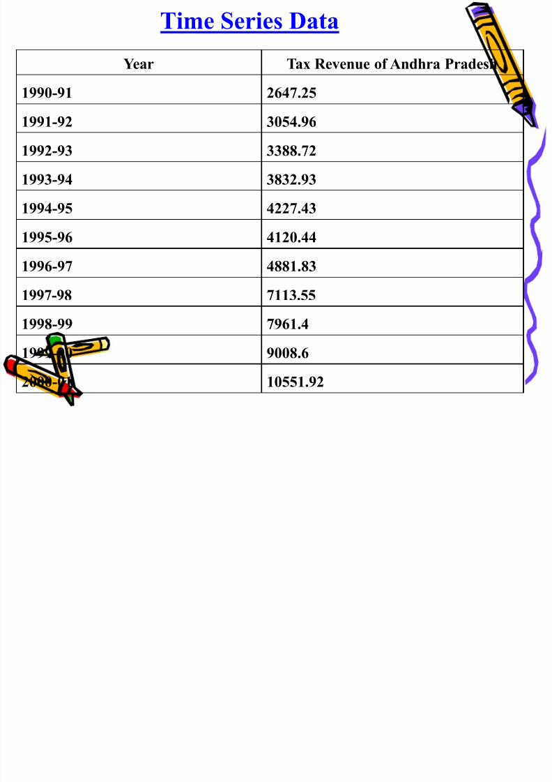
• In time series data we observe the values of oneor more variables over a period of time – daily
stock prices or annual GDP figures
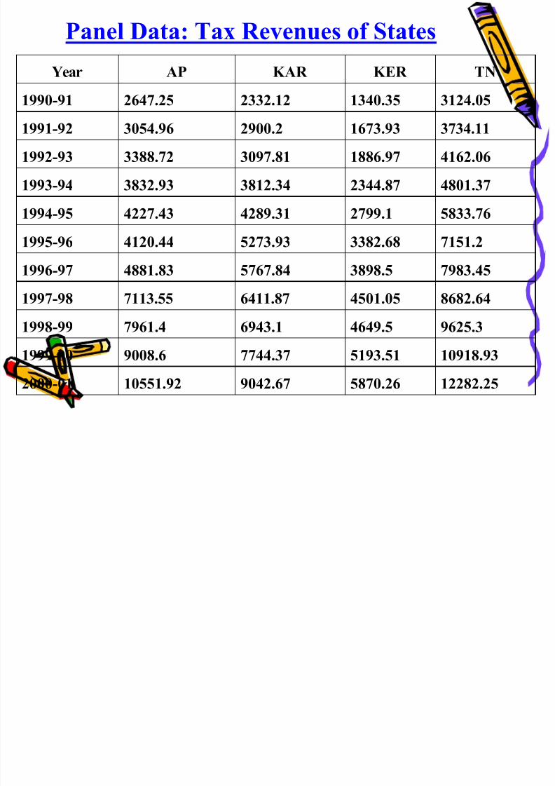
• In panel data, same cross-sectional unit (say afirm or state or country) is surveyed over time
• Thus, in panel data we have elements of bothtime series and cross-sectional data.
8/21/2019 Application of Econometrics in Economics
http://slidepdf.com/reader/full/application-of-econometrics-in-economics 25/160
Time Series Data
Year Tax Revenue of Andhra Pradesh
1990-91 2647.25
1991-92 3054.96
1992-93 3388.72
1993-94 3832.93
1994-95 4227.43
1995-96 4120.44
1996-97 4881.83
1997-98 7113.55
1998-99 7961.4
1999-00 9008.6
2000-01 10551.92
8/21/2019 Application of Econometrics in Economics
http://slidepdf.com/reader/full/application-of-econometrics-in-economics 26/160
Panel Data: Tax Revenues of States
Year AP KAR KER TN 1990-91 2647.25 2332.12 1340.35 3124.05 1991-92 3054.96 2900.2 1673.93 3734.11 1992-93 3388.72 3097.81 1886.97 4162.06 1993-94 3832.93 3812.34 2344.87 4801.37 1994-95 4227.43 4289.31 2799.1 5833.76 1995-96 4120.44 5273.93 3382.68 7151.2 1996-97 4881.83 5767.84 3898.5 7983.45 1997-98 7113.55 6411.87 4501.05 8682.64 1998-99 7961.4 6943.1 4649.5 9625.3 1999-00 9008.6 7744.37 5193.51 10918.93 2000-01
10551.92
9042.67
5870.26
12282.25
8/21/2019 Application of Econometrics in Economics
http://slidepdf.com/reader/full/application-of-econometrics-in-economics 27/160
Step 4: Specify Econometric Model
• LFPR = B1 + B2UR +u
LFPR – Labour force participation rate
UR – Unemployment rate (a proxy for economic
condition. Other option could be GDP)
B 1 - Intercept term. Gives value of LFPR (dependent
variable) when UR (value of independent variable) iszero
8/21/2019 Application of Econometrics in Economics
http://slidepdf.com/reader/full/application-of-econometrics-in-economics 28/160
B 2 - Slope term. Measures the rate of change in LFPR
for a unit change in UR. Together B1 and B2 are
known as the parameters of the regression modelu – Error term [LFPR – ( B1 + B2UR)]
• This is a linear regression model - LFPR is linearly
related to UR
• Our objective is to explain the behaviour of dependent
variable in relation to the explanatory variable.
8/21/2019 Application of Econometrics in Economics
http://slidepdf.com/reader/full/application-of-econometrics-in-economics 29/160
Step 5: Data Collection
• For empirical estimation, we need to collect dataon the variables used in the econometric model.
• Data can be obtained either from primary sources[HR] or from secondary sources [Finance,
Economics]
8/21/2019 Application of Econometrics in Economics
http://slidepdf.com/reader/full/application-of-econometrics-in-economics 30/160
Step 6: Model Estimation
• By estimation we mean estimating the parameters(B1 & B2) of the chosen model.
• Estimation is carried out using the technique of
regression analysis.
8/21/2019 Application of Econometrics in Economics
http://slidepdf.com/reader/full/application-of-econometrics-in-economics 31/160
• What is regression analysis?
“Regression analysis is concerned with thestudy of the dependence of one variable, the
dependent variable, on one or more other
variables, the explanatory var iables, with a view
to estimating and/or predicting the (population)
mean or average value of the former in terms of
the known or fixed (in repeated sampling)
values of the latter ”
8/21/2019 Application of Econometrics in Economics
http://slidepdf.com/reader/full/application-of-econometrics-in-economics 32/160
• Assume that after estimation we get the followingresult:
LFPR = 50.63 - 0.45UR
B2 = – 0.45. Implies that if UR goes up by 1%
point, ceteris paribus, LFPR is expected todecrease on the average by about 0.45% points – Discouraged worker hypothesis finds support.
B1 = 50.63. Implies that average value of LFRPwill be about 50.63% if the UR were zero (i.e.full employment).
8/21/2019 Application of Econometrics in Economics
http://slidepdf.com/reader/full/application-of-econometrics-in-economics 33/160
Sometimes/often, intercept term has no
particular economic meaning.
But, in the present example it has meaning
(How?)
We say “on the average” because the presence
of error term is likely to make the relationship
somewhat imprecise.
8/21/2019 Application of Econometrics in Economics
http://slidepdf.com/reader/full/application-of-econometrics-in-economics 34/160
Step 7: Hypothesis Testing
• Objective here is to test certain hypothesessuggested by theory and/or prior empirical
experience on parameters of the model.
• Specifically, we are interested to verify how
close the estimated parameter is to a pre-
supposed value of that parameter
(e.g. )45.0ˆ;1: 110 B B H
8/21/2019 Application of Econometrics in Economics
http://slidepdf.com/reader/full/application-of-econometrics-in-economics 35/160
• Hypothesis testing helps to verify whether the
results obtained through regression analysis
conform to the underlying theory
8/21/2019 Application of Econometrics in Economics
http://slidepdf.com/reader/full/application-of-econometrics-in-economics 36/160
Step 8: Using Estimated Model for
Forecasting/Prediction
• LFPR = 50.6333 - 0.4486UR
• If we want to predict LFPR in some future
periods for a given value of UR (say 5) we can
obtain it (How?)
• Substitute UR value (5) in the above equation
8/21/2019 Application of Econometrics in Economics
http://slidepdf.com/reader/full/application-of-econometrics-in-economics 37/160
• When data on LFPR (for a given UR ) for
future period is out, we can compare the
predicted value with the actual value.
• The discrepancy between the two is called the
prediction error.
8/21/2019 Application of Econometrics in Economics
http://slidepdf.com/reader/full/application-of-econometrics-in-economics 38/160
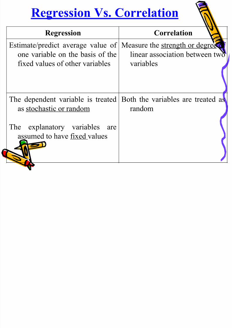
Regression Vs. Correlation
Regression Correlation
Estimate/predict average value of
one variable on the basis of the
fixed values of other variables
Measure the strength or degree of
linear association between two
variables
The dependent variable is treated
as stochastic or random
The explanatory variables are
assumed to have fixed values
Both the variables are treated as
random
O I di t T k
8/21/2019 Application of Econometrics in Economics
http://slidepdf.com/reader/full/application-of-econometrics-in-economics 39/160
Our Immediate Task
• Identification of research issue, selection of
variables, checking of data availability,specification of econometric model and data
collection are not big tasks
• Hence, our focus would be on
Model Estimation
Hypothesis Testing
8/21/2019 Application of Econometrics in Economics
http://slidepdf.com/reader/full/application-of-econometrics-in-economics 40/160
Criticisms
• By and large, events can be explained without
econometric analysis
• Data mining – Results are created!
• Problem with intercept term
8/21/2019 Application of Econometrics in Economics
http://slidepdf.com/reader/full/application-of-econometrics-in-economics 41/160
Two-Variable Regression Model
8/21/2019 Application of Econometrics in Economics
http://slidepdf.com/reader/full/application-of-econometrics-in-economics 42/160
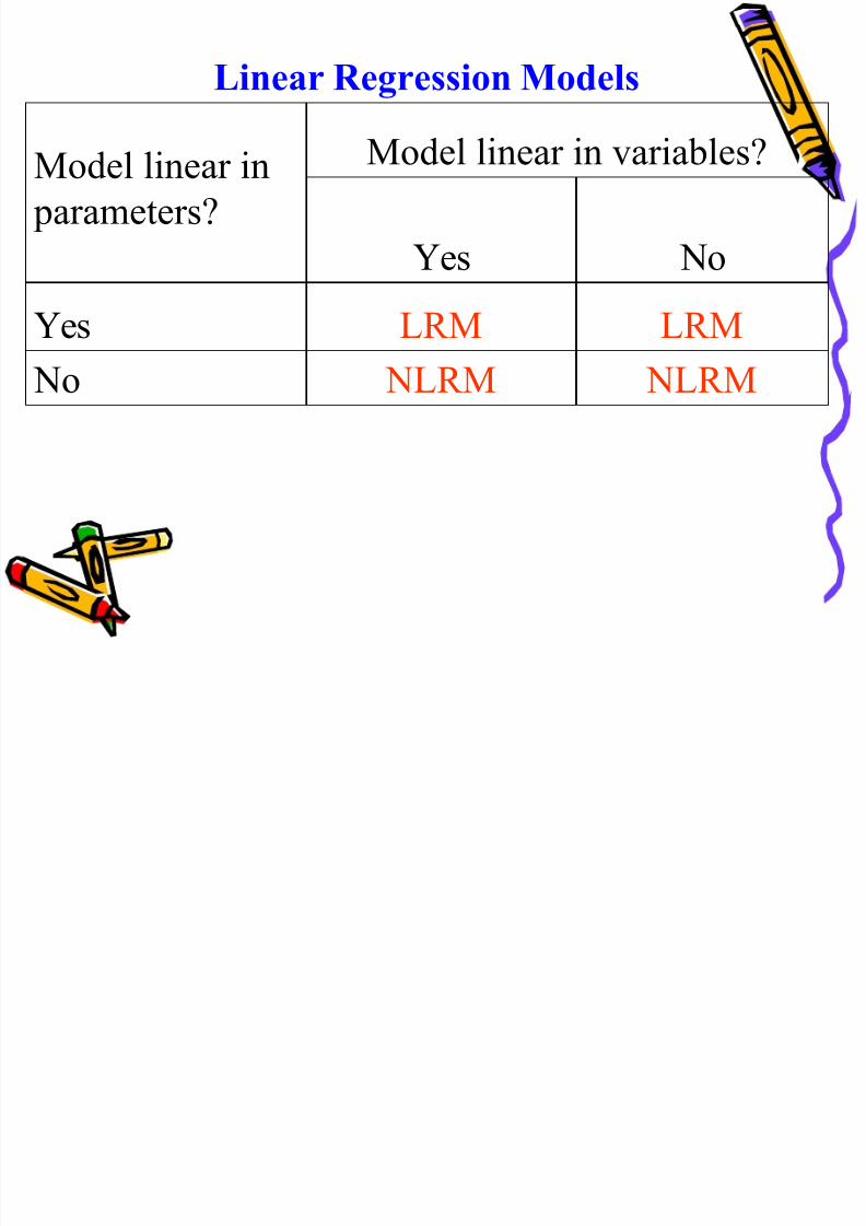
• Term linear can be interpreted in 2 ways:
Linearity in the variables and linearity in the parameters.
• “Linear” regression always means a regressionthat is linear in the parameters. It may or may not
be linear in the explanatory variables
Example:Y = B1 + B2X +u (or)
Y = B1 + B2X2 +u
8/21/2019 Application of Econometrics in Economics
http://slidepdf.com/reader/full/application-of-econometrics-in-economics 43/160
Linear Regression Models
Model linear in parameters?
Model linear in variables?
Yes No
Yes LRM LRM
No NLRM NLRM
P l ti R i F ti (PRF)
8/21/2019 Application of Econometrics in Economics
http://slidepdf.com/reader/full/application-of-econometrics-in-economics 44/160
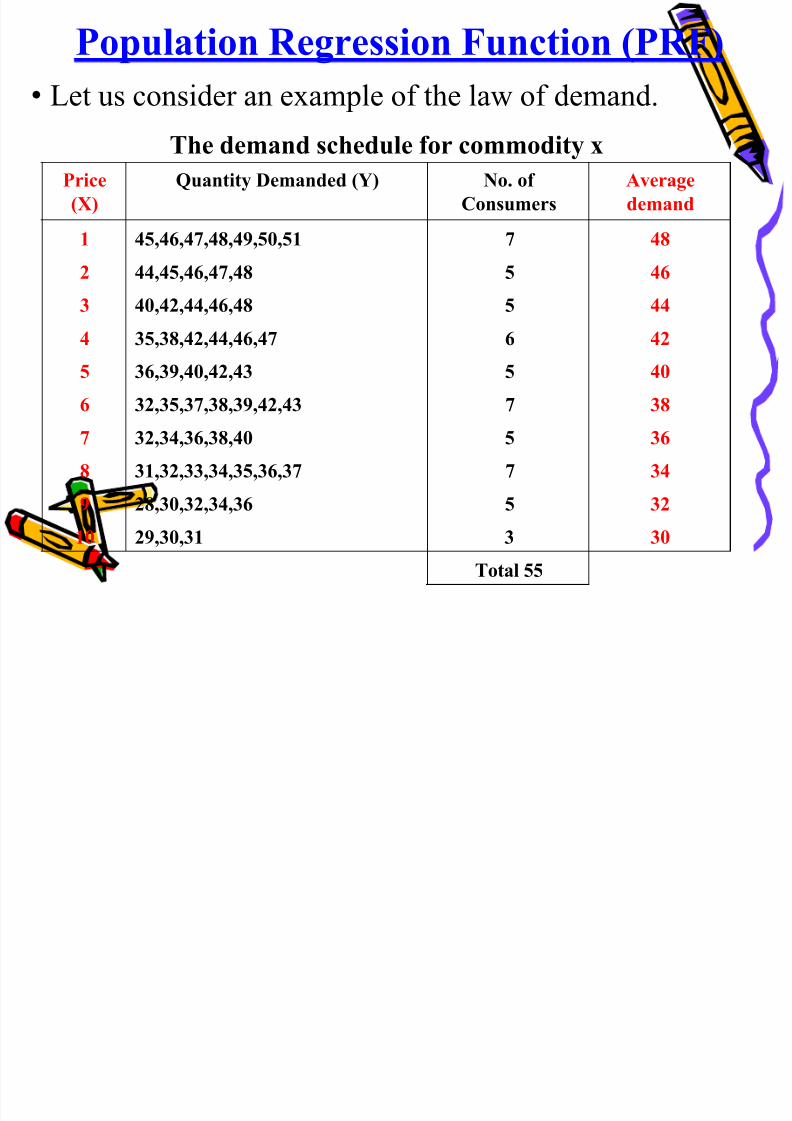
Population Regression Function (PRF)
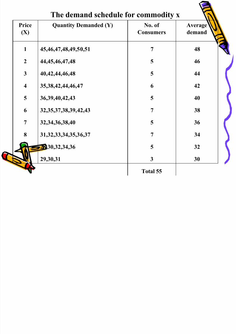
• Let us consider an example of the law of demand.
The demand schedule for commodity x Price
(X)
Quantity Demanded (Y) No. of
Consumers
Average
demand
1 45,46,47,48,49,50,51 7 48
2 44,45,46,47,48 5 46
3 40,42,44,46,48 5 44
4 35,38,42,44,46,47 6 42
5 36,39,40,42,43 5 40
6 32,35,37,38,39,42,43 7 38
7 32,34,36,38,40 5 36
8 31,32,33,34,35,36,37 7 34
9 28,30,32,34,36 5 32
10 29,30,31 3 30
Total 55
8/21/2019 Application of Econometrics in Economics
http://slidepdf.com/reader/full/application-of-econometrics-in-economics 45/160
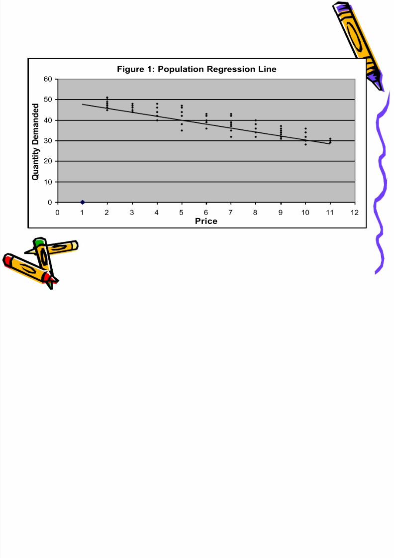
Figure 1: Population Regression Line
0
10
20
30
40
50
60
0 1 2 3 4 5 6 7 8 9 10 11 12
Price
Q u a n t i t y D e m a n d e d
8/21/2019 Application of Econometrics in Economics
http://slidepdf.com/reader/full/application-of-econometrics-in-economics 46/160
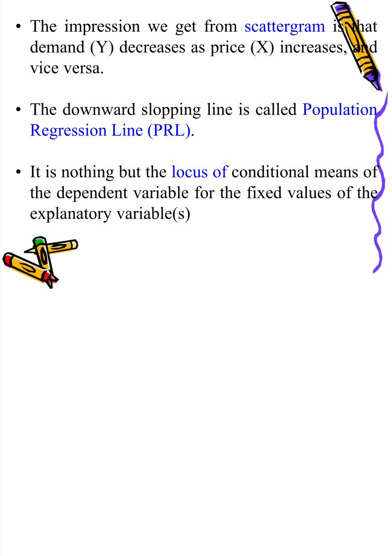
• The impression we get from scattergram is that
demand (Y) decreases as price (X) increases, and
vice versa.
• The downward slopping line is called Population
Regression Line (PRL).
• It is nothing but the locus of conditional means of
the dependent variable for the fixed values of the
explanatory variable(s)
8/21/2019 Application of Econometrics in Economics
http://slidepdf.com/reader/full/application-of-econometrics-in-economics 47/160
• Thus, PRL gives the average value of the
dependent variable corresponding to each value
of the independent variable.
• The point on the PRL represents expected or
population mean value of Y corresponding to
the various Xs.
• The adjective population comes as our example
deals with entire population of 55 consumers.
8/21/2019 Application of Econometrics in Economics
http://slidepdf.com/reader/full/application-of-econometrics-in-economics 48/160
• PRL can be expressed in following functional
form:
E(Y/Xi) = B1+B2Xi (1)
where i is ith subpopulation
• Eq (1) gives average value of Y corresponding to
each value of X and is called Population
Regression Function (PRF) or non-stochastic
PRF.
8/21/2019 Application of Econometrics in Economics
http://slidepdf.com/reader/full/application-of-econometrics-in-economics 49/160
• In regression analysis our interest is in
estimating the PRFs (i.e. B1 and B2) on the basis
of observations on Y and X.
8/21/2019 Application of Econometrics in Economics
http://slidepdf.com/reader/full/application-of-econometrics-in-economics 50/160
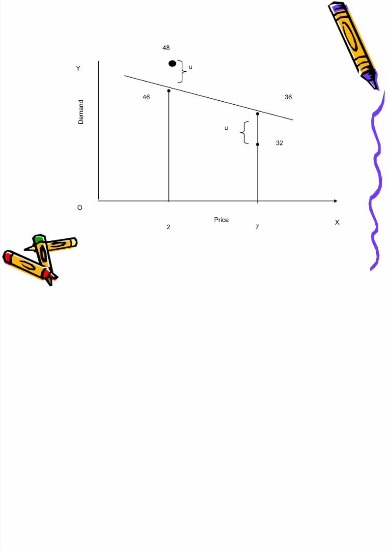
Stochastic Specification of the PRF
• How to explain the demands of the individualconsumer in relation to price?
• The best we can do is to say that any
individual‟s demand is equal to the average for
that group plus or minus some quantity.
8/21/2019 Application of Econometrics in Economics
http://slidepdf.com/reader/full/application-of-econometrics-in-economics 51/160
D e m a n d
O
2 7X
36
u
32
Price
u
46
Y
48
8/21/2019 Application of Econometrics in Economics
http://slidepdf.com/reader/full/application-of-econometrics-in-economics 52/160
• We can express the deviation of an individual Yi
around its expected value as follows:
Yi = E(Y/Xi) + ui (2)
• In Eq. (2), ui is an unobservable random variable
– called stochastic error term - taking positive or
negative values.
8/21/2019 Application of Econometrics in Economics
http://slidepdf.com/reader/full/application-of-econometrics-in-economics 53/160
• Now, by substituting Eq. (1) in (2), we get
Yi = B1+B2Xi+ui (3)
• Eq. (3) is called stochastic PRF (SPRF), whereas
Eq. (1) is called non-stochastic PRF (NPRF).
• NPRF represents means of various Y values
corresponding to specified prices.
• SPRF tells us how individual demands vary around
their mean values due to presence of stochastic error
term, u .
8/21/2019 Application of Econometrics in Economics
http://slidepdf.com/reader/full/application-of-econometrics-in-economics 54/160
• How to interpret SPRF (Eq.3)?
• We can say that demand of an individual consumer
(say i) corresponding to a specific price can be
expressed as sum of following 2 components:
(i) Systematic/deterministic component:
B1+B2Xi (Nothing but average quantity demanded
by all the consumers at a given price level Xi)
8/21/2019 Application of Econometrics in Economics
http://slidepdf.com/reader/full/application-of-econometrics-in-economics 55/160
(ii) Nonsystematic/random component: ui
(Determined by factors other than price) [See
Figure]

8/21/2019 Application of Econometrics in Economics
http://slidepdf.com/reader/full/application-of-econometrics-in-economics 56/160
D e m a n d
O
2 7X
36
u
32
Price
u
46
Y
48
8/21/2019 Application of Econometrics in Economics
http://slidepdf.com/reader/full/application-of-econometrics-in-economics 57/160
Sample Regression Function (SRF)
• If we have data on whole population (like in
following Table) arriving at PRF is an
easy/straightforward exercise
• That is, find conditional means of Ycorresponding to each X and then join these
means
• Unfortunately, in practice, we rarely have entire population at our disposal.
Th d d h d l f di
8/21/2019 Application of Econometrics in Economics
http://slidepdf.com/reader/full/application-of-econometrics-in-economics 58/160
The demand schedule for commodity x
Price
(X)
Quantity Demanded (Y) No. of
Consumers
Average
demand
1 45,46,47,48,49,50,51 7 48
2 44,45,46,47,48 5 46
3 40,42,44,46,48 5 44
4 35,38,42,44,46,47 6 42
5 36,39,40,42,43 5 40
6 32,35,37,38,39,42,43 7 38
7 32,34,36,38,40 5 36
8 31,32,33,34,35,36,37 7 34
9 28,30,32,34,36 5 32
10 29,30,31 3 30
Total 55
W l h l f h l i

8/21/2019 Application of Econometrics in Economics
http://slidepdf.com/reader/full/application-of-econometrics-in-economics 59/160
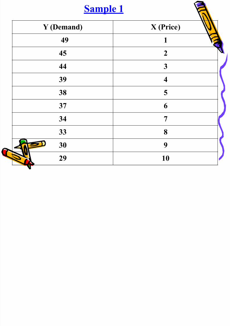
• We only have a sample from the population.
• The following is an example from our case
Sample 1
8/21/2019 Application of Econometrics in Economics
http://slidepdf.com/reader/full/application-of-econometrics-in-economics 60/160
p
Y (Demand) X (Price)
49 145 2
44 3
39 438 5
37 6
34 7
33 8
30 9
29 10
H t k i t ti t th PRF th b i f
8/21/2019 Application of Econometrics in Economics
http://slidepdf.com/reader/full/application-of-econometrics-in-economics 61/160
• Hence, our task is to estimate the PRF on the basis of
sample information
[OR]
Task is to estimate average quantity demanded in the
population as a whole corresponding to each X (price)from sample data such as above
• But, we may not be able to estimate the PRF accurately
because of sampling error
8/21/2019 Application of Econometrics in Economics
http://slidepdf.com/reader/full/application-of-econometrics-in-economics 62/160
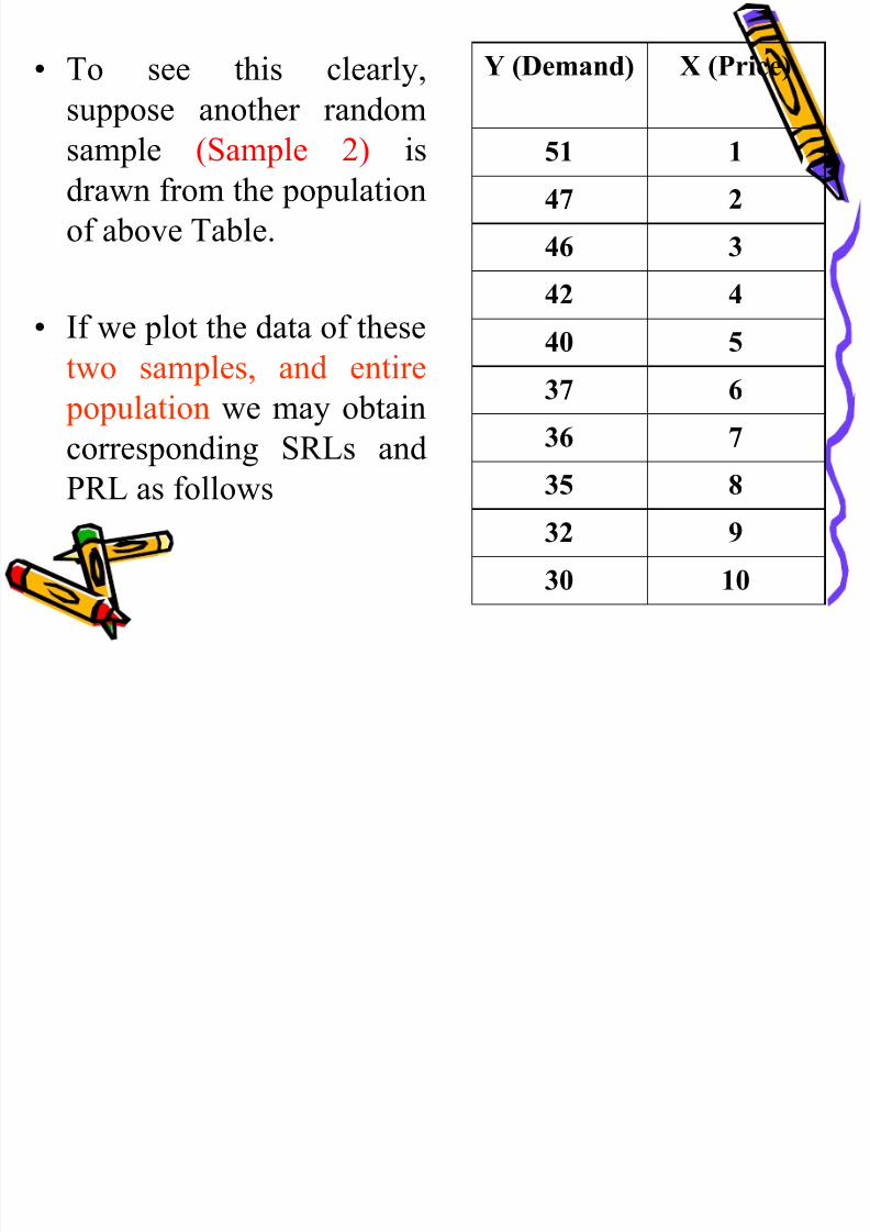
• To see this clearly,
suppose another random
sample (Sample 2) isdrawn from the population
of above Table.
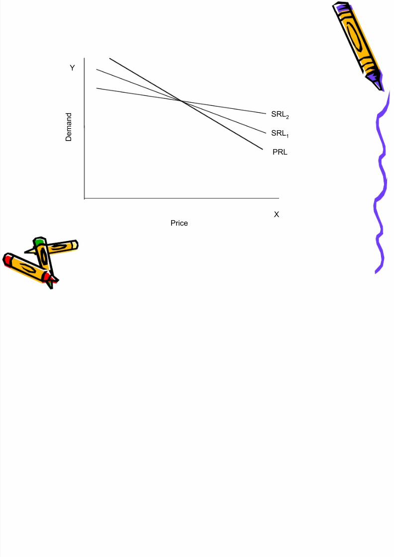
• If we plot the data of these
two samples, and entire
population we may obtain
corresponding SRLs and
PRL as follows
Y (Demand) X (Price)
51
1
47 2
46 3
42 4
40 5
37 6
36 7
35 8
32 9
30 10
8/21/2019 Application of Econometrics in Economics
http://slidepdf.com/reader/full/application-of-econometrics-in-economics 63/160
D e m a n d
Y
X
SRL1
SRL2
PRL
Price
N th ti i hi h f th t SRL
8/21/2019 Application of Econometrics in Economics
http://slidepdf.com/reader/full/application-of-econometrics-in-economics 64/160
• Now the question is: which of the two SRLs
represents the “true” PRL?
• If we avoid temptation of looking at above
figure, which represents the PRL, there is no way
we can be sure that either of the SRLs represents
the true PRL
• In general, we get K different SRLs for K
different samples and all these SRLs are notlikely to be the same
N l t PRF th t d li th PRL

8/21/2019 Application of Econometrics in Economics
http://slidepdf.com/reader/full/application-of-econometrics-in-economics 65/160
• Now, analogous to PRF that underlies the PRL,
we can develop SRF to represent SRL as
follows:
= estimator of E(Y/Xi) b1 = estimator of B1
b2 = estimator of B2
Where is read as “Y-hat” or “Y-cap” Y
)4(ˆ21 ii
X bbY
iY ˆ
A ti t i l f l th t i di t
8/21/2019 Application of Econometrics in Economics
http://slidepdf.com/reader/full/application-of-econometrics-in-economics 66/160
• An estimator is a rule or formula that indicates
how to estimate the population parameter at
hand.
• A particular numerical value obtained by the
estimator is an estimate.
• Now, we can express SRF (Eq.4) in its
stochastic form as follows:
b + b X + e (5)Y
8/21/2019 Application of Econometrics in Economics
http://slidepdf.com/reader/full/application-of-econometrics-in-economics 67/160
= b1 + b2Xi + ei (5)
Where ei is the estimator of ui
• It is analogous to ui and is introduced for same
reasons as ui was introduced in the PRF
iY
T i bj i i i
8/21/2019 Application of Econometrics in Economics
http://slidepdf.com/reader/full/application-of-econometrics-in-economics 68/160
• To sum up, our primary objective in regression
analysis is to estimate the stochastic PRF (Eq.3)
on the basis of stochastic SRF (Eq.5) becausemore often than not our analysis is based on a
single sample from some population.
• But, because of sampling variation, our estimate
of PRF based on SRF is only approximate.
8/21/2019 Application of Econometrics in Economics
http://slidepdf.com/reader/full/application-of-econometrics-in-economics 69/160
D e m a n d
Y
X
PRF
SRF
Price
Error
Error
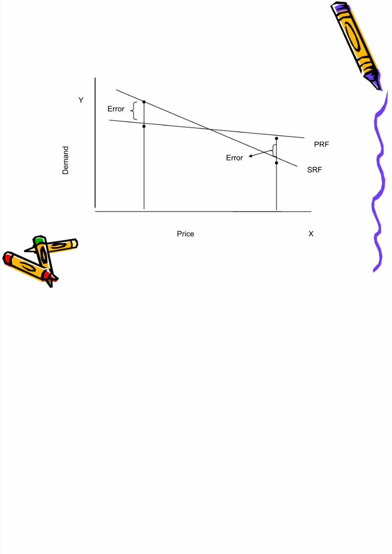
• Granted that SRF is only an approximation of the PRF

8/21/2019 Application of Econometrics in Economics
http://slidepdf.com/reader/full/application-of-econometrics-in-economics 70/160
• Granted that SRF is only an approximation of the PRF
the question is:
• Can we find a method or a procedure that will make
this approximation as “close” as possible?
[OR]
How should we construct the SRF so that b1 is as close
as possible to B1 and b2 is as close as possible to B2?
• This can be done by adopting the method of Ordinary
Least Squares (OLS).
What is OLS method?
8/21/2019 Application of Econometrics in Economics
http://slidepdf.com/reader/full/application-of-econometrics-in-economics 71/160
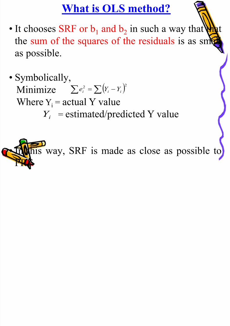
• It chooses SRF or b1 and b2 in such a way that that
the sum of the squares of the residuals is as smallas possible.
• Symbolically,
Minimize
Where Yi = actual Y value
= estimated/predicted Y value
• In this way, SRF is made as close as possible to
PRF
2
2 ˆiii Y Y e
iY ˆ
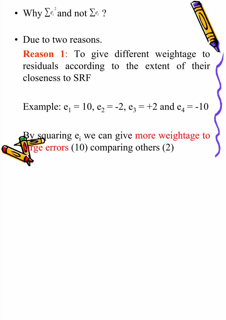
• Why and not ?2
ie ie
8/21/2019 Application of Econometrics in Economics
http://slidepdf.com/reader/full/application-of-econometrics-in-economics 72/160
Why and not ?
• Due to two reasons. Reason 1: To give different weightage to
residuals according to the extent of their
closeness to SRF
Example: e1 = 10, e2 = -2, e3 = +2 and e4 = -10
By squaring ei we can give more weightage to
large errors (10) comparing others (2)
i i
R 2 Thi d id th bl f

8/21/2019 Application of Econometrics in Economics
http://slidepdf.com/reader/full/application-of-econometrics-in-economics 73/160
Reason 2: This procedure avoids the problem of
sign of the residuals which can be positive as
well as negative, and therefore can add to zero.
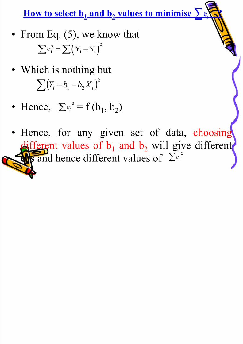
How to select b1 and b2 values to minimise ?2
ie
8/21/2019 Application of Econometrics in Economics
http://slidepdf.com/reader/full/application-of-econometrics-in-economics 74/160
ow to se ect b1 a d b2 va ues to se ?ie
• From Eq. (5), we know that
• Which is nothing but
• Hence, = f (b1, b2)
• Hence, for any given set of data, choosingdifferent values of b1 and b2 will give different
ei‟s and hence different values of
22
i i iˆe Y Y
2
21 ii X bbY
2
ie
2
ie
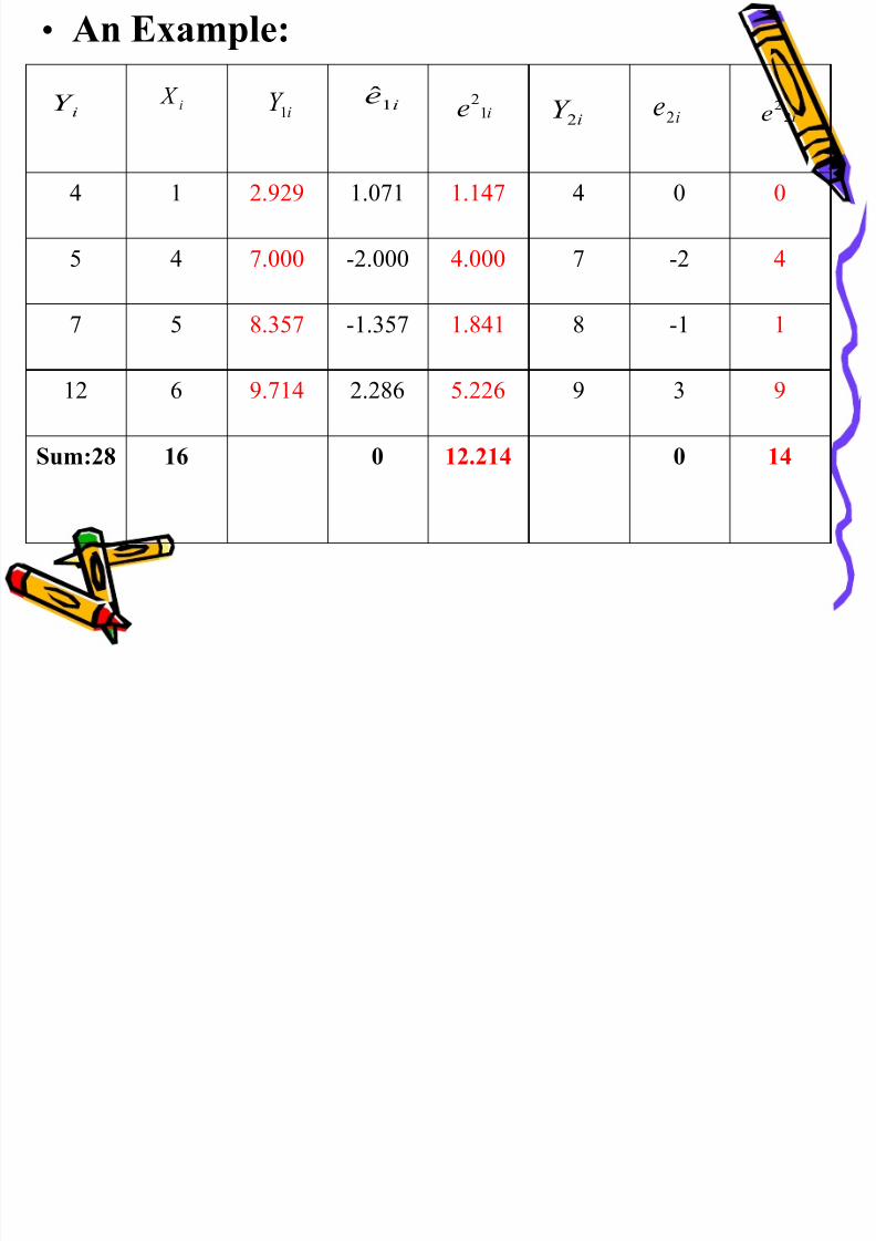
• An Example:
8/21/2019 Application of Econometrics in Economics
http://slidepdf.com/reader/full/application-of-econometrics-in-economics 75/160
4 1 2.929 1.071 1.147 4 0 0
5 4 7.000 -2.000 4.000 7 -2 4
7 5 8.357 -1.357 1.841 8 -1 1
12 6 9.714 2.286 5.226 9 3 9
Sum:28 16 0 12.214 0 14
iY i X iY 1
ˆ ie1ˆ
ie 12
ˆiY 2
ˆie2
ˆie 2
2ˆ
ˆ
8/21/2019 Application of Econometrics in Economics
http://slidepdf.com/reader/full/application-of-econometrics-in-economics 76/160
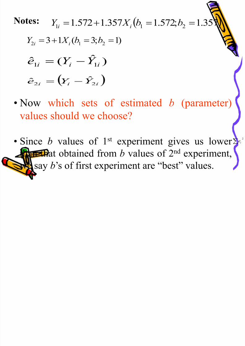
Notes:
• Now which sets of estimated b (parameter)
values should we choose?
• Since b values of 1st experiment gives us lower
than that obtained from b values of 2nd experiment,
we say b‟s of first experiment are “best” values.
357.1;572.1357.1572.1ˆ211
bb X Y ii
)1;3(13ˆ212 bb X Y ii
)ˆ(ˆ 11 iii Y Y e
iii Y Y e 22
ˆˆ
2
ie
B h d i hi ?

8/21/2019 Application of Econometrics in Economics
http://slidepdf.com/reader/full/application-of-econometrics-in-economics 77/160
• But how do we ascertain this?
• We still can choose many more values for b‟s that gives us the least possible value of
• However, in doing so we must be sure that we
have considered all the conceivable values of b1 and b2
• If we have infinite time and patience we can do
this exercise
2
ie
• But fortunately OLS method chooses b and b
8/21/2019 Application of Econometrics in Economics
http://slidepdf.com/reader/full/application-of-econometrics-in-economics 78/160
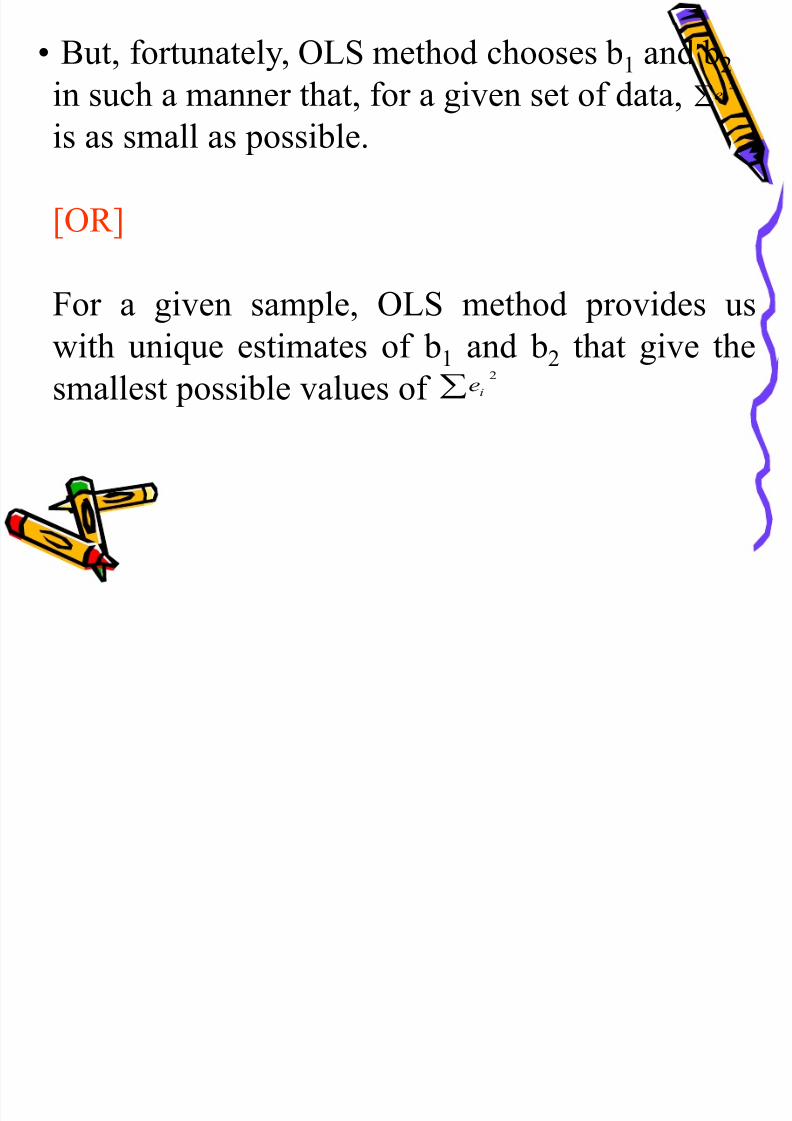
• But, fortunately, OLS method chooses b1 and b2
in such a manner that, for a given set of data,
is as small as possible.
[OR]
For a given sample, OLS method provides us
with unique estimates of b1 and b2 that give the
smallest possible values of
2
ie
2
ie
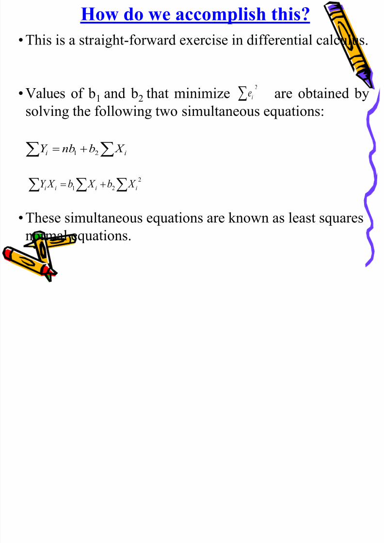
How do we accomplish this?
8/21/2019 Application of Econometrics in Economics
http://slidepdf.com/reader/full/application-of-econometrics-in-economics 79/160
• This is a straight-forward exercise in differential calculus.
• Values of b1 and b2 that minimize are obtained by
solving the following two simultaneous equations:
• These simultaneous equations are known as least squares
normal equations.
2
ie
ii X bnbY 21
2
21 iiii X b X b X Y
• In above equations n is sample size
8/21/2019 Application of Econometrics in Economics
http://slidepdf.com/reader/full/application-of-econometrics-in-economics 80/160
• In above equations n is sample size
• Unknowns are bs. Knowns are quantities
involving sums, sum of squares, and sums of
cross products of the variables Y and X
• The knowns can be obtained from sample athand
• Solving these equations simultaneously, we
obtain following solutions for b1 and b2:
8/21/2019 Application of Econometrics in Economics
http://slidepdf.com/reader/full/application-of-econometrics-in-economics 81/160
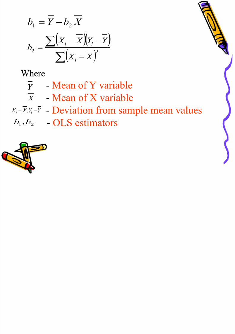
Where
- Mean of Y variable- Mean of X variable
- Deviation from sample mean values
- OLS estimators
X bY b 21
22
X X
Y Y X X b
i
ii
Y X
Y Y X X ii ,
21,bb
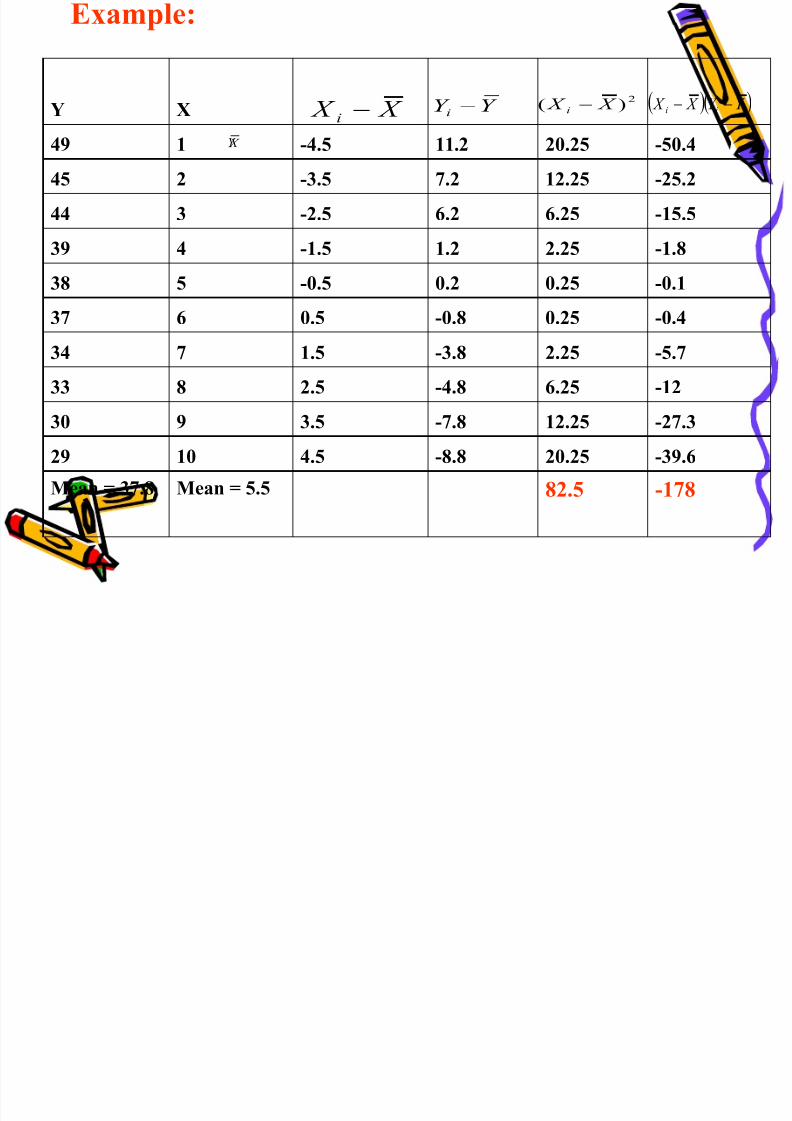
Example:
8/21/2019 Application of Econometrics in Economics
http://slidepdf.com/reader/full/application-of-econometrics-in-economics 82/160
Y X
Y X
49
1
-4.5
11.2
20.25
-50.4
45 2 -3.5 7.2 12.25 -25.2
44 3 -2.5 6.2 6.25 -15.5
39 4 -1.5 1.2 2.25 -1.8
38
5
-0.5
0.2
0.25
-0.1
37 6 0.5 -0.8 0.25 -0.4
34 7 1.5 -3.8 2.25 -5.7
33 8 2.5 -4.8 6.25 -12
30 9 3.5 -7.8 12.25 -27.3 29 10 4.5 -8.8 20.25 -39.6
Mean = 37.8 Mean = 5.5 82.5 -178
X X i Y Y i
2)( X X i Y Y X X ii
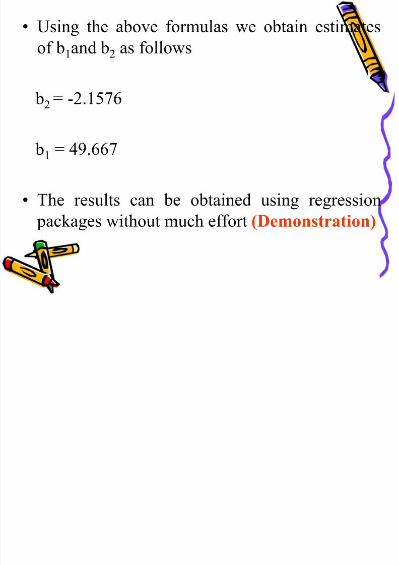
• Using the above formulas we obtain estimates
8/21/2019 Application of Econometrics in Economics
http://slidepdf.com/reader/full/application-of-econometrics-in-economics 83/160
Using the above formulas we obtain estimates
of b1and b2 as follows
b2 = -2.1576
b1 = 49.667
• The results can be obtained using regression
packages without much effort (Demonstration)
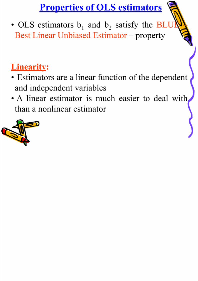
Properties of OLS estimators
8/21/2019 Application of Econometrics in Economics
http://slidepdf.com/reader/full/application-of-econometrics-in-economics 84/160
• OLS estimators b1 and b2 satisfy the BLUE –
Best Linear Unbiased Estimator – property
Linearity:
• Estimators are a linear function of the dependent
and independent variables
• A linear estimator is much easier to deal with
than a nonlinear estimator
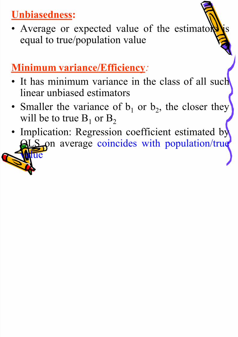
Unbiasedness:
8/21/2019 Application of Econometrics in Economics
http://slidepdf.com/reader/full/application-of-econometrics-in-economics 85/160
• Average or expected value of the estimators isequal to true/population value
Minimum variance/Efficiency:
• It has minimum variance in the class of all suchlinear unbiased estimators
• Smaller the variance of b1 or b2, the closer theywill be to true B1 or B2
• Implication: Regression coefficient estimated byOLS on average coincides with population/truevalue
Assumptions Underlying OLS
8/21/2019 Application of Econometrics in Economics
http://slidepdf.com/reader/full/application-of-econometrics-in-economics 86/160
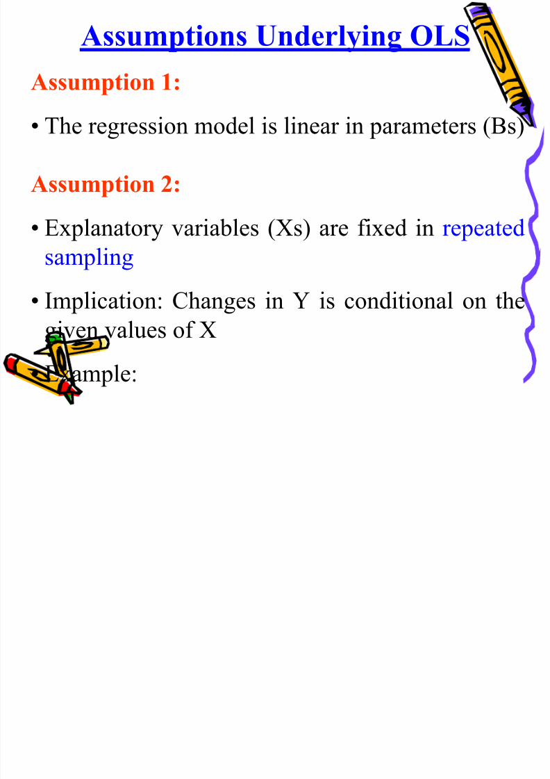
Assumptions Underlying OLS
Assumption 1:
• The regression model is linear in parameters (Bs)
Assumption 2:
• Explanatory variables (Xs) are fixed in repeated
sampling
• Implication: Changes in Y is conditional on thegiven values of X
• Example:
The demand schedule for commodity x
8/21/2019 Application of Econometrics in Economics
http://slidepdf.com/reader/full/application-of-econometrics-in-economics 87/160
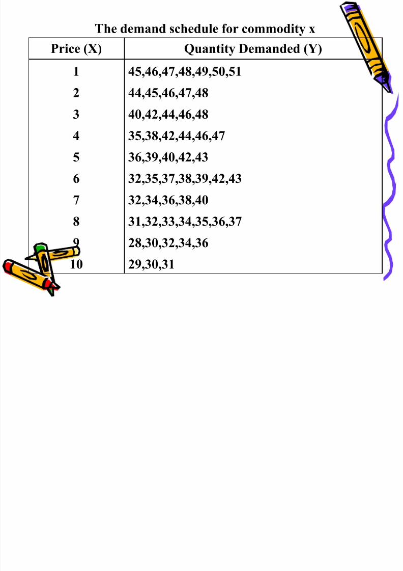
The demand schedule for commodity x
Price (X) Quantity Demanded (Y)
1
45,46,47,48,49,50,51
2 44,45,46,47,48
3 40,42,44,46,48
4 35,38,42,44,46,47
5 36,39,40,42,43
6 32,35,37,38,39,42,43
7 32,34,36,38,40
8 31,32,33,34,35,36,37
9 28,30,32,34,36
10 29,30,31
Assumption 3:
8/21/2019 Application of Econometrics in Economics
http://slidepdf.com/reader/full/application-of-econometrics-in-economics 88/160
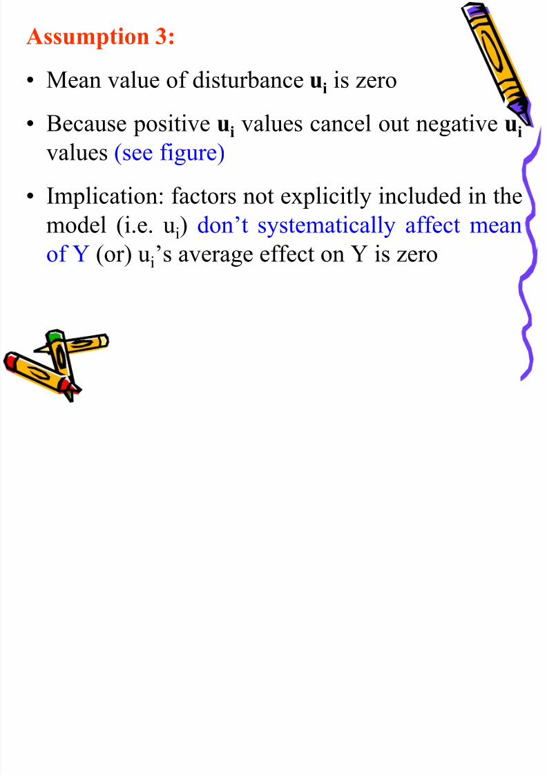
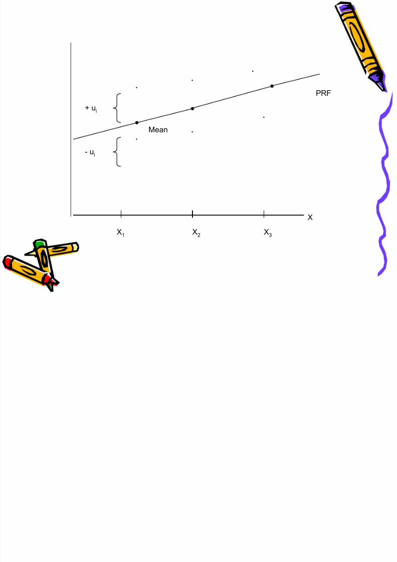
Assumption 3:
• Mean value of disturbance ui is zero
• Because positive ui values cancel out negative ui
values (see figure)
• Implication: factors not explicitly included in themodel (i.e. ui) don‟t systematically affect mean
of Y (or) ui‟s average effect on Y is zero
8/21/2019 Application of Econometrics in Economics
http://slidepdf.com/reader/full/application-of-econometrics-in-economics 89/160
X
X1 X2 X3
PRF
+ ui
- ui
Mean
. .
. .
.
.
Assumption 4:
8/21/2019 Application of Econometrics in Economics
http://slidepdf.com/reader/full/application-of-econometrics-in-economics 90/160
p
• The variance of ui is same for all observations
(Xs) [Homoscedasticity or equal (homo) spread
(scedasticity)]
• Implication: Variation around regression line ofindividual Y values remains same regardless of
values taken by Xs; it neither increases or
decreases as X varies
• Hence all Y values corresponding to the various
Xs are equally important.
• Violation of this assumption (i.e. increase in variation
8/21/2019 Application of Econometrics in Economics
http://slidepdf.com/reader/full/application-of-econometrics-in-economics 91/160
around regression line of Y values as X increases) is
called heteroscedasticity
• Example for homoscedasticity: Richer families on
average consume more than poorer families, but there
is no/not much variability in consumption pattern between richer and poorer families
• Example for heteroscedasticity: There is greater
variability in consumption pattern of richer families
compared to poorer ones becoz. as income grows
people have more consumption choice.
Assumption 5:
8/21/2019 Application of Econometrics in Economics
http://slidepdf.com/reader/full/application-of-econometrics-in-economics 92/160
• No autocorrelation between error terms
(Implications for time series data)
• Example for autocorrelation:Yt = B1 +B2Xt +ut, where ut and ut-1 are positively
correlated. Here, Yt depends not only on Xt, but
also on ut-1 for ut-1 to some extent determined ut
• By invoking no autocorrelation assumption, we
8/21/2019 Application of Econometrics in Economics
http://slidepdf.com/reader/full/application-of-econometrics-in-economics 93/160
y g p ,
consider only the effect on Xt on Yt and not
worry about other influences that might act on Yas a result of possible inter-correlations among
u‟s
Assumption 6:
8/21/2019 Application of Econometrics in Economics
http://slidepdf.com/reader/full/application-of-econometrics-in-economics 94/160
Assumption 6:
• No correlation between u and explanatory
variables (Xs)
• Implication: If X and u are correlated, it is not
possible to assess their individual effects on Y
• If X and u are positively correlated, X increases
when u increases and it decreases when u
decreases.
Assumption 7:
8/21/2019 Application of Econometrics in Economics
http://slidepdf.com/reader/full/application-of-econometrics-in-economics 95/160
• Number of observations n must be greater than the
number of parameters to be estimated or explanatory
variables.
Assumption 8:
• X values in given sample must not all be the same(Applies to Y as well)
• If so, Xi = and hence denominator of estimator b2
will be zero.
• This makes it impossible to estimate b2 and b1
X
Assumption 9:
8/21/2019 Application of Econometrics in Economics
http://slidepdf.com/reader/full/application-of-econometrics-in-economics 96/160
• The regression model is correctly specified
• Omission of important variables or inclusion of wrongvariables undermines the validity of regression exercise
• Theory should be the guiding principle in building
econometric model
• If theory is not clear, we have to use some judgment in
choosing the model and interpreting the results (e.g. taxcompetition)
• But, “data mining” should be avoided.
Assumption 10:
8/21/2019 Application of Econometrics in Economics
http://slidepdf.com/reader/full/application-of-econometrics-in-economics 97/160
• There are no perfect linear relationships among Xs
[No multicollinearity]
• Important with respect to multiple regression models
• Implication: In the presence of multicollinearity, wecannot assess the separate influence of Xs on Y.
All these assumptions pertain to PRF only and not
SRF. This means that SRF may not always duplicateall these assumptions (Example: presence of
autocorrelation and multicollinearity problems).
Coefficient of Determination (r2)
8/21/2019 Application of Econometrics in Economics
http://slidepdf.com/reader/full/application-of-econometrics-in-economics 98/160
• This is a measure of “goodness of fit” of the (sample)
regression line to a given set of data
[OR]
It is a summary measure that tells how well SRF fits
given data
• r 2 measures % of total variation in Y explained by
regression model or X(s).
• A “perfect” fit of regression line is rarely the case
• Generally, there will be some positive and
8/21/2019 Application of Econometrics in Economics
http://slidepdf.com/reader/full/application-of-econometrics-in-economics 99/160
negative errors
• Our goal is to minimize the errors as far as
possible
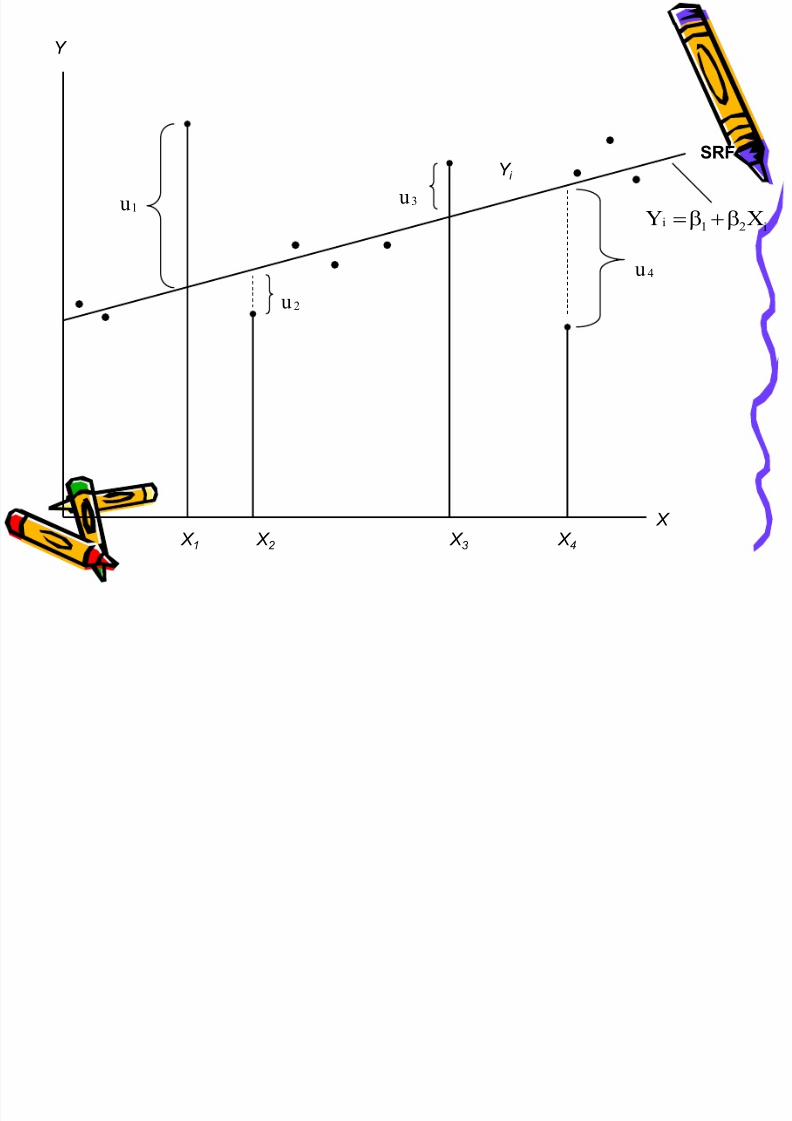
• See Figure: If all the observations were to lie on
the regression line, we would obtain a “perfect”
fit.
Y
8/21/2019 Application of Econometrics in Economics
http://slidepdf.com/reader/full/application-of-econometrics-in-economics 100/160
X
X 1 X 2 X 3 X 4
SRFY i
1u
2u
3u
4u
i 1 2 iY X
• The concept of coefficient of determination can
8/21/2019 Application of Econometrics in Economics
http://slidepdf.com/reader/full/application-of-econometrics-in-economics 101/160
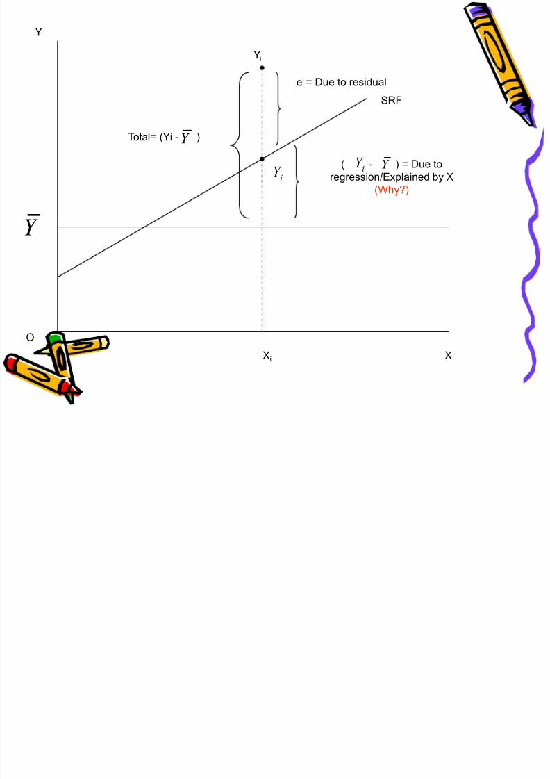
be explained using the following diagram
Y
Y
8/21/2019 Application of Econometrics in Economics
http://slidepdf.com/reader/full/application-of-econometrics-in-economics 102/160
O
Xi X
Yi
Y
Total= (Yi - )Y
SRF
ei = Due to residual
( - ) = Due to
regression/Explained by X
(Why?)
iY ˆ Y
iY ˆ
• iiii Y Y Y Y Y Y ˆˆ

8/21/2019 Application of Econometrics in Economics
http://slidepdf.com/reader/full/application-of-econometrics-in-economics 103/160
- Mean of the sample data
- Predicted value of Y for a given X (Point on
SRF)
- An individual sample observation
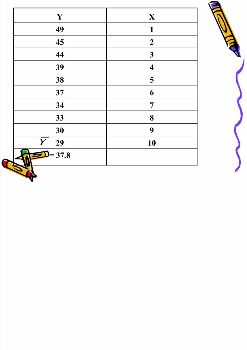
• Numerical proof (Consider following
example)
iiii
iY
Y
iY
Y X
8/21/2019 Application of Econometrics in Economics
http://slidepdf.com/reader/full/application-of-econometrics-in-economics 104/160
49 1
45 2
44 3
39 4
38 5
37 6
34 7
33 8
30
9
29 10
= 37.8
Y
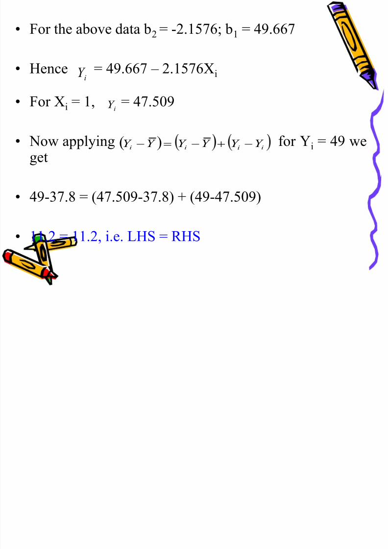
• For the above data b2 = -2.1576; b1 = 49.667
8/21/2019 Application of Econometrics in Economics
http://slidepdf.com/reader/full/application-of-econometrics-in-economics 105/160
2 1
• Hence = 49.667 – 2.1576Xi
• For Xi = 1, = 47.509
• Now applying for Yi = 49 weget
• 49-37.8 = (47.509-37.8) + (49-47.509)
• 11.2 = 11.2, i.e. LHS = RHS
iY ˆ
iY ˆ
iiii Y Y Y Y Y Y ˆˆ
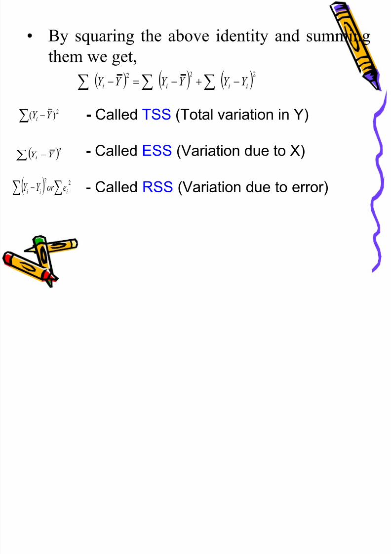
• By squaring the above identity and summing
8/21/2019 Application of Econometrics in Economics
http://slidepdf.com/reader/full/application-of-econometrics-in-economics 106/160
By squaring the above identity and summing
them we get,
- Called TSS (Total variation in Y)
- Called ESS (Variation due to X)
- Called RSS (Variation due to error)
222 ˆˆ
iiii Y Y Y Y Y Y
2)( Y Y i
2ˆ Y Y i
2
2ˆ
iii eor Y Y
• Thus, TSS = ESS + RSS
8/21/2019 Application of Econometrics in Economics
http://slidepdf.com/reader/full/application-of-econometrics-in-economics 107/160
• If all actual Ys lie on fitted SRF, RSS=0 and hence
ESS=TSS (Polar cases)
• If X explains no variation in Y, ESS=0 and hence
RSS=TSS (Polar cases)
• If ESS is relatively larger than RSS, then the chosen
SRF fits the data well
• If RSS is relatively larger than ESS, then the chosen
SRF fits the data poorly
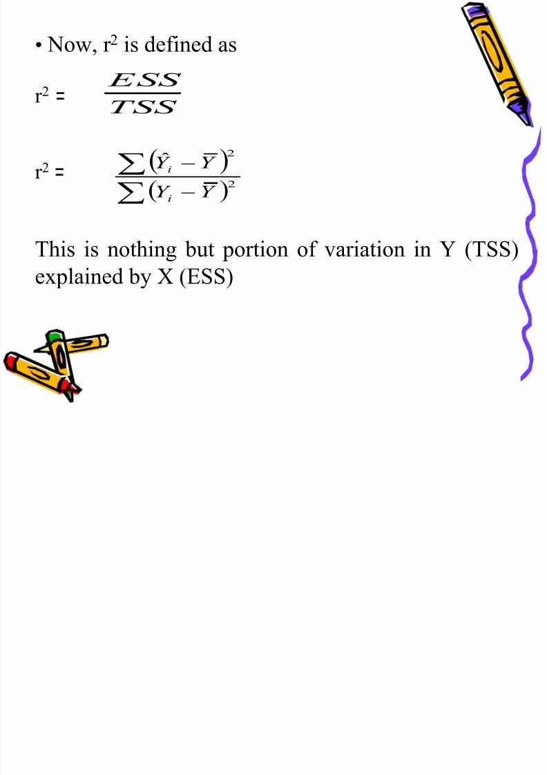
• Now, r 2 is defined as
8/21/2019 Application of Econometrics in Economics
http://slidepdf.com/reader/full/application-of-econometrics-in-economics 108/160
,
r 2 =
r 2 =
This is nothing but portion of variation in Y (TSS)
explained by X (ESS)
TSS
ESS
2
2ˆ
Y Y
Y Y
i
i
Properties of r2
8/21/2019 Application of Econometrics in Economics
http://slidepdf.com/reader/full/application-of-econometrics-in-economics 109/160
• It is a nonnegative quantity (Why?)
• Its limits are 0 r 21
• An r 2
of 1 means a perfect fit, that is, foreach i.
• An r 2 of zero means that there is no relationship
between Y and X
ii Y Y ˆ
• Example: In a regression with quantity
8/21/2019 Application of Econometrics in Economics
http://slidepdf.com/reader/full/application-of-econometrics-in-economics 110/160
demanded as dependent variable and price
independent variable an r 2
value of 0.975implies that price variable explains about 98%
of variation in quantity demanded . In this case,
we can say that sample regression gives an
excellent fit.
Coefficient of correlation (r)
8/21/2019 Application of Econometrics in Economics
http://slidepdf.com/reader/full/application-of-econometrics-in-economics 111/160
• It measures degree of linear association
between Y and X
• It is nothing but
• In practice r is of little importance
• The more meaningful quantity is r 2 (Why?)
• r is also called simple correlation coefficient orcorrelation coefficient of zero order
2r
• Interpretation of r: r 12 means correlation
8/21/2019 Application of Econometrics in Economics
http://slidepdf.com/reader/full/application-of-econometrics-in-economics 112/160
p 12
between variable 1 (say Y) and variable 2 (say
X2)
Standard Error (SE) of Regression Coefficients
8/21/2019 Application of Econometrics in Economics
http://slidepdf.com/reader/full/application-of-econometrics-in-economics 113/160
• We know that least-squares estimates (b1 and b2)
are estimated using sample data
• But since data are likely to change from sample
to sample, the estimates will change as well
• Therefore, what is needed is some measure of
“reliability” of OLS estimators
• The precision of an estimate or regression
coefficient is measured by SE
• SE is the standard deviation (positive square rootof variance) of sampling distribution (SD) of the
8/21/2019 Application of Econometrics in Economics
http://slidepdf.com/reader/full/application-of-econometrics-in-economics 114/160
of variance) of sampling distribution (SD) of theestimator (say b2)
• SD of an estimator is a distribution of set ofvalues of estimator obtained from all possible
samples of same size from a given population.
• Thus, SE of an estimator is the amount it varies
across samples.
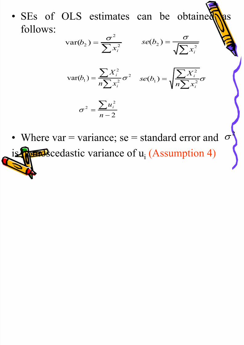
• SEs of OLS estimates can be obtained as
f ll
8/21/2019 Application of Econometrics in Economics
http://slidepdf.com/reader/full/application-of-econometrics-in-economics 115/160
follows:
• Where var = variance; se = standard error and
is homoscedastic variance of ui (Assumption 4)
2
2
2 )var(i x
b
2
2 )(
i x
b se
2
2
2
1 )var(
i
i
xn
X b
2
2
1)(i
i
xn
X b se
2
2
ˆ
ˆ
2
2
n
ui
• Here the variance of b2 is inversely proportional to 2
i x
8/21/2019 Application of Econometrics in Economics
http://slidepdf.com/reader/full/application-of-econometrics-in-economics 116/160
• That is, given , larger the variation in X values, the
smaller the variance of b2 and hence greater the
precision with which b2 can be estimated.
• In short, if there is substantial variation in Xs (recallAssumption 8), b2 can be measured more accurately
than when Xs do not vary substantially.
2
• Hence, what is a „big‟ SE of regression
coefficients and what is a „small‟ SE depends on
8/21/2019 Application of Econometrics in Economics
http://slidepdf.com/reader/full/application-of-econometrics-in-economics 117/160
coefficients and what is a small SE depends on
the context (i.e. variation in Xs)
• A more standardized statistic, which also gives a
measure of the „goodness of fit‟ of estimated
equation is R 2
• SEs of regression coefficients can be used for
hypothesis testing and constructing confidenceintervals (discussed later)
Standard Error of Regression/Residuals
8/21/2019 Application of Econometrics in Economics
http://slidepdf.com/reader/full/application-of-econometrics-in-economics 118/160
• SE of regression is the standard deviation
(Positive square root of variance) of individual Yvalues about the estimated regression line or
error term
• If SE of residuals is high, then deviation will also
be high and hence fitness will be poor
• SE of residuals can be obtained using the
f ll i f l

8/21/2019 Application of Econometrics in Economics
http://slidepdf.com/reader/full/application-of-econometrics-in-economics 119/160
following formula
2
ˆ
ˆ
22
2
2
n
xb y ii

8/21/2019 Application of Econometrics in Economics
http://slidepdf.com/reader/full/application-of-econometrics-in-economics 120/160
Multiple Regression Analysis
Meaning
8/21/2019 Application of Econometrics in Economics
http://slidepdf.com/reader/full/application-of-econometrics-in-economics 121/160
• In single/two variable model there is only one
explanatory variable
• In practice, most problems can‟t be explained by
this model
• Example: Apart from prices, demand is a function
of many other factors
• Hence, we use multiple regression models whichcontain more than one Xs
How the model looks like?
8/21/2019 Application of Econometrics in Economics
http://slidepdf.com/reader/full/application-of-econometrics-in-economics 122/160
•
PRF for cross sectional data•
PRF for time-series data
• Any individual Y value can be expressed assum of 2 components
Deterministic component [E (Yi)]
Random component [ ]
iiii U X B X B BY 33221
t t t t U X B X B BY 33221
ii X B X B B 33221
iU
Assumptions
8/21/2019 Application of Econometrics in Economics
http://slidepdf.com/reader/full/application-of-econometrics-in-economics 123/160
p
All the assumptions of two-variable
model are applicable in the case of
multiple regression as well
Eq.
8/21/2019 Application of Econometrics in Economics
http://slidepdf.com/reader/full/application-of-econometrics-in-economics 124/160
• It gives conditional mean value of Y
conditional upon the given/fixed values of Xs
• Symbolically
• Thus, what we obtain is the mean value of Y for
the given values of Xs
iiiii X B X B B X X Y E
3322132 ,
(PRCs)
8/21/2019 Application of Econometrics in Economics
http://slidepdf.com/reader/full/application-of-econometrics-in-economics 125/160
• In multiple regression B2&B3 are called PRCs
• B2 measures change in the mean value of Y per
unit change in X2, holding value of X3 constant
[OR]
B2 gives “direct” or “net” effect of a unit change
in X2 on E(Y), net of any effect that X3 may have
on mean Y
• Similar explanation is applicable for B2 as well
Estimating PRCs
8/21/2019 Application of Econometrics in Economics
http://slidepdf.com/reader/full/application-of-econometrics-in-economics 126/160
• To estimate parameters of model we use OLS
method
• Let SRF corresponding to PRF described above
as:
• Where b1, b2 & b3 are estimators of unknown
population coefficients B1, B2 & B3 respectively
• ei is sample counterpart of residual term U
iiii e X b X bbY 33221
• OLS principle chooses values of unknown
t i h th t th RSS i2
8/21/2019 Application of Econometrics in Economics
http://slidepdf.com/reader/full/application-of-econometrics-in-economics 127/160
parameters in such a way that the RSS is as
small as possible
• Symbolically,
• Minimization of this involves differentiation
with respect to unknowns, setting resulting
expressions to zero, and solving themsimultaneously
2
ie
2
33221
2min iiii X b X bbY e
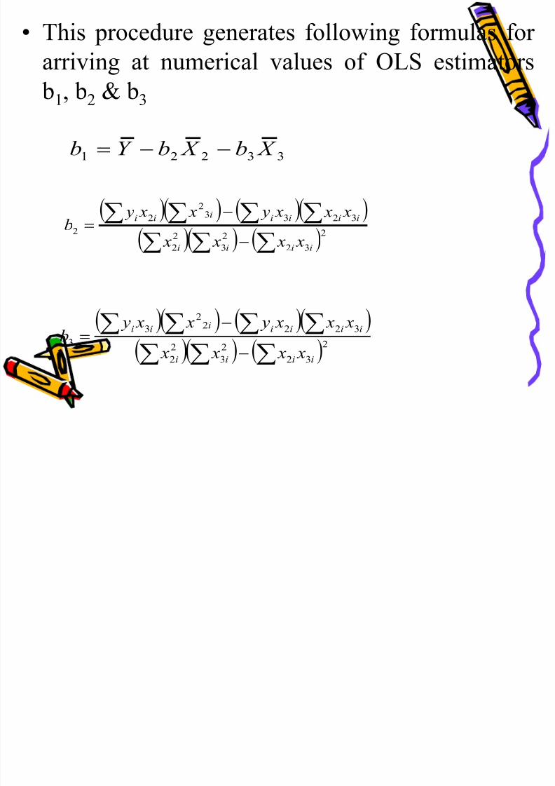
• This procedure generates following formulas for
arriving at numerical values of OLS estimators
8/21/2019 Application of Econometrics in Economics
http://slidepdf.com/reader/full/application-of-econometrics-in-economics 128/160
arriving at numerical values of OLS estimators
b1, b2 & b3
33221 X b X bY b
2
32
2
3
2
2
323322
2
iiii
iiiiiii
x x x x
x x x y x x yb
2
32
2
3
2
2
32222
3
3
iiii
iiiiiii
x x x x
x x x y x x yb
• In these formulas, lowercase letters denote
d i ti f l l
8/21/2019 Application of Econometrics in Economics
http://slidepdf.com/reader/full/application-of-econometrics-in-economics 129/160
deviations from sample mean values
Properties of OLS estimators

8/21/2019 Application of Econometrics in Economics
http://slidepdf.com/reader/full/application-of-econometrics-in-economics 130/160
The BLUE property continues to hold here aswell
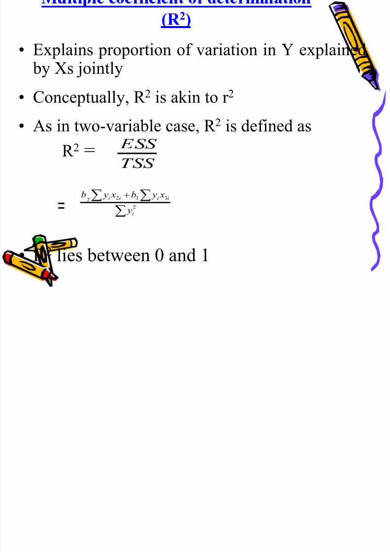
(R 2)
E l i ti f i ti i Y l i d
8/21/2019 Application of Econometrics in Economics
http://slidepdf.com/reader/full/application-of-econometrics-in-economics 131/160
• Explains proportion of variation in Y explained by Xs jointly
• Conceptually, R 2 is akin to r 2
• As in two-variable case, R 2 is defined as
R 2 =
=
• R 2 lies between 0 and 1
TSS ESS
2
3322
i
iiii
y
x yb x yb
• If R 2=1, fitted regression line explains
100% of variation in Y
8/21/2019 Application of Econometrics in Economics
http://slidepdf.com/reader/full/application-of-econometrics-in-economics 132/160
100% of variation in Y.
• If R 2=0, model does not explain any of the
variation in Y
• The fit of regression model is said to be
“better”, closer is R 2 to 1
• By and large, as the number of Xs increasesR 2 value increases (Why? See below)
R 2 and Adjusted R 2
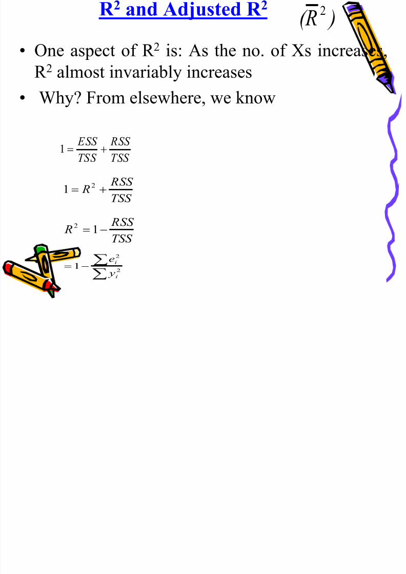
• One aspect of R2 is: As the no of Xs increases
) R( 2
8/21/2019 Application of Econometrics in Economics
http://slidepdf.com/reader/full/application-of-econometrics-in-economics 133/160
• One aspect of R 2 is: As the no. of Xs increases,
R 2 almost invariably increases
• Why? From elsewhere, we know
TSS
RSS
TSS
ESS
1
TSS
RSS R 21
TSS RSS R 12
2
2
1i
i
y
e
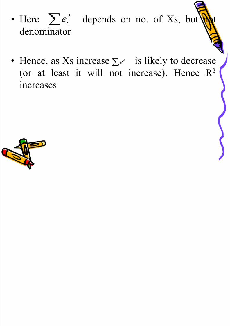
• Here depends on no. of Xs, but not
d i
2
ie
8/21/2019 Application of Econometrics in Economics
http://slidepdf.com/reader/full/application-of-econometrics-in-economics 134/160
denominator
• Hence, as Xs increase is likely to decrease
(or at least it will not increase). Hence R 2
increases
2
ie
Increasing R 2 • Is it desirable to increase R2 by adding more Xs?
8/21/2019 Application of Econometrics in Economics
http://slidepdf.com/reader/full/application-of-econometrics-in-economics 135/160
• Is it desirable to increase R by adding more Xs?
• We should adopt a cautious approach here
• Why?
(i) With larger Xs, R 2 gives an overly optimistic
picture of regression fit
(ii) R 2 does not take into account d.f.
(iii) We need to have a measure of goodness of fit thatis adjusted for no. of Xs added in the model
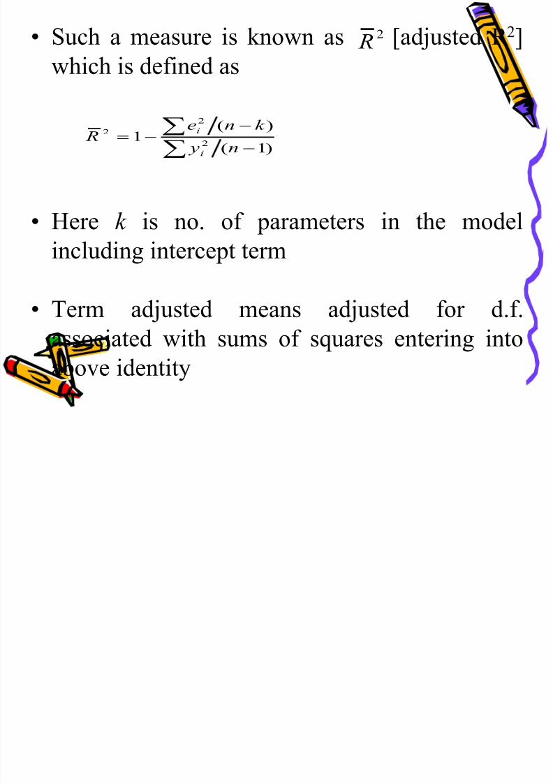
• Such a measure is known as [adjusted R 2]
which is defined as
2 R
8/21/2019 Application of Econometrics in Economics
http://slidepdf.com/reader/full/application-of-econometrics-in-economics 136/160
which is defined as
• Here k is no. of parameters in the model
including intercept term
• Term adjusted means adjusted for d.f.associated with sums of squares entering into
above identity
)1(
)(1
2
2
2
n y
k ne R
i
i
Features of Adjusted R 2
8/21/2019 Application of Econometrics in Economics
http://slidepdf.com/reader/full/application-of-econometrics-in-economics 137/160
• If k 1, R 2; i.e. as Xs increase becomes
increasingly less than R 2 or increases lessthan unadjusted R 2
• This means that, a penalty is involved in addingmore Xs in to a regression model
• can be negative, but not R 2 (Why?)
2 R
2 R
2 R
2 R
What we do in practice?
8/21/2019 Application of Econometrics in Economics
http://slidepdf.com/reader/full/application-of-econometrics-in-economics 138/160
• In practice, mainly R 2 is used to measure
“goodness” of fit
• is used in deciding inclusion of a newvariable
• If inclusion of a new variable increases , it isretained in the model
• When does increases? If value of thecoefficient of the added variable is larger than 1
2 R
2 R
2 R
t
Why maximizing opposed? 2 R
8/21/2019 Application of Econometrics in Economics
http://slidepdf.com/reader/full/application-of-econometrics-in-economics 139/160
• Our objective is not to obtain a high
• The researcher should be more concerned about
logical or theoretical relevance of the Xs to Yand their statistical significance
• If this process produces a high it is well andgood
2 R
2 R
Hypothesis Testing
8/21/2019 Application of Econometrics in Economics
http://slidepdf.com/reader/full/application-of-econometrics-in-economics 140/160
• The procedure is same as in two-variable case
• We can adopt both Confidence interval
approach and Test of significance approach
Testing under CIA
8/21/2019 Application of Econometrics in Economics
http://slidepdf.com/reader/full/application-of-econometrics-in-economics 141/160
• We construct a confidence interval and see
whether hypothesized value of population parameters (B1/ B2/ B3) lies inside this interval.
• If it lies inside, we do not reject H0
• If it lies outside, we can reject H0
• The remaining procedure is same as in the caseof two-variable model
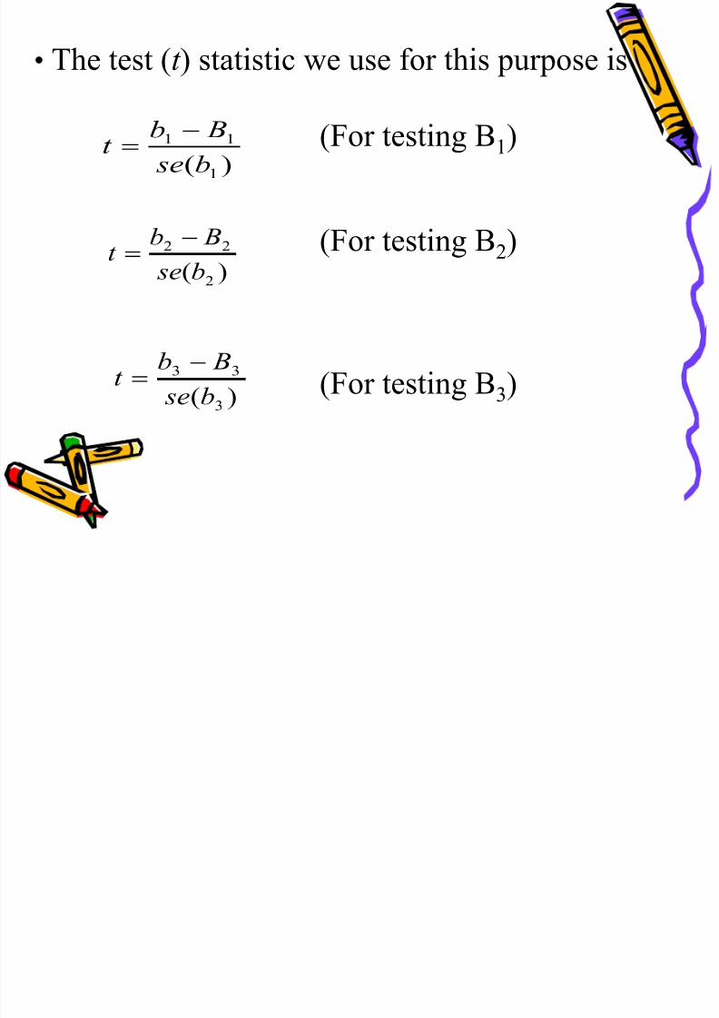
• The test (t ) statistic we use for this purpose is
8/21/2019 Application of Econometrics in Economics
http://slidepdf.com/reader/full/application-of-econometrics-in-economics 142/160
(For testing B1)
(For testing B2)
(For testing B3)
)( 1
11
b se
Bb
t
)( 2
22
b se
Bbt
)( 3
33
b se
Bbt
Testing under ToSA
8/21/2019 Application of Econometrics in Economics
http://slidepdf.com/reader/full/application-of-econometrics-in-economics 143/160
Step 1: Set H0 and H1 separately for each partial
regression coefficient
Examples: H0:B2 =0 and H1:B20H0:B3 =0 and H1:B30
Step 2: Compute a test (t ) statistic from sample
data (See above)
Step 3: Choose level of significance () (or) probability of committing Type 1 error
8/21/2019 Application of Econometrics in Economics
http://slidepdf.com/reader/full/application-of-econometrics-in-economics 144/160
(0.01 or 0.05 or 0.10)
Step 4: Find probability of obtaining computed test
(t ) statistic for certain d.f.
Note: d.f. is (n-k ), where n - no. of
observations, k- no. of Xs includingintercept term
Step 5: If this probability is less than the
prechosen reject H0. Otherwise, accept H0
8/21/2019 Application of Econometrics in Economics
http://slidepdf.com/reader/full/application-of-econometrics-in-economics 145/160
p j 0 p 0
(OR)
After Step 3 Use following rules to accept orreject H0
Null Hypothesis Alternative Critical region: Reject H0 if
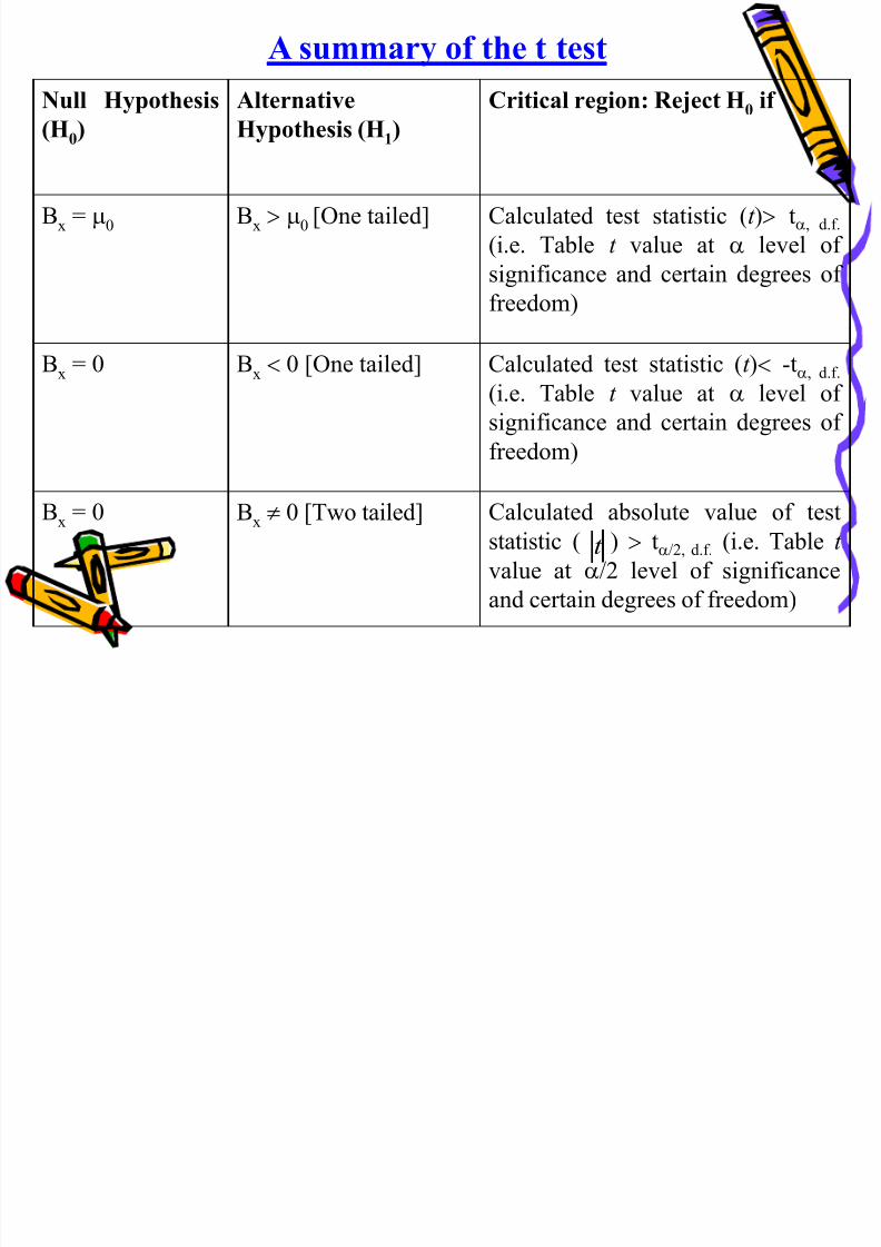
A summary of the t test
8/21/2019 Application of Econometrics in Economics
http://slidepdf.com/reader/full/application-of-econometrics-in-economics 146/160
(H0) Hypothesis (H1)
Bx = 0 Bx 0 [One tailed] Calculated test statistic (t ) t, d.f.
(i.e. Table t value at level of
significance and certain degrees of
freedom)
Bx = 0 Bx 0 [One tailed] Calculated test statistic (t ) -t, d.f.
(i.e. Table t value at level of
significance and certain degrees of
freedom)
Bx = 0 Bx 0 [Two tailed] Calculated absolute value of test
statistic ( ) t/2, d.f. (i.e. Table t
value at /2 level of significance
and certain degrees of freedom)
t
ANOVA or F test – Relevance
8/21/2019 Application of Econometrics in Economics
http://slidepdf.com/reader/full/application-of-econometrics-in-economics 147/160
• This is a complementary way of hypothesis
testing
• Commonly used to test joint H0 in multiple
regression models
• But, can be used in two variable regression model
as well
What is a joint H0?
8/21/2019 Application of Econometrics in Economics
http://slidepdf.com/reader/full/application-of-econometrics-in-economics 148/160
• H0: B2 = B3 = 0
• Means that B2 and B3 are jointly equal to zero
(or) Xs have no influence on Y
• A test of joint H0 is called a test of the overallsignificance of estimated regression line
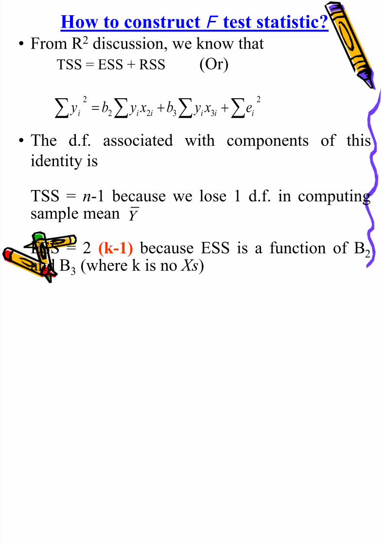
How to construct F test statistic?• From R 2 discussion, we know that
8/21/2019 Application of Econometrics in Economics
http://slidepdf.com/reader/full/application-of-econometrics-in-economics 149/160
TSS = ESS + RSS (Or)
• The d.f. associated with components of thisidentity is
TSS = n-1 because we lose 1 d.f. in computing
sample mean
ESS = 2 (k-1) because ESS is a function of B2 and B3 (where k is no Xs)
2
3322
2
iiiiii e x yb x yb y
Y
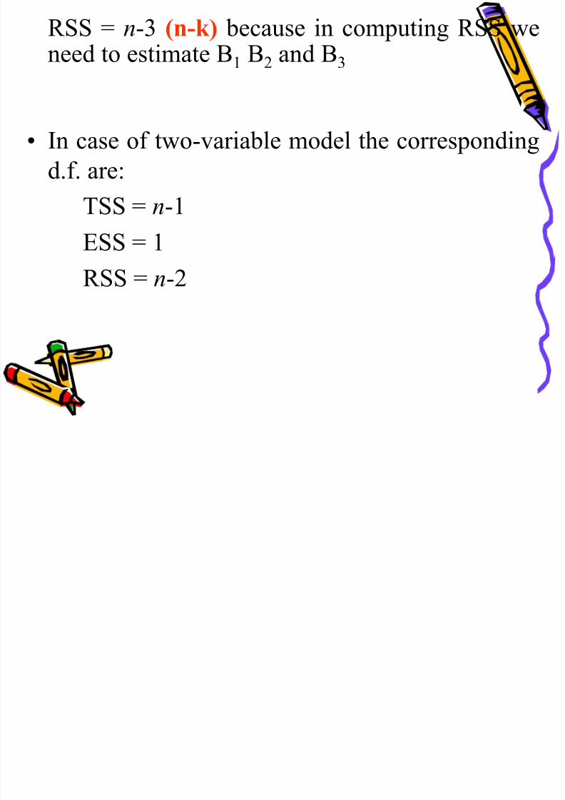
RSS = n-3 (n-k) because in computing RSS weneed to estimate B1 B2 and B3
8/21/2019 Application of Econometrics in Economics
http://slidepdf.com/reader/full/application-of-econometrics-in-economics 150/160
• In case of two-variable model the corresponding
d.f. are:
TSS = n-1ESS = 1
RSS = n-2
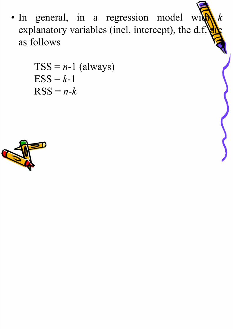
• In general, in a regression model with k
explanatory variables (incl. intercept), the d.f. are
8/21/2019 Application of Econometrics in Economics
http://slidepdf.com/reader/full/application-of-econometrics-in-economics 151/160
explanatory variables (incl. intercept), the d.f. are
as follows
TSS = n-1 (always)
ESS = k -1
RSS = n-k
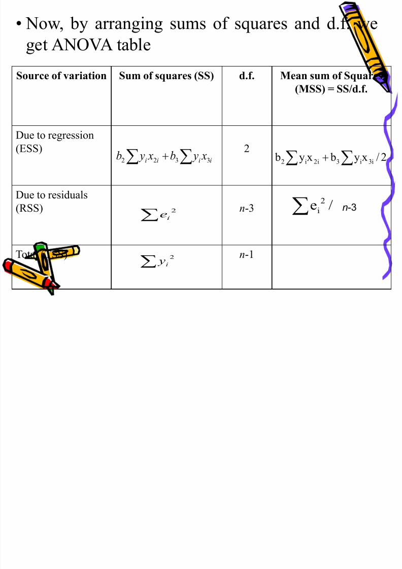
• Now, by arranging sums of squares and d.f. we
get ANOVA table
8/21/2019 Application of Econometrics in Economics
http://slidepdf.com/reader/full/application-of-econometrics-in-economics 152/160
Source of variation Sum of squares (SS) d.f. Mean sum of Squares
(MSS) = SS/d.f.
Due to regression
(ESS) 2
Due to residuals
(RSS) n-3 n-3
Total (TSS) n-1
iiii x yb x yb 3322
2
ie
2
i y
2 i 2i 3 i 3i b y x b y x / 2
2
ie /
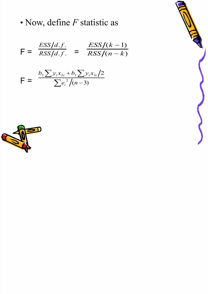
• Now, define F statistic as
8/21/2019 Application of Econometrics in Economics
http://slidepdf.com/reader/full/application-of-econometrics-in-economics 153/160
F = =
F =
..
..
f d RSS
f d ESS
)(
)1(
k n RSS
k ESS
)3(
2
2
3322
ne
x yb x yb
i
iiii
Using F-ratio for hypothesis testing
8/21/2019 Application of Econometrics in Economics
http://slidepdf.com/reader/full/application-of-econometrics-in-economics 154/160
• Set H0: B2 = B3 = 0 & H1: Not all Bs are
simultaneously zero
• Calculate F ratio using formula
• We reject H0, if F value computed from formulaexceeds critical/table F value at level ofsignificance and given d.f. in numerator anddenominator
• Otherwise, we do not reject H0:
• Alternatively, if the p value of computed F ratiois sufficiently low, we reject H0
8/21/2019 Application of Econometrics in Economics
http://slidepdf.com/reader/full/application-of-econometrics-in-economics 155/160
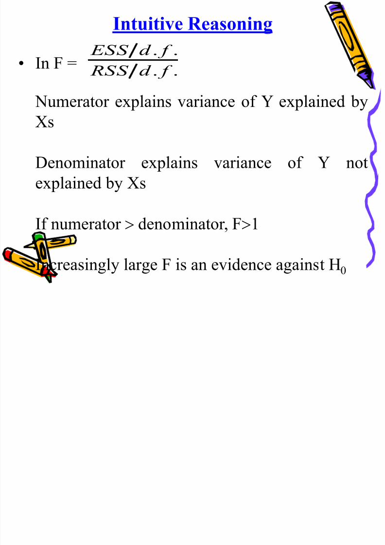
Intuitive Reasoning
.. f d ESS
8/21/2019 Application of Econometrics in Economics
http://slidepdf.com/reader/full/application-of-econometrics-in-economics 156/160
• In F =
Numerator explains variance of Y explained by
Xs
Denominator explains variance of Y not
explained by Xs
If numerator denominator, F1
Increasingly large F is an evidence against H0
.. f d RSS
f
Relationship between F and R 2
8/21/2019 Application of Econometrics in Economics
http://slidepdf.com/reader/full/application-of-econometrics-in-economics 157/160
• The null B2
= B3
= 0 is same as saying that H0
:
R 2=0 (why?)
• Thus, F test is also a test of significance of R 2
(i.e. whether R 2 is different from zero)
• The relationship between F ratio and R 2 is as
follows
• )/()1(
)1(2
2
knR
k R F
8/21/2019 Application of Econometrics in Economics
http://slidepdf.com/reader/full/application-of-econometrics-in-economics 158/160
• Here, when R 2=0, F=0
• The larger R 2 is, the greater the F value will be
• One advantage of this formula is the ease of
computation of F value. All we need to know isR 2 value
)/()1( k n R
Testing significance of R 2 using F test
S b tit t R2 l i d t F)1(
2kR
8/21/2019 Application of Econometrics in Economics
http://slidepdf.com/reader/full/application-of-econometrics-in-economics 159/160
• Substitute R 2 value in and compute F
ratio
• We reject H0: R 2=0, if F value computed from formulaexceeds the critical/table F value at level ofsignificance and given d.f. in numerator anddenominator
• Otherwise, we do not reject the null
)/()1(
)1(2
k n R
k R F
Usefulness of this statistic
8/21/2019 Application of Econometrics in Economics
http://slidepdf.com/reader/full/application-of-econometrics-in-economics 160/160
• In cross-sectional data involving severalobservations, one generally obtains low R 2
• This is due to diversity of the cross-sectional
units
• Here, the statistical significance of R 2 value can
be verified using)/()1(
)1(2
2
kR
k R F