Application of Data Fusion to

Aerial Robotics

Paul Riseborough

March 24, 2015

Outline

• Introduction to APM project

• What is data fusion and why do we use it?

• Where is data fusion used in APM?

• Development of EKF estimator for APM

navigation

– Problems and Solutions

• Future developments

• Questions

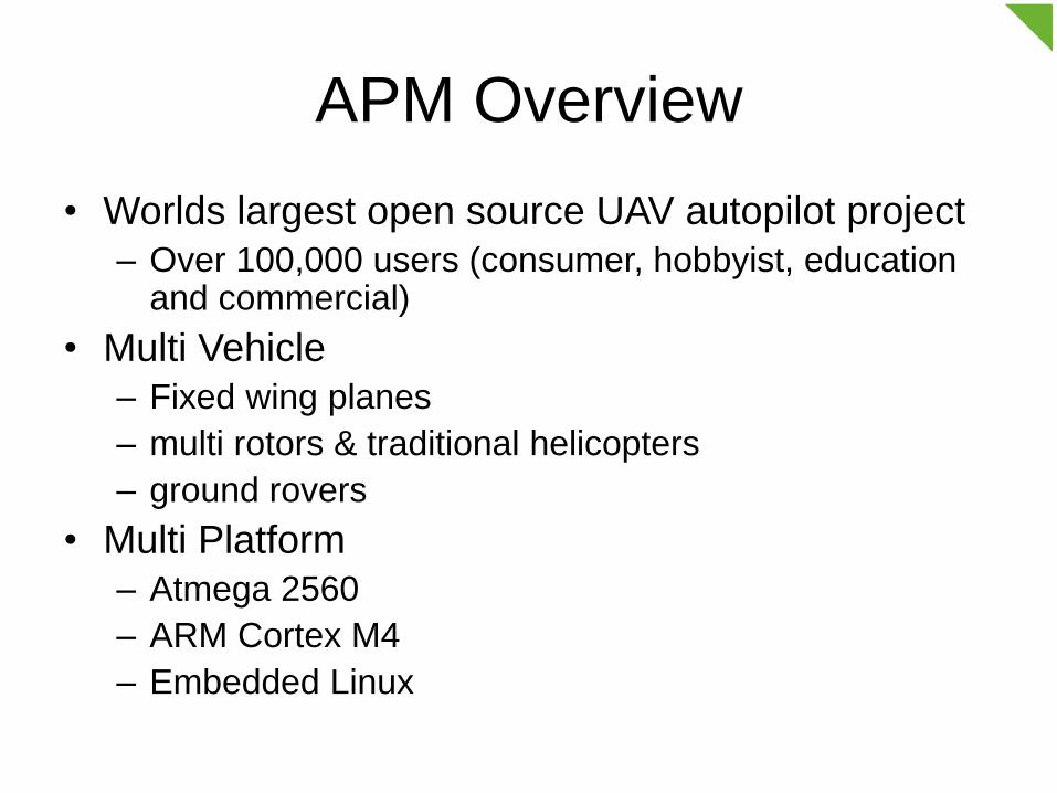
APM Overview

• Worlds largest open source UAV autopilot project

– Over 100,000 users (consumer, hobbyist, education and commercial)

• Multi Vehicle

– Fixed wing planes

– multi rotors & traditional helicopters

– ground rovers

• Multi Platform

– Atmega 2560

– ARM Cortex M4

– Embedded Linux

https://www.youtube.com/watch?v=XfvDwI4YVGk

Hardware Evolution

What is / Why Data Fusion

• In our context– Processing of data from multiple sources to estimate the internal

states of the vehicle

• Data fusion enables use of many low cost sensors to achieve required performance and robustness– Faulty sensors can be detected

– Effect of sensor noise and errors can be reduced

– Complementary sensing modalities can be combined (inertial, vision, air pressure, magnetic, etc) to achieve robust estimation

• The ‘Holy Grail’ is reliable and accurate estimation of vehicle states, all the time, everywhere and using low cost sensors– Still the weakest link in the reliability chain

– Failure can result in un-commanded flight path changes and loss of control

Data Fusion in APM

• Used to estimate the following:

– Vehicle position, velocity & orientation

– Wind speed & direction

– Rate gyro and accelerometer offsets

– Airspeed rate of change

– Airspeed scale factor error

– Height above ground

– Magnetometer offset errors

– Compass motor interference

– Battery condition

Data Fusion in APM

• Techniques:

– Complementary Filters• Computationally cheap – can run on 8bit micros

• Used for inertial navigation on APM 2.x hardware

• Used to combine air data and inertial data for plane speed and height control

– Nonlinear Least Squares• Batch processing for sensor calibration

– Extended Kalman Filters• Airspeed sensor calibration, 3-states

• Flight vehicle navigation, 22-states, only on 32-bit micros

• Camera mount stabilisation, 9 states, only on 32-bit micros

Development of an EKF

Estimator for APM

What is an EKF?• Stand for ‘Extended Kalman Filter’

• Enables internal states to be estimated from measurements for non-linear systems

• Assumes zero mean Gaussian errors in model and measured data

Predict

States

Predict

Covariance

Matrix

Update

States

Update

Covariance

Matrix

Measurements

Measurement Fusion

IMU data

Prediction

variancescovariances

Multiply

‘innovations’ by

the ‘Kalman

Gain’ to get state

corrections

EKF Processing Steps

• The EKF always consists of the following stages:

– Initialisation of States and Covariance Matrix

– State Prediction

– Covariance Prediction

– Measurement Fusion which consists of• Calculation of innovations

• Update of states using the innovations and ‘Kalman Gains’

• Update of the ‘Covariance Matrix’

State Prediction

• A standard strap-down inertial navigation processing is

used to calculate the change in orientation, velocity and

position since the last update using the IMU data

• IMU data is corrected for earth rotation, bias and coning

errors

• Bias errors, scale factor errors and vibration effects are

the major error sources

• Inertial solution is only useful for about 5 to 10 seconds

without correction

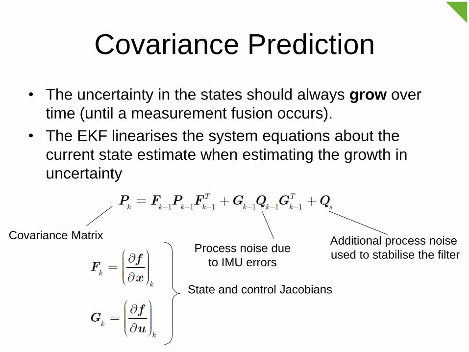
Covariance Prediction

• The uncertainty in the states should always grow over

time (until a measurement fusion occurs).

• The EKF linearises the system equations about the

current state estimate when estimating the growth in

uncertainty

Process noise due

to IMU errors

Additional process noise

used to stabilise the filter

State and control Jacobians

Covariance Matrix

state 1

state 2

When errors in states are

uncorrelated, the covariances

(off-diagonal elements) are

non-zero.When errors in states are

correlated the covariances

(off diagonal elements) are

non-zero.

What is the ‘Covariance Matrix’ ?

Defines the distribution of error for

each state and the correlation in

error between states Expected value

Measurement Fusion

• Updates the state estimates and covariance matrix using measurements.

• The covariance will always decrease after measurements are fused provided new information is gained.

Kalman Gain:

Innovation:

Covariance Update:

State Update:

Measurement covariance

Actual measurement

Predicted measurement

What is the ‘Innovation’ ?

• Difference between a measurement predicted by the filter and what is measured by the sensor.

• Innovations are multiplied by the ‘KalmanGain’ matrix to calculate corrections that are applied to the state vector

• Ideally innovations should be zero mean with a Gaussian noise distribution (noise is rarely Gaussian).

• Presence of bias indicates missing states in model

Innovation Example – GPS

Velocities

Taken from a flight of Skyhunter 2m wingspan UAV running

APMPlane on a Pixhawk flight computer and a u-blox LEA-6H

GPS

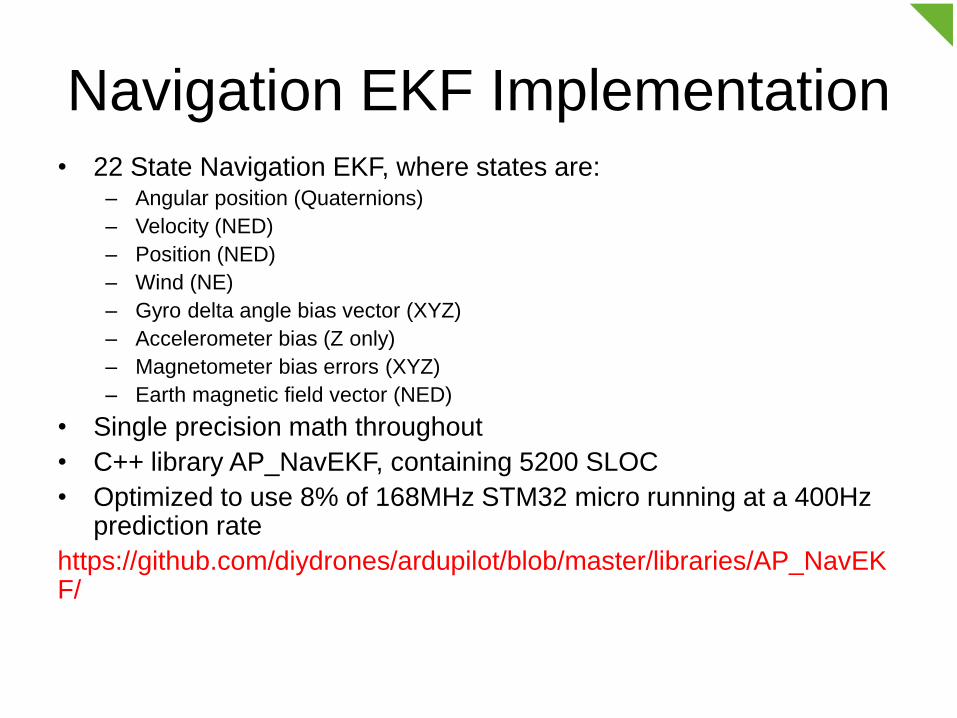
Navigation EKF Implementation• 22 State Navigation EKF, where states are:

– Angular position (Quaternions)

– Velocity (NED)

– Position (NED)

– Wind (NE)

– Gyro delta angle bias vector (XYZ)

– Accelerometer bias (Z only)

– Magnetometer bias errors (XYZ)

– Earth magnetic field vector (NED)

• Single precision math throughout

• C++ library AP_NavEKF, containing 5200 SLOC

• Optimized to use 8% of 168MHz STM32 micro running at a 400Hz prediction rate

https://github.com/diydrones/ardupilot/blob/master/libraries/AP_NavEKF/

Sensing• Dual IMU sensors (body angular rates and specific

forces)

– IMU data is used for state prediction only, it is not fused as

an observation

• GPS (Lat/Lon/Alt and local earth frame velocity)

• 3-Axis magnetometer

• Barometric Altitude

• True Airspeed

• Range finder (range to ground)

• Optical flow sensor (optical and inertial sensor

delta angles)

Problem 1: Processor Utilisation

• Significant emphasis on computational efficency...

– Limited processing: 168MHz STM32

– Ardupilot is single threaded

– 400Hz predictions, can’t take more than 1300micro sec (50% of total frame time)

• Implementation:

– Matlab Symbolic Toolbox used to derive algebraic equations.

– Symbolic objects are optimized and converted to C-code fragments using custom

script files. Current process is clunky. Mathworks proprietary converters cannot

handle problem size.

Efficient Algorithms

• Solutions: Covariance Prediction– Implemented as explicit algebraic equations (Matlab>>C)

• 5x reduction in floating point operations over matrix math for the covariance prediction

– Asyncronous runtime• Execution of covariance prediction step made conditional on time, angular movement and

arrival of observation data.

• Solutions: Measurement Fusion– Sequential Fusion: For computationally expensive sensor fusion steps (eg

magnetometer or optical flow), the X,Y,Z components can be fused sequentially, and if required, performed on consecutive 400Hz frames to level load

– Adaptive scheduling of expensive fusion operations, based on importance and staleness of data can be used to level load.

– Exploit sparseness in observation Jacobian to reduce cost of covariance update

• Problems– Stability: sequential fusion reduces filter stability margins >> care is taken to

maintain positive variances (diagonals) and symmetry of covariance matrix

– Jitter: Jitter associated with servicing sensor interrupts. Recent improvements to APM code have significantly reduced problems in this area

Problem 2: Bad Data

• Broad consumer/commercial adoption of Ardupilot = lots of corner

cases

• Over 90% of development work is about ‘corner cases’ relating to

bad sensor data including:

– IMU gyro and accelerometer offsets

– IMU aliasing due to platform vibration

– GPS glitches and loss of lock

– Barometer drift

– Barometer disturbances due to aerodynamic effects (position error, ground

effect, etc)

– Magnetometer calibration errors and electrical interference

– Range finder drop-outs and false readings

– Optical flow dropouts and false readings

Solutions for Bad Data

• IMU bias estimation (XYZ gyro and Z accel)

– XY accel bias is weakly observable for gentle flight profiles and is difficult to learn

in the time frame required to be useful

• Innovation consistency checks on all measurements

• Rejection Timeouts

– Dead reckoning only possible for up to 10s with our cheap sensors

– GPS and baro data rejection has a timeout followed by a reset to sensor data

• GPS glitch recovery logic

– Intelligent reset to match inertial sensors after large GPS glitch

• Aliasing Detection

– If GPS vertical velocity and barometer innovations are same sign and both

greater than 3-Sigma, aliasing is likely.

• Dual accelerometers combined with variable weighting

– Weighting based on innovation consistency (lower innovation = higher weight)

– Different sample rates reduce likelihood both will alias badly

Problem 3: Update Noise

• ‘Text Book’ implementation of an EKF produces steps in state estimates when observations are fused and states updated.

– APM multirotor cascaded control loops are vulnerable to this type of noise due to use of cascaded PID controllers and lack of noise filtering on motor demands.

• Solved by applying state correction incrementally across time to next measurement

– Reduces filter stability margins

‘truth’States Predicted

Using Inertial Data Corrections From Fusing

Measurements

time

state

Problem 4: Measurement Latency

• Observations (eg GPS) are delayed relative to inertial (IMU) data– Introduces errors and filter stability

• Potential Solutuions

1. Buffer state estimates and use stored state from measurement time horizon when calculating predicted measurement used for data fusion step.

– Assumes covariance does not change much across internal from measurement time horizon to current time

– Not good for observations in body frame that have significant delays

– Computationally cheap and is method used by current APM EKF

2. Buffer IMU data and run EKF behind real time with a moving fusion time horizon. Use buffered inertial data to predict the EKF solution forward to the current time horizon each time step

– Too memory and computationally expensive for implementation on STM32

3. Same as 2. but a simple observer structure is used to maintain a state estimate at the current time horizon that tracks the delayed filter estimate at the delayed time horizon

– Recent theoretical work by Alireza Khosravian from ANU (Australian National University)

– Robustness benefits of option 2, but computationally cheap enough to run on an STM32

– Will be implemented in future APM

Optical Flow Fusion• Why?

– Outdoor landing and takeoff

– Indoor station keeping

• Uses a PX4Flow smart camera

• Images and gyro rates sampled at 400Hz

• Shift between images converted to

equivalent angular rate

– Flow Rate = pixels_moved / delta_time *

pixels_per_radian

• Gyro and flow rates accumulated as delta

angles and used by the EKF at 10Hz

• Observability

– If velocity is non-zero and known (eg GPS),

height is observable– If height is known, velocity is observable

Velocity

Angular Rate

Range

Flow rate = Angular Rate + Velocity / Range

Optical Flow Design Challenges

• Accurate time alignment of gyro and flow measurements required

– Misalignment causes coupling between body angular motion and LOS rates which

destabilizes velocity control loop.

– Effect of misalignment worsens with height

• Focal length uncertainty and lens distortion

– Causes coupling between body angular motion and LOS rates which destabilizes

velocity control loop.

– Can vary 10% from manufacturers stated value

– Sensors must allow for storage of calibration coefficients

– Can be estimated in flight given time

• Assumption of flat level terrain

• Scale errors due to poor focus, contrast

– Innovation consistency checks

• Moving background

Optical Flow On Arducopter

• https://www.youtube.com/watch?v=9kBg0j

EmhzM

Where To Next?

• Lessons Learned:

– Large efficiency gains using scalar operations on the STM32 micro compared to

‘brute-force’ matrix math

– Stability challenges due to single precision maths

– It’s all about the corner cases!

– 90% of code maintenance has been in the state machine and related data checks

Where To Next?

• New derivation for pose estimation based on use of a rotation vector

for attitude estimation "Rotation Vector in Attitude Estimation", Mark E. Pittelkau,

Journal of Guidance, Control, and Dynamics, 2003

– Prototype in Ardupilot: 9-state gimbal estimator

– Reduces computational load (3 vs 4 attitude states)

– Reduces issues with linearization of quaternion parameters with large state

uncertainty.

– Enables bootstrap alignment from unknown initial orientation on moving platforms

including gyro bias estimation

– https://github.com/diydrones/ardupilot/blob/master/libraries/AP_NavEKF/AP_SmallE

KF.cpp

Where To Next?

• Tightly Coupled GPS fusion:

– Use individual satellite pseudo range and range rate observations.

– Better robustness to multi-path

– Eliminate reliance on receiver motion filter

– Requires double precision operations for observation models

• Move to a more flexible architecture that enables vehicle specific state

models and arbitrary sensor combinations

– Enables full advantage to be taken of multiple IMU units

– Use of vehicle dynamic models extends period we can dead-reckon without GPS.

– Requires good math library support (breaking news - we now have Eigen 3 support

in PX4 Firmware!!)

Flexible Architecture State Estimator • Common and platform/application

specific states in separate regions in

the state vector and covariance

matrix

• Use of Eigen matrix library to take

advantage of sparseness and

structure

• Generic observation models

• Position

• Velocity

• Body relative LOS rate

• Inertial LOS rate

• Body relative LOS angle

• Inertial LOS angle

• Range

• Delta Range

• Delta Range Rate

• Airspeed

• Magnetometer

Common States

Covariance Matrix

Platform Specific States

Questions?paul@3drobotics.com

SUPPORTING SLIDES

DERIVATION OF FILTER

EQUATIONS

AP_NavEKF Plant Equations% Define the state vector & number of states

stateVector = [q0;q1;q2;q3;vn;ve;vd;pn;pe;pd;dax_b;day_b;daz_b;dvz_b;vwn;vwe;magN;magE;magD;magX;magY;magZ];

nStates=numel(stateVector);

% define the measured Delta angle and delta velocity vectors

da = [dax; day; daz];

dv = [dvx; dvy; dvz];

% define the delta angle and delta velocity bias errors

da_b = [dax_b; day_b; daz_b];

dv_b = [0; 0; dvz_b];

% derive the body to nav direction cosine matrix

Tbn = Quat2Tbn([q0,q1,q2,q3]);

% define the bias corrected delta angles and velocities

dAngCor = da - da_b;

dVelCor = dv - dv_b;

% define the quaternion rotation vector

quat = [q0;q1;q2;q3];

AP_NavEKF Plant Equations% define the attitude update equations

delQuat = [1;

0.5*dAngCor(1);

0.5*dAngCor(2);

0.5*dAngCor(3);

];

qNew = QuatMult(quat,delQuat);

% define the velocity update equations

vNew = [vn;ve;vd] + [gn;ge;gd]*dt + Tbn*dVelCor;

% define the position update equations

pNew = [pn;pe;pd] + [vn;ve;vd]*dt;

% define the IMU bias error update equations

dabNew = [dax_b; day_b; daz_b];

dvbNew = dvz_b;

% define the wind velocity update equations

vwnNew = vwn;

vweNew = vwe;

AP_NavEKF Plant Equations% define the earth magnetic field update equations

magNnew = magN;

magEnew = magE;

magDnew = magD;

% define the body magnetic field update equations

magXnew = magX;

magYnew = magY;

magZnew = magZ;

% Define the process equations output vector

processEqns =

[qNew;vNew;pNew;dabNew;dvbNew;vwnNew;vweNew;magNnew;magEnew;magDnew;magXnew;magYnew;magZnew];

AP_SmallEKF Plant Equations% define the measured Delta angle and delta velocity vectors

dAngMeas = [dax; day; daz];

dVelMeas = [dvx; dvy; dvz];

% define the delta angle bias errors

dAngBias = [dax_b; day_b; daz_b];

% define the quaternion rotation vector for the state estimate

estQuat = [q0;q1;q2;q3];

% define the attitude error rotation vector, where error = truth - estimate

errRotVec = [rotErr1;rotErr2;rotErr3];

% define the attitude error quaternion using a first order linearisation

errQuat = [1;0.5*errRotVec];

% Define the truth quaternion as the estimate + error

truthQuat = QuatMult(estQuat, errQuat);

% derive the truth body to nav direction cosine matrix

Tbn = Quat2Tbn(truthQuat);

% define the truth delta angle

% ignore coning acompensation as these effects are negligible in terms of

% covariance growth for our application and grade of sensor

dAngTruth = dAngMeas - dAngBias - [daxNoise;dayNoise;dazNoise];

% Define the truth delta velocity

dVelTruth = dVelMeas - [dvxNoise;dvyNoise;dvzNoise];

% define the attitude update equations

% use a first order expansion of rotation to calculate the quaternion increment

% acceptable for propagation of covariances

deltaQuat = [1;

0.5*dAngTruth(1);

0.5*dAngTruth(2);

0.5*dAngTruth(3);

];

truthQuatNew = QuatMult(truthQuat,deltaQuat);

% calculate the updated attitude error quaternion with respect to the previous estimate

errQuatNew = QuatDivide(truthQuatNew,estQuat);

% change to a rotaton vector - this is the error rotation vector updated state

errRotNew = 2 * [errQuatNew(2);errQuatNew(3);errQuatNew(4)];

AP_SmallEKF Plant Equations

% define the velocity update equations

% ignore coriolis terms for linearisation purposes

vNew = [vn;ve;vd] + [0;0;gravity]*dt + Tbn*dVelTruth;

% define the IMU bias error update equations

dabNew = [dax_b; day_b; daz_b];

% Define the state vector & number of states

stateVector = [errRotVec;vn;ve;vd;dAngBias];

nStates=numel(stateVector);

AP_SmallEKF Plant Equations