APPENDIX 10: ANALYSIS OF VARIANCE (ANOVA) Modern Marketing ...webuser.bus.umich.edu/feinf/modernmarketingresearch/Chapter_10... · Appendix 10: ANOVA Feinberg, Kinnear & Taylor: Modern

Appendix 10: ANOVA Feinberg, Kinnear & Taylor: Modern Marketing Research Page 1

APPENDIX 10: ANALYSIS OF VARIANCE (ANOVA)

supplemental material to the text of

Modern Marketing Research: Concepts, Methods, and Cases

by Feinberg, Kinnear, and Taylor

Statistical Analysis of Experiments

Analysis of variance (ANOVA) is among the main methods used in social science. Although it

is, strictly speaking, a special case of regression, the techniques associated with it have become

so rich that ANOVA is often treated as a special subject in itself. It is important to understand

exactly what its requirements and assumptions are, so let us start there: ANOVA can be applied

when the researcher is analyzing one intervally scaled dependent variable and one or more

nominally scaled independent variables.

ANOVA is often discussed in terms of three somewhat different procedures. (Before trying

to make sense of them, you may wish to go back and review the material on basic statistical

inference and regression in Chapters 8 and 9.) These three ANOVA procedures are:

Model I: Fixed Effects. In this model, the researcher makes inferences only about

differences among the j treatments actually administered, and about no other treatment that

might have been included. In other words, no interpolation between treatments is made. For

example, if the treatments were high, medium, and low advertising expenditures, no

inferences are drawn about advertising expenditures between these three levels.

Model II: Random Effects. In the second model, the researcher assumes that only a random

sample of the treatments about which he or she wants to make inferences has been used.

Here, the researcher would be prepared to interpolate results between treatments, if need be.

Model III: Mixed Effects. In the third model, the researcher has some fixed and some

random independent variables (treatments).

The major differences among these models relate to the formulas used to calculate sampling

error and to some data assumptions. We shall show the calculations only for the fixed-effects

model because the basic approach and the principles to be established are the same for the other

models. Also, in marketing research, most experiments fit the fixed-effects model, as the

experiments usually include all treatments that are relevant to the decision to be made.

Additional detail on calculations, especially for Models II and III, can be found in any standard

text on ANOVA models.

In applying the fixed-effects model, the researcher must make several assumptions about the

data. Specifically:

1. For each treatment population, j, the experimental errors are independent and normally

distributed about a mean of zero with an identical variance (this variance is determined as

part of the estimation procedure).

2. The sum of all treatment effects is zero.

3. In the calculations presented here, each treatment group has the same number of

observations. This assumption is not generally necessary, but it simplifies the calculations;

most ANOVA programs will not require this assumption.


In experimentation, the null hypothesis is that the treatment effects equal zero. If τj represents

the effect of treatment j, and the total number of treatments is t, we can write the null hypothesis

as

021 ==⋅⋅⋅==⋅⋅⋅== tj ττττ

or in the equivalent notation

),....,2,1(0 tjj ==τ

where j = a specific treatment. The alternative hypothesis is that

)....,2,1(0 tjj ==/τ

Note that this asserts that at least one of the treatments is nonzero, not that they all are. If the

treatments have had no effect, we would expect the scores on the dependent variable to be the

same in each group, so that the mean values would be the same in each group. So our null

hypothesis is equivalent to the statement that

µµµµ == j....21

where 1, 2, . . ., j represent treatment groups, and µ represents the mean for the entire population,

without regard to groups. So we see that ANOVA is essentially a procedure for simultaneously

testing for the equality of two or more means. In this way, it extends the usual (pooled) t-test for

the equality of the means of exactly two groups.

Completely Randomized Design

ANOVA applied to a completely randomized design (CRD) is called “one-way” ANOVA

because it is being applied to categories of exactly one independent variable. Table 10A.1

presents results generated by a CRD. The measures on the dependent variable, Y, are taken on

the test units. Here, there are four test units in each of three treatments, so we have 4 × 3 = 12

test units. The units are stores in the relevant geographic region where each of three coupon

plans was applied. The dependent variable is the number of cases of cola sold the day after the

different coupons were run in local newspapers. The treatments are the three categories of the

independent variable, T.

T1 Coupon plan 1

T2 Coupon plan 2

T3 Coupon plan 3

So, we have three treatments, 12 test units, and an interval-scaled measure on each test unit,

ensuring that ANOVA can be applied.


In Table 10A.1, we define the mean of each treatment group as

nMY

j

jj

∑==

.

..

Y

Table 10A.1 Completely Randomized Design with Three Treatments (Coupon Plans)

Treatments (j)

Coupon plan 1 Coupon plan 2 Coupon plan 3

Test units (i) 20 17 14

18 14 10

15 13 7

11 8 5

Treatment

totals 64Y.1 =∑ 52Y.2 =∑ 36Y.3 =∑

Treatment

means

1664/4

/nY

MY

1.1

.1.1

==

∑=

=

1352/4

/nY

MY

2.2

.2.2

==

∑=

=

936/4

/nY

MY

1.3

.3.3

==

∑=

=

Grand total 152365264..Y =++=∑

Grand mean

12.7152/12

)3

n2

n1

Y../(nM..Y

==

++== ∑

Note: n1 = n2 = n3 = nj = 4

The use of the period (.) in front of the j implies that we are calculating the mean by adding

all i’s in the jth treatment group. Note also that ∑Yi: indicates the sum of all j’s for given i, and

∑Y.. indicates the sum of all i’s and all j’s. In our example,

94

36

3.3.

134

52

2.2.

164

64

1.1.

==

==

==

MY

MY

MY

We also define the grand mean of all observations across all treatment groups as Y .. or M.

Here

7.1212

365264M =

++=

These various means will be used to interpret the results and calculations of an ANOVA. In

an experimental context, we want to determine whether the treatments have had an effect on the

dependent variable. (By “effect” we mean a functional relationship between the treatment Tj and


the dependent variable Y.) That is, do different treatments give systematically different scores on

the dependent variable? For example, in our coupon plan example, if the plans have had differing

effects on sales, we would expect the amount of sales in the stores in treatment T1 to differ

systematically from T2 and T3. If in fact they did, the mean of each treatment group would also

differ. In ANOVA, an effect is defined as a difference in treatment means from the grand mean.

What we are doing in ANOVA mirrors our development throughout all regression-based

statistical models: determining whether differences in treatment means are large enough to be

unlikely to have occurred just by chance alone.

Some Notation and Definitions

Let Yij be the score of the ith test unit on the jth treatment. For example, in Table 10A.1,

Y11 = 20; Y42 = 8, and so on.

We define any individual test unit’s scores as equal to

Yij = grand mean + treatment effect + error

or

Yij = µ + τj + Єij

This is a simple linear, additive model with values specified in terms of population parameters.

Because we are going to be using sample results to make inferences, we can translate this model

into the language of observable, sample quantities as

Yij = M + Tj + Eij

where M = the grand mean

Tj = the effect of the jth treatment

Eij = the statistical error of the ith test unit in the jth treatment

(Note that Eij plays the same role as eij in ordinary regression models. It is customary to

capitalize the “E” in ANOVA models, so we hew to that convention, but there is no conceptual

difference between Eij in ANOVA and eij in regression.)

In this model, the treatment effect is defined as the difference between the treatment mean

and the grand mean:

Tj = M..j – M

The reason we use M as the base from which to compare the various M.j’s is that even if we did

not know from which treatment a test unit came, we could still “guess” the grand mean as their

score on the dependent variable. Knowledge of treatment group memberships improves our

ability to predict scores, relative to simply using the overall mean, M.


The error for an individual unit, Eij, is estimated by the difference between an individual

score and the treatment group mean to which the score belongs.

Eij = Yij – M.j

It is a measure of the difference in scores that are not explained by treatments. This is the

measure of sampling error in the experiment, and is also referred to as experimental error. For

example, if all scores within a treatment are close together, the individual scores will be close to

the treatment mean, and the error will be small. So, this deviation is a measure of the random

variation within each treatment in an experiment.

We can rewrite this equation as

Yij = M + (M..j – M) + (Yij – M..j)

↓ ↓ ↓ ↓

Individual score = grand mean + treatment effect + error

Note that this rewritten form is an identity: we have just added and subtracted the same

quantities—the treatment mean (M.j) and the grand mean (M)—on the right side, so the equation

is in effect saying that Yij is equal to itself; it is just helpful as a way of decomposing various

effects. Alternatively, we can write any observation as a deviation from the grand mean. We do

this by moving M to the left side of this, creating yet another identity:

(Yij – M) = (M..j – M) + (Yij – M..j)

↓ ↓ ↓

Individual score deviation of individual score

deviation from = group mean + deviation from

grand mean from mean group mean

(i.e., treatment effect) (i.e., error)

Partitioning the Sum-of-Squares

The idea of ANOVA is built around the concept of partitioning, which means decomposing

some quantity into other quantities; these quantities will always be sums-of-squares. Specifically,

ANOVA relates the sum of squared deviations from the grand mean to that from group means, in

the following way. Begin by squaring the deviation from the grand mean, M, for each score in

the sample, and then sum these squared deviations across all test units, i, in all groups, j. Do this

by squaring the previous equation for all individuals in all groups; this becomes

( ) ( ) ( )[ ]∑=∑=

−+−=∑=∑=

−n

i

t

jjMijYMjM

n

i

t

jMijY

1 1

2..

1 1

2


All the ∑ =∑ =nj

ni 11

means is that we are doing this for all individuals in all treatments. This

equation can be expanded as follows (this is simply squaring an equation of the form “A = B +

C” to obtain “A2

= B2

+ C2

+ 2BC”):

( ) ( ) ( )( )∑

=∑

=−−+∑

=∑

=−+∑

=∑

=−=∑

=∑

=−

n

i

t

j

M.jij

YMj

Mn

i

t

j

Mij

Yn

i

t

j

Mj

Mn

i

t

j

Mij

Y

1 1.

2

1 1

2

1 1

2.

1 1

2)(

The sum of deviations (not squared deviations!) about any mean always equals zero*. Therefore,

it is not difficult to see (and demonstrate algebraically) that the ).)(.(11

2 jMijYMjMnj

ni

−−∑ =∑ =

portion of this equation must also be zero.

Also note that

∑ −=

=∑

=∑

=−

t

jjj MMn

n

i

t

j

Mj

M1

2

. )(1 1

2)

.(

where nj is the number of subjects in group j. This is so because M.j - M is a constant (as we are

dealing with means only) for each individual i in a particular group j. Our equation then becomes

( )∑=

∑=

−n

i

t

jMijY

1 1

2 = ( )∑

=−

t

jMMn jj

1

2. + ( )∑

=∑=

−n

i

t

jMijY j

1 1

2.

↓ ↓ ↓

weighted sum of

Total sum of squared deviations sum of squared

squared deviations = of group means + deviations within

from the grand mean from grand mean groups

Total sum of sum of squares sum of squares

squares (SST) = between groups + within groups

treatment effect error sum

sum of squares + of squares

(SSTR)

(SSE)

What we have done is divide (“partition”) the total sum-of-squares into two components.

These components are the sum-of-squares within groups and the sum-of-squares between groups.

These are each measures of variation. If the treatments have had no effect, the scores in all

treatment groups should be similar. If this were so, the variance of the sample calculated using

all test unit scores, without regard to treatment groups, would equal the variance calculated

within treatment groups. That is, the between-group variance would equal the within-group

variance. If the treatments have had an effect, however, the scores within groups would be more

similar than scores selected from the whole sample at random. That is, the variance taken within

* This basic statistical manipulation is easily illustrated: 10 + 5 + 15 = 30, and the mean is 30/3 = 10. The sum of

deviations is (10 – 10) + (5 – 10) + (15 – 10) = 0 + (–5) + 5 = 0.


groups would be smaller than the variance between groups, and we could compare the variance

between groups with the variance within groups as a way of measuring for the presence of an

effect. This is precisely what the statistical procedure does, and the reader should verify this

when reviewing the partitioning equations presented earlier.

But how do we get variance from the sum-of-squares terms we have in the current version of

our equation? Because variance equals SS/df, all we need to do is divide each component of the

equation by its appropriate df, and we will have the necessary variance terms. To obtain the

required degrees-of-freedom we apply the standard rule, as follows. For the sample as a whole,

we “used up” one degree of freedom to calculate the grand mean; therefore, the relevant number

of degrees of freedom for the SST is the total number of test units minus one. For the SSTR, the

number of degrees of freedom is always one less than the number of treatments, because once we

have determined t – 1 group means and the grand mean, the last group mean can take on only

one value. The degrees-of-freedom for the error term equals the number of test units minus the

number of treatment groups, because we only use the t within-group means to calculate the error

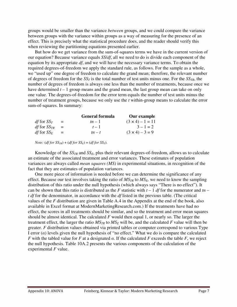
sum-of-squares. In summary:

General formula Our example

df for SST = tn – 1 (3 × 4) – 1 = 11

df for SSTR = t – 1 3 – 1 = 2

df for SSE = tn – t (3 × 4) – 3 = 9

Note: (df for SSTR) + (df for SSE) = (df for SST).

Knowledge of the SSTR and SSE, plus their relevant degrees-of-freedom, allows us to calculate

an estimate of the associated treatment and error variances. These estimates of population

variances are always called mean squares (MS) in experimental situations, in recognition of the

fact that they are estimates of population variances.

One more piece of information is needed before we can determine the significance of any

effect. Because our test involves taking the ratio of MSTR to MSE, we need to know the sampling

distribution of this ratio under the null hypothesis (which always says “There is no effect”). It

can be shown that this ratio is distributed as the F statistic with t – 1 df for the numerator and tn –

t df for the denominator, in accordance with the df listed in the previous table. (The critical

values of the F distribution are given in Table A.4 in the Appendix at the end of the book, also

available in Excel format at ModernMarketingResearch.com.) If the treatments have had no

effect, the scores in all treatments should be similar, and so the treatment and error mean squares

should be almost identical. The calculated F would then equal 1, or nearly so. The larger the

treatment effect, the larger the ratio MSTR to MSE will be, and the calculated F value will then be

greater. F distribution values obtained via printed tables or computer correspond to various Type

I error (α) levels given the null hypothesis of “no effect.” What we do is compare the calculated

F with the tabled value for F at a designated α. If the calculated F exceeds the table F, we reject

the null hypothesis. Table 10A.2 presents the various components of the calculation of the

experimental F value.


Table 10A.2 ANOVA Table for Completely Randomized Design

Source of variation Sum of squares

(SS)

Degrees of

freedom

(df)

Mean square

(MS)

F ratio

Treatments between

groups

SSTR t – 1

1t

SSMS

TRTR

−=

E

TR

MS

MS

Error (within groups) SSE tn – t

ttn

SSMS

EE

−=

Total SST tn – 1

A Calculated Example

We can now apply the developed methodology to see whether there is a significant treatment

effect for the data presented in Table 10A.1.

Total Sum-of-Squares*

( )( ) ( )

7.232

27.125

27.1217

2)7.1220(

1 1

2

=

−+⋅⋅⋅+−+−=

∑=∑=

−=n

i

t

jMijYTSS

Treatment Sum-of-Squares

( )

( ) ( )

7.98

27.129

27.12132)7.1216(4

1

2.

=

−+⋅⋅⋅+−+−=

∑=

−=

t

jMMnTRSS jj

Error Sum-of-Squares

( )

( ) ( )134

295

21317

2)1620(

1 1

2.

=

−+⋅⋅⋅+−+−=

∑=

∑=

−=n

i

t

jMijYESS j

Note that once we have obtained SST and SSTR, we can calculate SSE by subtracting SSTR from

SST. However, we can double-check our calculations by using the formula for SSE directly. By

applying the appropriate df to these SS values, we can obtain the mean squares necessary to

* We could, of course, use the computational formula for SS that was presented in Chapters 7 and 8.


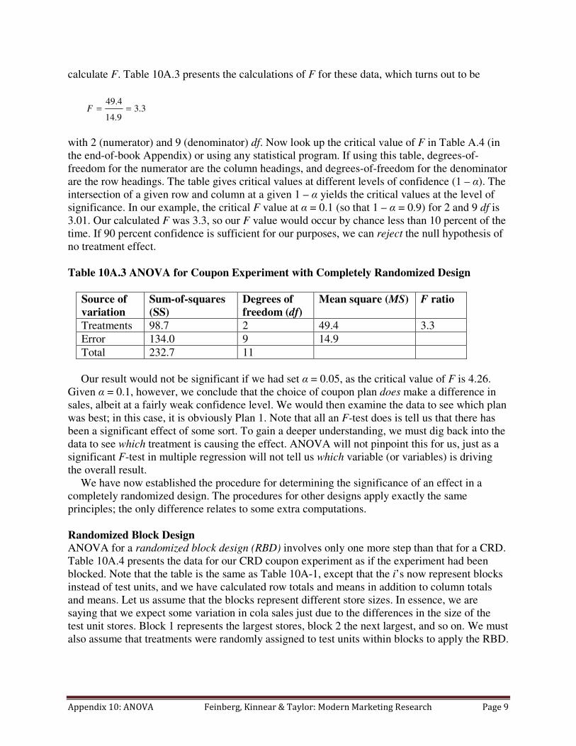
calculate F. Table 10A.3 presents the calculations of F for these data, which turns out to be

3.39.14

4.49==F

with 2 (numerator) and 9 (denominator) df. Now look up the critical value of F in Table A.4 (in

the end-of-book Appendix) or using any statistical program. If using this table, degrees-of-

freedom for the numerator are the column headings, and degrees-of-freedom for the denominator

are the row headings. The table gives critical values at different levels of confidence (1 – α). The

intersection of a given row and column at a given 1 – α yields the critical values at the level of

significance. In our example, the critical F value at α = 0.1 (so that 1 – α = 0.9) for 2 and 9 df is

3.01. Our calculated F was 3.3, so our F value would occur by chance less than 10 percent of the

time. If 90 percent confidence is sufficient for our purposes, we can reject the null hypothesis of

no treatment effect.

Table 10A.3 ANOVA for Coupon Experiment with Completely Randomized Design

Source of

variation

Sum-of-squares

(SS)

Degrees of

freedom (df)

Mean square (MS) F ratio

Treatments 98.7 2 49.4 3.3

Error 134.0 9 14.9

Total 232.7 11

Our result would not be significant if we had set α = 0.05, as the critical value of F is 4.26.

Given α = 0.1, however, we conclude that the choice of coupon plan does make a difference in

sales, albeit at a fairly weak confidence level. We would then examine the data to see which plan

was best; in this case, it is obviously Plan 1. Note that all an F-test does is tell us that there has

been a significant effect of some sort. To gain a deeper understanding, we must dig back into the

data to see which treatment is causing the effect. ANOVA will not pinpoint this for us, just as a

significant F-test in multiple regression will not tell us which variable (or variables) is driving

the overall result.

We have now established the procedure for determining the significance of an effect in a

completely randomized design. The procedures for other designs apply exactly the same

principles; the only difference relates to some extra computations.

Randomized Block Design

ANOVA for a randomized block design (RBD) involves only one more step than that for a CRD.

Table 10A.4 presents the data for our CRD coupon experiment as if the experiment had been

blocked. Note that the table is the same as Table 10A-1, except that the i’s now represent blocks

instead of test units, and we have calculated row totals and means in addition to column totals

and means. Let us assume that the blocks represent different store sizes. In essence, we are

saying that we expect some variation in cola sales just due to the differences in the size of the

test unit stores. Block 1 represents the largest stores, block 2 the next largest, and so on. We must

also assume that treatments were randomly assigned to test units within blocks to apply the RBD.


Table 10A.4 Randomized Block Design with Three Treatments and Four Blocks

Treatments (j)

Blocks (i)

Store

sizes

Coupon

plan 1

Coupon

plan 2

Coupon

plan 3

Bloc

k

totals

Block means

1 20 17 14 ∑Y1.=

51 173/51.1.1 === MY

2 18 14 10 ∑Y2.=

42

143/42.2.2 === MY

3 15 13 7 ∑Y3.=

35

7.113/35.3.3 === MY

4 11 8 5 ∑Y4.=

24 83/24.4.4 === MY

Treatment

totals ∑ =64Y.1 ∑ =52Y.2 ∑ =36Y.3

Treatment

means

16

64/4

/nY

MY

1.1

.1.1

=

=

∑=

=

13

52/4

/nY

MY

2.2

.2.2

=

=

∑=

=

9

36/4

/nY

MY

3.3

.3.3

=

=

∑=

=

Grand total 152365264Y.1 +++=∑

Grand mean ( )12.7152/12

3n

2n

1n/YMY ....

==

∑ ++==


In the RBD, we define an individual observation as

Yij = grand mean + treatment effect + block effect + error

or, in population parameter terms,

Yij = µ + τj + βi + Єij

As always, we will be estimating this model using sample data, so we state the model as

Yij = M + Tj + Bi + Eij

where Bi is the effect of the ith block, and the other terms are defined as in the CRD. We have

previously defined the M and Tj items in this model, but we must define the blocking effect and

also re-define the error term. We define blocking effect in a parallel manner to the treatment


.iM

effect, the only difference being that the blocking effect is stated in terms of row means instead

of column means.

Bi = (Mi. – M)

Here, knowledge of blocking group membership improves our ability to predict scores as an

improvement over the grand mean. We assume that ;01 =∑ = ini B that is, the net block effect is

zero. We can rewrite our equation for the individual score (Yij) as

Yij = M + (M.j – M) + (M.i – M) + Eij

↓ ↓ ↓ ↓ ↓

Individual score = grand mean + treatment effect + blocking effect + error

We can then solve this equation for Eij to obtain the measurement of error effect.

( ) ( )

( )....

..

..

or ijijijij

ijij

ijijij

MMMYMMMY

MMMMMY

MMMMMYE

−+++−−=

+−+−−=

−−−−−=

The error terms thus represent the difference between an individual score, Yij, and the net

difference between the grand mean and the sum of the treatment and block means. If the

blocking effect is significant, this error will be smaller than an error defined without blocking.

As an illustration, consider score Y21 in Table 10A.4. This score is 18, and the error without

blocking is

Yij – M.j = 18 – 16 =2

With blocking, the error is

Yij + M – M.j – Mi. = 18 + 12.7 –16 –14 = 0.7

A similar pattern would be evident were this analysis performed on the other scores. The main

point is this: blocking serves to reduce the size of experimental error, on average.

Note that we may rewrite the equation for Yij as

Yij = M + (M.j – M) + ( – M) + (Yij – M.j – Mi. + M)

If we move M to the left side of the equation, sum the resultant deviations across all blocks and

all treatments, and square both sides, we obtain

( ) ( ) ( ) ( )∑∑∑ ∑∑∑= == ===

−−++−+−=−n

i

t

j

ijij

n

i

n

i

i

t

j

j

t

j

ij MMMYMMtMMnMY1 1

2

..

1 1

2

.

1

2

.

1

2


You may recognize this result as

SST = SSTR + SSB + SSE

It follows from the fact that all the cross-products again become zero, because each involves a

sum of individual deviations about a mean. Also, we may write

( ) ( )∑∑∑= ==

−−n

i

t

j

i

n

i

i MMMMt1 1

2

.

1

2

. ofinstead

because we are again adding constant means over the t treatments. That is, multiplying by t is

exactly the same as adding the same thing t times, and is precisely what was used in CRD.

The relevant df for the block is n – 1, because once any (n – 1) block means are specified, the

remaining one is automatically determined, given the grand mean value. If we subtract the

treatment and block degrees-of-freedom from the total degrees-of-freedom, we obtain the error

degrees-of-freedom as

Error df = total df – treatment df – block df

= (tn – 1) – (t – 1) – (n – 1)

= tn + 1 – t – n

In our example, the error df = (3 × 4) + 1 – 3 – 4 = 6. More generally, the same result may be

obtained by applying the formula

Error df = (t – 1) (n – 1)

Table 10A.5 presents the ANOVA table for an RBD.

Table 10A.5 ANOVA Table for Randomized Block Design

Source of variation Sum of

squares (SS)

Degrees of

freedom (df)


Treatments (between

columns)

SSTR t – 1

1t

SSMS

TRTR

−=

E

TR

MS

MS

Blocks (between

rows)

SSB n – 1

1n

SSMS

BB

−=

E

B

MS

MS

Error SSE (t – 1) (n – 1)

( )( )1n1t

SSMS

EE

−−=

Total SST tn – 1


We shall now apply the RBD ANOVA procedure to the data in Table 10A.4.


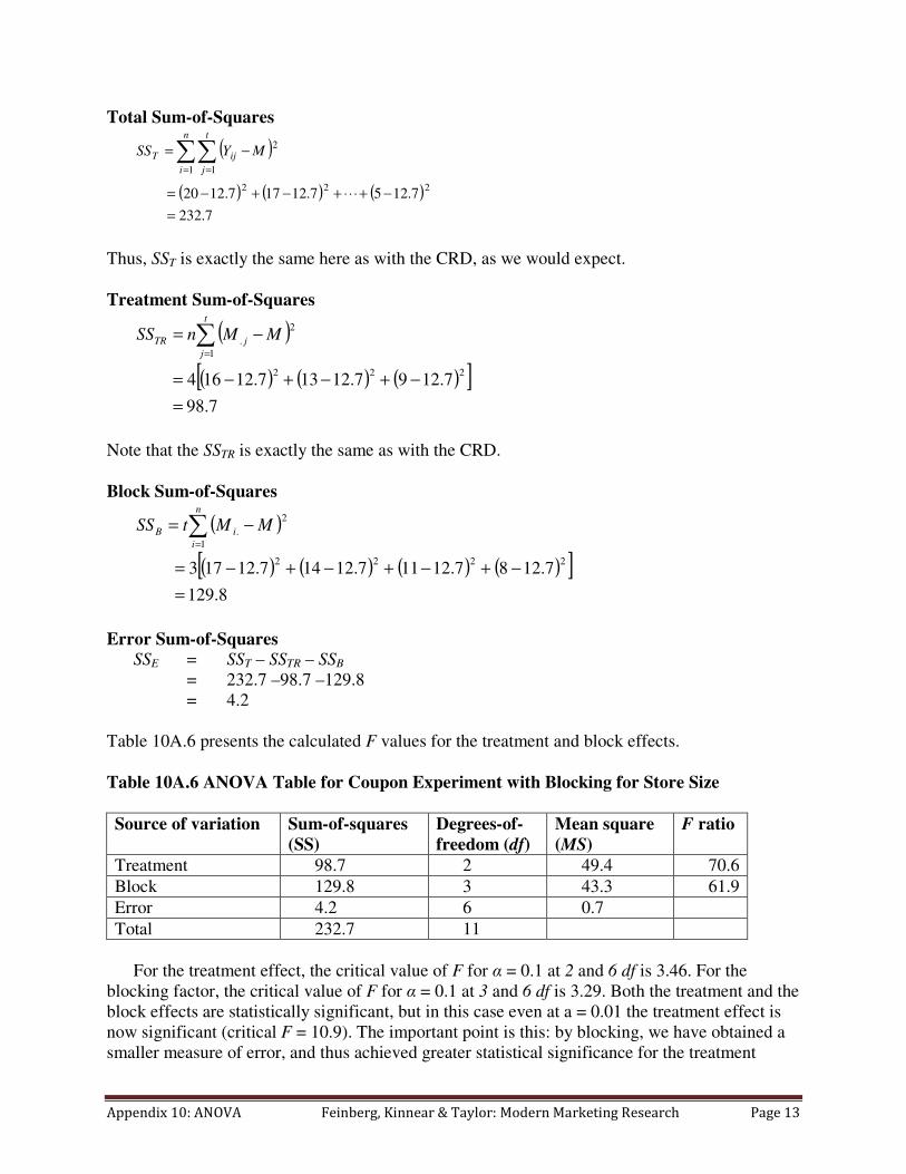
Total Sum-of-Squares

( )

( ) ( ) ( )7.232

7.1257.12177.1220222

1 1

2

=

−+⋅⋅⋅+−+−=

−=∑∑= =

n

i

t

j

ijT MYSS

Thus, SST is exactly the same here as with the CRD, as we would expect.


( )

( ) ( ) ( )[ ]7.98

7.1297.12137.12164222

1

2

.

=

−+−+−=

−= ∑=

t

j

jTR MMnSS

Note that the SSTR is exactly the same as with the CRD.

Block Sum-of-Squares

( )

( ) ( ) ( ) ( )[ ]8.129

7.1287.12117.12147.121732222

1

2

.

=

−+−+−+−=

−= ∑=

n

i

iB MMtSS


SSE = SST – SSTR – SSB

= 232.7 –98.7 –129.8

= 4.2

Table 10A.6 presents the calculated F values for the treatment and block effects.

Table 10A.6 ANOVA Table for Coupon Experiment with Blocking for Store Size

Source of variation Sum-of-squares

(SS)

Degrees-of-

freedom (df)

Mean square

(MS)

F ratio

Treatment 98.7 2 49.4 70.6

Block 129.8 3 43.3 61.9

Error 4.2 6 0.7

Total 232.7 11

For the treatment effect, the critical value of F for α = 0.1 at 2 and 6 df is 3.46. For the

blocking factor, the critical value of F for α = 0.1 at 3 and 6 df is 3.29. Both the treatment and the

block effects are statistically significant, but in this case even at a = 0.01 the treatment effect is

now significant (critical F = 10.9). The important point is this: by blocking, we have obtained a

smaller measure of error, and thus achieved greater statistical significance for the treatment


effect. Note that this does not mean the treatment effect has itself gotten larger; rather, we are

just more certain that it is not merely a stroke of random (misleading) luck. Finally, note that SSB

comes out of the SSE for the CRD; that is,

SSE(with blocking) = SSE(without blocking) – SSB

In our example,

SSE (with blocking) = 134.0 – 129.8 = 4.2

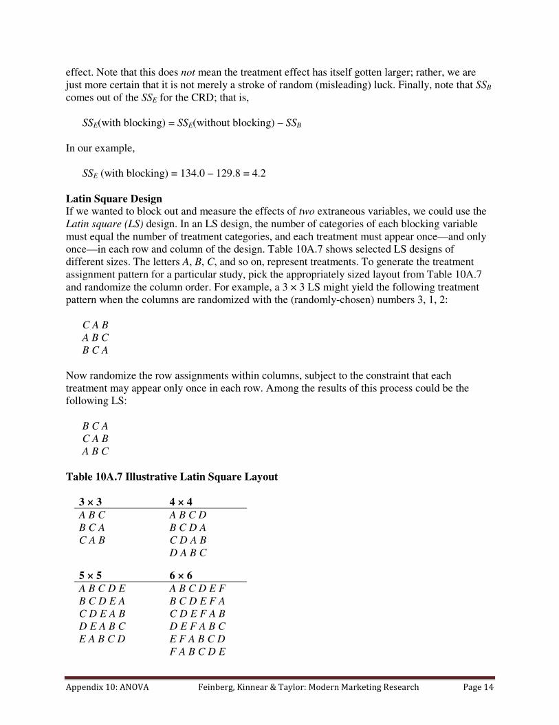
Latin Square Design

If we wanted to block out and measure the effects of two extraneous variables, we could use the

Latin square (LS) design. In an LS design, the number of categories of each blocking variable

must equal the number of treatment categories, and each treatment must appear once—and only

once—in each row and column of the design. Table 10A.7 shows selected LS designs of

different sizes. The letters A, B, C, and so on, represent treatments. To generate the treatment

assignment pattern for a particular study, pick the appropriately sized layout from Table 10A.7

and randomize the column order. For example, a 3 × 3 LS might yield the following treatment

pattern when the columns are randomized with the (randomly-chosen) numbers 3, 1, 2:

C A B

A B C

B C A

Now randomize the row assignments within columns, subject to the constraint that each

treatment may appear only once in each row. Among the results of this process could be the

following LS:

B C A

C A B

A B C

Table 10A.7 Illustrative Latin Square Layout

3 × 3 4 × 4

A B C A B C D

B C A B C D A

C A B C D A B

D A B C

5 × 5 6 × 6

A B C D E A B C D E F

B C D E A B C D E F A

C D E A B C D E F A B

D E A B C D E F A B C

E A B C D E F A B C D

F A B C D E


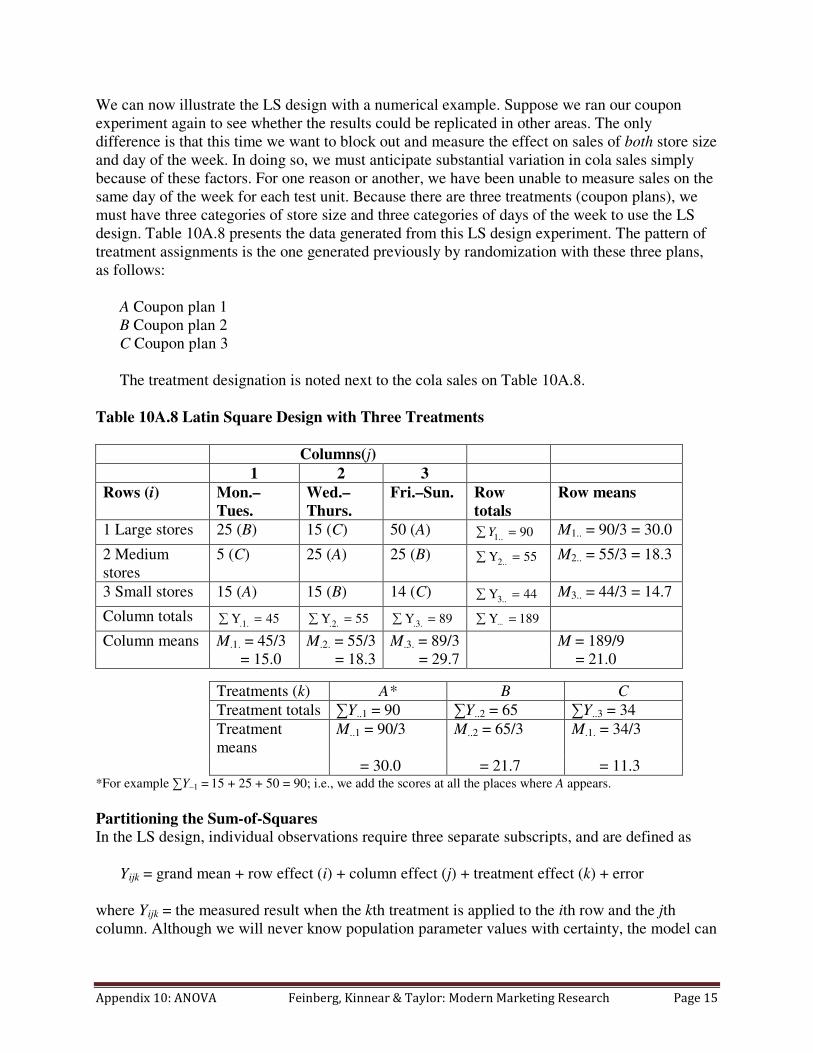
We can now illustrate the LS design with a numerical example. Suppose we ran our coupon

experiment again to see whether the results could be replicated in other areas. The only

difference is that this time we want to block out and measure the effect on sales of both store size

and day of the week. In doing so, we must anticipate substantial variation in cola sales simply

because of these factors. For one reason or another, we have been unable to measure sales on the

same day of the week for each test unit. Because there are three treatments (coupon plans), we

must have three categories of store size and three categories of days of the week to use the LS

design. Table 10A.8 presents the data generated from this LS design experiment. The pattern of

treatment assignments is the one generated previously by randomization with these three plans,

as follows:

A Coupon plan 1

B Coupon plan 2

C Coupon plan 3

The treatment designation is noted next to the cola sales on Table 10A.8.

Table 10A.8 Latin Square Design with Three Treatments

Columns(j)

1 2 3

Rows (i) Mon.–

Tues.

Wed.–

Thurs.

Fri.–Sun. Row

totals

Row means

1 Large stores 25 (B) 15 (C) 50 (A) ∑ = 90..1Y M1.. = 90/3 = 30.0

2 Medium

stores

5 (C) 25 (A) 25 (B) ∑ = 55Y2.. M2.. = 55/3 = 18.3

3 Small stores 15 (A) 15 (B) 14 (C) ∑ = 44Y3.. M3.. = 44/3 = 14.7

Column totals ∑ = 45Y.1. ∑ = 55Y.2. ∑ = 89Y.3. ∑ =⋅⋅⋅ 189Y

Column means M.1. = 45/3 M.2. = 55/3 M.3. = 89/3 M = 189/9

= 15.0 = 18.3 = 29.7 = 21.0

Treatments (k) A* B C

Treatment totals ∑Y..1 = 90 ∑Y..2 = 65 ∑Y..3 = 34

Treatment

means

M..1 = 90/3 M..2 = 65/3 M.1. = 34/3

= 30.0 = 21.7 = 11.3 *For example ∑Y–1 =

15 + 25 + 50 = 90; i.e., we add the scores at all the places where A appears.


In the LS design, individual observations require three separate subscripts, and are defined as

Yijk = grand mean + row effect (i) + column effect (j) + treatment effect (k) + error

where Yijk = the measured result when the kth treatment is applied to the ith row and the jth

column. Although we will never know population parameter values with certainty, the model can


be expressed (using Greek symbols) in those terms as well as

Yijk = µ + αi + βj + τk + Єijk

Because, as always, we will be estimating this model with sample data, we state the model (using

Roman symbols) as

Yijk = M + Ri + Cj + Tk + Eijk

where Ri = the effect of the ith row block (i.e., store size)

Cj = the effect of the jth column block (i.e., day of the week)

Tk =

the effect of the kth treatment (i.e., coupon plan)

Eijk =

the experimental error of the ijk observation

i, j, k = 1,2, …, t where t = the number of treatments

The three effects of interest are:

1. Row effect (i.e., effect of store size) = (Mi.. – M), the difference between the row mean and

the grand mean, adding across all j’s and k’s.

2. Column effect (i.e., effect of the day of the week) = (M.j. – M), the difference between the

column mean and the grand mean, adding across all i’s and k’s.

3. Treatment effect (i.e., effect of coupon plan) = (M..k – M), the difference between the

treatment mean and the grand mean, adding across all i’s and j’s.

We assume that the net effect of each effect is zero (this is taken care of automatically by the

statistical program). That is,

∑∑∑===

===t

k

k

t

j

i

t

i

i TCR

111

0and00

We can then rewrite the equation for our model as

( ) ( ) ( )

erroreffect

treatment

effect

column

effect

row

mean

grand

score

Individual

......

++++=

↓↓↓↓↓↓

+−+−+−+= ijkkji EMMMMMMMijk

Y

We can solve this equation for Eijk to obtain the measurement of error:

Eijk = Yijk – M – (Mi.. – M) – (M.j. – M) – (M..k – M)

= Yijk + 2M – Mi..– M.j. – M..k

This is a complicated procedure, and the student may wonder whether and why it’s

necessary. The key point is this: if both blocking factors are correlated with the dependent

variable, this error measure will be smaller than that obtained with a CRD or RBD that uses only


one blocking factor. Reducing error allows for greater ability to detect the “signal” of the

treatment effect, as represented by its significance level.

If we moved M to the left side, added all these deviations across all rows and columns, and

squared the equation, we would obtain the required SS. The model would then be

SST = SSR + SSC + SSTR + SSE

as yet again all the cross products turn out to be zero. Table 10A.9 shows the ANOVA layout for

an LS design. SSR, SSC, and SSTR each have t – 1 df. With (t)(t) – 1 or t2

– 1 df in the entire

sample, this leaves (t – 1)(t – 2) df for the error term.

Table 10A.9 ANOVA Table for Latin Square Design

Source of

variation

Sum of squares

(SS)

Degrees of

freedom (df)


Between rows SSR t – 1

1−=

t

SSMS R

R E

R

MS

MS

Between

columns

SSC t – 1

1−=

t

SSMS C

C E

C

MS

MS

Between

treatments

SSTR t – 1

1−=

t

SSMS TR

TR E

TR

MS

MS

Error SSE (t – 1) (t – 2)

( )( )21 −−=

tt

SSEMS E

Total SST t2 – 1


We shall now apply the LS design ANOVA to the data in Table 10A.8.


( )

( ) ( ) ( )1302

211421152125222

1 1

2

=

−+⋅⋅⋅+−+−=

−=∑∑= =

t

i

t

j

ijkT MYSS

Row Sum-of-Squares

( )

( ) ( ) ( )[ ]9.383

217.14213.1821303222

1

2..

=

−+⋅⋅⋅+−+−=

−= ∑=

t

i

iR MMtSS


Column Sum-of-Squares

( )

( ) ( ) ( )[ ]9.356

217.29213.1821153222

1

2..

=

−+⋅⋅⋅+−+−=

−= ∑=

t

j

jC MMtSS


( )

( ) ( ) ( )[ ]7.526

213.11217.2121303222

1

2..

=

−+−+−=

−= ∑=

t

i

kTR MMtSS


SSE = SST – SSR – SSC – SSTR

= 1302 – 383.9 – 356.9 – 526.7

= 34.5

Table 10A.10 presents the calculated F values for the treatment and the two blocks. For the

treatment and blocking factors, the critical value of F for α = 0.1 at 2 and 2 df is 9.0. Therefore,

both blocking factors and the treatment are significant. Note that none of these effects would

have been significant at α = 0.05, as the critical F is 19.0. If we had used a CRD or blocked with

just one of our two blocking factors in an RBD, the treatment effect would not have been

significant, even at a = 0.1. This is so because the SSR and SSC would be added back into the LS

design SSE to give the SSE for the CRD. As for the RBD, either SSR or SSC would be added back

to the LS design SSE to give the SSE for the RBD. In either instance, the SSR or SSC is large

enough to render the calculated F ratio nonsignificant at α = 0.1. Here, we needed two blocking

factors to find in favor of a significant treatment effect. The value of blocking in marketing

experiments should be clear. Again, note that we must look closely at the data to see that

treatment A is the best coupon plan; the ANOVA results alone will not make this determination

for us.

Table 10A.10 ANOVA Table for Coupon Experiment with 3 x 3 Latin Square Design

Source of

variation

Sum-of-

squares (SS)

Degrees–of-

freedom (df)

Mean square

(MS)

F ratio

Row effect

(store size)

383.9 2 192.0 11.1

Column effect

(days of week)

356.9 2 178.5 10.3

Treatment 526.7 2 263.4 15.2

Error 34.5 2 17.3

Total 1302.0 8 Note: nij = 2 for all i’s and j’s.


Factorial Design

In a factorial design (FD), we measure the effects of two or more independent variables and their

interactions. Suppose that in our coupon experiment we are interested not only in the effect of

coupon plans, but also in the effect of the media plans that support the coupon plans. Table

10A.11 presents data stemming from such an experiment. You should recognize these as the data

we used in Table 10A.1 for our CRD. All we have done here is regroup the data and present

them as if they came from an FD.

Table 10A.11 A 2× 3 Factorial Design with Media Plans and Coupon Plans as Independent

Variables

Coupon plans (j )

B1 B2 B3 Media

totals

Media means

Media

plans (i) A1 20 17 14 ∑ = 93Y ..1 M1.. =

93/6 = 15.5

18 14 10

A2 15 13 7 ∑ = 59Y2.. M2.. = 59/6 = 9.8

11 8 5

Coupon

totals

∑ = 64Y.1. ∑ = 52Y.2. ∑ = 36Y.3. ∑ = 152...Y

Coupon

means

M.1. = 64/4

= 16

M.2. = 52/4 =

13

M.3. = 36/4

= 9

M = 12.7

Treatment

cell (ij)

A1B1 A1B2 A1B3 A2B1 A2B2 A2B3

Cell total ∑ = 38Y11. ∑ = 31Y12. ∑ = 24Y13. ∑ = 26Y21. ∑ = 21Y22. ∑ = 12Y23.

Cell mean M11. = 38/2 M12. = 31/2 M13. = 24/2 M21. = 26/2 M22. = 21/2 M23. = 12/2

= 19 =15.5 =12 = 13 = 10.5 = 6

Note: nij = 2 for all i’s and j’s.


In the FD with two independent variables, we define an individual observation as

Yijk = grand mean + effect of treatment A + effect of treatment B + interaction effect AB +

error

where Yijk = the kth observation on the ith level of A and the jth level of B.

For example, here

Y111 = 20 and Y231 =

7

In population parameter terms, the model is

Yijk = µ + αi + βj + (αβ)ij + Єijk


Again, as always, we will be estimating this model with sample data, and we write

Yijk = M + Ai + Bj + (AB)ij + E ijk

where Ai =

the effect of the ith level of A (media plan), i = 1; . ..; a,

where a is the number of levels in A

Bj = the effect of the ith level of B (coupon plan), j = 1; ... ; b,

where b is the number of levels in B

(AB)ij = the effect of the interaction of the ith level of A and the jth level of B

Eijk = the error of the kth observation in the ith level of A and the jth level of

B, that is, the ij cell

In our example nij = 2 for all ij cells. The four effects of interest are:

1. Ai effect (i.e., media plan) = (Mi.. – M), the difference between the row mean and the grand

mean.

2. Bj effect (i.e., coupon plan) = (M.j. – M), the difference between the column mean and the

grand mean.

3. Error = (Yijk – Mij.), the difference between an individual observation and the cell mean to

which it belongs. That is, the only differences within a cell should be due to randomness

(error).

4. Interaction effect (AB)ij = any remaining variation in the data after main effects and error

have been removed.

We can now rewrite the equation for our model as

Yijk = M + (Mi.. – M)+ (M.j. – M) + (AB)ij + (Yijk – Mij.)

and solve for the interaction term, (AB)ij:

AB = Yijk – M – (Mi.. – M) – (M.j. – M) – (Yijk – Mij.)

= Yijk – M – Mi.. + M – M.j. + M – Yijk + Mij.

= M + Mij. – Mij. – M.j.

In our example,

(AB)11 = 12.7 + 19 – 15.5 – 16 = 0.2

and

(AB)23 = 12.7 + 6 – 9.8 – 9 = –0.1


Results like this suggest that there is little interaction in the data, although we have not yet

performed any statistical tests to confirm this informal observation. We may now rewrite our

equation as

Yijk = M + (Mi.. – M) + (M.j. – M) + (M + Mij. – Mi.. – M.j.) + (Yijk – Mij.)

If we moved M to the left side, added all the deviations across all scores k in all ij cells, and

squared the equation, we would obtain the required SS. The model would then be

SST = SSTRA + SSTRB + SSINT(AB) + SSE

where SSTRA = sum-of-squares of treatment A

SSTRB = sum-of-squares of treatment B

SSINT (AB) = sum-of-squares for interaction of A and B

This result occurs because all the cross-products are, as in our other ANOVA examples, zero.

Table 10A.12 shows the ANOVA layout for a two-factor FD. Each factor has one degree-of-

freedom less than its number of categories, and the interaction term has (a – 1) (b – 1) df. With

abn – 1 df in the whole sample, this leaves ab(n – 1) for the error term.

Table 10A.12 ANOVA Table for a Two-Factor Factorial Design

Source of variation Sum of

squares (SS)

Degrees of

freedom (df)


Treatment A SSTRA a – 1

1−=

a

SSMS TRA

TRA E

TRA

MS

MS

Treatment B SSTRB b – 1

1−=

b

SSMS TRB

TRB E

TRB

MS

MS

Interaction AB SSINT(AB) (a – 1)(b – 1)

1)1)( −−=

(ba

SSMS

INT(AB)

INT(AB) E

INT(AB)

MS

MS

Error SSE ab(n – 1)

1)( −=

nab

SSMS E

E

Total SST abn – 1


Now let us apply the FD to the data in Table 10A.11.


( )

( ) ( ) ( )7.232

7.1257.12177.1220222

1 1 1

2

=

−+⋅⋅⋅+−+−=

−=∑∑∑= = =

a

i

b

j

n

k

jkT MYiSS


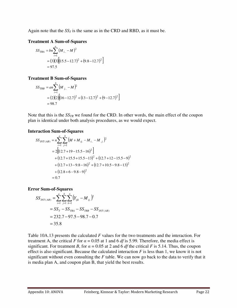
Again note that the SST is the same as in the CRD and RBD, as it must be.

Treatment A Sum-of-Squares

( )

( )( ) ( ) ( )[ ]5.97

7.128.97.125.153322

1

2..

=

−+−=

−= ∑=

a

i

iTRA MMbnSS

Treatment B Sum-of-Squares

( )

( )( ) ( ) ( ) ( )[ ]7.98

7.1297.12137.121622222

1

2..

=

−+−+−=

−= ∑=

b

i

jTRB MManSS

Note that this is the SSTR we found for the CRD. In other words, the main effect of the coupon

plan is identical under both analysis procedures, as we would expect.

Interaction Sum-of-Squares

( )

( )[ ]( ) ( )( ) ( )( )7.0

98.968.12

138.95.107.12168.9137.12

95.15127.12135.155.157.12

165.15197.122

2

22

22

2

1 1

2.....)(

=

−−++

−−++−−++

−−++−+++

−−+=

−−+= ∑∑= =

a

i

b

j

jiijABINT MMMMnSS


( )

8.35

7.07.985.977.232

)(

1 1 1

2

.)(

=

−−−=

−−−=

−=∑∑∑= = =

ABINTTRBTRAT

a

i

b

j

n

k

ijijkABINT

SSSSSSSS

MYSS

Table 10A.13 presents the calculated F values for the two treatments and the interaction. For

treatment A, the critical F for α = 0.05 at 1 and 6 df is 5.99. Therefore, the media effect is

significant. For treatment B, for α = 0.05 at 2 and 6 df the critical F is 5.14. Thus, the coupon

effect is also significant. Because the calculated interaction F is less than 1, we know it is not

significant without even consulting the F table. We can now go back to the data to verify that it

is media plan A, and coupon plan B, that yield the best results.


Table 10A.13 ANOVA Table for Media and Coupon Experiment Using a Two-Factor

2 × 3 Factorial Design

Source of

variation

Sum-of-

squares (SS)

Degrees-of-

freedom (df)

Mean square

(MS)

F ratio

Treatment A

(media)

97.5 1 97.5 16.3

Treatment B

(coupon)

98.7 2 49.4 8.2

Interaction

(AB)

0.7 2 0.4 0.1

Error 35.8 6 6.0

Total 232.7 11

This two-factor ANOVA is usually referred to as “two-way” ANOVA. The factorial

procedure can be extended to any number (N) of independent variables, and is often called “N-

way” ANOVA. The calculations for an ANOVA greater than two-way are too complex to

present here, although they are analogous to those carried out for the two-way ANOVA design.

The analysis of such an experiment is, however, easily handled by statistical programs. In any

event, the principles underlying all complex ANOVA designs are the same as those developed

here.

Summary of Appendix

1. ANOVA involves the calculation and comparison of different variance estimates, SS/df.

2. The fixed-effects model allows inferences only about the different treatments actually used.

It is, among the various ANOVA designs, the one most directly relevant in marketing.

3. In ANOVA, an effect is defined as a difference in treatment mean from the grand mean.

4. Experimental error is the difference between an individual score and the treatment group

mean to which the score belongs.

5. ANOVA is carried out by partitioning the SST into SSTR and SSE and dividing each of these

by their relevant degrees-of-freedom to yield an estimate of treatment and error variances,

called the mean squares (MSTR and MSE). That is, the one-way ANOVA model is partitioned

as follows: SST = SSTR + SSE.

6. The relevant statistic for a significance test is the F statistic, where F = MSTR/MSE.

7. The CRD (completely randomized design) measures the effect of one independent variable

without statistical control of extraneous variation. Its basic composition is SST = SSTR + SSE.

8. The RBD (randomized block design) measures the effect of one independent variable with

statistical control of one extraneous factor. Its basic composition is SST = SSTR + SSB + SSE.

9. The LS (Latin square) design measures the effect of one independent variable with statistical

control of two extraneous factors. Its basic composition is SST = SSR + SSC + SSTR + SSE.

10. The FD (factorial design) measures the main and interaction effects of two or more

independent variables. Its basic composition for a two-way ANOVA is SST = SSTRA + SSTRB +

SSINT(AB) + SSE.

Documents

APPENDIX 10: ANALYSIS OF VARIANCE (ANOVA) Modern Marketing ...webuser.bus.umich.edu/feinf/modernmarketingresearch/Chapter_10... · Appendix 10: ANOVA Feinberg, Kinnear & Taylor: Modern