AP Statistics 2007 Free-Response Questions€¦ · 2007 AP® STATISTICS FREE-RESPONSE QUESTIONS -3- Formulas (I) Descriptive Statistics x xi n = ∑ s n x = − ∑ xi −x 1 1 di2

AP® Statistics 2007 Free-Response Questions

The College Board: Connecting Students to College Success

The College Board is a not-for-profit membership association whose mission is to connect students to college success and opportunity. Founded in 1900, the association is composed of more than 5,000 schools, colleges, universities, and other educational organizations. Each year, the College Board serves seven million students and their parents, 23,000 high schools, and 3,500 colleges through major programs and services in college admissions, guidance, assessment, financial aid, enrollment, and teaching and learning. Among its best-known programs are the SAT®, the PSAT/NMSQT®, and the Advanced Placement Program® (AP®). The College Board is committed to the principles of excellence and equity, and that commitment is embodied in all of its programs, services, activities, and concerns.

© 2007 The College Board. All rights reserved. College Board, Advanced Placement Program, AP, AP Central, SAT, and the acorn logo are registered trademarks of the College Board. PSAT/NMSQT is a registered trademark of the College Board and National Merit Scholarship Corporation. Permission to use copyrighted College Board materials may be requested online at: www.collegeboard.com/inquiry/cbpermit.html. Visit the College Board on the Web: www.collegeboard.com. AP Central is the official online home for the AP Program: apcentral.collegeboard.com.

2007 AP® STATISTICS FREE-RESPONSE QUESTIONS

-2-

Formulas begin on page 3. Questions begin on page 6. Tables begin on page 12.


-3-

Formulas (I) Descriptive Statistics

xxi

n=∑

s n xi xx = − −∑11

2d i

sn s n s

n np =− + −

− + −

121 2

22

1 2

1 1

1 1

d i d id i d i

y b b x= +0 1

bx x y y

x x

i i

i1 2

=− −

−

∑

∑

d id id i

b y b x0 1= −

r nx x

sy y

si

x

i

y= −

− −FHG

IKJ∑FHG

IKJ

11

b rssy

x1 =

s

y yn

x xb

i i

i1

2

2

2=

−−

−

∑

∑

d i

d i


-4-

(II) Probability

P A B P A P B P A B( ) ( ) ( ) ( )∪ = + − ∩

P A B P A BP B( )

( )( )

= ∩

E X x xi pi( ) = = ∑μ

Var( )X x pix i x= = −∑s 2 2μd i

If X has a binomial distribution with parameters n and p , then:

P X knk

pk p n k( ) ( )= = − −FHG

IKJ 1

μ x np=

s x np p= −( )1

μ p p=

s( )

pp p

n=−1

If x is the mean of a random sample of size n from an infinite population with mean μ and standard deviation s, then:

μ μx =

s sx n

=


-5-

(III) Inferential Statistics

Standardized test statistic:statistic parameter

standard deviation of statistic-

Confidence interval: statistic critical value standard deviation of statistic± ( ) ( )∑

Single-Sample

Statistic Standard Deviation of Statistic

Sample Mean

σn

Sample Proportion

p pn

( )1 −

Two-Sample

Statistic Standard Deviation of Statistic

Difference of sample means

σ σ12

1

22

2n n+

Special case when σ σ1 2=

σ 1 1

1 2n n+

Difference of

sample proportions

p p

np p

n1 1

1

2 2

2

1 1( ) ( )−+

−

Special case when p p1 2=

p p1−b g 1 1

1 2n n+

Chi-square test statisticobserved expected

expected=

−∑ a f2


© 2007 The College Board. All rights reserved. Visit apcentral.collegeboard.com (for AP professionals) and www.collegeboard.com/apstudents (for students and parents).

GO ON TO THE NEXT PAGE. -6-

STATISTICS SECTION II

Part A Questions 1-5

Spend about 65 minutes on this part of the exam. Percent of Section II grade—75

Directions: Show all your work. Indicate clearly the methods you use, because you will be graded on the correctness of your methods as well as on the accuracy and completeness of your results and explanations. 1. The department of agriculture at a university was interested in determining whether a preservative was effective

in reducing discoloration in frozen strawberries. A sample of 50 ripe strawberries was prepared for freezing. Then the sample was randomly divided into two groups of 25 strawberries each. Each strawberry was placed into a small plastic bag.

The 25 bags in the control group were sealed. The preservative was added to the 25 bags containing strawberries in the treatment group, and then those bags were sealed. All bags were stored at 0 C� for a period of 6 months. At the end of this time, after the strawberries were thawed, a technician rated each strawberry’s discoloration from 1 to 10, with a low score indicating little discoloration.

The dotplots below show the distributions of discoloration rating for the control and treatment groups.

(a) The standard deviation of ratings for the control group is 2.141. Explain how this value summarizes variability in the control group.

(b) Based on the dotplots, comment on the effectiveness of the preservative in lowering the amount of discoloration in strawberries. (No calculations are necessary.)

(c) Researchers at the university decided to calculate a 95 percent confidence interval for the difference in mean discoloration rating between strawberries that were not treated with preservative and those that were treated with preservative. The confidence interval they obtained was (0.16, 2.72). Assume that the conditions necessary for the t-confidence interval are met.

Based on the confidence interval, comment on whether there would be a difference in the population mean discoloration ratings for the treated and untreated strawberries.




2. As dogs age, diminished joint and hip health may lead to joint pain and thus reduce a dog’s activity level. Such a reduction in activity can lead to other health concerns such as weight gain and lethargy due to lack of exercise. A study is to be conducted to see which of two dietary supplements, glucosamine or chondroitin, is more effective in promoting joint and hip health and reducing the onset of canine osteoarthritis. Researchers will randomly select a total of 300 dogs from ten different large veterinary practices around the country. All of the dogs are more than 6 years old, and their owners have given consent to participate in the study. Changes in joint and hip health will be evaluated after 6 months of treatment.

(a) What would be an advantage to adding a control group in the design of this study?

(b) Assuming a control group is added to the other two groups in the study, explain how you would assign the 300 dogs to these three groups for a completely randomized design.

(c) Rather than using a completely randomized design, one group of researchers proposes blocking on clinics, and another group of researchers proposes blocking on breed of dog. How would you decide which one of these two variables to use as a blocking variable?

3. Big Town Fisheries recently stocked a new lake in a city park with 2,000 fish of various sizes. The distribution

of the lengths of these fish is approximately normal.

(a) Big Town Fisheries claims that the mean length of the fish is 8 inches. If the claim is true, which of the following would be more likely?

• A random sample of 15 fish having a mean length that is greater than 10 inches

or • A random sample of 50 fish having a mean length that is greater than 10 inches

Justify your answer.

(b) Suppose the standard deviation of the sampling distribution of the sample mean for random samples of size 50 is 0.3 inch. If the mean length of the fish is 8 inches, use the normal distribution to compute the probability that a random sample of 50 fish will have a mean length less than 7.5 inches.

(c) Suppose the distribution of fish lengths in this lake was nonnormal but had the same mean and standard deviation. Would it still be appropriate to use the normal distribution to compute the probability in part (b) ? Justify your answer.




4. Investigators at the U.S. Department of Agriculture wished to compare methods of determining the level of E. coli bacteria contamination in beef. Two different methods (A and B) of determining the level of contamination were used on each of ten randomly selected specimens of a certain type of beef. The data obtained, in millimicrobes/liter of ground beef, for each of the methods are shown in the table below.

Specimen

1 2 3 4 5 6 7 8 9 10

A 22.7 23.6 24.0 27.1 27.4 27.8 34.4 35.2 40.4 46.8

Method B 23.0 23.1 23.7 26.5 26.6 27.1 33.2 35.0 40.5 47.8

Is there a significant difference in the mean amount of E. coli bacteria detected by the two methods for this

type of beef? Provide a statistical justification to support your answer.




5. Researchers want to determine whether drivers are significantly more distracted while driving when using a cell phone than when talking to a passenger in the car. In a study involving 48 people, 24 people were randomly assigned to drive in a driving simulator while using a cell phone. The remaining 24 were assigned to drive in the driving simulator while talking to a passenger in the simulator. Part of the driving simulation for both groups involved asking drivers to exit the freeway at a particular exit. In the study, 7 of the 24 cell phone users missed the exit, while 2 of the 24 talking to a passenger missed the exit.

(a) Would this study be classified as an experiment or an observational study? Provide an explanation to support your answer.

(b) State the null and alternative hypotheses of interest to the researchers.

(c) One test of significance that you might consider using to answer the researchers’ question is a two-sample z-test. State the conditions required for this test to be appropriate. Then comment on whether each condition is met.

(d) Using an advanced statistical method for small samples to test the hypotheses in part (b), the researchers report a p-value of 0.0683. Interpret, in everyday language, what this p-value measures in the context of this study and state what conclusion should be made based on this p-value.




STATISTICS SECTION II

Part B Question 6

Spend about 25 minutes on this part of the exam. Percent of Section II grade—25

Directions: Show all your work. Indicate clearly the methods you use, because you will be graded on the correctness of your methods as well as on the accuracy and completeness of your results and explanations. 6. A study was designed to explore subjects’ ability to judge the distance between two objects placed in a dimly lit

room. The researcher suspected that the subjects would generally overestimate the distance between the objects in the room and that this overestimation would increase the farther apart the objects were.

The two objects were placed at random locations in the room before a subject estimated the distance (in feet) between those two objects. After each subject estimated the distance, the locations of the objects were rerandomized before the next subject viewed the room.

After data were collected for 40 subjects, two linear models were fit in an attempt to describe the relationship between the subjects’ perceived distances (y) and the actual distance, in feet, between the two objects.

Model 1: ˆ 0.238 1.080 (actual distance)= +y �

The standard errors of the estimated coefficients for Model 1 are 0.260 and 0.118, respectively.

Model 2: ˆ 1.102 (actual distance)=y �

The standard error of the estimated coefficient for Model 2 is 0.393.

(a) Provide an interpretation in context for the estimated slope in Model 1.

(b) Explain why the researcher might prefer Model 2 to Model 1 in this context.

(c) Using Model 2, test the researcher’s hypothesis that in dim light participants overestimate the distance, with the overestimate increasing as the actual distance increases. (Assume appropriate conditions for inference are met.)

The researchers also wanted to explore whether the performance on this task differed between subjects who wear contact lenses and subjects who do not wear contact lenses. A new variable was created to indicate whether or not a subject wears contact lenses. The data for this variable were coded numerically (1 = contact wearer, 0 = noncontact wearer), and this new variable, named “contact,” was included in the following model.

Model 3: ( )ˆ 1.05 (actual distance) 0.12 (contact) actual distance= +y � � �

The standard errors of the estimated coefficients for Model 3 are 0.357 and 0.032, respectively.



-11-

(d) Using Model 3, sketch the estimated regression model for contact wearers and the estimated regression model for noncontact wearers on the grid below.

(e) In the context of this study, provide an interpretation of the estimated coefficients for Model 3.

STOP

END OF EXAM


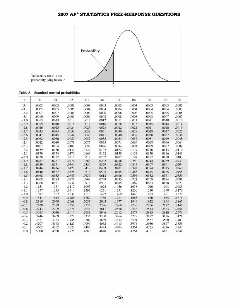
-12-

Probability

z

Table A Standard normal probabilities

z .00 .01 .02 .03 .04 .05 .06 .07 .08 .09 –3.4 .0003 .0003 .0003 .0003 .0003 .0003 .0003 .0003 .0003 .0002 –3.3 .0005 .0005 .0005 .0004 .0004 .0004 .0004 .0004 .0004 .0003 –3.2 .0007 .0007 .0006 .0006 .0006 .0006 .0006 .0005 .0005 .0005 –3.1 .0010 .0009 .0009 .0009 .0008 .0008 .0008 .0008 .0007 .0007 –3.0 .0013 .0013 .0013 .0012 .0012 .0011 .0011 .0011 .0010 .0010 –2.9 .0019 .0018 .0018 .0017 .0016 .0016 .0015 .0015 .0014 .0014 –2.8 .0026 .0025 .0024 .0023 .0023 .0022 .0021 .0021 .0020 .0019 –2.7 .0035 .0034 .0033 .0032 .0031 .0030 .0029 .0028 .0027 .0026 –2.6 .0047 .0045 .0044 .0043 .0041 .0040 .0039 .0038 .0037 .0036 –2.5 .0062 .0060 .0059 .0057 .0055 .0054 .0052 .0051 .0049 .0048 –2.4 .0082 .0080 .0078 .0075 .0073 .0071 .0069 .0068 .0066 .0064 –2.3 .0107 .0104 .0102 .0099 .0096 .0094 .0091 .0089 .0087 .0084 –2.2 .0139 .0136 .0132 .0129 .0125 .0122 .0119 .0116 .0113 .0110 –2.1 .0179 .0174 .0170 .0166 .0162 .0158 .0154 .0150 .0146 .0143 –2.0 .0228 .0222 .0217 .0212 .0207 .0202 .0197 .0192 .0188 .0183 –1.9 .0287 .0281 .0274 .0268 .0262 .0256 .0250 .0244 .0239 .0233 –1.8 .0359 .0351 .0344 .0336 .0329 .0322 .0314 .0307 .0301 .0294 –1.7 .0446 .0436 .0427 .0418 .0409 .0401 .0392 .0384 .0375 .0367 –1.6 .0548 .0537 .0526 .0516 .0505 .0495 .0485 .0475 .0465 .0455 –1.5 .0668 .0655 .0643 .0630 .0618 .0606 .0594 .0582 .0571 .0559 –1.4 .0808 .0793 .0778 .0764 .0749 .0735 .0721 .0708 .0694 .0681 –1.3 .0968 .0951 .0934 .0918 .0901 .0885 .0869 .0853 .0838 .0823 –1.2 .1151 .1131 .1112 .1093 .1075 .1056 .1038 .1020 .1003 .0985 –1.1 .1357 .1335 .1314 .1292 .1271 .1251 .1230 .1210 .1190 .1170 –1.0 .1587 .1562 .1539 .1515 .1492 .1469 .1446 .1423 .1401 .1379 –0.9 .1841 .1814 .1788 .1762 .1736 .1711 .1685 .1660 .1635 .1611 –0.8 .2119 .2090 .2061 .2033 .2005 .1977 .1949 .1922 .1894 .1867 –0.7 .2420 .2389 .2358 .2327 .2296 .2266 .2236 .2206 .2177 .2148 –0.6 .2743 .2709 .2676 .2643 .2611 .2578 .2546 .2514 .2483 .2451 –0.5 .3085 .3050 .3015 .2981 .2946 .2912 .2877 .2843 .2810 .2776 –0.4 .3446 .3409 .3372 .3336 .3300 .3264 .3228 .3192 .3156 .3121 –0.3 .3821 .3783 .3745 .3707 .3669 .3632 .3594 .3557 .3520 .3483 –0.2 .4207 .4168 .4129 .4090 .4052 .4013 .3974 .3936 .3897 .3859 –0.1 .4602 .4562 .4522 .4483 .4443 .4404 .4364 .4325 .4286 .4247 –0.0 .5000 .4960 .4920 .4880 .4840 .4801 .4761 .4721 .4681 .4641

Table entry for z is the probability lying below z.


-13-

Probability

z

Table A (Continued)

z .00 .01 .02 .03 .04 .05 .06 .07 .08 .09 0.0 .5000 .5040 .5080 .5120 .5160 .5199 .5239 .5279 .5319 .5359 0.1 .5398 .5438 .5478 .5517 .5557 .5596 .5636 .5675 .5714 .5753 0.2 .5793 .5832 .5871 .5910 .5948 .5987 .6026 .6064 .6103 .6141 0.3 .6179 .6217 .6255 .6293 .6331 .6368 .6406 .6443 .6480 .6517 0.4 .6554 .6591 .6628 .6664 .6700 .6736 .6772 .6808 .6844 .6879 0.5 .6915 .6950 .6985 .7019 .7054 .7088 .7123 .7157 .7190 .7224 0.6 .7257 .7291 .7324 .7357 .7389 .7422 .7454 .7486 .7517 .7549 0.7 .7580 .7611 .7642 .7673 .7704 .7734 .7764 .7794 .7823 .7852 0.8 .7881 .7910 .7939 .7967 .7995 .8023 .8051 .8078 .8106 .8133 0.9 .8159 .8186 .8212 .8238 .8264 .8289 .8315 .8340 .8365 .8389 1.0 .8413 .8438 .8461 .8485 .8508 .8531 .8554 .8577 .8599 .8621 1.1 .8643 .8665 .8686 .8708 .8729 .8749 .8770 .8790 .8810 .8830 1.2 .8849 .8869 .8888 .8907 .8925 .8944 .8962 .8980 .8997 .9015 1.3 .9032 .9049 .9066 .9082 .9099 .9115 .9131 .9147 .9162 .9177 1.4 .9192 .9207 .9222 .9236 .9251 .9265 .9279 .9292 .9306 .9319 1.5 .9332 .9345 .9357 .9370 .9382 .9394 .9406 .9418 .9429 .9441 1.6 .9452 .9463 .9474 .9484 .9495 .9505 .9515 .9525 .9535 .9545 1.7 .9554 .9564 .9573 .9582 .9591 .9599 .9608 .9616 .9625 .9633 1.8 .9641 .9649 .9656 .9664 .9671 .9678 .9686 .9693 .9699 .9706 1.9 .9713 .9719 .9726 .9732 .9738 .9744 .9750 .9756 .9761 .9767 2.0 .9772 .9778 .9783 .9788 .9793 .9798 .9803 .9808 .9812 .9817 2.1 .9821 .9826 .9830 .9834 .9838 .9842 .9846 .9850 .9854 .9857 2.2 .9861 .9864 .9868 .9871 .9875 .9878 .9881 .9884 .9887 .9890 2.3 .9893 .9896 .9898 .9901 .9904 .9906 .9909 .9911 .9913 .9916 2.4 .9918 .9920 .9922 .9925 .9927 .9929 .9931 .9932 .9934 .9936 2.5 .9938 .9940 .9941 .9943 .9945 .9946 .9948 .9949 .9951 .9952 2.6 .9953 .9955 .9956 .9957 .9959 .9960 .9961 .9962 .9963 .9964 2.7 .9965 .9966 .9967 .9968 .9969 .9970 .9971 .9972 .9973 .9974 2.8 .9974 .9975 .9976 .9977 .9977 .9978 .9979 .9979 .9980 .9981 2.9 .9981 .9982 .9982 .9983 .9984 .9984 .9985 .9985 .9986 .9986 3.0 .9987 .9987 .9987 .9988 .9988 .9989 .9989 .9989 .9990 .9990 3.1 .9990 .9991 .9991 .9991 .9992 .9992 .9992 .9992 .9993 .9993 3.2 .9993 .9993 .9994 .9994 .9994 .9994 .9994 .9995 .9995 .9995 3.3 .9995 .9995 .9995 .9996 .9996 .9996 .9996 .9996 .9996 .9997 3.4 .9997 .9997 .9997 .9997 .9997 .9997 .9997 .9997 .9997 .9998

Table entry for z is the probability lying below z.


-14-

Probability p

t*

Table B t distribution critical values

Tail probability p

df .25 .20 .15 .10 .05 .025 .02 .01 .005 .0025 .001 .0005

1 1.000 1.376 1.963 3.078 6.314 12.71 15.89 31.82 63.66 127.3 318.3 636.6 2 .816 1.061 1.386 1.886 2.920 4.303 4.849 6.965 9.925 14.09 22.33 31.60 3 .765 .978 1.250 1.638 2.353 3.182 3.482 4.541 5.841 7.453 10.21 12.92 4 .741 .941 1.190 1.533 2.132 2.776 2.999 3.747 4.604 5.598 7.173 8.610 5 .727 .920 1.156 1.476 2.015 2.571 2.757 3.365 4.032 4.773 5.893 6.869 6 .718 .906 1.134 1.440 1.943 2.447 2.612 3.143 3.707 4.317 5.208 5.959 7 .711 .896 1.119 1.415 1.895 2.365 2.517 2.998 3.499 4.029 4.785 5.408 8 .706 .889 1.108 1.397 1.860 2.306 2.449 2.896 3.355 3.833 4.501 5.041 9 .703 .883 1.100 1.383 1.833 2.262 2.398 2.821 3.250 3.690 4.297 4.781

10 .700 .879 1.093 1.372 1.812 2.228 2.359 2.764 3.169 3.581 4.144 4.587 11 .697 .876 1.088 1.363 1.796 2.201 2.328 2.718 3.106 3.497 4.025 4.437 12 .695 .873 1.083 1.356 1.782 2.179 2.303 2.681 3.055 3.428 3.930 4.318 13 .694 .870 1.079 1.350 1.771 2.160 2.282 2.650 3.012 3.372 3.852 4.221 14 .692 .868 1.076 1.345 1.761 2.145 2.264 2.624 2.977 3.326 3.787 4.140 15 .691 .866 1.074 1.341 1.753 2.131 2.249 2.602 2.947 3.286 3.733 4.073 16 .690 .865 1.071 1.337 1.746 2.120 2.235 2.583 2.921 3.252 3.686 4.015 17 .689 .863 1.069 1.333 1.740 2.110 2.224 2.567 2.898 3.222 3.646 3.965 18 .688 .862 1.067 1.330 1.734 2.101 2.214 2.552 2.878 3.197 3.611 3.922 19 .688 .861 1.066 1.328 1.729 2.093 2.205 2.539 2.861 3.174 3.579 3.883 20 .687 .860 1.064 1.325 1.725 2.086 2.197 2.528 2.845 3.153 3.552 3.850 21 .686 .859 1.063 1.323 1.721 2.080 2.189 2.518 2.831 3.135 3.527 3.819 22 .686 .858 1.061 1.321 1.717 2.074 2.183 2.508 2.819 3.119 3.505 3.792 23 .685 .858 1.060 1.319 1.714 2.069 2.177 2.500 2.807 3.104 3.485 3.768 24 .685 .857 1.059 1.318 1.711 2.064 2.172 2.492 2.797 3.091 3.467 3.745 25 .684 .856 1.058 1.316 1.708 2.060 2.167 2.485 2.787 3.078 3.450 3.725 26 .684 .856 1.058 1.315 1.706 2.056 2.162 2.479 2.779 3.067 3.435 3.707 27 .684 .855 1.057 1.314 1.703 2.052 2.158 2.473 2.771 3.057 3.421 3.690 28 .683 .855 1.056 1.313 1.701 2.048 2.154 2.467 2.763 3.047 3.408 3.674 29 .683 .854 1.055 1.311 1.699 2.045 2.150 2.462 2.756 3.038 3.396 3.659 30 .683 .854 1.055 1.310 1.697 2.042 2.147 2.457 2.750 3.030 3.385 3.646 40 .681 .851 1.050 1.303 1.684 2.021 2.123 2.423 2.704 2.971 3.307 3.551 50 .679 .849 1.047 1.299 1.676 2.009 2.109 2.403 2.678 2.937 3.261 3.496 60 .679 .848 1.045 1.296 1.671 2.000 2.099 2.390 2.660 2.915 3.232 3.460 80 .678 .846 1.043 1.292 1.664 1.990 2.088 2.374 2.639 2.887 3.195 3.416

100 .677 .845 1.042 1.290 1.660 1.984 2.081 2.364 2.626 2.871 3.174 3.390 1000 .675 .842 1.037 1.282 1.646 1.962 2.056 2.330 2.581 2.813 3.098 3.300

� .674 .841 1.036 1.282 1.645 1.960 2.054 2.326 2.576 2.807 3.091 3.291

50% 60% 70% 80% 90% 95% 96% 98% 99% 99.5% 99.8% 99.9%

Confidence level C

Table entry for p and C is the point t* with probability p lying above it and probability C lying between −t * and t*.


-15-

Probability p

(χ2)

Table C χ 2 critical values Tail probability p

df .25 .20 .15 .10 .05 .025 .02 .01 .005 .0025 .001 .0005

1 1.32 1.64 2.07 2.71 3.84 5.02 5.41 6.63 7.88 9.14 10.83 12.12 2 2.77 3.22 3.79 4.61 5.99 7.38 7.82 9.21 10.60 11.98 13.82 15.20 3 4.11 4.64 5.32 6.25 7.81 9.35 9.84 11.34 12.84 14.32 16.27 17.73 4 5.39 5.99 6.74 7.78 9.49 11.14 11.67 13.28 14.86 16.42 18.47 20.00 5 6.63 7.29 8.12 9.24 11.07 12.83 13.39 15.09 16.75 18.39 20.51 22.11 6 7.84 8.56 9.45 10.64 12.59 14.45 15.03 16.81 18.55 20.25 22.46 24.10 7 9.04 9.80 10.75 12.02 14.07 16.01 16.62 18.48 20.28 22.04 24.32 26.02 8 10.22 11.03 12.03 13.36 15.51 17.53 18.17 20.09 21.95 23.77 26.12 27.87 9 11.39 12.24 13.29 14.68 16.92 19.02 19.68 21.67 23.59 25.46 27.88 29.67

10 12.55 13.44 14.53 15.99 18.31 20.48 21.16 23.21 25.19 27.11 29.59 31.42 11 13.70 14.63 15.77 17.28 19.68 21.92 22.62 24.72 26.76 28.73 31.26 33.14 12 14.85 15.81 16.99 18.55 21.03 23.34 24.05 26.22 28.30 30.32 32.91 34.82 13 15.98 16.98 18.20 19.81 22.36 24.74 25.47 27.69 29.82 31.88 34.53 36.48 14 17.12 18.15 19.41 21.06 23.68 26.12 26.87 29.14 31.32 33.43 36.12 38.11 15 18.25 19.31 20.60 22.31 25.00 27.49 28.26 30.58 32.80 34.95 37.70 39.72 16 19.37 20.47 21.79 23.54 26.30 28.85 29.63 32.00 34.27 36.46 39.25 41.31 17 20.49 21.61 22.98 24.77 27.59 30.19 31.00 33.41 35.72 37.95 40.79 42.88 18 21.60 22.76 24.16 25.99 28.87 31.53 32.35 34.81 37.16 39.42 42.31 44.43 19 22.72 23.90 25.33 27.20 30.14 32.85 33.69 36.19 38.58 40.88 43.82 45.97 20 23.83 25.04 26.50 28.41 31.41 34.17 35.02 37.57 40.00 42.34 45.31 47.50 21 24.93 26.17 27.66 29.62 32.67 35.48 36.34 38.93 41.40 43.78 46.80 49.01 22 26.04 27.30 28.82 30.81 33.92 36.78 37.66 40.29 42.80 45.20 48.27 50.51 23 27.14 28.43 29.98 32.01 35.17 38.08 38.97 41.64 44.18 46.62 49.73 52.00 24 28.24 29.55 31.13 33.20 36.42 39.36 40.27 42.98 45.56 48.03 51.18 53.48 25 29.34 30.68 32.28 34.38 37.65 40.65 41.57 44.31 46.93 49.44 52.62 54.95 26 30.43 31.79 33.43 35.56 38.89 41.92 42.86 45.64 48.29 50.83 54.05 56.41 27 31.53 32.91 34.57 36.74 40.11 43.19 44.14 46.96 49.64 52.22 55.48 57.86 28 32.62 34.03 35.71 37.92 41.34 44.46 45.42 48.28 50.99 53.59 56.89 59.30 29 33.71 35.14 36.85 39.09 42.56 45.72 46.69 49.59 52.34 54.97 58.30 60.73 30 34.80 36.25 37.99 40.26 43.77 46.98 47.96 50.89 53.67 56.33 59.70 62.16 40 45.62 47.27 49.24 51.81 55.76 59.34 60.44 63.69 66.77 69.70 73.40 76.09 50 56.33 58.16 60.35 63.17 67.50 71.42 72.61 76.15 79.49 82.66 86.66 89.56 60 66.98 68.97 71.34 74.40 79.08 83.30 84.58 88.38 91.95 95.34 99.61 102.7 80 88.13 90.41 93.11 96.58 101.9 106.6 108.1 112.3 116.3 120.1 124.8 128.3

100 109.1 111.7 114.7 118.5 124.3 129.6 131.1 135.8 140.2 144.3 149.4 153.2

Table entry for p is the point

( )χ 2 with probability p lying above it.

Documents

AP Statistics 2007 Free-Response Questions€¦ · 2007 AP® STATISTICS FREE-RESPONSE QUESTIONS -3- Formulas (I) Descriptive Statistics x xi n = ∑ s n x = − ∑ xi −x 1 1 di2