From Aware to Fair: Tackling Bias in A.I.

Anthony J. Kupecz

Thesis Advisor: Dr. Zachary Ives

Senior Capstone Thesis (CIS 498) University of Pennsylvania

School of Engineering and Applied Science Department of Computer and Information Science

05/03/21

Abstract:

Within the past decade, there has been tremendous advancements in the field of Artificial Intelligence (AI). From recommendation systems and facial recognition, to social services and recruiting tools, AI algorithms dominate our life and are with us nearly 24/7. Despite the tremendous boon these technologies have been for the majority, they have the potential to be nightmares with long lasting consequences for the minority. As designers of these widespread algorithms, it has become increasingly important that we are aware of the biases and potential for discrimination in these technologies. At the same time, it is important to maintain accuracy within these systems. This paper will explore the nascent topic of algorithmic fairness by looking at the problem through the lens of classification tasks. We will foray into the concept of “fairness” and the different proposed definitions, and then compare and contrast proposed solutions. We will end on a discussion of the limitations surrounding this topic and offer recommendations for the future of this space.

Kupecz | 3

Table of Contents

Abstract: ...................................................................................................................................................................................... 2

1. Introduction ...................................................................................................................................................................... 5

2. Background ........................................................................................................................................................................ 6 2.1 Historical Examples of A.I. Gone Wrong ......................................................................................................................................... 6 A) U.S. Consumer Lending ............................................................................................................................................................... 6 B) Amazon’s Resume Screener ........................................................................................................................................................ 6 C) COMPAS Criminal Recidivism Tool .............................................................................................................................................. 7 D) Google’s Photo Application ......................................................................................................................................................... 8 2.2 Terminology .................................................................................................................................................................................... 8 A) Protected Attributes .................................................................................................................................................................... 8 B) Proxy Attributes .......................................................................................................................................................................... 8 C) Aware/Unaware Algorithm ......................................................................................................................................................... 9 D) Privileged/Unprivileged Group .................................................................................................................................................... 9 E) Feedback Loop ............................................................................................................................................................................ 9 F) Confusion Matrix Terms .............................................................................................................................................................. 9 2.3 Origins of Unfairness .................................................................................................................................................................... 10 A) Historical Bias ........................................................................................................................................................................... 10 B) Representation Bias .................................................................................................................................................................. 10 C) Measurement Bias .................................................................................................................................................................... 11 D) Aggregation Bias ....................................................................................................................................................................... 11 E) Evaluation Bias .......................................................................................................................................................................... 11 F) Deployment Bias ....................................................................................................................................................................... 12

3. What Does it Mean to be Fair? ................................................................................................................................... 13 3.1 Definitions of Fairness .................................................................................................................................................................. 13 A) Statistical Parity ........................................................................................................................................................................ 13 B) Predictive Parity ........................................................................................................................................................................ 14 C) Equalized Odds .......................................................................................................................................................................... 14 D) Fairness Through Awareness .................................................................................................................................................... 15 E) Disparate Impact ...................................................................................................................................................................... 15 3.2 Comparing Fairness Definitions .................................................................................................................................................... 16 A) Group Vs. Individual Notions ..................................................................................................................................................... 16 B) Clarifying Examples ................................................................................................................................................................... 16

4. Proposed Solutions ........................................................................................................................................................ 19

4 | Kupecz

4.1 Pre-Process ................................................................................................................................................................................... 19 4.2 In-Process ..................................................................................................................................................................................... 20 4.3 Post-Process ................................................................................................................................................................................. 22 4.4 Comparing Mechanism Types ...................................................................................................................................................... 23

5. Novel Solutions ............................................................................................................................................................... 24 A) ModelChain ............................................................................................................................................................................... 24 B) AIF-360 Tool .............................................................................................................................................................................. 25 C) FairGAN ..................................................................................................................................................................................... 25

6. Conclusion & Discussion ............................................................................................................................................... 27

7. Works Referenced .......................................................................................................................................................... 28

8. Appendix ............................................................................................................................................................................... 30 8.1 Aggregation Bias + Representation Bias ...................................................................................................................................... 30 8.2 ModelChain .................................................................................................................................................................................. 31 A) Proof-of-information Algorithm ................................................................................................................................................ 31 B) Example of Execution ................................................................................................................................................................ 31

Kupecz | 5

1. Introduction

The field of Artificial Intelligence (AI) has brought about great technological advances, and has been lauded for its potential to revolutionize our society. With its ability to utilize incomprehensible amounts of data, perform complex computations quickly, and circumvent the need for a possibly biased human, the prospect of automated decision making seems promising for its seemingly objective and fair nature [1]. This is evidenced by the plethora of AI use-cases in our everyday lives: Google searches, recommendation systems, translation software, and photo tagging to name a few. Applications of AI has even crept into high-stakes spaces such as predictive risk assessment, creditworthiness, and evaluations of teachers’ performance, where the results of such technologies can have drastic consequences [2].

Despite the ubiquity of AI applications in our everyday life, the general public tends to be unaware of the prevalence of these technologies, and thus unaware of the potential consequences [3]. Although some of the applications of this field are seemingly innocuous, they can still have adverse consequences on the user. As developers of these pervasive algorithms, we have the ability to project our views of the world through code, whether consciously or unconsciously, and as a result, it is our duty to not propagate bias and discrimination. This projection becomes especially problematic when considering the small proportion and diversity of the engineers producing this technology: are those that make the technology the ones who bear the negative effects of it? [4].

To tackle this issue, a lot of recent research has gone into making these algorithms more fair, which inherently reduces a model’s accuracy [5]. Despite the common goal to increase fairness, proposed solutions differ drastically with regards to how “fairness” is defined, as well as where in the model’s life cycle the method is applied. As a result, these different proposed solutions yield different outcomes, each having their own pros and cons, as well as suggested use-cases.

In this paper we will explore the nascent topic of algorithmic fairness and elucidate the current state of affairs. In Section 2, we will motivate the discussion by providing some concrete examples of disasters that resulted from AI applications, as well as important terminology and origins of bias within this field. Section 3 provides a discussion on the common measures of “fairness” within the literature, giving extra attention to the inherent differences between them. Section 4 then investigates some of the algorithmic solutions to this problem, grouped by where in the model’s life cycle they are applied. In Section 5, we will look at some novel solutions to tackle the issue or draw inspiration from. Lastly, in Section 6, we will discuss the current limitations in this space as well as propose future courses of action.

6 | Kupecz

2. Background The use and application of AI models have permeated many sectors of our lives, and we

interact with these technologies daily. These systems are increasingly being used to manage our lives, even appearing in high stakes spaces to make important, and sometimes life changing, decisions. However, these systems were created by fallible humans, and the potential for these models to encode prejudice, misunderstanding, and/or bias is a real issue [2]. For that reason, it has become increasingly important to take the issue of algorithmic bias into account throughout the design and development of these models. In doing so, we can become more confident that the decisions these models output, and the subsequent effects of the decision, do not reflect discriminatory practices and/or beliefs.

This section will provide some necessary background information on how AI can go awry. We will begin by looking at some real-world examples of biased AI systems and their associated roots of bias. Then, we will cover some commonly used terminology in the algorithmic fairness literature. Lastly, we will discuss the origins and causes of bias in these types of systems.

2.1 Historical Examples of A.I. Gone Wrong

A) U.S. Consumer Lending Consumer lending is a category in finance that has been streamlined through the use of

AI models. What was traditionally performed by individuals, who analyzed applicants in person, is now largely performed by models. Albeit this has yielded faster decision making, models have been shown to discriminate against certain subgroups by excluding potential credit-worthy applicants or charging them premiums. Evidence of racial discrimination in algorithmic lending was found by Bartlett et al. in a study 3.2 million mortgage applications and 10 million refinance applications. There, they found that although the algorithmic lending discriminated less as compared to face-to-face lending, Latinx and African-American borrowers were charged a racial premium of about 7 basis points for government-sponsored enterprise purchases and refinance loans and 6 basis points for FHA purchase loans [6].

The root of this discrepancy may lie in the data used to train the model. Consumer lending models are fed biased historical data, as historically there have been inequities and issues of oppression of certain racial groups in these markets. So the model’s decision will not reflect creditworthiness, but rather historical oppression [7]. If problems such as this are not fixed, then a feedback loop can be created where this prejudice is reinforced and subsequently perpetuated.

B) Amazon’s Resume Screener A resume screener is a piece of software whose input is an applicant’s resume and

whose output is a decision about whether they are a promising candidate or not. In 2015, Amazon realized that their experimental resume screener they were building had a preference over male applicants. Essentially the model learned that male candidates were preferable and would penalize resumes that included the word “women’s” and penalized graduates from all-women’s colleges. Despite taking efforts to make the model neutral to specific terms, the project was ultimately disbanded as they could not ensure that the model would not find other ways to discriminate [8].

Kupecz | 7

Once again the source of this unfairness stems from biased historical data used to train the model. Amazon’s model was trained on resumes submitted to its company over the course of a decade. Most of these resumes, however, came from men, which explains the male-favored decisions: if you historically have lacked women employees, and you train a model on male-centric data, then the model will think that the absence of women’s data means that they are not fit to work at Amazon. This is purely a reflection of the male dominance in the tech industry, as evidenced in the above figure [8].

C) COMPAS Criminal Recidivism Tool Correctional Offender Management Profiling for Alternative Sanctions, known as

COMPAS, is an AI tool created by Northpointe that is used in court rooms to aid in the decision of determining whether a defendant will recidivate. The input to their proprietary model is a 137 question survey about the defendant’s life and family and the output of the model is a decile risk score for various risks such as recidivism risk, substance abuse risk, residential instability risk, and others [9], [10]. ProPublica, a nonprofit investigative journalism organization, conducted an investigation of the COMPAS tool in 2016. What they found was that African-American defendants were statistically more likely to be judged for a higher risk of recidivism than white defendants. Further, they found that white defendants were statistically more likely to be incorrectly classified as low risk, as compared to African-American defendants [11]. Clearly the effect of such a biased algorithm can have life changing consequences on those that are inputs to it.

But the debate between Northpointe and ProPublica is more complex than it seems on the surface, with the argument between the two having valid points on both sides. In essence, the debate was one about which definition of fairness should be used [11], [12]. For this reason, it is important to understand fairness definitions, and why some definitions may be preferred in certain scenarios over others.

Figure 1: Gender Breakdown at Major Tech Companies [9]

8 | Kupecz

D) Google’s Photo Application Google Photos is an app that allows users to store and share their images in the cloud

while also providing features for automatically organizing uploaded photos by people, places, or events. The algorithm that powers the automatic organization of photos, however, mistakenly labeled a pair of African-American individuals as “gorillas” [13]. Although this technology is seemingly innocuous, the side effects of such unfair models can leave lasting emotional consequences on the user. One possible source of this unfairness may be due to lack of representative training data. Lacking enough images of African-American individuals during training time can lead to poor generalization of the classifier on novel images such as these.

2.2 Terminology The literature on algorithmic fairness commonly utilizes specific jargon, and it is

important to understand what these terms mean. This section will briefly cover some of these commonly used terms to aid in the understanding of our later discussions.

A) Protected Attributes

Protected attributes are the attributes of data that we wish to guarantee fairness with respect to. These could include attributes that denote race, gender, religion, sexual orientation, or age to name a few [14]. During learning, protected attributes can partition the population into groups [15]. If the model’s outcomes for these different groups are drastically different, this could suggest that the model is discriminatory.

B) Proxy Attributes

If we don’t want to discriminate on the basis of protected attributes, can’t we just exclude them from the training data? Unfortunately, a model can still be discriminatory in the absence of protected attributes, and proxy attributes are the culprit for this. Proxy attributes are those attributes that highly correlate with the protected attributes, meaning that the protected attributes are essentially encoded in the proxy attributes, and are influential over the output of the model [16]. So although a dataset may lack race as an attribute, a model can be discriminatory on the basis of zip code, which acts as a proxy for race since certain zip codes highly correlate with race.

Figure 2: Google Photos Faulty Classification [14]

Kupecz | 9

C) Aware/Unaware Algorithm With an understanding of the concept of protected attributes, we can now introduce two

learning approaches for models: The aware approach and the unaware approach.

• Aware Algorithms directly take into account the protected attributes during the process of learning. This process can be considered unfair as the model will explicitly use the protected attributes to learn different classification rules for different groups [17].

• Unaware Algorithms exclude these protected attributes during the process of learning, ensuring that the model does not treat individuals differently on the basis of their protected attributes; they are all treated similarly [17]. Ironically, the unaware approach, which at the surface seems more fair than the aware

approach, can actually lead to more unfair outcomes for minority populations. In essence, by taking into account the protected attribute, the model has the opportunity to learn different classification rules for different groups, and this can result in more fair outcomes for minority groups [17].

D) Privileged/Unprivileged Group

Privileged groups refer to the groups of certain protected attributes who have systemic advantages over others, while unprivileged groups are those groups who have systemic disadvantages over the others [18]. For example, if our protected attribute was race and the task at hand was to predict if a given individual would successfully graduate college, then those who are Caucasian would be considered the privileged group and those who are African-American or Hispanic would be considered the unprivileged group, as historically Caucasian individuals have attended and graduated college to a higher degree than African-American or Hispanic individuals.

E) Feedback Loop

The concept of a feedback loop is a dangerous and often unintentional consequence of the utilization of dynamic models. It has the potential to perpetuate and accelerate discrimination if left unchecked. Essentially this occurs from situations where a model is trained on some data, which it then uses to make predictions, and then those predictions eventually impact the future data that is used to continue training the model [19].

As an example, we can look towards predictive policing, which is the use of AI models to predict where a crime is likely to happen. Initially this model is trained on some historical crime data, which itself may encode systemic discrimination. Then the model will predict that a crime will likely happen at some location, and police will start monitoring the area. Presence of more police in this area could result in more arrests in that area than would have originally occurred had the model not suggested this location. And as a result, there will be more arrest data in this location, which in turn will make the model more likely to pick this location again in the future.

F) Confusion Matrix Terms

A confusion matrix is an NxN matrix where the rows represent instances of the predicted class and the columns represent instances of the true class. It is a commonly used tool in machine learning to assess the performance of a model as each cell represents the count of data points that correspond to a given predicted class and given true class [20].

10 | Kupecz

Reading directly off of a confusion matrix, one can easily determine various metrics

such as True Positives (TP), False Positives (FP), True Negatives (TN), and False Negatives (FN). To define these terms below, we will assume that there are two classes: yes and no.

• True Positives are the cases where the model predicts yes, and the data does belong to

class yes. • False Positives are the cases where the model predicts yes, but the data actually belongs

to class no. • True Negatives are the cases where the model predicts no, and the data does belong to

class no. • False Negatives are the cases where the model predicts no, but the data actually belongs

to class yes. A lot of the fairness definitions we will investigate in a later section rely on these

quantitative values, so it is important to conceptually understand what they mean and understand the different scenarios each should be applied.

2.3 Origins of Unfairness There are many possible avenues along a model’s pipeline that can cause it to become

unfair. From data collection to data ingestion and from feature selection to model construction, engineers need to be aware of the variety of ways that bias can be introduced into a model. This section will cover some of the more prevalent sources of bias in A.I. models.

A) Historical Bias

Historical bias arises when we use data from the past that has bias already encoded in it. This source of bias does not result from the process of collecting or sampling data, but rather results from the data itself [21]. Essentially there is a mismatch between the socio-cultural aspects of a particular time in which the data was generated and the socio-cultural aspects of the present in which the data is used.

An example of this type of bias would be the Amazon resume screener discussed in a previous section. Historically Amazon’s applicants were predominantly male, so using this historical data led women to become the unprivileged group and thus have less favorable outcomes.

B) Representation Bias

This sort of bias, also known as sampling bias, arises when certain groups of the population are under-represented or over-represented [22]. This can happen if some members of a particular group are less likely to be included during the data collection process, and this can result in a model that either generalizes poorly or makes poor predictions for certain groups. For

Figure 3: A Confusion Matrix for a Binary Classifier [21]

Kupecz | 11

example, Hellström et al. gave the example of a New Zealand passport robot that rejected an Asian man because it thought his eyes were closed. This could have easily resulted from a training set that lacked image representation of Asian men, and therefore resulted in poor predictive power for this group [21].

The unfair effects of representation bias stem from the nature of machine learning algorithms themselves. In essence, these algorithms try to learn a function that minimizes the overall error, and by lacking representation of some group in the input space, the algorithm will minimize the error primarily on the majority population. This means that the model’s function mapping will be more uncertain about novel inputs that come from the under-represented group [23].

C) Measurement Bias

The next step after identifying the population you want to sample is measuring the features that will be used in your model. Picking the features you want to measure, collecting those features, or even computing those features can all introduce measurement bias, which in turn can create a feedback loop. Since it is not easy to measure something like intelligence or riskiness, engineers often resort to measuring proxy attributes for their features of interest. However, depending on the choice of features to measure, the engineer may leave out important factors or these factors may be measured differently across groups [23].

Suresh and Guttag use the example of predictive policing to explain measurement bias. In essence, if the number of arrests is used as a proxy attribute for measuring crime, then since minority populations are more highly policed, and thus will have higher arrests rates, these minority populations get measured differently than other populations. This in turn leads the algorithm to recommend monitoring this area more, which in turn will result in higher arrest rates in this area, and thus a dangerous feedback loop is created [23].

D) Aggregation Bias

Oftentimes populations contain inherent differences between groups, and as a result have different conditional distributions with respect to the label one is trying to predict. If one assumes that the mapping from the features of interest to the label of interest is consistent across groups, and one applies a single model to these different groups as opposed to applying different models for each group, then aggregation bias can arise. Aggregation bias can lead to a model that is sub-optimal, and if combined with representation bias, it can create a model that is primarily fit to the dominant group [23].

As a concrete example, imagine one is building a linear regression model to predict if someone will repay a loan based on two features: income and high school GPA. Now imagine that there is a minority group and a majority group, which has 3x as many data points in our population. The minority group consistently has a lower income and lower GPA than the majority group, but repays loans at a very high rate. The majority group consistently has a higher income and higher GPA, but only repays loans less than half of the time. Because a model will try to minimize error on the data and because there are different conditional distributions between groups, the boundary the model will pick will favor the majority group, even though the minority group has a high rate of repayment. However, if we trained two models, one for each group, then we would find these models behaved more fairly. A visual depiction of this situation is in the Appendix under section 8.1.

E) Evaluation Bias

Once a model has been trained on some training set, the next step in the process is to evaluate its performance on some benchmark dataset. Evaluation bias can creep into this process when the populations represented in the benchmark datasets are not fully representative of the populations the model will be applied to. In cases such as this, the engineers of the model aim

12 | Kupecz

for high performance on these benchmark sets. If they try to tune the model’s parameters to fit to the benchmark data, then they run the risk of neglecting the sub-groups in their target population that were absent from the benchmark’s population [23]. Suresh and Guttag additionally comment on how focusing on single metrics such as accuracy can hide other types of metrics such as false positives, which may drastically differ between groups despite the model having good overall accuracy.

A popular example of evaluation bias originates in the field of facial recognition. Often times these models have good overall accuracy, but poor accuracy for recognizing the faces of Black people, and in particular Black women [24]. Buolamwini and Gebru analyzed two popular facial recognition benchmarks, Adience and IJB-A, and found that only 7.4% and 4.4% of the respective benchmarks contained images of Black women. These benchmarks clearly contained representation bias and this bias ultimately led to evaluation bias among many facial recognition models.

F) Deployment Bias

Even if an engineer managed to train and evaluate a model without introducing any bias, deploying the model into the real world can open the door to deployment bias. This refers to the inappropriate downstream usage of a model, when the models original application is not in line with the downstream application. In essence, the model was trained to solve a particular task, and if that model is then applied to a different task, we cannot ensure that it will perform as expected [23].

One example of deployment bias is with ProPublica’s use of the COMPAS recidivism tool. Northpointe’s original intentions with their tool was to access risk and needs among multiple categories on a scale from 1-10, with recidivism risk being one of those categories. The result of this tool would then be used to help inform the decisions made by judges. ProPublica, however, gathered public data from Broward County, FL and combined this with the COMPAS scores generated for these defendants to create a predictive model solely for recidivism. They applied a threshold score of 5, where scores below this threshold would be predicted to not recidivate and scores about this threshold would be predicted to recidivate. From their model and analysis of the results, ProPublica concluded that the COMPAS tool was discriminatory, but Northpointe argued that they had misused their tool as it was meant to be a guide and not a tool for actuarial sentencing [12].

Figure 4: How bias can be introduced throughout a model's pipeline [24]

Kupecz | 13

3. What Does it Mean to be Fair? There are over 15 different proposed definitions of fairness in the algorithmic fairness

literature. These definitions can roughly be placed into two distinct groups: individual notions of fairness and group notions of fairness (also known as statistical definitions of fairness) [1]. In the realm of fair classification, majority of the definitions utilized are group definitions, where one asks for a given statistical measure to be roughly equal across some number of protected groups. Individual notions of fairness, on the other hand, asks for constraints between pairs of individuals, trying to treat like people similarly [25].

Despite the various definitions of fairness, they all attempt to address the same problem of unfair outputs, and they all share a similar problem; that of the inherent tradeoff between fairness and accuracy when building a model. As one strives to make their model more fair, they will necessarily have to sacrifice overall accuracy [5]. This section will cover the most prominent definitions of fairness used in the literature and later will examine the pros and cons between definitions.

3.1 Definitions of Fairness

Different papers utilize different notations when explaining their definitions for fairness. For the sake of consistency across the high variability of notation, we will introduce some basic notation that will be used throughout this section:

Notation: • F: This represents the protected attribute we wish to guarantee fairness with respect to.

o F = 1 represents that the individual belongs to the privileged group o F = 0 represents that the individual belongs to the unprivileged group

• Ŷ: This represents the predicted value the model generates. o Ŷ = 1 represents a positive prediction o Ŷ = 0 represents a negative prediction

• Y: This represents the ground truth label. o Y = 1 represents a positive label o Y = 0 represents a negative label

• ε: This represents the allowable bias one wishes their model to have.

A) Statistical Parity A model satisfies the notion of statistical parity if it assigns positive predictions to the

privileged and unprivileged groups at a similar rate, represented by the chosen bias [26]. In other words, the predicted outcome needs to be conditionally independent of the protected attribute. Here, positive predictions represent the preferred outcome such as being approved for a loan or getting accepted for an interview. The idea behind this definition of fairness is that individuals should have similar predictions irrespective of whether or not they belong to the privileged group [27].

Adapting from the work of Dwork et al., [26], statistical parity can be represented mathematically as follows:

!Pr%Ŷ = 1!𝐹 = 1] − Pr%Ŷ = 1! 𝐹 = 0]! ≤ ε

By adjusting the bias, ε, one can vary the degree of fairness they wish the model to

obey by; smaller values of ε represent a more strict notion of fairness, but also consequently means lower overall accuracy for the model.

14 | Kupecz

B) Predictive Parity The basis of this definition relies on the notion of positive predictive value, which is

commonly referred to as precision in the field of machine learning. This value represents the number of times a model predicts a positive label when the ground truth label is also positive [28]. A model satisfies predictive parity if the positive predictive values are similar across the privileged and non-privileged groups, up to some bias ε [29]. The motivation for this definition is that a model is fair if it grants positive predictions at an equal rate, irrespective of group membership [27].

Adapting from the work of Chouldechova, [29], predictive parity can be mathematically formulated as follows:

!Pr[Y = 1|𝐹 = 1 ∧ Ŷ = 1] − Pr[𝑌 = 1| 𝐹 = 0 ∧ Ŷ = 1]! ≤ ε

Again, by lowering ε one can vary the strictness of fairness that they want the model to

abide by, as the model is constrained to make the difference in positive predictive values smaller. As we are comparing outcomes to the ground truth, this definition necessitates the availability of the ground truth label and assumes that the label was generated fairly [1].

C) Equalized Odds

To understand the definition of equalized odds, one needs to understand the definitions of false positive rates (FPR) and true positive rates (TPR):

• The false positive rate represents the probability of a negative sample being incorrectly

identified as positive, and is calculated using the values of false positives (FP) and true negatives (TN) [30].

o 𝐹𝑃𝑅 = !"!"#$%

• The true positive rate represents the probability that a positive sample is correctly predicted

as positive, and is calculated using the values of true positives (TP) and false negatives (FN) [31].

o 𝑇𝑃𝑅 = $"$"#!%

A model then satisfies the notion of equalized odds if the false positive rates and true positive rates are similar between the privileged and unprivileged groups, up to some bias ε [32]. This essentially translates to the privileged and unprivileged groups having similar rates for true positives and false positives [33].

Adapting from the work of Srebro et al., [32], this fairness definition can be represented mathematically as follows:

!Pr%Ŷ = 1!𝐹 = 1 ∧ 𝑌 = 0] − Pr%Ŷ = 1! 𝐹 = 0 ∧ 𝑌 = 0]! ≤ ε

and !Pr%Ŷ = 1!𝐹 = 1 ∧ 𝑌 = 1] − Pr%Ŷ = 1! 𝐹 = 0 ∧ 𝑌 = 1]! ≤ ε

Here, the top inequality represents controlling for the false positive rates and the bottom

inequality represents controlling for the true positive rates. This fairness definition again relies on the ground truth label, and assumes that it was obtained in an unbiased manner [1].

Kupecz | 15

D) Fairness Through Awareness The fairness through awareness approach revolves around the idea that similar

individuals should be treated similarly. Thus, an algorithm is fair if any two individuals who are similar with respect to a specific task receive similar outcomes [26]. This notion of fairness is a very strong one as it requires that these constraints hold on the individual level. To ensure individual-level fairness, this notion assumes a distance metric, which is designed for a specific task. Employing the distance metric, which is assumed to accurately capture task specific similarity, while also minimizing an arbitrary loss function has the side effect that distributions over outcomes between pairs of individuals is indistinguishable up to some statistical difference between the pairs [26].

Let 𝑉 denote the set of individuals to be classified, 𝐴 denote the set of outcomes, 𝑑 denote the distance metric, which is a mapping 𝑉 × 𝑉 → ℝ, 𝑀 denote a mapping from an individual to a distribution over outcomes, 𝑀:𝑉 → ∆(𝐴), and 𝐷 denote a measure of the similarity between two distributions. Then according to Dwork et al., [26], fairness through awareness can be mathematically formulated for ∀𝑥, 𝑦 ∈ 𝑉 as follows:

𝐷(𝑀𝑥,𝑀𝑦) ≤ 𝑑(𝑥, 𝑦)

To reiterate, an algorithm is fair if for ∀𝑥, 𝑦 ∈ 𝑉, the similarity between distributions

over outcomes between 𝑥and 𝑦, 𝐷(𝑀𝑥,𝑀𝑦), is similar with respect to the distance metric between 𝑥and 𝑦, 𝑑(𝑥, 𝑦). The authors note that the distance metric should ideally capture ground truth, but concede that justifying the availability and/or accuracy of such a metric is not a trivial feat, and remains to be the most challenging aspect of their fairness definition [26]. Construction of the distance metric also relies on the assumption that the person/group creating it absolutely knows the relationship between various attributes and the label to be predicted, which in itself may be a source of bias.

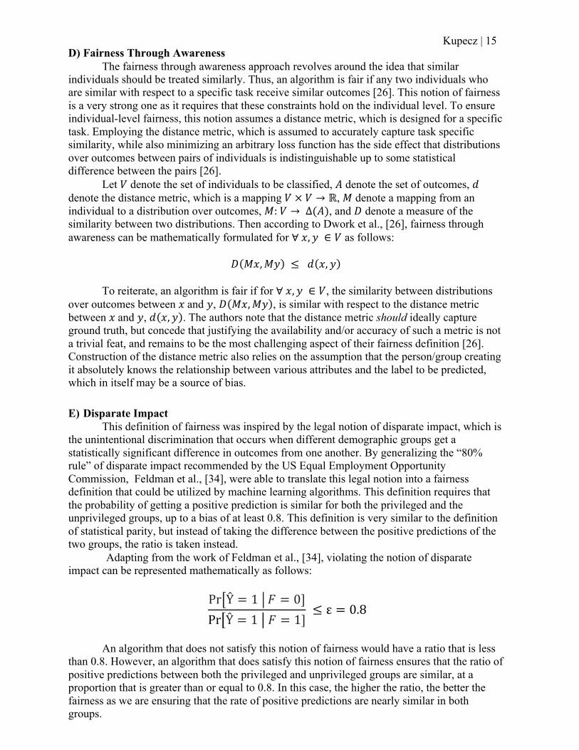
E) Disparate Impact

This definition of fairness was inspired by the legal notion of disparate impact, which is the unintentional discrimination that occurs when different demographic groups get a statistically significant difference in outcomes from one another. By generalizing the “80% rule” of disparate impact recommended by the US Equal Employment Opportunity Commission, Feldman et al., [34], were able to translate this legal notion into a fairness definition that could be utilized by machine learning algorithms. This definition requires that the probability of getting a positive prediction is similar for both the privileged and the unprivileged groups, up to a bias of at least 0.8. This definition is very similar to the definition of statistical parity, but instead of taking the difference between the positive predictions of the two groups, the ratio is taken instead.

Adapting from the work of Feldman et al., [34], violating the notion of disparate impact can be represented mathematically as follows:

Pr%Ŷ = 1! 𝐹 = 0]Pr%Ŷ = 1!𝐹 = 1]

≤ ε = 0.8

An algorithm that does not satisfy this notion of fairness would have a ratio that is less

than 0.8. However, an algorithm that does satisfy this notion of fairness ensures that the ratio of positive predictions between both the privileged and unprivileged groups are similar, at a proportion that is greater than or equal to 0.8. In this case, the higher the ratio, the better the fairness as we are ensuring that the rate of positive predictions are nearly similar in both groups.

16 | Kupecz

3.2 Comparing Fairness Definitions

There are clearly many different interpretations of what it means to be fair, and each definition aims to solve the same problem; namely the problem of creating more fair outputs of a model. With all of the variations in the definitions of fairness, those who aim to enhance fairness of their models face a huge dilemma in determining which definition to employ. One might think that if you want a really strict constraint on fairness, you should just frame the problem as a constrained optimization problem, with the constraint that multiple definitions of fairness are satisfied simultaneously. However, it has been shown that, except in highly specialized cases, many fairness definitions are often incompatible with one another, preventing one from satisfying multiple definitions of fairness simultaneously [35], [36]. Thus, those who aim to enhance fairness in their models must choose a fairness definition over the others. This choice ultimately requires critical thought on the application the definition will be employed in, as well as the appropriate societal, ethical, and legal context of the problem; there is no one-size-fits-all definition when it comes to fairness [37]. However, we can establish pros and cons of these various definitions at a high level.

A) Group Vs. Individual Notions

Group notions of fairness tend to be the most pervasive in the literature as they are simple, intuitive, do not require any assumptions about the data, and can easily be verified and implemented. However, group notions of fairness give guarantees to the average members of a group; they do not provide meaningful guarantees of fairness at the individual level [25]. For example, a definition may result in fair outputs with respect to the population of Black people as a whole, but this fairness won’t necessarily extend to subgroups of the Black population, such as those who are Black, queer, and disabled. In addition, group definitions of fairness require access to the protected attribute to ensure the fairness constraint, but in some applications, such as consumer lending, taking into account protected attributes such as race is illegal. Furthermore, certain group definitions of fairness, such as equalized odds and predictive parity, require access to the ground truth label [29], [32]. It may be the case that the “ground truth” was obtained in an unfair manner, such as through inherent historical bias that is present in the data.

As compared to group notions of fairness, individual notions of fairness are not as prevalent in the algorithmic fairness literature. They do, however, have stronger guarantees of fair outcomes on the individual level as compared to group notions. Dwork et al. achieve this by constraining the fairness metric between pairs of individuals [26]. This is seemingly the best type of fairness metric we can have as it treats similar individuals similarly, rather than treating groups similarly, which as stated above does not necessarily guarantee fairness with respect to subgroups. However, these types of definitions have an Achilles heel: they make strong assumptions about the process. For example, Dwork et al.’s fairness definition relies on the existence of a distance metric, and this metric is assumed to accurately compute the similarity between pairs of individuals. Construction of such a metric is by no means a trivial feat, as the authors even concede that this is the most challenging aspect of their work [26]. Construction of such a metric would require expert knowledge, and even with expert input, bias can creep up into its formulation. Furthermore the distance metric is task specific, meaning that a new distance metric would need to be formulated each time this definition is applied to different applications.

B) Clarifying Examples

It is important to reiterate that the definition of fairness one chooses to employ should depend on the application it is applied to, taking into account societal, ethical, and legal considerations. Let’s use criminal recidivism as an example. If one were to employ a metric such as statistical parity on a criminal recidivism model, one would be equalizing the number

Kupecz | 17

of positive predictions between both the privileged and unprivileged groups. From a societal standpoint, this definition would benefit society as we are making a strict constraint on identifying those who will recidivate, regardless of whether they truly will or were just predicted to, thus preventing them from potentially committing future crimes. However, from the criminals’ standpoint, this can be deemed unethical as we are not controlling for the rate of false positives, which is where a criminal was predicted to recidivate despite not actually recidivating. From the criminals’ standpoint, it might be more fair to employ a metric such as equalized odds, which equalizes the true positive rate and false positive rate between privileged and unprivileged groups. But from a societal standpoint, this definition may not necessarily suffice either since we are not controlling for the false negative rates, which is where a criminal was predicted to not recidivate despite actually recidivating. In those cases, we are letting some criminals out into society, which can be deemed as a harm to society. Choosing a specific fairness definition requires some tradeoffs, not only of accuracy and fairness, but also for the stakeholders involved in the process. These tradeoffs need to be discussed thoroughly and critically throughout the process, not only by computer scientists, but by all stakeholders involved [38].

As another example of the tradeoffs inherent in choosing a fairness definition, we can consider a model that predicts whether one should be accepted into an Ivy League university. Naturally one might think to use an individual notion of fairness, such as fairness through awareness, as these types of definitions aim to predict similar outcomes for similar people. However, employing this type of definition could be interpreted as a harm to the minority population, as they are not similar to the majority of applicants that get accepted into these types of universities; they often do not attend top-tier high schools, have access to similar opportunities, and do not have similar standardized testing scores [39]. Thus a definition that aims to treat similar people similarly would disadvantage those applicants who come from unprivileged backgrounds. Instead it might make more sense to employ a definition such as statistical parity, which would equalize the positive predictions between privileged and unprivileged groups. In this way, we are granting the unprivileged group the same chances of getting accepted, despite the fact that minority population is not similar to the majority population. Statistical parity may have also been helpful in the case of Amazon’s biased hiring algorithm. Since the bias in this case stemmed from lack of representation in their historical training data, by utilizing statistical parity we would be equalizing the positive predictions between the male and female groups, thus eliminating their issue of primarily hiring men.

Table 1: Brief Summary of Fairness Definitions

Definition Group vs. Individual

Metric Con

Statistical Parity

Group Equalizes Positive Predictions

Can be unfair if base rates between groups are different [1]

Predictive Parity

Group Equalizes Positive Predictive Value

Ground truth label may be biased

Equalized Odds

Group Equalizes TPR and FPR

Ground truth label may be biased

18 | Kupecz

Fairness Through Awareness

Individual Utilizes a distance metric to compute similarity between individuals

Construction of distance metric is non-trivial

Disparate Impact

Group Equalize ratio of positive predictions

Can be unfair if base rates between groups are different [1]

Kupecz | 19

4. Proposed Solutions The literature on fairness enhancing algorithms typically group the mechanisms into

three distinct groups: pre-process, in-process, and post-process. The group in which a solution is placed depends on where the mechanism is applied to in the model’s pipeline. Pre-process algorithms aim to make the biased training data more fair, before they are fed into a model. In-process algorithms incorporate fairness constraints during the process of learning. And post-process algorithms apply the fairness definitions to a model’s biased output, aiming to make the output more fair. This section will briefly cover a representative fairness enhancing mechanism for each category and will later compare the pros and cons of each group of mechanisms.

4.1 Pre-Process

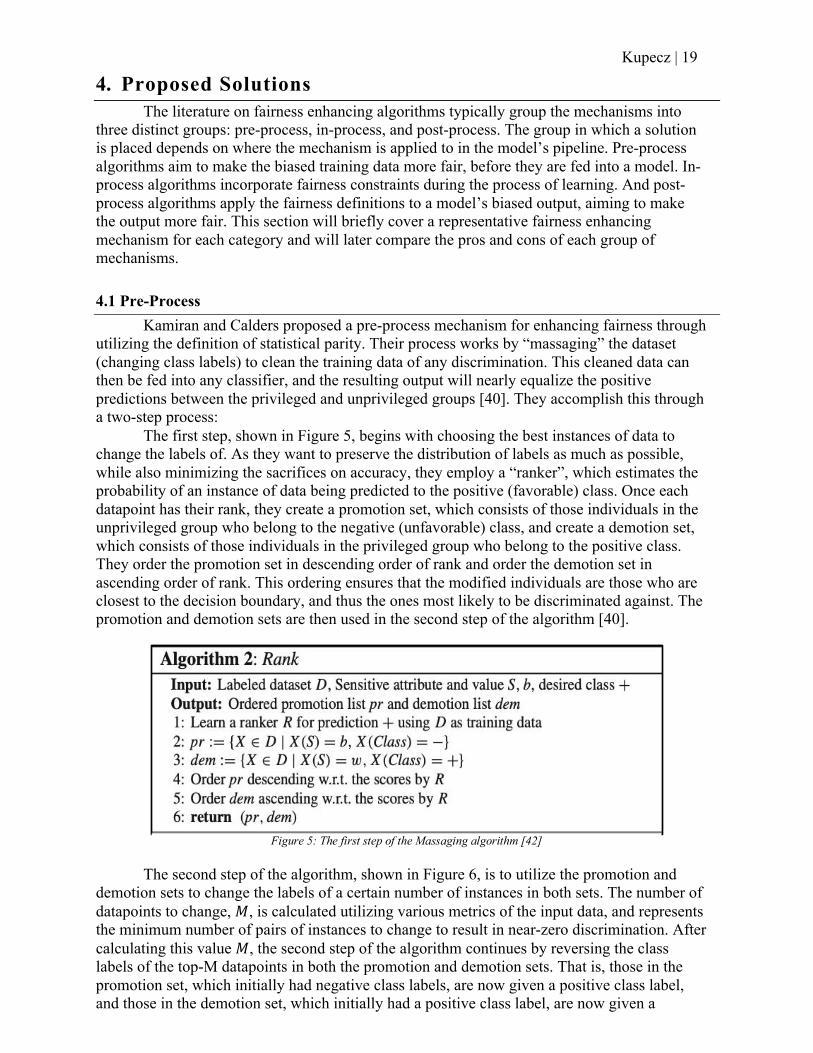
Kamiran and Calders proposed a pre-process mechanism for enhancing fairness through utilizing the definition of statistical parity. Their process works by “massaging” the dataset (changing class labels) to clean the training data of any discrimination. This cleaned data can then be fed into any classifier, and the resulting output will nearly equalize the positive predictions between the privileged and unprivileged groups [40]. They accomplish this through a two-step process:

The first step, shown in Figure 5, begins with choosing the best instances of data to change the labels of. As they want to preserve the distribution of labels as much as possible, while also minimizing the sacrifices on accuracy, they employ a “ranker”, which estimates the probability of an instance of data being predicted to the positive (favorable) class. Once each datapoint has their rank, they create a promotion set, which consists of those individuals in the unprivileged group who belong to the negative (unfavorable) class, and create a demotion set, which consists of those individuals in the privileged group who belong to the positive class. They order the promotion set in descending order of rank and order the demotion set in ascending order of rank. This ordering ensures that the modified individuals are those who are closest to the decision boundary, and thus the ones most likely to be discriminated against. The promotion and demotion sets are then used in the second step of the algorithm [40].

The second step of the algorithm, shown in Figure 6, is to utilize the promotion and demotion sets to change the labels of a certain number of instances in both sets. The number of datapoints to change, 𝑀, is calculated utilizing various metrics of the input data, and represents the minimum number of pairs of instances to change to result in near-zero discrimination. After calculating this value 𝑀, the second step of the algorithm continues by reversing the class labels of the top-M datapoints in both the promotion and demotion sets. That is, those in the promotion set, which initially had negative class labels, are now given a positive class label, and those in the demotion set, which initially had a positive class label, are now given a

Figure 5: The first step of the Massaging algorithm [42]

20 | Kupecz

negative class label. At the end of this algorithm, the dataset is now cleaned and ready to be fed into a model for learning [40].

One of the main benefits of this algorithm is that it is a pre-process mechanism, so a model need not be trained all over again, which could be costly, to incorporate fairness constraints. In addition, the instances of data that are changed are close to the decision boundary, which correspond to those individuals who are most likely to be discriminated against, and since we change an equal number of instances from the privileged and unprivileged groups, we are maintaining the same distribution of class labels that the uncleaned dataset had. However, one downside to this method is that it lacks explainability for why the data was discriminatory in the first place [1]. In addition, this mechanism can only be applied to situations in which there is only one binary protected attribute [42].

4.2 In-Process Agarwal et al. proposed an in-process mechanism for enhancing fairness by utilizing

randomized classifiers pulled from a distribution over a model space, and this approach allows many definitions of fairness to be applied to it. In the paper they primarily focus on statistical parity and equalized odds, but they note that many other definitions, excluding predictive parity, can be applied to this mechanism [41].

Given a classifier ℎ ∈ 𝐻, typical gradient descent tries to minimize the error on ℎ. This paper argues that by instead of just considering the model class H, one can get better fairness-accuracy tradeoffs by considering a randomized classifier 𝑄, and sampling a ℎ ∈ 𝐻 from 𝑄. Furthermore, this paper argues that by constraining the typical optimization problem above, we can get more fair outcomes. The constraint follows the form 𝑴𝝁(𝑄) ≤ 𝒄, where

• 𝑴 is a linear constraint matrix, 𝑴 ∈ ℝ|'|×|)|, where 𝐾 is the number of

constraints and 𝐽 is the number of features. • 𝑪 is a vector of acceptability for the 𝐾 linear constraints, set to 0 in most

examples. • 𝝁 is a vector of conditional moments, which measures the output of Q against a

fairness definition.

So the constrained optimization problem for gradient descent now becomes minimizing the error on Q subject to the constraint defined in the above inequality. The paper frames this problem as a saddle point problem and utilizes Lagrange multipliers for each of the K constraints to form the Lagrangian: 𝐿(𝑄, 𝝀) = 𝑒𝑟𝑟(𝑄) +𝝀$(𝑴𝝁(𝑄) − 𝒄). To find the saddle point, Agarwal et al. take a game-theoretic approach where the saddle point is the equilibrium

Figure 6: The second step of the Massaging algorithm [42]

Kupecz | 21

of the zero-sum game between two players. The first player, the Q-player, chooses a Q and the second player, the 𝜆-player, chooses a vector of Lagrange multipliers. The Lagrangian, 𝐿(𝑄, 𝝀), represents how much the Q-player has to pay the 𝜆-player after they make their choices. At the saddle point, neither player wants to deviate from their choices, so we have found the classifier that minimizes the error subject to the given constraints [45].

As one proceeds through the algorithm, shown above, the upper and lower bounds on the Lagrangian get closer together. Once the difference between the current best Lagrangian, calculated from the current best 𝑄 and the current best 𝝀, and the upper/lower bounds of the Lagrangian satisfy some accuracy threshold 𝜈, then the algorithm has converged on the 𝜈-approximate saddle point and we can return the classifier. Otherwise, we update the weights of the model, based on the fairness violations and learning rate, and continue through more iterations. The logic here is that we are using our best-guess functions, 𝑩𝑬𝑺𝑻* and 𝑩𝑬𝑺𝑻+, to incrementally and competitively update the values of 𝑄 and 𝝀. Once these best guesses of 𝑄 and 𝝀 converge to give us the near similar values for L(𝑄, 𝝀), then they have converged on a solution to the optimization problem.

Some of the main benefits of this approach are that many fairness definitions can be formulated as a set of linear constraints, and so can be applied to this game-theoretic approach, it allows for any classifier representations, it has provable guarantees, and the results of this method have performed significantly better as compared to baselines and other fairness approaches. This approach also optimizes the tradeoff between any single fairness definition constraint and accuracy [45]. In addition, the authors have noted that the algorithm typically requires 5 iterations before it returns a solution, so the time-complexity of this mechanism is reasonable [42]. However one negative to this approach is that if one wanted to employ this, one would have to retrain a whole classifier, which can be costly. In addition, the authors have noted that the algorithms time complexity scales quadratically in the number of training instances, which may be disadvantageous depending on the application. Furthermore, as noted earlier, the fairness definition of predictive parity cannot be used when using this mechanism, so applications in which predictive parity would be useful suffer from this disadvantage [46].

Figure 7: Reductions approach algorithm [45]

22 | Kupecz

4.3 Post-Process

Menon and Williamson created a post-process approach to enhancing the fairness of a model’s output by utilizing the definition of statistical parity. In essence, they aim to identify separate thresholds for the different groups, privileged and unprivileged, in a way that equalizes the frequency of positive predictions between groups. Their method accomplishes this through construction of a randomized classifier that maximizes accuracy while also minimizing the violation of statistical parity; that is they find the classifier with the optimal tradeoff between fairness and accuracy [5].

Their method consists of estimating 𝜂 and �̅�,", which are the class probabilities for samples of the joint distributions consisting of the pairs (𝑥- , 𝑦-) and pairs (𝑥- , 𝑦P-) respectively, where 𝑥- represents the features of instance 𝑖, 𝑦- represents the label given to instance 𝑖, and 𝑦P- represents the protected attribute value of instance 𝑖. They estimate these values through logistic regression. Once they have 𝜂 and �̅�,", they utilize these estimates to compute a thresholding score function, given by 𝑠, which computes the threshold for a particular instance of data (and thus a particular group). This function also depends on input parameters such as 𝜆, which is the fairness-accuracy tradeoff parameter, as well as 𝑐 and 𝑐̅, which are cost parameters. After they have this thresholding score function, they simply return a randomized classifier that maps an instance of data to a value determined by the output of a step function, whose input is the thresholding score of the particular instance of data being predicted [27]. The algorithm is presented below.

There are some favorable properties of this approach to fairness. First, like pre-processing approaches, one does not need to retrain their whole model to enhance fairness; one just needs to train a model on the output of the model being enhanced. In addition, the algorithm involves a convex optimization, so this allows it to be solved in polynomial time. Furthermore, once the estimates of 𝜂 and �̅�," have been calculated, one does not need to recalculate these values to tune their fairness constraints 𝜆 and 𝑐. One only needs to alter these fairness constraints, which will result in a different thresholding cutoff given by function 𝑠 [27]. However, the authors do concede that the result of the algorithm may be suboptimal, as there are bound to be imperfections in the estimation of class probabilities. This suboptimality is exacerbated in datasets in which there is a finite sample to be learned on, and it is

Figure 8: Post-processing Algorithm [27]

Kupecz | 23

exacerbated in certain classes of models where the true class probability may not be expressible [27].

4.4 Comparing Mechanism Types

In addition to there being multiple fairness definitions to choose from, we have also seen how there are multiple mechanism types one must choose from before they implement their chosen definition. Pre-process and post-process mechanisms are beneficial when one cannot retrain a whole model, whether that be due to time constraints or money constraints. In addition, these mechanisms are beneficial as they do not presuppose any model architecture; they are versatile in their application. Between all mechanism types, however, post-process mechanisms have been noted to obtain suboptimal results [43]. Pre-process mechanisms, however, harm the explainability of the results of a model since we modify the input data given to the model, which can be considered a black box algorithm [1]. Explainability of results may be an important factor to consider in use cases that affect the future of the individual a decision is being made about. In-process mechanisms are beneficial as they allow you to incorporate fairness constraints into the learning process itself and allow you to control the desired fairness-accuracy tradeoff [1]. This can allow for more complex associations to be formed, and they are also beneficial since you do not have to worry about modifying the input data or the output data. The main disadvantages of in-process mechanisms, however, are that you would be required to retrain your model, which can be time consuming and costly, and specific solutions are tailored to specific model architectures.

As with fairness definitions, the choice in which solution group to use depends on the situation it will be applied to. Critical thought about the context of the application as well as the feasibility of implementing the solution need to be taken into account before moving ahead with enhancing fairness. Although each proposed solution purports to be better than pre-existing solutions, the effectiveness of any one mechanism will ultimately depend on the application it is applied to.

24 | Kupecz

5. Novel Solutions

A) ModelChain ModelChain is an application of the Blockchain technology to create a decentralized,

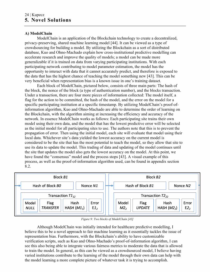
privacy-preserving, shared machine learning model [44]. It can be viewed as a type of crowdsourcing for building a model. By utilizing the Blockchain as a sort of distributed database, Kuo and Ohno-Machado explain how cross-institutional predictive modelling can accelerate research and improve the quality of models; a model can be made more generalizable if it is trained on data from varying participating institutions. With each participating network contributing to model parameter estimation, the model has the opportunity to interact with data that it cannot accurately predict, and therefore is exposed to the data that has the highest chance of teaching the model something new [43]. This can be very beneficial when representation bias is a known issue in one’s training dataset.

Each block of ModelChain, pictured below, consists of three main parts: The hash of the block, the nonce of the block (a type of authentication number), and the blocks transaction. Under a transaction, there are four more pieces of information collected: The model itself, a flag for the action to be committed, the hash of the model, and the error on the model for a specific participating institution at a specific timestamp. By utilizing ModelChain’s proof-of-information algorithm, Kuo and Ohno-Machado are able to determine the order of learning on the Blockchain, with the algorithm aiming at increasing the efficiency and accuracy of the network. In essence ModelChain works as follows: Each participating site trains their own model using their own data, and the model that has the lowest predictive error will be selected as the initial model for all participating sites to use. The authors note that this is to prevent the propagation of error. Then using the initial model, each site will evaluate that model using their local data. Whichever site’s data yielded the lowest accuracy on the current model is considered to be the site that has the most potential to teach the model, so they allow that site to use its data to update the model. This trading of data and updating of the model continues until the site that updates the model also gets the lowest accuracy on the model. At this point, we have found the “consensus” model and the process stops [43]. A visual example of this process, as well as the proof-of-information algorithm used, can be found in appendix section 8.2.

Although ModelChain was initially intended for healthcare predictive modelling, I believe this to be a novel approach to fair machine learning as it essentially tackles the issue of representation bias. Furthermore, with the Blockchain’s ability to have customizable verification scripts, such as Kuo and Ohno-Machado’s proof-of-information algorithm, I can see this also being able to integrate various fairness metrics to moderate the data that is allowed to train the model. In general, as this can be viewed as a crowdsourced model, I believe having varied institutions contribute to the learning of the model through their own data can help with the model learning a more complete picture of whatever task it is trying to accomplish.

Figure 9: Two blocks of ModelChain [43]

Kupecz | 25

B) AIF-360 Tool Research developers at IBM created the AI-Fairness 360 toolkit (AIF-360), which is the

first open-source toolkit focused on tackling issues relating to algorithmic fairness [45]. Although not an algorithmic solution to the problem itself, I found this to be a novel approach to tackle one of the issues in the field of algorithmic fairness; that of the situational nature for using various fairness definitions and fairness-enhancing mechanisms. The AIF-360 toolkit packages over 70 bias detection metrics, multiple bias mitigation algorithms, whether it be a pre-process, in-process, or post-process algorithms, and also includes metric explanations to facilitate the understanding of results [44]. This toolkit embodies the idea that various metrics and mechanisms should be used for different scenarios.

The authors note that the ultimate goal for the AIF-360 toolkit is to promote a deeper understanding of the various metrics and mechanisms of fairness related work, as it provides a common framework for fairness researchers to share and evaluate fairness-enhancing algorithms. In addition, the toolkit acts as a great transition for integrating these bias mitigation algorithms for use in industrial settings, and perhaps will become a staple such as the Sci-Kit package. Although the first of its kind, the AIF-360 toolkit encourages a common framework for working with algorithmic fairness and increases the transparency of results through their use of metric explanations. The toolkit also provides realistic tutorial examples and Jupyter notebooks to help those new to fairness quickly adapt and learn their tool [44]. As fairness research becomes more and more commonplace, a test-suite that gathers various metrics and algorithms in an easy to use library will be crucial for widespread adoption and understanding of the field.

C) FairGAN

Generative Adversarial Networks (GAN) have become increasingly popular for their ability to learn deep representations of data in the absence of extensively annotated training data, and have been applied throughout a plethora of areas [46]. In the general game theoretic approach, a generative model goes against a discriminative model, the adversary, with the aim that the competition between the two will drive both models to improve their methods [47]. So as the generative model gets better at generating data, the discriminative model must get better at discriminating the data, forcing the generative model to become even better at generating

Figure 10: FairGAN utilizes 1 generator and 2 discriminators.

26 | Kupecz

data. This cyclic game continues until an equilibrium is reached, at which point the generator has created high quality synthetic data [46].

Xu et al., [48], adapted the idea of GANs and applied it to the case of fair data generation. Ultimately they utilized GANs to create synthetic data that is free from disparate impact, but also retains data utility. Thus, by training a model on this synthetic data, the classifier will not be able to discriminate during the process of its decisions on the basis of disparate impact [47]. Their approach utilized one generative model and two discriminative models. The generative model’s goal is to generate synthetic samples of the input data, conditioned on the protected attribute. Then one of the discriminator’s goals is to identify whether this generated sample came from the real data set or not; the aim of the generator is to fool this discriminator into thinking it came from the real data set. The job of the second discriminator is to determine if the generated data belongs to the privileged or unprivileged group; the aim of the generator in this case is to fool this discriminator into thinking it came from a privileged group, as this group is not typically discriminated against. At the end of the game, the generative model has successfully produced high quality, synthetic data that retains much of the utility of the real input data [47].

Their work demonstrated promising results with the effectiveness of FairGAN to produce synthetic data that is free of disparate impact as well as data that retains much of its utility [47]. Being as this is the first application of GANs to tackle the issue of fairness, this approach lacks robustness of other methods that allow many fairness definitions to be integrated into it. The authors note, however, that their future work plans to improve on FairGAN by allowing it to incorporate fairness definitions such as equalized odds and statistical parity.

Kupecz | 27

6. Conclusion & Discussion

As we have seen, there have been a plethora of fairness definitions that have been proposed within the couple of decades that the field of algorithmic fairness has been around for. One unifying fairness definition that can be applied to any scenario has yet to be found, if it even exists. Therefore it remains crucial to critically think of and thoroughly understand the situation that calls for fairness, and to choose the most appropriate definition for that case; the choice is situational. In addition, once a fairness definition has been chosen, one will need to choose the most appropriate solution on a situational basis as well; it may be too costly to retrain a whole model, or perhaps it’s not feasible to constantly run pre-process and post-process algorithms to yield fair outputs. Despite the focus on fair classification in this paper, a lot of the information presented here extends to other types of AI applications, such as clustering, natural language processing, and computer vision, although each field presents their own additional challenges.

In addition to the focus that needs to be placed on grouping fairness definitions and solutions to their most applicable domains, the field of algorithmic fairness also needs to take into account the idea of intersectionality, or the idea that individuals belong to multiple groups. As discussed previously, group definitions may result in fair outcomes for the group as a whole, but this does not necessarily extend to subgroups. More research must be done on finding ways to ensure fairness with respect to sensitive subgroups. Furthermore, algorithmic fairness has primarily focused on binary sensitive attributes, for example marking minority groups as unprivileged and all others are privileged, but even between minority groups there can be issues of bias and unfairness. This is definitely the case when considering people with disabilities. For that reason, it may be of interest to investigate solutions which can handle multiple sensitive attribute values.

28 | Kupecz

7. Works Referenced [1] D. Pessach and E. Shmueli, “Algorithmic fairness,” arXiv, 2020, doi: 10.1257/pandp.20181018. [2] C. O’Neil, Weapons of Math Destruction, 1st ed. Crown, 2016. [3] B. Zhang and A. Dafoe, Artificial Intelligence: American Attitudes and Trends, no. January. 2019. [4] R. Benjamin, Race After Technology: Abolitionist Tools for the New Jim Code, 1st ed. Polity Press, 2019. [5] A. K. Menon and R. C. Williamson, “The cost of fairness in classification,” arXiv, pp. 1–12, 2017. [6] R. Bartlett et al., “Consumer-Lending Discrimination in the FinTech Era,” pp. 1–51, 2019, [Online]. Available:

http://www.nber.org/papers/w25943. [7] M. Weber, S. Botros, M. Yurochkin, and V. Markov, “Black loans matter: Distributionally robust fairness for fighting

subgroup discrimination,” arXiv, 2020. [8] J. Dastin, “Amazon scraps secret AI recruiting tool that showed bias against women,” Reuters, 2018. [9] L. K. Julia Angwin, Jeff Larson, Surya Mattu, “Machine Bias,” ProPublica, May 23, 2016. [10] Northpointe, “Practitioner’s Guide to COMPAS Core,” pp. 1–62, 2015. [11] L. K. Julia Angwin, Jeff Larson, Surya Mattu, “How We Analyzed the COMPAS Recidivism Algorithm,” ProPublica, May

23, 2016. [12] W. Dieterich, C. Mendoza, and T. Brennan, “COMPAS Risk Scales: Demonstrating Accuracy Equity and Predictive Parity,”

Perform. COMPAS Risk Scales Broward Cty., pp. 1–37, 2016. [13] “Google apologises for Photos app’s racist blunder,” BBC, Jul. 01, 2015. [14] M. Teodorescu, “Protected Attributes and ‘Fairness through Unawareness,’” MIT OCW, 2019.

https://ocw.mit.edu/resources/res-ec-001-exploring-fairness-in-machine-learning-for-international-development-spring-2020/module-three-framework/protected-attributes/ (accessed Dec. 04, 2021).

[15] S. Elbassuoni, S. Amer-Yahia, and A. Ghizzawi, “Fairness of Scoring in Online Job Marketplaces,” ACM/IMS Trans. Data Sci., vol. 1, no. 4, pp. 1–30, 2020, doi: 10.1145/3402883.

[16] S. Yeom, A. Datta, and M. Fredrikson, “Hunting for discriminatory proxies in linear regression models,” Adv. Neural Inf. Process. Syst., vol. 2018-Decem, no. NeurIPS, pp. 4568–4578, 2018.

[17] G. Yona, “A Gentle Introduction to the Discussion on Algorithmic Fairness,” towardsdatascience, 2017. https://towardsdatascience.com/a-gentle-introduction-to-the-discussion-on-algorithmic-fairness-740bbb469b6.

[18] T. Mahoney, K. R. Varshney, and M. Hind, AI Fairness. . [19] M. Mansoury, H. Abdollahpouri, M. Pechenizkiy, B. Mobasher, and R. Burke, “Feedback Loop and Bias Amplification in

Recommender Systems,” Int. Conf. Inf. Knowl. Manag. Proc., pp. 2145–2148, 2020, doi: 10.1145/3340531.3412152. [20] “Confusion matrix - Wikipedia,” En.wikipedia.org, 2021. https://en.wikipedia.org/wiki/Confusion_matrix. [21] T. Hellström, V. Dignum, and S. Bensch, “Bias in machine learning - what is it good for?,” CEUR Workshop Proc., vol. 2659,

pp. 3–10, 2020. [22] F. Martínez-Plumed, C. Ferri, D. Nieves, and J. Hernández-Orallo, “Fairness and missing values,” arXiv, 2019. [23] H. Suresh and J. V. Guttag, “A framework for understanding unintended consequences of machine learning,” arXiv, 2019. [24] J. Buolamwini and T. Gebru, “Gender Shades: Intersectional Accuracy Disparities in Commercial Gender Classification,”

Proc. Mach. Learn. Res., vol. 81, 2018, [Online]. Available: http://proceedings.mlr.press/v81/buolamwini18a/buolamwini18a.pdf.

[25] A. Chouldechova and A. Roth, “The frontiers of fairness in machine learning,” arXiv, pp. 1–13, 2018. [26] C. Dwork, M. Hardt, T. Pitassi, O. Reingold, and R. Zemel, “Fairness through awareness,” ITCS 2012 - Innov. Theor.

Comput. Sci. Conf., pp. 214–226, 2012, doi: 10.1145/2090236.2090255. [27] S. Verma and J. Rubin, “Fairness definitions explained,” Proc. - Int. Conf. Softw. Eng., pp. 1–7, 2018, doi:

10.1145/3194770.3194776. [28] F. J. W. M. Dankers, A. Traverso, L. Wee, and S. M. J. van Kuijk, “Prediction Modeling Methodology,” in Fundamentals of

Clinical Data Science, P. Kubben, M. Dumontier, and A. Dekker, Eds. Cham: Springer International Publishing, 2019, pp. 101–120.

[29] A. Chouldechova, “Fair Prediction with Disparate Impact: A Study of Bias in Recidivism Prediction Instruments,” Big Data, vol. 5, no. 2, pp. 153–163, 2017, doi: 10.1089/big.2016.0047.

[30] H. Wang and H. Zheng, “False Positive Rate,” in Encyclopedia of Systems Biology, W. Dubitzky, O. Wolkenhauer, K.-H. Cho, and H. Yokota, Eds. New York, NY: Springer New York, 2013, p. 732.

[31] H. Wang and H. Zheng, “True Positive Rate,” in Encyclopedia of Systems Biology, W. Dubitzky, O. Wolkenhauer, K.-H. Cho, and H. Yokota, Eds. New York, NY: Springer New York, 2013, pp. 2302–2303.

[32] M. Hardt, E. Price, and N. Srebro, “Equality of opportunity in supervised learning,” Adv. Neural Inf. Process. Syst., pp. 3323–3331, 2016.

[33] N. Mehrabi, F. Morstatter, N. Saxena, K. Lerman, and A. Galstyan, “A survey on bias and fairness in machine learning,” arXiv, 2019.

[34] M. Feldman, S. A. Friedler, J. Moeller, C. Scheidegger, and S. Venkatasubramanian, “Certifying and removing disparate impact,” Proc. ACM SIGKDD Int. Conf. Knowl. Discov. Data Min., vol. 2015-Augus, pp. 259–268, 2015, doi: 10.1145/2783258.2783311.

[35] J. Kleinberg, S. Mullainathan, and M. Raghavan, “Inherent trade-offs in the fair determination of risk scores,” Leibniz Int. Proc. Informatics, LIPIcs, vol. 67, pp. 1–23, 2017, doi: 10.4230/LIPIcs.ITCS.2017.43.

[36] S. A. Friedler, C. Scheidegger, and S. Venkatasubramanian, “On the (im)possibility of fairness,” no. im, pp. 1–16, 2016,

Kupecz | 29

[Online]. Available: http://arxiv.org/abs/1609.07236. [37] doaa Abu Elyounes, “Contextual Fairness: A Legal and Policy Analysis of Algorithmic Fairness,” SSRN Electron. J., pp. 1–

67, 2019, doi: 10.2139/ssrn.3478296. [38] R. Berk, H. Heidari, S. Jabbari, M. Kearns, and A. Roth, “Fairness in Criminal Justice Risk Assessments: The State of the

Art,” Sociol. Methods Res., vol. 50, no. 1, pp. 3–44, 2021, doi: 10.1177/0049124118782533. [39] College Board, “2018 Total group SAT suite of assessments annual report,” p. 16, 2018. [40] F. Kamiran and T. Calders, Data preprocessing techniques for classification without discrimination, vol. 33, no. 1. 2012. [41] A. Agarwal, A. Beygelzimer, M. Dudík, J. Langford, and H. Wallach, “A reductions approach to fair classification,” arXiv,

2018. [42] Miroslav Dudík, A Reductions Approach to Fair Classification. Vimeo, 2019. [43] B. Woodworth, “Learning Non-Discriminatory Predictors,” vol. 65, no. 2012, pp. 1–34, 2017. [44] T.-T. Kuo and L. Ohno-Machado, “ModelChain: Decentralized Privacy-Preserving Healthcare Predictive Modeling

Framework on Private Blockchain Networks,” CoRR, vol. abs/1802.0, 2018, [Online]. Available: http://arxiv.org/abs/1802.01746.

[45] R. K. E. Bellamy et al., “Ai fairness 360: An extensible toolkit for detecting, understanding, and mitigating unwanted algorithmic bias,” arXiv, 2018.

[46] A. Creswell, T. White, V. Dumoulin, K. Arulkumaran, B. Sengupta, and A. A. Bharath, “Generative Adversarial Networks: An Overview,” IEEE Signal Process. Mag., vol. 35, no. 1, pp. 53–65, 2018, doi: 10.1109/MSP.2017.2765202.

[47] I. Goodfellow et al., “Generative adversarial networks,” Commun. ACM, vol. 63, no. 11, pp. 139–144, 2020, doi: 10.1145/3422622.

[48] D. Xu, S. Yuan, L. Zhang, and X. Wu, “FairGAN: Fairness-aware Generative Adversarial Networks,” Proc. - 2018 IEEE Int. Conf. Big Data, Big Data 2018, pp. 570–575, 2019, doi: 10.1109/BigData.2018.8622525.

30 | Kupecz

8. Appendix

8.1 Aggregation Bias + Representation Bias Below are scatterplots of the hypothetical situation described in section 2.3(d) where an

unfair linear regression model was tasked with predicting if one will repay a loan. The circles represent the majority group in the population whereas the squares represent the minority group in the population. Coloring a shape green means that the person successfully repaid a loan, whereas red means that they did not repay a loan. Overall we can see that the minority group tends to have a lower income and a lower GPA and the majority group tends to have a higher income and higher GPA. Despite this, the minority population successfully repaid loans 70% of the time, whereas the majority population successfully repaid loans about 45% of the time.

We can see that applying a single model to the aggregated data results in the minority

population being predicted as not able to repay a loan, despite the fact that the minority population has a higher rate of repayment as compared to the majority population.

$100

k$1

0kIncome

GPA0.0 4.0

$100

kIncome

$10k

GPA0.0 4.0

c) Scatterplot for the majority group only. c) Scatterplot for the minority group only.

$100

k$1

0kIncome

GPA0.0 4.0

c) Scatterplot for the combined data.

Kupecz | 31

8.2 ModelChain

A) Proof-of-information Algorithm

B) Example of Execution

A few iterations of the ModelChain learning process [43]

ModelChain's proof-of-information algorithm [43]