© 2011 ANSYS, Inc. June 21, 2012 1

ANSYS Workbench for Process Compression and Scalability

Jiaping Zhang, Technical Service Engineer,

Ansys Inc. Houston Office

Jiaping.Zhang@Ansys.com

© 2011 ANSYS, Inc. June 21, 2012 2

Agenda

1. Ansys Workbench & Mechanical: An Introduction

2. 6 Steps to a Successful FEA Simulation

3. Physics Coupling and External Data Import

4. ACT Preview: Customizing the User Interface

© 2011 ANSYS, Inc. June 21, 2012 3

Agenda

1. Ansys Workbench & Mechanical: An Introduction

2. 6 Steps to a Successful FEA Simulation

3. Physics Coupling and External Data Import

4. ACT Preview: Customizing the User Interface

© 2011 ANSYS, Inc. June 21, 2012 4

Setup Solving Results Variations

One simulation

Setup Solving Results Variations

N simulations

Shorten setup time for a single simulation Reduce solving time Simplify results analysis Increase simulations in fixed time

Productivity Challenge

Boost Productivity HPC+GPU

© 2011 ANSYS, Inc. June 21, 2012 5

Workbench: Shorten Setup Time

Multiphysics Workflow

Automatic Contact

Automatic Meshing CAD& Parametric

© 2011 ANSYS, Inc. June 21, 2012 6

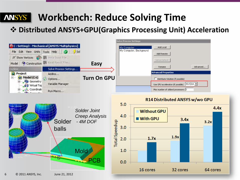
Workbench: Reduce Solving Time Distributed ANSYS+GPU(Graphics Processing Unit) Acceleration

Mold PCB

Solder balls

Solder Joint

Creep Analysis

- 4M DOF

Easy Turn On GPU

© 2011 ANSYS, Inc. June 21, 2012 7

Workbench: Simplify Postprocessing

© 2011 ANSYS, Inc. June 21, 2012 8

Workbench: Allows Variations

Response Surface Single Parameter

Sensitivity Study Goal Driven Optimization

© 2011 ANSYS, Inc. June 21, 2012 9

Agenda

1. Ansys Workbench & Mechanical: An Introduction

2. 6 Steps to a Successful FEA Simulation

3. Physics Coupling and External Data Import

4. ACT Preview: Customizing the User Interface

© 2011 ANSYS, Inc. June 21, 2012 10

Step 1: Define the Simulation Workflow

© 2011 ANSYS, Inc. June 21, 2012 11

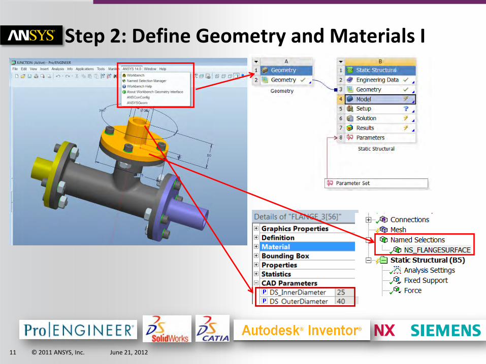
Step 2: Define Geometry and Materials I

© 2011 ANSYS, Inc. June 21, 2012 12

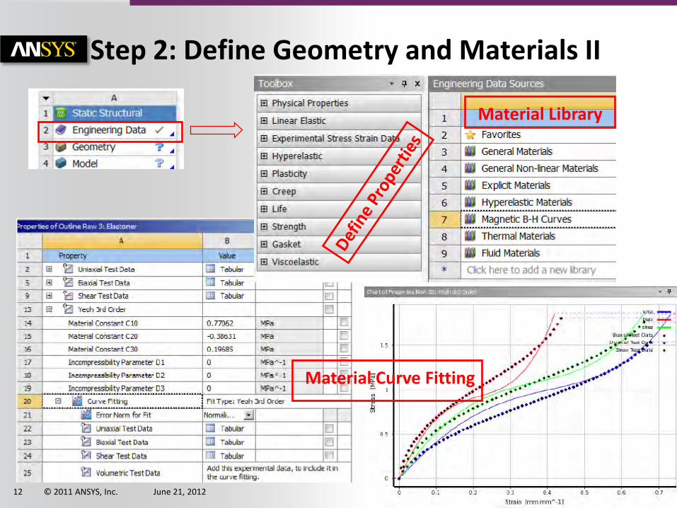
Step 2: Define Geometry and Materials II

Material Library

Material Curve Fitting

© 2011 ANSYS, Inc. June 21, 2012 13

Step 3: Define Connections between Bodies

© 2011 ANSYS, Inc. June 21, 2012 14

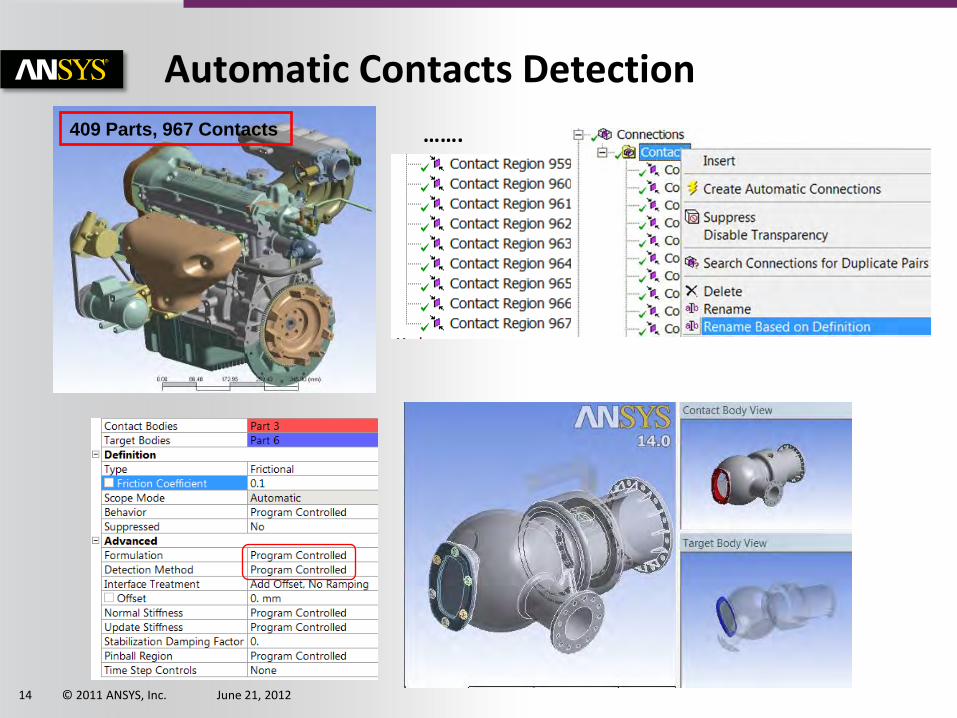
Automatic Contacts Detection

409 Parts, 967 Contacts …….

© 2011 ANSYS, Inc. June 21, 2012 15

More Connections are Available

Joint

Beam

Spring

Mesh connection

Spot Welds

© 2011 ANSYS, Inc. June 21, 2012 16

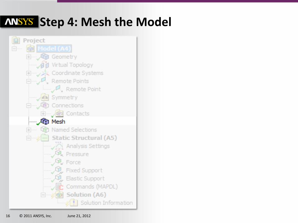
Step 4: Mesh the Model

© 2011 ANSYS, Inc. June 21, 2012 17

Global Mesh Control

Curvature “On”

Proximity “On”

© 2011 ANSYS, Inc. June 21, 2012 18

More Local Controls are Available

© 2011 ANSYS, Inc. June 21, 2012 19

Adaptive Mesh Refinement for Convergence

© 2011 ANSYS, Inc. June 21, 2012 20

Step 5: Define Loads and Boundary Conditions

© 2011 ANSYS, Inc. June 21, 2012 21

Loads and Boundary Condition Options

© 2011 ANSYS, Inc. June 21, 2012 22

Applying Loads to Nodes

“Nodal orientation” allows users to assign a coordinate system to node or nodal sets

Direct FE loads and boundary conditions can be applied to selected nodes, whose direction is defined by “Nodal orientation”

Nodes are oriented in cylindrical system for loads and boundary condition definitions

© 2011 ANSYS, Inc. June 21, 2012 23

Step 6: Understanding and Verifying Results

© 2011 ANSYS, Inc. June 21, 2012 24

Thoroughly Investigate Your Results

© 2011 ANSYS, Inc. June 21, 2012 25

Check The Quality of Your Results

Applied Load

Reactive Force

© 2011 ANSYS, Inc. June 21, 2012 26

Create a Project Report

© 2011 ANSYS, Inc. June 21, 2012 27

Enhance Simulation Using Command Objects

© 2011 ANSYS, Inc. June 21, 2012 28

Command Object Example: Contact Setting

Frictional Surface

Set shear stress limit

© 2011 ANSYS, Inc. June 21, 2012 29

Apply Constraint and Loading on this surface

Load step 2: Clamp top surface

Load Step 3: Apply vertical loading to clamped surface

Command Object Example: Loading

© 2011 ANSYS, Inc. June 21, 2012 30

Command Object Example: PostProcessing

© 2011 ANSYS, Inc. June 21, 2012 31

Agenda

1. Ansys Workbench & Mechanical: An Introduction

2. 6 Steps to a Successful FEA Simulation

3. Physics Coupling and External Data Import

4. ACT Preview: Customizing the User Interface

© 2011 ANSYS, Inc. June 21, 2012 32

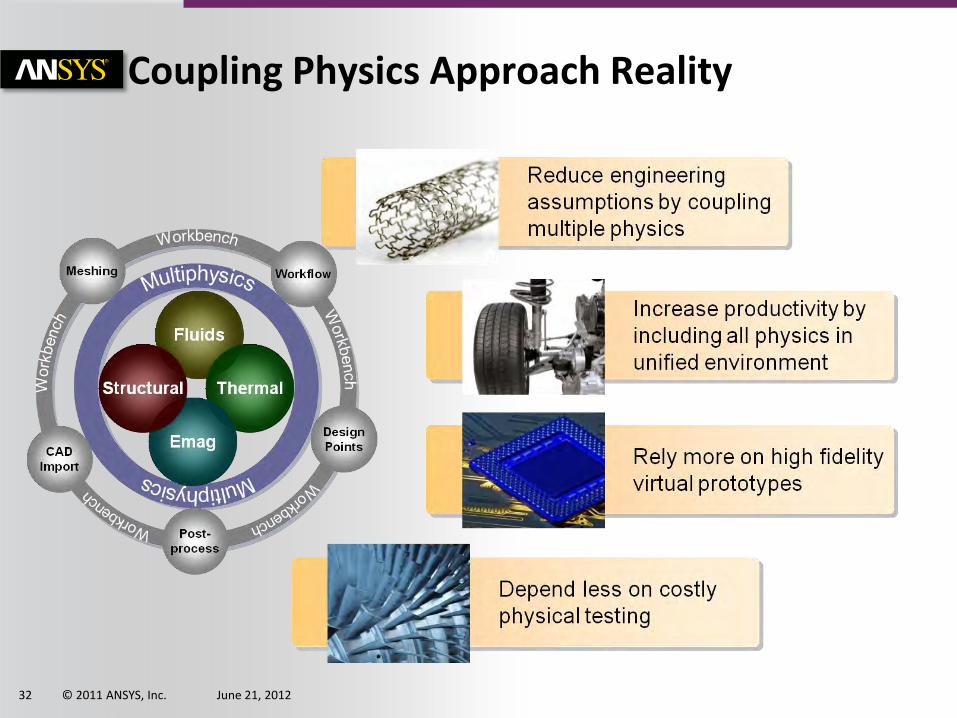
Coupling Physics Approach Reality

© 2011 ANSYS, Inc. June 21, 2012 33

ANSYS Solution for Multiphysics

Electromagnetic Simulation

Low Frequency

Maxwell

Simplorer

High Frequency

HFSS

SIwave

Mechanical Simulation

Implicit

ANSYS Mechanical

Explicit

ANSYS Explicit

ANSYS AUTODYN

ANSYS LS-DYNA

Computational Fluid Dynamics (CFD)

Electronics cooling

ANSYS Icepak

General CFD

ANSYS CFD

Structural Mechanics Fluid Dynamics

Electromagnetics

© 2011 ANSYS, Inc. June 21, 2012 34

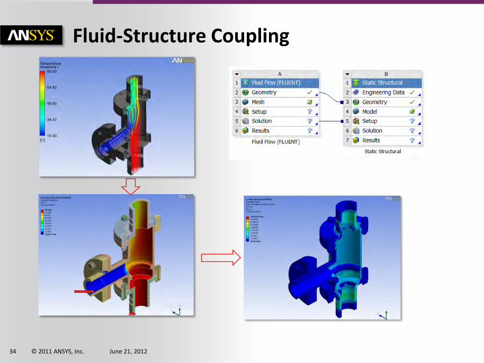
Fluid-Structure Coupling

© 2011 ANSYS, Inc. June 21, 2012 35

Electromagnetic-Structure Coupling

Magnetics forces will induce stresses(Example: Motor)

Resistive losses will cause thermal stress(Example: Satellite Dish Antenna)

© 2011 ANSYS, Inc. June 21, 2012 36

Electromagnetic-Fluid-Structure Coupling • Maxwell+Fluent

– One-way and two-way β coupling

• Combine with 1-way FSI

β

© 2011 ANSYS, Inc. June 21, 2012 37

External Data Mapping: Motivation

Exchange files are frequently encountered to transfer quantities from one simulation to another. Efficient mapping of point cloud data is required to account for misalignment, non matching units or scaling issues.

© 2011 ANSYS, Inc. June 21, 2012 38

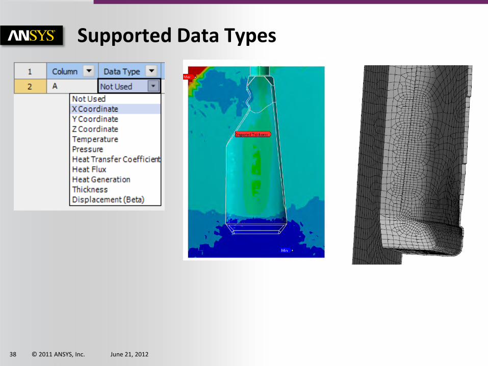
Supported Data Types

© 2011 ANSYS, Inc. June 21, 2012 39

Importing Multiple Files

Multiple files can be imported for transient analyses or to handle different data to be mapped on multiple bodies

© 2011 ANSYS, Inc. June 21, 2012 40

Validating the Mapped Data

Visual tools have been implemented to control how well the data has been mapped onto the target structure

Both the size of the spheres and their color provide indication of the mapping quality

© 2011 ANSYS, Inc. June 21, 2012 41

Agenda

1. Ansys Workbench & Mechanical: An Introduction

2. 6 Steps to a Successful FEA Simulation

3. Physics Coupling and External Data Import

4. ACT Preview: Customizing the User Interface

© 2011 ANSYS, Inc. June 21, 2012 42

Encapsulate APDL macros: Allows re-use of legacy APDL-scripts and encourages migration from MAPDL to Mechanical via “encapsulated macros”

MAPDL exposure: Fills the gap between MAPDL solver capabilities and their exposure in ANSYS Mechanical

New pre-processing features (custom loads and boundary conditions)

New post-processing features (custom results)

3rd party/in-house solver integration (Mechanical GUI)

ACT Introduction

Application Customization Toolkit (New in R14.0)

© 2011 ANSYS, Inc. June 21, 2012 43

Opportunity to migrate existing process automation from MAPDL to ANSYS Mechanical at “low cost”

Simple ACT Example

APDL

! APDL_script_for_convection.inp

! Input parameters:

esel,s,type,,10 cm,component,ELEM thickness = 0.005 film_coefficient = 200. temperature = 226.85 ! Treatment:

/prep7 et,100,152 keyop,100,8,2. et,1001,131 keyo,1001,3,2 sectype,1001,shell secdata,thickness,10 secoff,mid cmsel,s,component emodif,all,type,1001 emodif,all,secnum,1001 type,100 esurf fini alls /solu esel,s,type,,100 nsle sf,all,conv,film_coefficient,temperature alls

APDL ANSYS Mechanical

© 2011 ANSYS, Inc. June 21, 2012 44

ACT Structure

© 2011 ANSYS, Inc. June 21, 2012 45

Customize Toolbar Using XML

<load internalName="Convection on Blade" caption="Convection on Blade" icon="Convection" issupport="false" isload="true"> <version>1</version>

<callbacks> <onsolve>Convection_Blade_Computation</onsolve> </callbacks>

<details> <property internalName="Geometry" dataType="string" control="scoping"></property> <property internalName="Thickness" caption="Thickness" dataType="string" control="text"></property> <property internalName="Film Coefficient" caption="Film Coefficient" dataType="string" control="text"></property> <property internalName="Ambient Temperature" caption="Ambient Temperature" dataType="string" control="text"></property>

</details> </load>

XML definition:

© 2011 ANSYS, Inc. June 21, 2012 46

Define Internal Process Using Python

Python script:

# Get the scoped geometry:

propGeo = result.GetDPropertyFromName("Geometry") refIds = propGeo.Value

# Get the related mesh and create the component:

for refId in refIds: meshRegion = mesh.MeshRegion(refId) elementIds = meshRegion.Elements eid = aap.mesh.element[elementIds[0]].Id f.write("*get,ntyp,ELEM,"+eid.ToString()+",ATTR,TYPE\n") f.write("esel,s,type,,ntyp \n cm,component,ELEM")

# Get properties from the details view:

propThick = load.GetDPropertyFromName("Thickness") thickness = propThick.Value propCoef = load.GetDPropertyFromName("Film Coefficient") film_coefficient = propCoef.Value propTemp = load.GetDPropertyFromName("Ambient Temperature") temperature = propTemp.Value

# Insert the parameters for the APDL commands:

f.write("thickness="+thickness.ToString()+"\n") f.write("film_coefficient="+film_coefficient.ToString()+"\n") f.write("temperature="+temperature.ToString()+"\n") # Reuse the legacy APDL macros:

f.write("/input,APDL_script_for_convection.inp\n")

© 2011 ANSYS, Inc. June 21, 2012 47

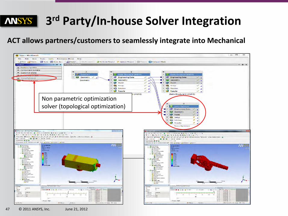
ACT allows partners/customers to seamlessly integrate into Mechanical

3rd Party/In-house Solver Integration

Non parametric optimization solver (topological optimization)

© 2011 ANSYS, Inc. June 21, 2012 48

Concluding Remarks

Compress setup process Simplify physics coupling and data import Allows User Customization

Workbench compresses and scale your simulation via:

© 2011 ANSYS, Inc. June 21, 2012 49

Thank you!