Fisheries biology, assessment and management

Welcome to the accompanying website for Fisheries biology, assessment and management by Michael King. This website contains answers to many of the practical exercises given at the end of each Chapter in the book.

The book

The new and completely revised 2007 edition of Fisheries biology, assessment and management includes an additional Chapter on marine ecology; this has been included due to the increasing need to manage ecosystems as well as fish stocks. Chapters on parameter estimation and stock assessment now include step­by­step instructions on building computer spreadsheet models, including simulations with random variations that realistically emulate the vagaries of nature. Sections on ecosystem management, co­management, community­based management and marine protected areas have been expanded to match the growing importance of these topics.

The author

Dr Michael King is a past Associate Director of the Faculty of Fisheries and Marine Environment at the Australian Maritime College. He has been team leader of international fisheries projects and is presently a fisheries consultant working in many countries from the Middle East to the South Pacific. He has extensive experience in fisheries training, the assessment, development and management of fisheries, and in promoting the community­based management of fisheries and the marine environment.

­­­­­­­­­­­­­­­­­­­­­­­­­­­­­­­­­­­­­­­­­­­­­­­­­­­­­­­­­­­­­­­­­­­­­­­­­­­­­­­­­­­­­­­

Chapter 1. Ecology and ecosystems

This Chapter is about the distribution, abundance and life­history of organisms and their place in ecosystems that vary from wetlands to the open seas. The Chapter also describes marine food chains, production from fisheries and the impacts of humans on marine ecosystems. The aim of the Chapter is to provide the reader with the broad ecological knowledge necessary for effective fisheries management.

As the exercises in Chapter 1 relate to local species and issues, specific answers cannot be provided here. However, some points for consideration are given below.

Exercise 1.1

Map the distribution and areas of either wetlands, salt marshes, mangroves, seagrass beds or coral reefs adjacent to your town or community. Consult records and interview older local inhabitants to discover if these areas are increasing or decreasing in size. What changes have occurred and why? Are the areas adequately protected at present.

When collecting oral history keep mind that some people may exaggerate. Some fishers, proud of their fishing skills, may overstate the size of catches. And although the views of older people are important links to the past, many tend to remember things as being better than they really were! Also, keep in mind that some marine and coastal areas may have been protected under traditional arrangements and community agreements rather than by modern laws and regulations (a browse of Chapter 6 may help in completing this Exercise).

Exercise 1.2

Obtain recent fish catch statistics for your country and review the status of the five most important species or fisheries. Consider the status of the resources (under­exploited, fully exploited, or over­ exploited) and whether rules and regulations applied to the fishery are effective.

First of all, consider what “important” means in the context of your country or local area. Importance can be defined in terms of either total catch weight, total catch value, the amount of local food produced, the amount of export income generated, or employment created. In some cases, the targeted species is of greater cultural significance than its value as food or an item to be traded; the flesh of turtles and giant clams, for example, are culturally important foods for many Pacific island peoples.

Exercise 1.3

Review the most serious threats to the coastal environment in an area with which you are familiar. What regulations apply to the area ­ and are these being enforced? What actions are being taken, or should be taken, to counteract these threats?

In some cases, local coastal environments are being affected by things that are happening some distance away from the area of concern. Silt pollution affecting a fishery in an estuary, for example, may have resulted from either farming or forestry operations many kilometres up river. It would be useful in an analysis to separate threats caused locally from those related to distant activities. The latter threats often cannot be addressed by a local community and usually require the integrated efforts of government agencies and community groups working together. Integrated Coastal Management (ICM), referred to in Chapter 6, takes into account the inter­dependence of ecosystems and the involvement of many different agencies (for example, those responsible for agriculture, forestry, fisheries, public works and water supply) and other stakeholders.

­­­­­­­­­­­­­­­­­­­­­­­­­­­­­­­­­­­­­­­­­­­­­­­­­­­­­­­­­­­­­­­­­­­­­­­­­­­­­­­­­­

Chapter 2. Exploited species

This Chapter is about exploited marine species, from bivalve molluscs on beaches to pelagic fish in the open sea. The aim of the Chapter is to familiarize the reader with the biology and life­cycles of species, including molluscs, crustaceans, echinoderms and fishes, which are targeted in fisheries around the world. Effective fisheries management depends on managers having at least some knowledge of the biology of the target species.

As the exercises in Chapter 2 relate to local species and issues, answers cannot be provided and some hints on collecting information are given.

Exercise 2.1

Prepare a resource status report on an exploited marine species that you are familiar with locally. The report should address the biology of the species, history of the fishery, status of the resource, current management measures and recommendations.

Staff of local fisheries management agencies are usually a good source of information. In addition, views on the management of the resource should be obtained from key stakeholders including the fishers, processors and those affected, sometimes adversely, by the fishery. Note that in some fisheries there are conflicts either between inshore and offshore fishers or between recreational and professional fishers targeting the same species.

Exercise 2.2

Conduct a brief survey of a local fish market. Make a list of all species offered for sale with estimate weights available, price per kg and place of origin. Interview sellers to find out where each species comes from and how the availability of the marketed species varies seasonally.

Keep in mind that not all market days will be the same ­ a greater variety or quantity of seafood may be available on particular days of the week. In some cultures, for example, preparations for Sunday feasts mean that Saturday is the most important day at the local fish market. In other cultures, religious beliefs result in Friday being the biggest fish marketing day of the week. A daily market survey should be carried out over a seven day period. Note that bad weather will reduce or prevent seafood reaching the market. An extension of this exercise would be to consider three or four key marketed species and conduct market surveys on their availability and price over a period of 12 months.

­­­­­­­­­­­­­­­­­­­­­­­­­­­­­­­­­­­­­­­­­­­­­­­­­­­­­­­­­­­­­­­­­­­­­

Chapter 3. Fishing and fishers

This Chapter is about fishers and their gear. A key aim of the chapter is for the reader to become familiar with the variety of fishing gear used, motivations for fishing and the environmental effects of fishing. Fishing gears from traps to purse seine nets are described. Reasons for fishing include recreation as well as the provision of food and income. All fishing operations have some environmental effects including those on targeted species, non­targeted species and marine ecosystems.

Exercise 3.1

Choose a particular type of fishing gear that is used locally and discuss how it is used, how selective it is, how much bycatch is caught in a typical operation, and how damaging it is to the environment.

Is the fishing gear used passively (like a gill net) or actively (like a towed trawl net)? What is its form and shape? ­ a drawing with typical dimensions would be useful. How is it used? ­ find out how long the gear is left in the water during a typical fishing operation and what species are caught. All fishing gear is environmentally damaging to some degree ­ find out how the particular gear chosen affects the marine environment and how this compares with other fishing gear. Here, the opinions of local fisheries agencies, fishers using the particular gear, fishers using different gear, and other users of the marine environment should be sought.

Exercise 3.2

An experiment involving covering the codend of a trawl net with a cover made of smaller mesh netting produced the following small sample. Make an initial estimate of the mean length at first capture, Lc.

The data given in the exercise can be arranged as shown in the table below (this is similar to Table 3.3 in the book). For each length class, the proportion retained is calculated as the number of fish in the codend divided by the total number caught. The right hand column contains values used in subsequent calculations.

­­­­­­­­­­­­­­­­­­­­­­­­­­­­­­­­­­­­­­­­­­­­­­­­­­­­­­­­­­­­­­­­­­­­­­­­­­­­­­­­­­­­­­­­­­­­­­­­­­­­­­­­­ length frequency frequency frequency proportion (cm) (codend) (cover) total retained (P) ln[(1­P)/P] ­­­­­­­­­­­­­­­­­­­­­­­­­­­­­­­­­­­­­­­­­­­­­­­­­­­­­­­­­­­­­­­­­­­­­­­­­­­­­­­­­­­­­­­­­­­­­­­­­­­­­­­­­ 9 0 8 8 0.00 (not defined) 10 1 9 10 0.10 2.20 12 3 11 14 0.21 1.30 14 3 13 16 0.19 1.47 16 12 8 20 0.60 ­0.41 18 14 4 18 0.78 ­1.25 20 13 2 15 0.87 ­1.87 22 25 1 26 0.96 ­3.22 ­­­­­­­­­­­­­­­­­­­­­­­­­­­­­­­­­­­­­­­­­­­­­­­­­­­­­­­­­­­­­­­­­­­­­­­­­­­­­­­­­­­­­­­­­­­­­­­­­­­­­­­­­

The data in the above table are now used to find the two constants in an S­shaped or logistic curve of the form:

P = 1/(1+exp[­r(L­ Lc)])

where r is a constant with a value which increases with the steepness of the selection curve, and Lc is the mean length at first capture. As described in the book, this equation may be transformed into:

ln[(1­P)/P] = rLc­ rL

which is of the form of a straight line where the slope, b = ­r and the intercept, a = rLc. The values of ln[(1­P)/P] in the above table may be plotted against L as shown in the Microsoft Excel spreadsheet below (which is similar to Figure 3.16b in the book) to provide an estimate of r and Lc as r = ­ (b), and, Lc = intercept/r.

The intercept is the y­axis intercept which, although off the scale of the graph, is given in the equation included on the graph as y = ­0.452x + 6.9762. From this, r = 0.452, and Lc = 6.976/0.452 = 15.4 cm.

y = ­0.452x + 6.9762 R 2 = 0.9609

­4.00

­3.00

­2.00

­1.00

0.00

1.00

2.00

3.00

5 10 15 20 25

length

ln[(1

­P)/P

]

The proportion retained may be plotted against length, and an S­shaped curve drawn through the points (as in Figure 3.16a in the book). The important point on the graph is the mean length at first capture (Lc), at which a fish has a 50% chance of being retained by the net (a 0.5 probability of being caught). The mean length at capture could also be estimated more directly by non­linear least squares using a computer­based search for the parameter values (Lc and r in this case) that result in a logistic curve fitting the observed data ­ see Exercise 3.3.

Exercise 3.3

Design a computer spreadsheet program that estimates the mean length at capture from the data in Table 3.3 using non­linear least squares as described in Appendix 4. See the example used to estimate mean length at maturity for the spreadsheet design.

Appendix 4.5 describes a spreadsheet program designed to estimate the mean length at sexual maturity. This spreadsheet can be adapted to estimate the mean length at capture as both are based on the s­shaped or logistic curve. In this case, trial values of r and Lc (say 0.5 and 15 respectively) are entered in the two cells at the top of column B of the spreadsheet shown below. Now length data and the observed proportion retained in the net are entered in columns A and B. Column C contains the proportion retained predicted by the logistic equation:

P = 1/(1+exp[­r(L­ Lc)])

Column D contains the squared residuals (value in column B minus the value in column C all squared). Solver is then used to minimize the sum of the squared residuals (SSR) in the cell at the bottom of column D. Full details of using Solver are given in Appendix A4 of the book. In this case Solver locates a minimum SSR of 0.014 with r = 0.8 and Lc = 14.04 cm. Note that these values are slightly different from those obtained by the graphical method and, as they are obtained by more direct means, are to be preferred. The graph shown at the right of the spreadsheet plots the observed number retained (column B) and the predicted logistic curve (column C) against length (column A).

The same program shown in the spreadsheet can be used to analyse the data in Exercise 3.2. In this case, Solver locates a minimum sum of the squared residuals of 0.024 with r = 0.49 and Lc = 15.6 cm.

Mesh selectivity r >> 0.80

Lc >> 14.04

observed predicted length proportion proportion squared (cm) retained retained residuals

10 0.00 0.038 0.001 11 0.11 0.081 0.001 12 0.23 0.164 0.004 13 0.30 0.304 0.000 14 0.43 0.493 0.004 15 0.68 0.684 0.000 16 0.86 0.828 0.001 17 0.93 0.915 0.000 18 1.00 0.960 0.002

SSR= 0.014

0.0

0.2

0.4

0.6

0.8

1.0

8 10 12 14 16 18 20 length at first capture

probability o

f capture

Exercise 3.4

Graph the proportion caught against carapace length for the deepwater shrimp data given in Table 3.4. Draw a selectivity curve through the data by eye, and estimate the mean length at first capture, Lc. Fit a logistic curve by log transformation or by designing a spreadsheet program as in Appendix A4.

The procedure is the same as in Exercise 3.3 and a Microsoft Excel spreadsheet designed for using Solver is shown below. Note that the sample size for a carapace length of 17 mm was less than 5 and excluded from the analysis as suggested in Table 3.4 in the book (ie the value of the squared residuals must be set at zero). The cells at the top of column G are reserved for initial trial values for r and Lc (remember that absolute references ­ eg $G$2 and $G$3 ­ have to be used in equations using these values).

Starting off with reasonable guesses for r and Lc, Solver found a minimum sum of squared residuals of 0.034 with r = 0.46 and Lc = 20.47 mm. The graph shown at the right of the spreadsheet plots the observed data (column B) as points and the predicted logistic curve (column C) as a continuous line against carapace length (column A).

observed predicted Mesh selectivity length proportion proportion squared r >> 0.46 << enter trial value here (mm) retained retained residuals Lc >> 20.47 << enter trial value here

15 0.1 0.075 0.001 16 0.09 0.114 0.001 17 0.169 0.000 18 0.31 0.244 0.004 19 0.39 0.338 0.003 20 0.36 0.447 0.008 21 0.46 0.561 0.010 22 0.71 0.669 0.002 23 0.84 0.762 0.006 24 0.85 0.835 0.000 25 0.82 0.889 0.005 26 0.93 0.927 0.000 27 1.02 0.953 0.005 28 0.99 0.970 0.000 29 0.96 0.981 0.000 30 0.99 0.988 0.000 31 1.08 0.992 0.008 32 1.12 0.995 0.016 33 1.01 0.997 0.000 34 1.06 0.998 0.004 35 0.94 0.999 0.003

SSR= 0.034

0

0.2

0.4

0.6

0.8

1

1.2

10 15 20 25 30 35 40 carapace length (mm)

prop

ortio

n re

tain

ed

Exercise 3.5

Lobster pots or traps are often fitted with an escape gap, a rectangular or round hole worked into their side, to allow the escape of small individuals. Design a field experiment to examine the selectivity of such traps, and to estimate the mean length at first capture.

One such experiment could involve recording the lengths of lobsters caught in a large number of traps some with and some without escape gaps. The data can then be arranged as in Table 3.4 followed by calculations similar to Exercise 3.4.

Exercise 3.6

During a survey on a potential fisheries resource, the likely commercial fishing costs were estimated. Fixed costs were estimated to be $30 000 per year, and the daily running costs $800 per day. Meteorological information suggests that approximately 180 days per year are suitable for fishing. Construct a breakeven curve for a proposed commercial operation of one vessel.

As derived in Chapter 3, the market price required to cover the costs of fishing is related to catch per unit effort by Equation 3.3 ­ that is:

price =[(running costs × days fished) + fixed costs]/[CPUE × days fished]

where CPUE is the catch per day. Values for fixed costs of $30 000 per year and daily running costs of $800 can be substituted in the above equation. The 180 days per year in which the weather is suitable for fishing, however, should be regarded as a maximum as it does not allow for vessel breakdowns and other reasons for not fishing. For this exercise the equation becomes:

price =[(800 × 180) + 30 000]/[CPUE × 180] .

From this equation, the table shown below can be constructed; this predicts the price required to cover costs for a range of realistic CPUE values. The values in the table can be plotted as a graph similar to that shown in Figure 3.13 in the book. The table suggests, for example, that if average catch rates were 120 kg per day, a fish sale price of $8.06 would be required just to cover costs.

­­­­­­­­­­­­­­­­­­­­­­­­­­­­­­­­­­­­­­­­­­­­­­­­ CPUE price (kg per day) ($ per kg) ­­­­­­­­­­­­­­­­­­­­­­­­­­­­­­­­­­­­­­­­­­­­­­­­ 50 19.33 60 16.11 70 13.81 80 12.08 90 10.74 100 9.67 110 8.79 120 8.06 130 7.44 140 6.90 150 6.44 ­­­­­­­­­­­­­­­­­­­­­­­­­­­­­­­­­­­­­­­­­­­­­­­­

Exercise 3.7

Build a computer spreadsheet model to record fishing costs and construct a breakeven curve. Base your model on the example given in Table 3.1.

The first two columns (A and B) of the spreadsheet shown below are used to enter the financial data given in Table 3.1. Columns C and D are used to predict the price required to cover costs for a range of realistic CPUE values. Column D contains the equation:

price =[(running costs × days fished) + fixed costs]/[CPUE × traps × days fished]

in which values are picked up from the appropriate cells. Use absolute reference for all cells except for the values of CPUE in column C. A graph is produce from the data in columns C and D and this should be similar to the one shown in Figure 3.13 in the book.

BREAK EVEN MODEL Number of traps used 90 CPUE price Days worked per year 150 (kg/trap) (R per kg)

0.4 157.56 Initial investment 0.6 105.04 vessel cost 800000 0.8 78.78 traps (at R1200 each) 108000 1.0 63.02 floats & lines 60000 1.2 52.52

1.4 45.02 Total initial investment 968000 1.6 39.39

1.8 35.01 Fixed costs per year 2.0 31.51 repayments/return (10%) 96800 2.2 28.65 depreciation (10%) 80000 2.4 26.26 vessel repairs (10%) 80000 2.6 24.24 insurance (3%) 24000 2.8 22.51

3.0 21.01 Total fixed costs per year 280800 3.2 19.69

3.4 18.54 Running costs per day 3.6 17.51 crew payments (R250 per day)* 1250 3.8 16.58 fishing gear replacement ** 560 4.0 15.76 fuel & food 1000 bait (R6 per trap) 540 * based on five crew members ice (R5 per trap) 450 ** based on replacement of 50% of gear due to wear and loss. ­­­­­­­­­­­­­­­­­­­­­­­­­­­­­­­­­­­­­­­­­­­­­­­­­­­­­­­­­­­­­­­­­­­­­­­­­­­­­­­­­­­­­­­­­­ total running costs (per day) 3800 total running costs (per year) 570000 ­­­­­­­­­­­­­­­­­­­­­­­­­­­­­­­­­­­­­­­­­­­­­­­­­­­­­­­­­­­­­­­­­­­­­­­­­­­­­­­­­­­­­­­­­­ Total annual costs 850800 ­­­­­­­­­­­­­­­­­­­­­­­­­­­­­­­­­­­­­­­­­­­­­­­­­­­­­­­­­­­­­­­­­­­­­­­­­­­­­­­­­­­­­­­­­­

0

20

40

60

80

100

120

140

160

0.0 0.5 1.0 1.5 2.0 2.5 3.0 3.5 4.0 kg per trap per day

price

per kg

­­­­­­­­­­­­­­­­­­­­­­­­­­­­­­­­­­­­­­­­­­­­­­­­­­­­­­­­­­­­­­­­­­­­­­­­­­­­­­­­­­­­­­­­­­­­­­­­­­­­­­­­­­­­­­­­­­­

Chapter 4. Stock structure and abundance

This Chapter is concerned with factors that increase stock biomass (including growth and recruitment) and factors that decrease stock biomass (including natural and fishing mortalities). The aim of the Chapter is to enable the reader to estimate the parameters involved. Note that Appendix A4 of the book contains step­by­step instructions on building computer spread sheet models for estimating parameters such as growth and mortality and for determining relationships between recruitment and stock size.

Exercise 4.1

a) Estimate the numbers of sea cucumbers in the stock shown in Figure 4.5 by counting the number of individuals in 6 randomly selected quadrats (use the random number/letter table in Appendix 7). Calculate the 95% confidence limits for the estimate.

b) Repeat the above by sampling every second quadrat along a transect from grid reference G1 to G11 ­ i.e. use quadrats G1, G3, G5, G7, G9 and G11. Calculate the 95% confidence limits for the estimate. How does the precision of this estimate compare with that of the estimate obtained by random sampling?

The answer to the first part will depend on the randomly selected quadrats used. For the second part, the data are summarized below in a Microsoft Excel spreadsheet. Each quadrat and the number in it (taken from Figure 4.5) are given in the top part of columns A and B. The statistics of the sample are given in the lower part of column B and the formulae and Excel functions used are

shown in column C (except for the value of t which is taken from the table in Appendix 7 using 5 degrees of freedom).

quadrat number G1 7 Excel formulae G3 14 and built­in functions G5 9 are given below. G7 9 G9 15 G11 10

total n = 64 SUM(B2:B7) mean = 10.67 AVERAGE(B2:B7)

total stock = 1664 B8*156/6 variance = 9.87 VAR(B2:B7)

sdev = 3.14 SDEV(B2:B7) s.error = 1.28 B12/SQRT(6) t value = 2.571 (from table)

lower CL = 7.37 B9­(B14*B13) upper CL = 13.96 B9+(B14*B13)

percent +/­ = 30.9 100*(B14*B13)/B9

There is 95% confidence (or 0.95 probability) that the true stock size lies between 1664 ­ 30.9% and 1664 + 30.9% or between 1150 and 2178. These confidence limits are likely to be more narrow that those obtained by random sampling in the first part of the question; that is, the transect estimate is more precise.

Exercise 4.2

Estimate the numbers of sea cucumbers, with 95% confidence limits, in the stock shown in Figure 4.6 by counting the number of individuals in a total of 10 quadrats by stratified sampling. Either select your own, or use the following random quadrats in strata A and B.

STRATUM A (>5 m and <10 m): C6, E3, F4, G9, J3, and J8 STRATUM B (<5 m and >10 m): A3, G6, K11, and M10

As in Exercise 4.1, the given data are set out in the spreadsheet below. Using equations 4.4 and 4.5 from the book, the stratified mean is 11.39 plus or minus 19.1% at the 95% confidence level. Calculating the stock size as 11.39 multiplied by 156 (the total number of quadrats in the stock) gives an estimate of 1777 with confidence limits between 1427 and 2127.

STRATUM A STRATUM B quadrat number quadrat number

C6 15 Excel formulae A3 7 Excel formulae E3 14 and built­in functions G6 14 and built­in functions F4 12 are given below. K11 9 are given below. G9 15 M10 9 J3 13 total n = 39 SUM(E3:E6) J8 16 mean = 9.75 AVERAGE(E3:E6)

total n = 85 SUM(B3:B8) # quadrats = 4 mean = 14.17 AVERAGE(B3:B8) variance = 8.92 VAR(E3:E6)

# quadrats = 6 variance = 2.17 VAR(B3:B8)

statified mean = 11.39 (B10*58+E8*98)/156 stratified variance = 0.93 ((B12/B11)*(58/156)^2)+((E10/E9)*(98/156)^2)

stratified stand.error = 0.30 SQRT(D15)/SQRT(10) t value = 2.262 (from Table in Appendix 7)

CL mean +/­… 2.2 D17*SQRT(D15) CL (%+/­) = 19.1 D18/D14*100

Exercise 4.3

A research vessel completes a standard trawl at 41 stations on a unit stock distributed over an area of 360 km 2 . The trawl net, which has an effective fishing width of 20 m, was towed at a velocity of 8 km per hour for 20 minutes at each station. The mean catch per trawl was 64 kg, and the standard error of the mean (s/√n) was 18. Assuming that vulnerability of the fish to the trawl net is 50% (v=0.5), use the swept area method to estimate the total stock size with 95% confidence limits.

A towed trawl net samples fish in a rectangle with an area, a, estimated from Equation 4.6 in the book as:

a = W × TV × D

where W is the effective width of the trawl, TV is the towing velocity, and D is the duration of the tow. The area in square metres is therefore (20 × 8000 × 20/60) or 53333 m 2 or 0.053 km 2 . Equation 4.7 is:

B = CW/v × (A/a)

where CW = mean catch weight per tow, v = the vulnerability of the fish, A = the total area occupied by the stock, and a = the area covered by the standard trawl. In the example:

B = 64/0.5 × (360/0.053) or approximately 869 tonnes

The standard error (SE) of the mean is s/√n and is given as 18. Confidence limits are discussed in Appendix 2 and are calculated as x ± t0.05 × SE where t0.05 is the value from the Table given in Appendix 7. The value of t for 40 degrees of freedom is 2.02 at the 95% level and the confidence limits are 64 ± (2.02 × 18) or 64 ± 36.4. In terms of percentages the value of 36.4 is 57% of the mean value of 64. Thus there is 95% confidence (or 0.95 probability) that the true stock size lies somewhere between (869 ­ 57%) and (869 + 57%), or between 374 and 1364 tonnes.

Exercise 4.4

a) A depletion experiment using traps on an isolated 24 km 2 stock of crabs was run over four weeks. The number of crabs caught and the number of traps used per week are shown in the following table. Estimate the catchability coefficient per km 2 , and the initial exploitable stock size. List the assumptions that have to be made.

The table given in this Exercise can be extended to include CPUE (in number caught per trap), cumulative catch (∑C) and adjusted cumulative catch as in Table 4.3 in the book. These calculations are completed in the spreadsheet shown below which includes a plot of CPUE against adjusted cumulative catch.

The spreadsheet graph shows a regression line of the form y = ­0.00085x + 15.714. The initial exploitable stock size can be estimated from the graph as the intercept on the x­axis where, in theory, the CPUE has been reduced to zero (ie all the stock has been caught!). More conveniently, for a straight line of the form y = a + bx, the intercept on the x­axis can be calculated as ­a/b which equals 18487 crabs ­ discrepancies between this value and the one in the spreadsheet result from the high degree of accuracy (large number of decimal places) used in Excel.

Depletion model week catch traps CPUE sumC adj.sumC

1 2074 140 14.8 0 1037 intercept = 15.71425 2 2376 183 13.0 2074 3262 slope = ­0.00085 3 2534 235 10.8 4450 5717 q = 0.0009 4 1836 204 9.0 6984 7902 N = 18432

y = ­0.0009x + 15.714 R 2 = 0.9997

0 2 4 6 8 10 12 14 16

0 2000 4000 6000 8000 10000 cumulative catch

CPUE

The catchability coefficient, q, for a stock occupying an area of 24 km 2 is estimated from the slope of the graph as 0.0009. This suggests that one unit of effort (each trap) will catch 0.0009 of the stock in this area. The proportion caught in 1 km 2 , therefore, will be larger by 24 times; that is q = 0.022 per km 2 .

The key assumptions are that: • CPUE is directly proportional to stock size • individuals are more or less evenly distributed over the experimental area. • there is no immigration or emigration over the period of the experiment

b) If a survey of an adjacent larger stock of 150 km 2 resulted in an initial mean CPUE of 15.6 crabs per trap, use the catchability coefficient obtained in the above depletion experiment to estimate the exploitable stock size in this larger area. What additional assumptions have to be made?

By the definition of q (as the proportion of the total stock caught by one unit of effort) an estimate of the initial exploitable stock size (N∞) is obtained by:

N∞ = CPUE∞/q

where CPUE∞ is the initial catch rate. In this Exercise, CPUE∞ = 15.6 crabs per trap and the catchability coefficient, q, is 0.022 per km 2 . Multiplying this result by the larger stock area of 150 km 2 (see Equation 4.17 in the book) provides an estimate of the exploitable stock size of 106,364 individuals. An important additional assumption for this estimate to be reasonable is that the larger adjacent area must have similar ecological characteristics and a similar distribution of individuals to the initial experiment area.

Exercise 4.7

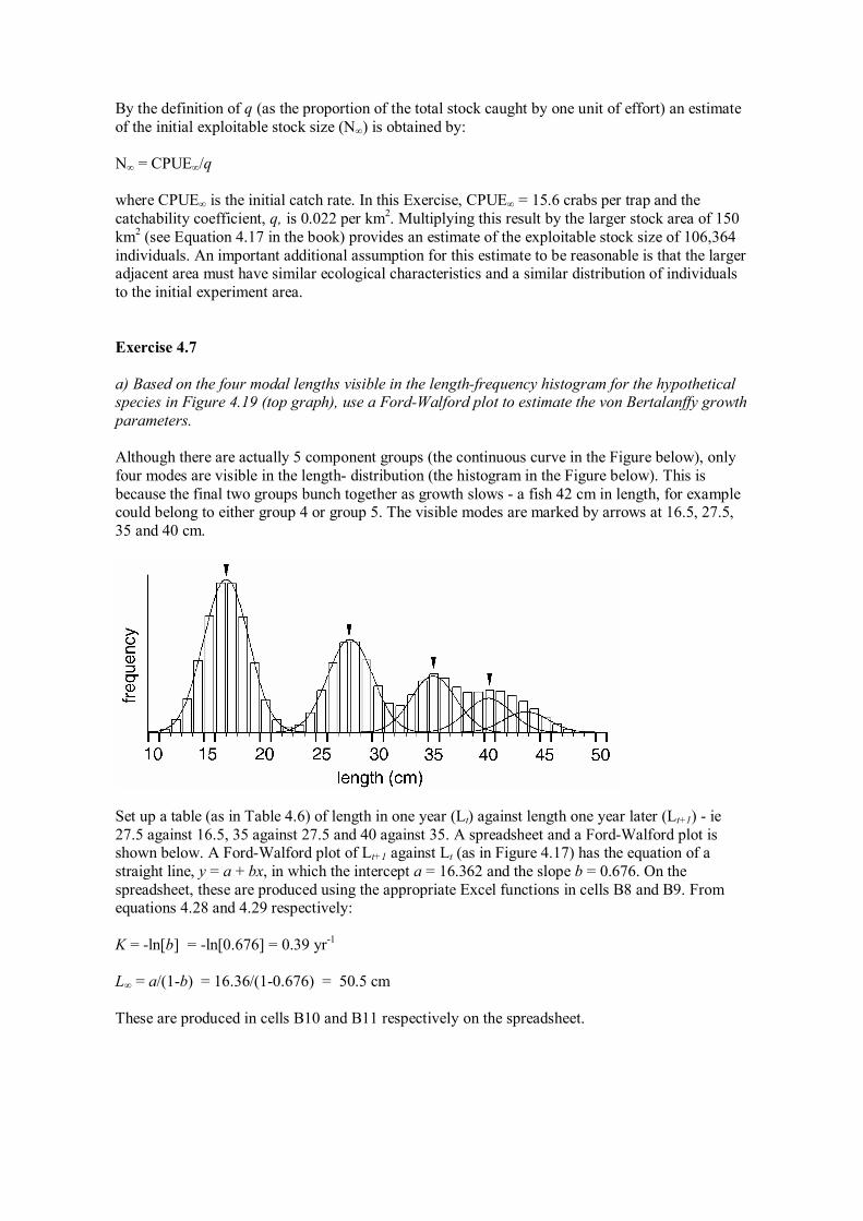
a) Based on the four modal lengths visible in the length­frequency histogram for the hypothetical species in Figure 4.19 (top graph), use a Ford­Walford plot to estimate the von Bertalanffy growth parameters.

Although there are actually 5 component groups (the continuous curve in the Figure below), only four modes are visible in the length­ distribution (the histogram in the Figure below). This is because the final two groups bunch together as growth slows ­ a fish 42 cm in length, for example could belong to either group 4 or group 5. The visible modes are marked by arrows at 16.5, 27.5, 35 and 40 cm.

Set up a table (as in Table 4.6) of length in one year (Lt) against length one year later (Lt+1) ­ ie 27.5 against 16.5, 35 against 27.5 and 40 against 35. A spreadsheet and a Ford­Walford plot is shown below. A Ford­Walford plot of Lt+1 against Lt (as in Figure 4.17) has the equation of a straight line, y = a + bx, in which the intercept a = 16.362 and the slope b = 0.676. On the spreadsheet, these are produced using the appropriate Excel functions in cells B8 and B9. From equations 4.28 and 4.29 respectively:

K = ­ln[b] = ­ln[0.676] = 0.39 yr ­1

L∞ = a/(1­b) = 16.36/(1­0.676) = 50.5 cm

These are produced in cells B10 and B11 respectively on the spreadsheet.

Ford­Walford plot

Lt Lt+1 16.5 27.5 27.5 35 35 40

slope = 0.68 intercept = 16.36

K = 0.39 L infinity = 50.52

y = 0.6761x + 16.362

0

10

20

30

40

50

0 10 20 30 40 50

length at year t

length a

t year t+1

b) Use the estimated parameters K and L∞ (and assume to=0) in the von Bertalanffy equation to predict fish length for ages from 0 to 8 years (an age­length key) in steps of 0.5 years and draw a growth curve.

An age­length key can be prepared by estimating length, L, for a range of arbitrarily selected ages, t. The von Bertalanffy equation (Equation 4.22 in the book) is:

Lt = L∞(1­exp[­K(t­to)])

where Lt is the length at age t, L∞ is the asymptotic length of 50.5 cm and K is the growth coefficient, 0.39 yr ­1 . The age at zero length (to) is assumed to be zero (ie the graph passes through the origin). A sample spreadsheet table is shown below based on the parameters K, L infinity (L∞ ) and t zero (to ) that are included in cells B2, B3 and B4 respectively. A growth curve is a plot of length values (L) in column 2 against age (t) in column 1 using the Excel formula $B$3*(1­EXP(­ $B$2*(A7­ $B$4))) typed in cell B7 and copied down to B17.

Age­length key and growth curve using L=Linf(1­exp[­K(t­tzero)]) K = 0.39

Linf = 50.5 t zero = 0

age, t length, L 0 0.0 1 16.3 2 27.4 3 34.8 4 39.9 5 43.3 6 45.6 7 47.2 8 48.3 9 49.0 10 49.5

0 5 10 15 20 25 30 35 40 45 50 55

0 2 4 6 8 10 age, t

length

, L

c) Estimate the approximate mean life­span of the fish as the age at which the species reaches 95% of the value of L∞; use the inverse of the von Bertalanffy formula (i.e. make age, t, the subject of Equation 4.22).

If mean lifespan (tmax) is roughly the time required for a fish to reach 95% of its asymptotic length, L∞, then from the inverse of the von Bertalanffy growth equation (Equation 4.22):

tmax =(­1/K) ln[1­(0.95L∞)/L∞] or approximately, tmax = 3/K

Using the growth parameters estimated in the first part, this equation (given in Chapter 4 as Equation 4.74) provides an approximate lifespan of 7.7 years. If the species lives for over 7 years, why are there only 4 or 5 size groups in the length­frequency histogram given? One common reason is that the species is heavily exploited and larger individuals are rare or absent.

Exercise 4.8

The numbers given in the exercise are the lengths (cm) of 221 fish caught in a single tow of a trawl net. Display the length­frequency data as a histogram similar to that shown in Figure 4.21. From the left, label the four modal (highest) points on the graph as 0+ years, 1+ years, 2+ years, and 3+ years.

The completed histogram should be similar to the one below with modes at 12, 28, 39, and 46 cm.

c) Use the modal values to draw a graph of length at age t+1 against length at age t (a Ford­ Walford plot with three points, similar to that shown in Figure 4.17) in order to estimate K and L∞.

A Ford­Walford plot of Lt+1 against Lt is similar to that completed in the previous exercise and shown in Figure 4.17 in the book. The equation the straight line fitting the data has an intercept a = 20.1 and a slope b = 0.67. From equations 4.28 and 4.29:

K = ­ln[b] = 0.4 yr ­1

L∞ = a/(1­b) = 60.9 cm

d) Use the values of K and L∞ to predict fish length for a range of ages (assume to = 0). Enter the estimated lengths in an age length key and draw a von Bertalanffy growth curve.

An age­length key can be prepared as in the previous Exercise by substituting the values of K and L∞ in the von Bertalanffy equation (Equation 4.22 in the book) for a range of arbitrarily selected ages, t. As the age at zero length is assumed to be zero, the growth curve will pass through the origin.

e) Examine the above procedure carefully. What aspects of the biology of this hypothetical fish species could result in the estimates of K and L∞ being quite wrong?

The initial assumption is that the sample shown in the histogram is representative of the actual population ­ that is, the gear used to collect the sample was totally unselective (whereas, in fact, all fishing gear is selective to some extent). By labelling the modes as 0+, 1+, 2+ and 3+, the assumption is that the modes represent successive age classes produced by spawning events that were 12 months apart. If the species spawned irregularly, or at intervals of more or less than one year, the results would be incorrect.

Exercise 4.9

The heights of a large and random sample of humans could be plotted as a length­frequency graph as used to analyse growth in some fish populations. But it is impossible to use such a graph to estimate the growth of humans from the relative frequencies in size classes. Why is this so?

Humans breed more or less evenly over the year. A length­frequency distribution would therefore show no separate age­classes and be something like the lower histogram in Figure 4.19 for a fish stock with an extremely extended spawning season.

Exercise 4.10

Re­analyse the penaeid prawn data in Table 4.9 to estimate K using a "forced" Gulland­Holt plot with L∞ = 46 mm carapace length (ignore negative growth increments).

The data (mean lengths and corresponding growth rates) can be entered on a spreadsheet as shown below. In a "forced" Gulland­Holt plot, the mean growth­rate and the mean length are used, and these values are calculated at the bottom of columns A and B. In this case forcing the line through a fixed value of L∞ on the X­axis (46 mm in this case) gives an approximate value for K as .

forcedK = meanY /(forcedL∞ ­ meanX) = 0.21/(46 ­ 37.85) = 0.025 week ­1

The “forced” straight line that cuts the X­axis at 46 mm is of the formY = forcedK (forcedL∞ ­ x) and this equation is entered in column C. This column is used to produce the “forced” line on the graph and the Excel “trendline” function is used to create the “unforced” or best fitting line through the data in column B.

Gulland­Holt plot (with best fit and "forced" solutions) meanL growth rate forced

31.1 0.34 0.38 32.5 0.37 0.34 33.2 0.3 0.33 33.4 0.28 0.32 34.1 0.31 0.30 37.8 0.21 0.21 36.6 0.15 0.24 36.3 0.26 0.25 37.6 0.13 0.21 39.6 0.12 0.16 38.5 0.12 0.19 40.4 0.18 0.14 42.2 0.19 0.10 43.6 0.13 0.06 43.3 0.07 0.07 45.4 0.16 0.02 best fit Linf = 50 best fit K = 0.017 37.85 0.21 < means forced Linf = 46 forced K = 0.025

y = ­0.017x + 0.851

0

0.1

0.2

0.3

0.4

30 35 40 45 50 length

grow

th rate

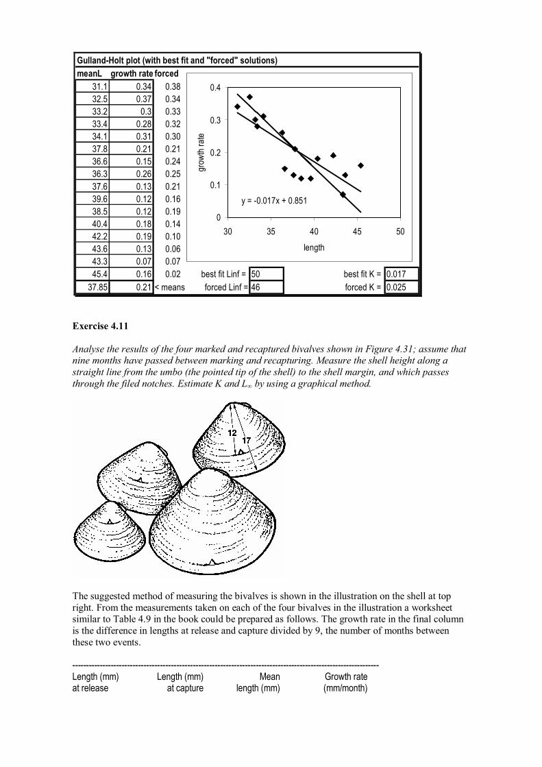
Exercise 4.11

Analyse the results of the four marked and recaptured bivalves shown in Figure 4.31; assume that nine months have passed between marking and recapturing. Measure the shell height along a straight line from the umbo (the pointed tip of the shell) to the shell margin, and which passes through the filed notches. Estimate K and L∞ by using a graphical method.

The suggested method of measuring the bivalves is shown in the illustration on the shell at top right. From the measurements taken on each of the four bivalves in the illustration a worksheet similar to Table 4.9 in the book could be prepared as follows. The growth rate in the final column is the difference in lengths at release and capture divided by 9, the number of months between these two events.

­­­­­­­­­­­­­­­­­­­­­­­­­­­­­­­­­­­­­­­­­­­­­­­­­­­­­­­­­­­­­­­­­­­­­­­­­­­­­­­­­­­­­­­­­­­­­­­­­­­­­­­­­­­­­­­­ Length (mm) Length (mm) Mean Growth rate at release at capture length (mm) (mm/month)

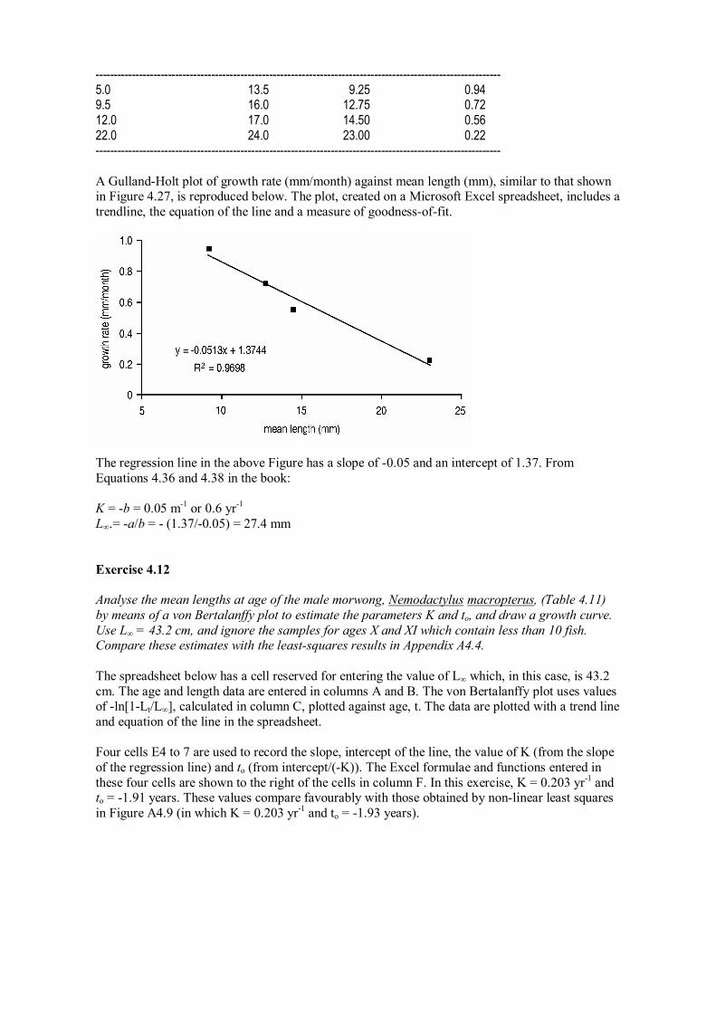
­­­­­­­­­­­­­­­­­­­­­­­­­­­­­­­­­­­­­­­­­­­­­­­­­­­­­­­­­­­­­­­­­­­­­­­­­­­­­­­­­­­­­­­­­­­­­­­­­­­­­­­­­­­­­­­­ 5.0 13.5 9.25 0.94 9.5 16.0 12.75 0.72 12.0 17.0 14.50 0.56 22.0 24.0 23.00 0.22 ­­­­­­­­­­­­­­­­­­­­­­­­­­­­­­­­­­­­­­­­­­­­­­­­­­­­­­­­­­­­­­­­­­­­­­­­­­­­­­­­­­­­­­­­­­­­­­­­­­­­­­­­­­­­­­­­

A Gulland­Holt plot of growth rate (mm/month) against mean length (mm), similar to that shown in Figure 4.27, is reproduced below. The plot, created on a Microsoft Excel spreadsheet, includes a trendline, the equation of the line and a measure of goodness­of­fit.

The regression line in the above Figure has a slope of ­0.05 and an intercept of 1.37. From Equations 4.36 and 4.38 in the book:

K = ­b = 0.05 m ­1 or 0.6 yr ­1 L∞.= ­a/b = ­ (1.37/­0.05) = 27.4 mm

Exercise 4.12

Analyse the mean lengths at age of the male morwong, Nemodactylus macropterus, (Table 4.11) by means of a von Bertalanffy plot to estimate the parameters K and to, and draw a growth curve. Use L∞ = 43.2 cm, and ignore the samples for ages X and XI which contain less than 10 fish. Compare these estimates with the least­squares results in Appendix A4.4.

The spreadsheet below has a cell reserved for entering the value of L∞ which, in this case, is 43.2 cm. The age and length data are entered in columns A and B. The von Bertalanffy plot uses values of ­ln[1­Lt/L∞], calculated in column C, plotted against age, t. The data are plotted with a trend line and equation of the line in the spreadsheet.

Four cells E4 to 7 are used to record the slope, intercept of the line, the value of K (from the slope of the regression line) and to (from intercept/(­K)). The Excel formulae and functions entered in these four cells are shown to the right of the cells in column F. In this exercise, K = 0.203 yr ­1 and to = ­1.91 years. These values compare favourably with those obtained by non­linear least squares in Figure A4.9 (in which K = 0.203 yr ­1 and to = ­1.93 years).

von Bertalanffy plot Linf = 43.2 << enter L infinity here

age length Lt/Linf] 3 27.2 0.993 slope = 0.203 << SLOPE(C4:C10,A4:A10) 4 30.3 1.209 intercept = 0.388 << INTERCEPT(C4:C10,A4:A10) 5 32.6 1.405 K = 0.203 << E4 6 34.6 1.614 tzero = 1.912 << E5/E4 7 35.9 1.778 8 37.3 1.991 9 38.6 2.240 10 40.6 2.810 < data not included in plot 11 42.5 4.123 < data not included in plot

y = 0.2028x + 0.3877 R 2 = 0.9981

0.0

0.5

1.0

1.5

2.0

2.5

2 3 4 5 6 7 8 9 10

Exercise 4.13

a) Use the drawing of the bivalve, Vasticardium, in Figure 4.28 to estimate K and L∞ in the von Bertalanffy growth equation.

Using the scale provided on Figure 4.28, there are bands at 13, 22, 28, 32, 35 and 37 mm. To use a Ford­Walford plot, the data could be organized in a similar way to Table 4.6 as follows:

­­­­­­­­­­­­­­­­­­­ Lt Lt+1 ­­­­­­­­­­­­­­­­­­­ 13 22 22 28 28 32 32 35 35 37 ­­­­­­­­­­­­­­­­­­­

A Ford­Walford plot of Lt+1 against Lt (as in Figure 4.17) has the equation of a straight line, y = a + bx, in which the intercept a = 13.04 and the slope b = 0.683. From equations 4.28 and 4.29:

K = ­ln[b] = ­ln[0.683] = 0.38 yr ­1

L∞ = a/(1­b) = 13.04/(1 ­ 0.683) = 41.1 mm

b) If the bivalve was collected in mid­June, and the species is known to reach a spawning peak in mid September, estimate to.

Making to the subject of the von Bertalanffy growth equation (Equation 4.22) gives:

to = t + (1/K)(ln[(L∞­Lt)/L∞])

as given in Equation 4.30 of the book. If the individual resulted from a mid­September spawning it would have been 13 mm by the following mid­June, 9 months later. Substituting K = 0.38 yr ­1 , and L∞ = 41.1 mm and the age and length of the first modal group (t = 0.75 years and Lt = 13 mm respectively) provides an estimate of to = ­ 0.25 years.

c) Draw the growth curve for the species based on this one individual. Comment on whether or not this is reasonable, and consider the assumptions that the above analyses rely on.

A growth curve can be constructed by substituting the values of K, L∞ and to.in the growth equation Lt = L∞ (1 ­ exp[­K(t­t0)]) given as Equation 4.22 in the book. That is by calculating values of Lt for a range of ages, say from t = 0 to 8 in steps of 1 year.

An alternative and more direct way of obtaining parameter estimates to construct a growth curve is to adapt the computer program suggested in Figure A4.6 in Appendix 4. The output of the program is shown below) has minimized the SSR of 0.034 with K = 0.38 yr ­1 , L∞ = 41.2 cm and t0 = ­ 007 years. Other than the value obtained for t0 the values of the other two parameters compare favourably with those obtained by the graphical method.

It is, of course, unreasonable to expect the growth curve based on this one individual to represent growth in the entire population. Within all species there are differences in growth rates between individuals. In addition, the analysis, assumes that the rings were laid down at yearly intervals.

Growth ­ fitting a curve to length­at­age K > 0.37799

Linf > 41.1997 age length tzero > ­0.0069 0 0.11

1 13.04 age L obs L exp SR 2 21.90

1 13.0 13.04 0.002 3 27.98 2 22.0 21.90 0.009 4 32.14 3 28.0 27.98 0.000 5 34.99 4 32.0 32.14 0.019 6 36.95 5 35.0 34.99 0.000 7 38.28 6 37.0 36.95 0.003 8 39.20

SSR> 0.034 9 39.83 10 40.26

0 5

10 15 20 25 30 35 40 45

0 2 4 6 8

age (years)

length (cm

)

Exercise 4.14

The table below shows the numbers of fish caught per unit of effort in each of three age classes. Fish more than one year old are sexually mature and immature fish are recruited to the adult stock before they are 12 months of age. Use these data to estimate a stock­recruitment relationship.

The table given in the exercise can be rearranged into columns that represent newly­recruited individuals and reproductive individuals (age classes 1+ and 2+) and the resulting recruitment (0+

in the FOLLOWING year); that is, a mature stock of 402 individuals in 1985 resulting in a recruitment of 210 individuals in 1986 etc as follows:

­­­­­­­­­­­­­­­­­­­­­­­­­­­­­­­­­­­­­­­­­­­­­­­­­­­­­­­­­­­­­­­­­­­­­­­­­­­­­­­­ year stock recruitment in the

(1+ and 2+) following year (0+) ­­­­­­­­­­­­­­­­­­­­­­­­­­­­­­­­­­­­­­­­­­­­­­­­­­­­­­­­­­­­­­­­­­­­­­­­­­­­­­­­ 1985 402 210 1986 183 255 1987 240 270 1988 141 195 1989 130 180 ­­­­­­­­­­­­­­­­­­­­­­­­­­­­­­­­­­­­­­­­­­­­­­­­­­­­­­­­­­­­­­­­­­­­­­­­­­­­­­­­

A stock­recruitment curve can be drawn by eye through a scatter plot of these values. Alternatively the data may be entered in a Microsoft Excel spreadsheet and the routine Solver can be used to produce curves as shown in Appendix 4.6. The spreadsheet shown below is adapted from Figure A4.11 in Appendix 4.6.

The Ricker model, in which recruitment (R) reaches a maximum before decreasing at higher levels of stock abundance (S), is R = a S exp(­bS). The Beverton and Holt model, in which recruitment approaches an asymptote at high stock densities, is R = aS/(b+S). Solver is used to find values for a and b in the Ricker model and then, separately, to find the values of a and b in the Beverton and Holt model (a and b in each model are unrelated). These values are used to predict recruitment over a range of stock levels for the Ricker model (column H) and for the Beverton & Holt model (column I). These columns are the bases of the curves in the graph on which the five raw data points (from column B) have been superimposed.

stock­recruitment curves Ricker B&H Ricker B&H stock curve curve

a> 2.46742 a> 275.1592 0 0 0 b> 0.00371 b> 47.93834 25 56 94

50 102 140 stock recruit Rick.log SR B&H log SR 75 140 168 130 180 0.421 0.009 0.436 0.012 100 170 186 141 195 0.380 0.003 0.376 0.003 125 194 199 183 255 0.224 0.012 0.175 0.025 150 212 209 240 270 0.013 0.011 ­0.045 0.027 175 226 216 402 210 ­0.588 0.004 ­0.492 0.025 200 235 222

SSR> 0.039 SSR> 0.091 225 241 227 250 244 231 275 245 234 300 243 237 325 240 240 350 236 242 375 230 244 400 224 246 425 217 247 450 209 249 475 201 250 500 193 251 525 185 252 550 176 253 575 168 254

0

50

100

150

200

250

300

0 200 400 600

Exercise 4.15

Prepare a graph relating instantaneous mortality rates to percentage mortality rates (place percentage rates from 0 to 90 on the X­axis).

Percentage mortalities are related to instantaneous mortality rates by Equation 4.53 in Chapter 4:

Mortality (%) = 100 (1­exp[­Z])

Percentage mortality rates from 0 to 90 are entered in column A. Making Z the subject of the above equation gives Z = ln[1­ (% mortality)/100], which is entered in column B of the spreadsheet.

% Z 0 0.00 5 0.05 10 0.11 15 0.16 20 0.22 25 0.29 30 0.36 35 0.43 40 0.51 45 0.60 50 0.69 55 0.80 60 0.92 65 1.05 70 1.20 75 1.39 80 1.61 85 1.90 90 2.30

0.00

0.50

1.00

1.50

2.00

2.50

0 10 20 30 40 50 60 70 80 90 % mortality

instant mo

rtality

(z)

Exercise 4.16

Estimate the growth parameters, K and L∞, and the total mortality, Z, from the length­frequency data shown in the figure. List the separate assumptions that estimating growth and mortality in this way depend on.

The figure below has had the numbers in each length class added to the top of each column and the three modes are indicated by arrows. The estimation of growth depends on the positions of the modes and the estimation of mortality depends on the numbers within each of the three size groups ­ the use of each depends on separate conditions.

The modes occur at the middle of size classes at 23.5, 33.5 and 40.5 cm. The numbers within each of the size classes are totalled. Here the selection of cut­off points (between size classes) is somewhat arbitrary ­ if the cut­off point between the second and third size class, for example, is taken to be 37.5 cm half of the numbers in the size class from 37 to 38 should be regarded as belonging to the second size class and half to the third size class. Details can be arranged as in the table below.

­­­­­­­­­­­­­­­­­­­­­­­­­­­­­­­­­­­­­­­­­­­­­­­­­­­­­­­­­­­­­­­­­­­­­­­­­­­­­­­­­­­­­ class modal length numbers ln[number] ­­­­­­­­­­­­­­­­­­­­­­­­­­­­­­­­­­­­­­­­­­­­­­­­­­­­­­­­­­­­­­­­­­­­­­­­­­­­­­­­­­­­­ 1 23.5 162.5 5.09 2 33.5 96.0 4.56 3 40.5 46.5 3.84 ­­­­­­­­­­­­­­­­­­­­­­­­­­­­­­­­­­­­­­­­­­­­­­­­­­­­­­­­­­­­­­­­­­­­­­­­­­­­­­­­­­­­­

The modal lengths can be used to estimate growth using the program described in Figure A4.3 in Appendix 4 of the book. A misleadingly good fit is obtained using only three points. To approximate reality the key assumption is that each of the three modes represents size classes that have been produced from spawning events separated by one year.

Growth ­ fitting a curve to length­at­age K > 0.36

Linf > 56.83 age length tzero > ­0.50 0 9.2

1 23.5 age L obs L exp SR 2 33.5

1 23.5 23.50 0.000 3 40.5 2 33.5 33.50 0.000 4 45.4 3 40.5 40.50 0.000 5 48.8

SSR> 0.000 6 51.2 7 52.9 8 54.1 9 54.9

0 10 20 30 40 50 60

0 1 2 3 4 5 6 age (years)

leng

th (c

m)

Plotting the natural logarithms of numbers in each size class as a catch curve (as in Figure 4.44) gives a slope and therefore an estimate of total mortality, Z, as 0.63 per year. For this estimate to be reasonable, the same number of juveniles would have to have been recruited in each of the years that produced the three size classes. This situation is unlikely as environmental fluctuations alone must result in annual recruitment that is highly variable in most species. However, if a much larger number of points was available, and recruitment varied randomly, a catch curve may

produce a reasonable estimate of average mortality. An important additional assumption is that all size classes are equally vulnerable to the fishing gear.

Exercise 4.17

A biologist has access to records from a processing factory as shown below. The factory grades the prawn catch as the number of prawns per kg and the table shows the catches and grade landed in the four months immediately following recruitment. Make an initial estimate of the total instantaneous mortality rate, Z, and list the important assumptions that must apply for the estimate to be a reasonable one.

The table given in the Exercise can be extended as follows: ­­­­­­­­­­­­­­­­­­­­­­­­­­­­­­­­­­­­­­­­­­­­­­­­­­­­­­­­­­­­­­­­­­­­­­­­­­­­­­­­­­­­­­­­­­­­­­­­­­­­­­­­­­­­­­­­­ month numbers catch numbers ln(numbers)

(per kg) (kg) ­­­­­­­­­­­­­­­­­­­­­­­­­­­­­­­­­­­­­­­­­­­­­­­­­­­­­­­­­­­­­­­­­­­­­­­­­­­­­­­­­­­­­­­­­­­­­­­­­­­­­­­­­­­­­­­­­ 1 35 5690 199150 12.20 2 28 5260 147280 11.90 3 24 4550 109200 11.60 4 22 3670 80740 11.30 ­­­­­­­­­­­­­­­­­­­­­­­­­­­­­­­­­­­­­­­­­­­­­­­­­­­­­­­­­­­­­­­­­­­­­­­­­­­­­­­­­­­­­­­­­­­­­­­­­­­­­­­­­­­­­­­­­

A regression of the natural logarithm against month is a catch curve that, in this example, estimates total mortality, Z, at 0.3 per month. For the estimate to be reasonable fishing effort in each of the four months would have had to be similar and prawns of all sizes would have to be equally susceptible to the fishing gear. In addition, there must be no movement of prawns into or out of the area fished.

Exercise 4.18

A clupeid fish species is recruited at an age of 5 months when it is fully vulnerable to the fishing gear. Mean catch rates per month, starting at the month of recruitment, are 145, 215, 295, 380, and 466 kg/hour. Growth is described by the von Bertalanffy growth equation with K=0.05 (m ­1 ), and L∞ =35 cm. Weight (g) is related to length (cm) by a power curve with a=0.03 and b=3. Estimate the total mortality rate (Z) for the species. List the assumptions that must be accepted for the estimate to be a reasonable one.

The calculations can organized as in the following table. In the third column, length is estimated by the von Bertalanffy growth equation by substituting the values of K, and L∞ (assuming t0 = 0) in the growth equation Lt = L∞ (1 ­ exp[­Kt]) given as Equation 4.22 in the book. In the fourth column, weight is predicted using Equation 4.20 in the book in which weight (W) is related to length (L) by W = aL b . CPUE can now be converted from weight units to numbers caught per hour.

­­­­­­­­­­­­­­­­­­­­­­­­­­­­­­­­­­­­­­­­­­­­­­­­­­­­­­­­­­­­­­­­­­­­­­­­­­­­­­­­­­­­­­­­­­­­­­­­­­­­­­­­­­­­­­­­­­­­­­­­­­­­­­­­­­­­­­ month CPUE (kg) length (cm) weight (g) CPUE (nos) ln CPUE ­­­­­­­­­­­­­­­­­­­­­­­­­­­­­­­­­­­­­­­­­­­­­­­­­­­­­­­­­­­­­­­­­­­­­­­­­­­­­­­­­­­­­­­­­­­­­­­­­­­­­­­­­­­­­­­­­­­­­­­­­­­­­­­­­­­­­­ 5 145 7.74 13.91 10424 9.25 6 215 9.07 22.38 9607 9.17 7 295 10.34 33.17 8894 9.09 8 380 11.54 46.10 8243 9.02 9 466 12.68 61.16 7619 8.94 ­­­­­­­­­­­­­­­­­­­­­­­­­­­­­­­­­­­­­­­­­­­­­­­­­­­­­­­­­­­­­­­­­­­­­­­­­­­­­­­­­­­­­­­­­­­­­­­­­­­­­­­­­­­­­­­­­­­­­­­­­­­­­­­­­­­­­­

A regression line through the natural logarithms in the final column has a slope of ­0.078 which suggests a total mortality rate, Z, of 0.078 per month. Key assumptions are that there is no further recruitment and individuals are not migrating either into or away from the fishing grounds.

Exercise 4.19

Catch (t) and effort (hours trawled) by month for a penaeid prawn, Penaeus latisulcatus, trawl fishery are shown in the table below. Recruitment is assumed to be complete by March when the newly­recruited prawns are 6 months of age. The von Bertalanffy equation applies to growth with K = 0.15 m ­1 and L∞=55 mm. Weight (g) is related to carapace length (mm) by the equation W = 0.0005 L 3 . Examine the use of the data in a catch curve to estimate mortality. There is some evidence that prawns spend more time under the substrate in colder months (southern hemisphere winter months), and may be less accessible to the trawl gear.

The Table given in this Exercise can be extended as suggested in Table 4.18 or as part of a spreadsheet as shown below. In column E of the spreadsheet, carapace length is predicted by the von Bertalanffy growth equation as 55*(1­exp[­0.15*t]) where t is age picked up from column B. In column F, individual weight is 0.0005*(L^3) where L is length picked up from column E. In column G, the number of individuals in the catch is calculated as C*(1000^2)/W where C is the catch weight from column C and W is individual weight from column F ­ note that tonnes have to be converted to grams. In column H, CPUE in number caught per hour is calculated as C/f where C is from column G and f (effort) is picked up from column D. In the final column, CPUE is converted to natural logarithms.

A B C D E F G H I month age catch effort length weight catch CPUE ln[CPUE]

(m) (tonnes) (hr) (mm) (g) (numbers) (nos/hr) (nos/hr) JAN 4 169.1 3068 24.8 7.6 22131552 7214 8.88 FEB 5 252.9 4738 29.0 12.2 20696352 4368 8.38 MAR 6 298.6 4146 32.6 17.4 17176018 4143 8.33 APR 7 314.2 5171 35.8 22.9 13749385 2659 7.89 MAY 8 173.9 3974 38.4 28.4 6125930 1542 7.34 JUN 9 79.5 2388 40.7 33.8 2351132 985 6.89 JUL 10 45.8 1693 42.7 39.0 1174256 694 6.54 AUG 11 45.8 1858 44.4 43.9 1043888 562 6.33 SEP 12 62.5 2383 45.9 48.4 1291900 542 6.30 OCT 13 69.4 2738 47.2 52.5 1322074 483 6.18 NOV 14 164.7 4431 48.3 56.2 2929743 661 6.49 DEC 15 59.8 2024 49.2 59.6 1004050 496 6.21

y = ­0.2546x + 9.5655

5

6

7

8

9

4 6 8 10 12 14 16 age (months)

ln [CPU

E] (n

umbers per hour)

The slope of the catch curve in the above spreadsheet graph provides an estimate of total mortality, Z of 0.26 per month. However, the straight line does not fit the data that well ­ possibly because

the prawns are less accessible to the gear in the Southern Hemisphere winter months from June to August. This suggests that data from these months should be excluded from the analysis; on the other hand, the removal of the three winter points (for ages 9, 10 and 11 months) may not make that much difference to the slope of the catch curve. Try it and see.

Exercise 4.20

When analysing mark­recapture data from a single release of tagged fish, what would be the effects on estimates of total and natural mortality if a) a constant 10% of tagged fish caught are unreported by fishers, and b) fishers gradually lose interest in returning tagged fish due to poor feedback from researchers?

Details for this Exercise are given in Box 4.13 in Chapter 4 of the book. If a constant 10% of tagged fish caught are unreported by fishers, the slope of the line in Figure B4.13.1 will not be affected but the intercept on the y­axis will. Hence, the analysis will provide an accurate estimate of total mortality, Z, but an inaccurate estimate of fishing mortality, F and therefore also natural mortality, M.

If fishers gradually lose interest in returning tagged fish due to poor feedback from researchers the slope of the line will be steeper and Z will be overestimated. However, the intercept on the y­axis will be unaffected and estimates of F and M will be reasonable.

Exercise 4.21

The length­frequency diagram shown in the figure is from a sample of scad, Decapterus macrosoma, caught in a purse­seine net during surveys. Growth is described by the von Bertalanffy growth equation with K= 0.8 yr ­1 and L∞ = 38.3 cm. Estimate the total mortality rate (Z) for the species. Accepting that the growth parameters are correct, list assumptions that must be made for the estimate to be a reasonable one.

The length­frequency distribution above has to be converted to an age­frequency distribution before a catch­curve can be used to estimate mortality. This is the basis of a length­converted catch curve shown in Figure 4.47 and a spreadsheet model produced by the spreadsheet program presented in Appendix A4.7 “Length­converted catch curve ­ lobster example.”

Length­converted catch curve K > 0.8 first point > 0.9 slope > ­1.704 Linf 38.3last point > 2.5 Z > 1.704

age age age at ln[F/dt] ln[F/dt] L1 L2 mid L F at L1 change mid L regress.

15 17 16 23 0.621 0.1122 0.676 5.32 17 19 18 96 0.733 0.1233 0.794 6.66 19 21 20 174 0.857 0.1367 0.923 7.15 7.15 21 23 22 162 0.993 0.1536 1.068 6.96 6.96 23 25 24 128 1.147 0.1751 1.231 6.59 6.59 25 27 26 120 1.322 0.2037 1.420 6.38 6.38 27 29 28 98 1.526 0.2435 1.642 6.00 6.00 29 31 30 70 1.769 0.3027 1.911 5.44 5.44 31 33 32 54 2.072 0.4002 2.256 4.90 4.90 33 35 34 22 2.472 0.5922 2.734 3.61 35 37 36 6 3.064

y = ­1.7041x + 8.7485

0 1 2 3 4 5 6 7 8

0.02 0.52 1.02 1.52 2.02 2.52 3.02 relative age

ln[F/dt]

The regression line is fitted through the data from the final column. The line is through data which excludes the initial ascending data points representing groups of individuals which are either not fully recruited or are too small to be totally vulnerable to the fishing gear, and data points close to L∞, where the relationship between length and age becomes uncertain.

The value of total mortality estimated from the slope of the length­converted catch curve shown below is Z = 1.7 yr ­1 . Note that growth and mortality rates are very high in many small tropical clupeids.

Exercise 4.22

A fish species grows according to the von Bertalanffy growth equation with K = 0.4 yr ­1 and L∞ = 60 cm, and the mean length at first capture is 18 cm. Over several years of increasing effort, the mean size of fish in the catch has been decreasing as shown in the table below. Estimate the natural mortality rate, M.

Total mortality, Z, can be calculated using Equation 4.61 in the book by:

Z =K [(L∞ ­ Lc)/(Lc ­ Lc)]

where Lc is the mean length at first capture, and Lc is the mean length of fish in the catch. The data provided can be entered on a spreadsheet as shown below. In column D, Z is estimated by substituting the growth parameters provided in the above Equation.

Total and natural mortality

K= 0.4 Linf = 60 Lc = 18

year effort mean total (hours) length (cm) mortality,Z

1 1760 34.8 0.60 2 2800 33.2 0.71 3 3640 32.1 0.79 4 4120 31.7 0.83 5 4680 31.2 0.87

y = 9E­05x + 0.4396

0.0

0.2

0.4

0.6

0.8

1.0

0 1000 2000 3000 4000 5000 effort (hours)

tota

l mor

talit

y The straight line through the data is extrapolated back to the y­axis where the fishing effort is zero and therefore fishing mortality, F = 0. At this point on the x­axis, total mortality is equivalent to natural mortality. That is, M is equivalent to the intercept on the Y­axis, which in this case is 0.44.

­­­­­­­­­­­­­­­­­­­­­­­­­­­­­­­­­­­­­­­­­­­­­­­­­­­­­­­­­­­­­­­­­­­­­­­­­­­­­­­­­­­­­­­­­­­­­­­­­­­­­­

Chapter 5. Stock assessment

This Chapter aims to familiarize the reader with methods used in the assessment of fish stocks. Equilibrium and non­equilibrium models, classical yield per recruit models, simulation models and ecosystem models are described and worked examples provided. Appendix A4 of the book contains step­by­step instructions on building computer spread sheet models for stock assessment, including simulation models and risk assessment models

Exercise 5.1

Deepwater snappers are caught by artisanal fishers using handreels and droplines in depths of over 200m off many tropical coasts. The approximate fishing effort (in trips per year) and the combined catch of two deepwater snapper species, Etelis and Pristipomoides, are shown below. Estimate fishing effort to secure the maximum sustainable yield, fMSY, using both the Schaefer and Fox models.

The table provided in this Exercise can be extended in a similar way to Table 5.1 as follows. ­­­­­­­­­­­­­­­­­­­­­­­­­­­­­­­­­­­­­­­­­­­­­­­­­­­­­­­­­­­­­­­­­­­­­­­­­­­­­­­­­­­­­­­­­­­­­­­­­­­­­­­­­­­­­ Effort (trips) Catch (kg) CPUE (kg/trip) ln CPUE ­­­­­­­­­­­­­­­­­­­­­­­­­­­­­­­­­­­­­­­­­­­­­­­­­­­­­­­­­­­­­­­­­­­­­­­­­­­­­­­­­­­­­­­­­­­­­­­­­­­­­­­­­­­­­ 106 60000 566.04 6.34 215 86000 400.00 5.99 321 110000 342.68 5.84 491 136000 276.99 5.62 540 176000 325.93 5.79 608 141000 231.91 5.45 650 155000 238.46 5.47 680 141000 207.35 5.33 885 180000 203.39 5.32 920 208000 226.09 5.42 1100 178000 161.82 5.09 1410 160000 113.48 4.73

­­­­­­­­­­­­­­­­­­­­­­­­­­­­­­­­­­­­­­­­­­­­­­­­­­­­­­­­­­­­­­­­­­­­­­­­­­­­­­­­­­­­­­­­­­­­­­­­­­­­­­­­­­­­­

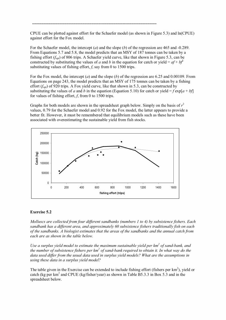
CPUE can be plotted against effort for the Schaefer model (as shown in Figure 5.3) and ln(CPUE) against effort for the Fox model.

For the Schaefer model, the intercept (a) and the slope (b) of the regression are 465 and ­0.289. From Equations 5.7 and 5.8, the model predicts that an MSY of 187 tonnes can be taken by a fishing effort (fopt) of 806 trips. A Schaefer yield curve, like that shown in Figure 5.3, can be constructed by substituting the values of a and b in the equation for catch or yield = af + bf 2 substituting values of fishing effort, f, say from 0 to 1500 trips.

For the Fox model, the intercept (a) and the slope (b) of the regression are 6.25 and 0.00109. From Equations on page 243, the model predicts that an MSY of 175 tonnes can be taken by a fishing effort (fopt) of 920 trips. A Fox yield curve, like that shown in 5.3, can be constructed by substituting the values of a and b in the equation (Equation 5.10) for catch or yield = f exp[a + bf] for values of fishing effort, f, from 0 to 1500 trips.

Graphs for both models are shown in the spreadsheet graph below. Simply on the basis of r 2 values, 0.79 for the Schaefer model and 0.92 for the Fox model, the latter appears to provide a better fit. However, it must be remembered that equilibrium models such as these have been associated with overestimating the sustainable yield from fish stocks.

0

50000

100000

150000

200000

250000

0 200 400 600 800 1000 1200 1400 1600

fishing effort (trips)

Catc

h (k

g)

Exercise 5.2

Molluscs are collected from four different sandbanks (numbers 1 to 4) by subsistence fishers. Each sandbank has a different area, and approximately 60 subsistence fishers traditionally fish on each of the sandbanks. A biologist estimates that the areas of the sandbanks and the annual catch from each are as shown in the table below.

Use a surplus yield model to estimate the maximum sustainable yield per km 2 of sand­bank, and the number of subsistence fishers per km 2 of sand­bank required to obtain it. In what way do the data used differ from the usual data used in surplus yield models? What are the assumptions in using these data in a surplus yield model?

The table given in the Exercise can be extended to include fishing effort (fishers per km 2 ), yield or catch (kg per km 2 and CPUE (kg/fisher/year) as shown in Table B5.3.3 in Box 5.3 and in the spreadsheet below.

A B C D E F G Area of Total catch fishing

Sandbank sand­bank (tonnes) effort yield CPUE ln CPUE number (km2) per year (fishers/km2) (kg/km2) (kg/fisher/yr) (kg/fisher/yr) 1 20 9 3 450 150 5.011 2 10 7.2 6 720 120 4.787 3 7 5.4 8.6 771 90 4.496 4 5 3.6 12 720 60 4.094

Schaefer Fox slope, b = ­10.117 ­0.103 interc, a = 179.794 5.359

r2> = 0.997 0.989 fMSY = 8.885 9.718 MSY = 798.769 759.521

effort yield yield 0 0.0 0.0 2 319.1 345.9 4 557.3 563.1 6 714.5 687.5 8 790.8 746.2

10 786.2 759.2 12 700.6 741.6

0.0 100.0 200.0 300.0 400.0 500.0 600.0 700.0 800.0 900.0

0 3 6 9 12

fishing effort (fisher/km2)

yield (kg/k

m2)

The constants a and b for the Schaefer model are estimated from the intercept and slope respectively of the linear relationship between CPUE (column F) and fishing effort (column D). For the Fox model a regression of the natural log of CPUE (column G) is similarly used. The slope, intercept, r 2 , fMSY and MSY are reproduced in cells in columns B for the Schaefer model and column C for the Fox model. From the Schaefer model an MSY of 799 kg per hectare can be taken by a fishing effort, fMSY, of 8.9 people per km 2 . The Fox model suggests that an MSY of 760 kg per hectare can be taken by a fishing effort, fMSY, of 9.7 people per km 2 .

The lower portions of columns A, B and C contain fishing effort (starting at zero and extending over a reasonable range of values), Schaefer yield predicted from Equation 5.6 which is C = af + bf 2 and Fox yield predicted from Equation 5.10 which is C = f exp[a + bf]. The graph at the right of the spreadsheet plots these yield values as well as the raw data from column E. Note that similar equilibrium models have been associated with the overestimation of the yield that can be sustainably taken from fish stocks.

Exercise 5.3

Deep­water caridean shrimps are caught in traps which have an unknown area of influence. As traps spaced at more than about 50 m apart appear not to compete with each other, it may be assumed (in the absence of currents) that a single trap attracts shrimps in from a circle with a radius of half this distance. The shrimps are estimated to have a natural mortality of M=0.66 yr ­1 , and a habitat area of 200 km 2 . During a survey in this area, mean catch rates were 2 kg per trap per night. Assuming that the traps are 50% efficient, use Gulland's approximate yield equation to estimate the maximum sustainable yield for the stock. On what assumptions does this estimate depend?

Gulland’s approximate yield (Equation 5.13 in the book) can be stated as:

MSY = 0.5 MB∞

The natural mortality rate, M, is given and the unexploited stock biomass, B∞ has to be estimated. A single trap attracts shrimps from within a circle with a radius 25 m. Equation 4.8 in Chapter 4 suggests that biomass, B, can be estimated as:

B = CPUE × (A/a)

where A is the total area of the stock, and a is the circular area of the trap's influence. The area of the circle of influence is equal to pi (Π) multiplied by the square of the circle's radius, which converted to kilometres, is 0.025 km. The area is therefore 3.14 × 0.025 2 or 0.00196 km 2 . The CPUE is 2 kg or 0.002 tonnes per trap.

Biomass, B, is therefore calculated as B = 0.002 × (200/0.00196) or 204 tonnes. MSY therefore equals (0.5 × 0.66 × 204) or approximately 67 tonnes per year. This estimate depends on having a reasonable estimate of biomass which, in the method used, is dependent on a more or less even distribution of shrimps over the area under consideration.

Exercise 5.4

The von Bertalanffy growth parameters for a species of penaeid prawn are K = 0.2 m ­1 , L∞ = 55 mm carapace length, and to = 0. The instantaneous rate of natural mortality, M = 0.25 m ­1 . Weight (g) is related to carapace length (mm) by the equation W = 0.0007 L 3 , and the value of the catch is $5 per kg at recruitment (in month 4), increasing by 10% each month. In the fishery, prawns are recruited from adjacent mangrove areas in April at 4 months of age.

a) When would the unexploited stock reach a maximum biomass? b) When would the unexploited stock reach a maximum biovalue?

Approach these exercises by analysing the changes in length, weight, relative numbers, biomass, and biovalue of a single recruitment of prawns in the form of Table 5.3. Then draw graphs of both the relative biomass and relative biovalue against months since recruitment.

A table similar to that given in Table 5.3 can be produced on a spreadsheet as shown below. The model is best designed with the constants for growth, mortality etc in cells, in the upper part of the spreadsheet, that can be referred to in absolute terms.

Age is entered in column A and, in column B, the mean length of individuals can be calculated by using the growth equation (Equation 4.22) and converted to weight (in column C) by using the length­weight relationship. Assuming that natural mortality rate, M, is constant, the numbers surviving in the cohort (column D) may be calculated from the exponential decay equation as Nt+1 = Nt exp[­M], where Nt is the number present at the beginning of one year, and Nt+1 is the number at the beginning of the following year. Note that column D lists relative rather than absolute numbers surviving, beginning with an arbitrarily chosen initial number (1000 in this case).

In column E, the total weight of the cohort, or relative biomass, is calculated by multiplying the individual weight (column C) by the numbers surviving (column D). In column F, the price begins at $5 per kg and increases by 10% per month. Thus the value of the cohort, or relative biovalue, can be calculated in column G, by multiplying column E by column F.

BIOMASS MODEL

K > 0.2 a > 0.0007 M> 0.25 per kg > 5 Linf 55 b > 3 initial no > 1000 incr (%) > 10

tzero 0 relative relative relative

month length weight numbers biomass (kg) price per kg biovalue 4 30.29 19.45 1000.0 19.45 5.00 97.24 5 34.77 29.42 778.8 22.91 5.50 126.00 6 38.43 39.74 606.5 24.11 6.05 145.84 7 41.44 49.80 472.4 23.53 6.66 156.57 8 43.90 59.21 367.9 21.78 7.32 159.44 9 45.91 67.73 286.5 19.40 8.05 156.26 10 47.56 75.29 223.1 16.80 8.86 148.80 11 48.91 81.88 173.8 14.23 9.74 138.64 12 50.01 87.56 135.3 11.85 10.72 127.00

Growth parameters Length­weight Mortality Value

The graphs of relative biomass and relative biovalue shown below are produced from the spreadsheet. These reach maxima in month 6 and month 8 respectively.

40

50

60

70

80

90

100

4 6 8 10 12

month

perc

ent

Exercise 5.5

Consider the prawn species in Exercise 5.4 as an exploited stock. Fishing is equivalent to imposing a fishing mortality rate of F = 0.20 month­1 during every month fished. The fishery may extend over a 9 month "season" from April to December inclusive, but some of the initial months could be closed to fishing.

a) If the first month (April) is closed to fishing, i.e. the season is reduced to eight months, are there any gains in the total weight and value of the catch over the season? Are there any gains in the number of prawns left in the stock at the close of the season (at the end of December)?

Build the spreadsheet table shown below which is based on the one shown in Table 5.4 and as a spreadsheet computer model in Appendix A4.10. The spreadsheet model is best designed with the parameters for growth, mortality etc in cells that can be referred to in absolute terms as shown in Figure A4.15 and the spreadsheet below.

Biomass with fishing mortality growth length­weight mortality price

K > 0.2 a > 0.0007 M > 0.25 Unit price > 5 Linf 55 b > 3 F > 0.2 % increase > 10

tzero 0 A B C D E F G H I J K

length weight Cohort Numbers catch catch Unit Catch age M F (mm) (g) numbers dying numbers weight (kg) price ($/kg) value

4 0.25 0.20 30.29 19.45 1000.00 362.37 161.05 3.13 5.00 15.66 5 0.25 0.20 34.77 29.42 637.63 231.06 102.69 3.02 5.50 16.61 6 0.25 0.20 38.43 39.74 406.57 147.33 65.48 2.60 6.05 15.74 7 0.25 0.20 41.44 49.80 259.24 93.94 41.75 2.08 6.66 13.84 8 0.25 0.20 43.90 59.21 165.30 59.90 26.62 1.58 7.32 11.54 9 0.25 0.20 45.91 67.73 105.40 38.19 16.97 1.15 8.05 9.26 10 0.25 0.20 47.56 75.29 67.21 24.35 10.82 0.81 8.86 7.22 11 0.25 0.20 48.91 81.88 42.85 15.53 6.90 0.57 9.74 5.51 12 0.25 0.20 50.01 87.56 27.32 9.90 4.40 0.39 10.72 4.13

numbers remaining = 17.42 total weight = 15.33 value = 99.51

The run of the model as shown above can be regarded as the status quo; that is, the situation without any management intervention. Run the model again with the fishery closed in April (equivalent to entering F=0 for age 4). The bottom row of spreadsheet for the new run of the model is reproduced below. Numbers remaining have increased from 17.42 to 21.28, an increase of 22%, total catch weight has decreased from 15.33 to 14.89, or by 2.9%, and catch value increased from 99.51 to 102.41, or 2.9%.

numbers remaining = 21.28 total weight = 14.89 value = 102.41

b) The fishermen wish to increase their gear efficiency (which would result in increasing the catchability coefficient, q, and therefore F by 25%). However, the Fisheries Agency is concerned that the stocks are already overfished, and the breeding stock left after the end of the fishing season is too small. A compromise is to allow the gear changes but to delay opening the fishery for two months. What changes in catch value would result from these changes? Would the aims of the Fisheries Agency be accomplished? ­ i.e. to reduce overfishing and allow a greater breeding stock to be present after the end of the fishing season (after December).

Run the model again with Fishing mortality increased to F=0.25 with April and May closed (enter zero in column C for ages 4 and 5. The bottom row of the new run of the spreadsheet is reproduced below. Numbers remaining have increased from 17.42 to 18.32, an increase of 5.2 %, total catch weight has decreased from 15.33 to 15.29, or 0.3%, and catch value has increased from 99.51 to 110.39, or 10.9%.

numbers remaining = 18.32 total weight = 15.29 value = 110.39

Exercise 5.6

A stock of herring, Clupea harengus, has the following population parameters:

Growth; K = 0.48 yr ­1 , W∞= 180 g, and to= 0 Mortality; M = 0.36 yr ­1 Critical ages; tr= 0.25 yr, and tc= 0.75 yr.

Construct a yield per recruit curve for the herring for values of F=0 to F=1.0 yr ­1 , in steps of 0.1. If F=0.6 at present, by what percentage would F have to be reduced in order to maximize yield and by what percentage would yield change as a result?

Calculate yield per recruit (YPR) values for a range a fishing mortality values, say from F=0 to F=1 in steps of 0.1. These can be calculated manually (as shown in Box 5.6) or by using the computer program described in the Appendix, A4.11.

The model shown below has cells reserved at the top of the spreadsheet for growth, mortality and other constants; equations used in the lower part of the spreadsheet. The use of absolute references to these cells allows the spreadsheet to be used for different cases.

A range of fishing mortality (F) values is placed in column A. The five terms of the YPR equation (provided in Box 5.6 “Yield per recruit example”) are calculated in separately in columns B to F. The first term (in column B) is then multiplied by the sum of the remaining four terms to give a value of YPR in column G. A graph of YPR against F is shown on the right of the spreadsheet. As a maximum YPR is reached at a fishing mortality rate of F=0.4, fishing mortality would have to be reduced from F=0.6 or by 33% to maximise yield. This 33% decrease in fishing effort would result in an increase of from 18.69 to 19.39 g per recruit or about 3.7%.

Yield per recruit K> 0.48 M> 0.36

Winfinity> 180 tr> 0.25 to> 0 tc> 0.75

F term 1 term 2 term 3 term 4 term 5 Y/R 0.0 0.00 2.78 ­2.49 1.11 ­0.19 0.00 0.1 15.03 2.17 ­2.23 1.03 ­0.18 11.98 0.2 30.07 1.79 ­2.01 0.96 ­0.17 16.96 0.3 45.10 1.52 ­1.84 0.90 ­0.16 18.89 0.4 60.14 1.32 ­1.69 0.85 ­0.15 19.39 0.5 75.17 1.16 ­1.56 0.80 ­0.15 19.21 0.6 90.21 1.04 ­1.45 0.76 ­0.14 18.69 0.7 105.24 0.94 ­1.36 0.72 ­0.14 18.03 0.8 120.28 0.86 ­1.28 0.69 ­0.13 17.32 0.9 135.31 0.79 ­1.20 0.66 ­0.13 16.61 1.0 150.35 0.74 ­1.14 0.63 ­0.12 15.92

0

5

10

15

20

25

0.0 0.5 1.0

fishing mortality

yield per recruit (g)

Exercise 5.7

Based on the length­frequency data for the lobster, Panulirus penicillatus, the population parameters are:

Growth: K = 0.39 yr ­1 , W∞= 1.5 kg, and to= 0 Mortality: M = 0.5 yr ­1 Critical ages: tr= 0.25 yr, and tc= 1.0 yr.

If fishing mortality is presently F=0.4, use the computer spreadsheet program described in Appendix A4.11 to estimate the percentage change in yield that would result from delaying the lobster's age at first capture to 1.5 years.

The spreadsheet model used in Exercise 5.6 can be used in this Exercise. Running the yield per recruit model for the status quo at F=0.4 provides a yield per recruit (YPR) of 0.0846 kg. Running the model again after increasing the age at first capture, tc to 1.5 years increases the yield per recruit to 0.0919 kg or by about 9%.

Exercise 5.8

If fishing mortality on the lobster (Exercise 5.7) is presently F=0.4, complete a sensitivity analysis to determine if the estimation of yield per recruit is most sensitive to errors in either K or M.

This Exercise examines how the output from the yield per recruit (YPR) model is influenced by varying (or getting incorrect!) the input parameters K and M. The YPR model used in the previous Exercise (5.7) can be run first in the unperturbed state with the parameters set as given ­ this run produces the “correct” YPR value of 0.0846 kg at F=0.4 yr ­1 .

The model can then be run to record the effects on YPR with K “underestimated” by 10% ­ that is by reducing K from 0.39 to 0.35 yr ­1 and again with K “overestimated” by increasing its value from 0.39 to 0.43 yr ­1 . After returning K to its original value of 0.39 yr ­1 , the model can be run with M “underestimated” by 10% ­ that is by reducing M from 0.5 to 0.45 yr ­1 and again with M “overestimated” by increasing its value from 0.5 to 0.55 yr ­1 .

The changes induced in yield per recruit values by the perturbations in the growth coefficient, K, and natural mortality, M, are shown in the table below. The "correct" estimate of each parameter represents the unperturbed state (zero % perturbation) and is shown in the middle column of the table, where the value of yield per recruit is 0.0846 kg per recruit. The results suggest that the YPR model is slightly more sensitive to variations in (or incorrect estimates of) the value of the growth parameter K than the value of the natural mortality rate M.

­­­­­­­­­­­­­­­­­­­­­­­­­­­­­­­­­­­­­­­­­­­­­­­­­­­­­­­­­­­­­­­­­­­­­­­­­­­­­­­­­­­­­­­­­­­­­­­­­­­­­­­­­­­­­­­­­­­ percentage change in input parameters ­10% 0 +10%

­­­­­­­­­­­­­­­­­­­­­­­­­­­­­­­­­­­­­­­­­­­­­­­­­­­­­­­­­­­­­­­­­­­­­­­­­­­­­­­­­­­­­­­­­­­­­­­­­­­­­­­­­­­­­­­­­­­ Parameter Values of yield per recruit (with percentage change) ­­­­­­­­­­­­­­­­­­­­­­­­­­­­­­­­­­­­­­­­­­­­­­­­­­­­­­­­­­­­­­­­­­­­­­­­­­­­­­­­­­­­­­­­­­­­­­­­­­­­­­­­­­­­­­­­­­­ K 0.0707 (16.4%) 0.0846 (0%) 0.0987 (16.7%) M 0.0978 (15.6%) 0.0846 (0%) 0.0736 (13.0%) ­­­­­­­­­­­­­­­­­­­­­­­­­­­­­­­­­­­­­­­­­­­­­­­­­­­­­­­­­­­­­­­­­­­­­­­­­­­­­­­­­­­­­­­­­­­­­­­­­­­­­­­­­­­­­­­­­­­

Exercise 5.9

A temperate­water species of herring has the following population parameters:

Growth in weight K = 0.25 yr ­1 , W∞ = 350 g, and to= 0 Mortality M = 0.38 yr ­1

In a small fishery, an average of 1.2 million young herring are recruited at two years of age, when they are fully vulnerable to the fishing gear. The catch is essentially made up of six age classes (years 2 to 7 inclusive). Construct a computer spreadsheet table similar to Table 5.6, and record the yield for runs of the model for F=0 to F=1 in steps of 0.1. Draw the yield curve.

A worksheet can be arranged as in the Table shown below with the six age classes listed in column A. Natural mortality and fishing mortality are listed in columns B and C. The von Bertalanffy equation (Equation 4.22 in the book) is used to predict weight in column D. In column E, the number of individuals in each age class starts with a recruitment of 1200 000 for age class 2. Numbers in each successive age class are estimated using an adaptation of Equation 4.55:

Nt+1 = Nt exp[­(M+F)]

where Nt is the number present in the previous year, M is natural mortality and F is the fishing mortality. In column F catch numbers, (Ct) are calculated by from the catch equation (Equation 4.66) as:

Ct = (F/Z) Nt (1 ­ exp[­Zt]]

where Nt is the number present and Z is total mortality (= F + M). In column G, the catch weight for each age class is calculated by multiplying individual weight (column D) by catch numbers (column F). The contribution of catch weights from all age classes is summed at the bottom of column G.

­­­­­­­­­­­­­­­­­­­­­­­­­­­­­­­­­­­­­­­­­­­­­­­­­­­­­­­­­­­­­­­­­­­­­­­­­­­­­­­­­­­­­­­­­­­­­­­­­­­­­­­­­­­­­­­­­­­­­­­ A B C D E F G age weight total catch catch class M F (g) numbers numbers weight (t) ­­­­­­­­­­­­­­­­­­­­­­­­­­­­­­­­­­­­­­­­­­­­­­­­­­­­­­­­­­­­­­­­­­­­­­­­­­­­­­­­­­­­­­­­­­­­­­­­­­­­­­­­­­­­­­­­­­­­­­­ 2 0.38 0.3 21.32 1200000 261203 5.57 3 0.38 0.3 51.41 607940 132330 6.80 4 0.38 0.3 88.40 307993 67041 5.93 5 0.38 0.3 127.13 156034 33964 4.32 6 0.38 0.3 164.10 79049 17207 2.82 7 0.38 0.3 197.41 40048 8717 1.72 ­­­­­­­­­­­­­­­­­­­­­­­­­­­­­­­­­­­­­­­­­­­­­­­­­­­­­­­­­­­­­­­­­­­­­­­­­­­­­­­­­­­­­­­­­­­­­­­­­­­­­­­­­­­­­­­­­­­­­­­

total >> 27.16 ­­­­­­­­­­­­­­­­­­­­­­­­­­­­­­­­­­­­­­­­­­­­­­­­­­­­­­­­­­­­­­­­­­­­­­­­­­­­­­­­­­­­­­­­­­­­­­­­­­­­­­­­­­­­­­­­­­­­­­­

The example shown in the above table is for a fishing mortality of F=0.3 and the total yield of all exploited age classes combined is 27.16 tonnes. The calculations can be repeated for a range of F values, say from F=0.1 to F=1.0 in steps of 0.1, and plotted as a yield curve as shown below.

0

5

10

15

20

25

30

35

0 0.2 0.4 0.6 0.8 1

Fishing mortality

Exercise 5.10

Build the simulation model illustrated in Figure A4.19 in Appendix 4.13 on a computer spreadsheet and enter a constant fishing effort of 2000 hours in the “fishing effort” column. Advise managers on likely average catch rates if the level of fishing effort is a) increased by 25% and b) decreased by 25%. (Hint: run the model 10 times for each of the three situations).

Running the simulation program with 1500, 2000 and 2500 hours of effort provides catch rates of about 310, 280 and 260 kg per hour respectively. A run for 2500 hours effort is shown below. Note that, as the model is stochastic, no runs are likely to be the same.

Age structured simulation model

initial recruitment > 1000000 catchability > 0.00012 mean growth K > 0.6 weight

max weight Winf (kg) > 8 age 1 > 0.73 Ricker stock recruitment, a > 3 age 2 > 2.73 Ricker stock recruitment, b > 0.000001 age 3 > 4.65

natural mortality, M > 0.6 age 4 > 6.01

recruitment numbers numbers numbers spawning fishing fishing catch weightcatch weightcatch weightcatch weight catch age 1 age 2 age 3 age 4 stock effort mortality age 2 age 3 age 4 TOTAL rate

1 1000000 548812 301194 165299 1015305 2500 0.417 392468 367072 260422 1019963 408 2 1290063 548812 198409 108889 856109 2500 0.316 309769 190853 135402 636023 254 3 837020 708001 219663 79413 1007078 2500 0.354 440437 232879 108835 782150 313 4 916220 459366 272851 84654 816872 2500 0.215 184128 186385 74754 445267 178 5 1263002 502832 203402 120815 827049 2500 0.389 338853 233597 179364 751813 301 6 957855 693150 187092 75681 955923 2500 0.235 301099 138503 72426 512028 205 7 1169313 525682 300844 81202 907728 2500 0.231 225450 219884 76722 522056 209 8 1312461 641732 228915 131007 1001654 2500 0.201 241876 147040 108782 497698 199 9 1205501 720294 288167 102794 1111255 2500 0.362 456962 311558 143669 912188 365 10 1018296 661593 275304 110141 1047038 2500 0.301 358778 254431 131586 744795 298 11 873606 558853 268594 111768 939214 2500 0.240 247572 202779 109081 559433 224 12 1214199 479445 241301 115973 836719 2500 0.308 264801 227124 141112 633037 253 13 1285162 666367 193403 97338 957107 2500 0.338 398624 197168 128280 724072 290 14 1051142 705312 260905 75724 1041940 2500 0.185 246498 155395 58303 460195 184 15 859983 576879 321786 119033 1017698 2500 0.404 401567 381737 182544 965848 386 16 1064730 471969 211361 117898 801228 2500 0.235 205361 156730 113015 475106 190 17 1339254 584336 204757 91696 880789 2500 0.365 373415 222993 129094 725501 290 18 1214649 734998 222644 78017 1035659 2500 0.337 439259 226761 102718 768738 307 19 961041 666614 287885 87206 1041704 2500 0.236 291176 214301 83917 589394 236 20 1356453 527430 288908 124768 941106 2500 0.302 286198 267168 149153 702519 281

year

0

100

200

300

400

500

0 5 10 15 20

CPUE

Exercise 5.11

Change the graph produced by the simulation model shown in Figure A4.19 to show spawning stock size over the 20 years. Use it to recommend a level of fishing that would maintain the spawning stock numbers at levels above 800,000 for 90% of all simulation runs (that is, there will be only a 10% risk that spawning stock numbers will drop below this level).

This Exercise is approached by adapting the graph produced by the simulation model to show the spawning stock size in column F against year (from 1 to 20). The model is then used to trial different levels of fishing effort. A reasonable way to proceed is to start high (say with 5000 boat days) and decrease effort in large steps (say by 500 boat days) for each subsequent run. This enables the identification of a narrower range that includes the optimum level of fishing effort.

Running the model with a fishing effort of 5000 boat days results in about 11 of the 20 years (or 55%) having spawning stock less than 800 000 individuals. However, as the model is stochastic, each run, even with the same fishing effort, can be different just by chance. In the particular run of the model shown below with a level of fishing effort of 3000 boat days, the spawning stock size drops below 8000 only twice in 20 years (10%).

Age structured simulation model

initial recruitment > 1000000 catchability > 0.00012 mean growth K > 0.6 weight

max weight Winf (kg) > 8 age 1 > 0.73 Ricker stock recruitment, a > 3 age 2 > 2.73 Ricker stock recruitment, b > 0.000001 age 3 > 4.65

natural mortality, M > 0.6 age 4 > 6.01

recruitment numbers numbers numbers spawning fishing fishing catch weightcatch weightcatch weightcatch weight catch age 1 age 2 age 3 age 4 stock effort mortality age 2 age 3 age 4 TOTAL rate

1 1000000 548812 301194 165299 1015305 3000 0.425 398488 372702 264416 1035606 345 2 1327558 548812 196872 108045 853729 3000 0.433 404421 247239 175405 827065 276 3 973670 728579 195358 70080 994017 3000 0.486 589457 269358 124909 983723 328 4 943390 534361 245989 65958 846308 3000 0.330 313236 245739 85179 644154 215 5 874882 517743 210877 97075 825696 3000 0.401 358076 248550 147910 754535 252 6 1296415 480145 190290 77505 747940 3000 0.262 229797 155207 81720 466724 156 7 1214104 711488 202866 80399 994753 3000 0.310 395137 192005 98369 685512 229 8 1173375 666314 286443 81673 1034430 3000 0.271 329280 241239 88918 659437 220 9 1230490 643962 278825 119864 1042651 3000 0.370 416120 307053 170638 893811 298 10 974417 675307 244180 105726 1025214 3000 0.216 272558 167954 94008 534521 178 11 1258116 534771 298528 107943 941242 3000 0.241 238320 226726 105977 571023 190 12 1149736 690469 230534 128692 1049695 3000 0.349 424525 241556 174316 840396 280 13 1173606 630989 267383 89274 987645 3000 0.466 493634 356484 153863 1003982 335 14 1017155 644088 217318 92089 953495 3000 0.330 377591 217118 118935 713644 238 15 1341621 558227 254170 85758 898155 3000 0.284 286887 222612 97096 606595 202 16 837059 736297 230733 105057 1072087 3000 0.350 454560 242757 142885 840202 280 17 853670 459388 284651 89201 833240 3000 0.386 307514 324729 131547 763790 255 18 1261399 468504 171456 106240 746199 3000 0.441 350593 218658 175147 744397 248 19 812033 692271 165408 60533 918211 3000 0.230 295166 120190 56861 472217 157 20 1006530 445653 301910 72137 819700 3000 0.402 308685 356386 110079 775150 258

year

400000

600000

800000

1000000

1200000

0 5 10 15 20

spaw

ning sto

ck

­­­­­­­­­­­­­­­­­­­­­­­­­­­­­­­­­­­­­­­­­­­­­­­­­­­­­­­­­­­­­­­­­­­­

Chapter 6. Fisheries management

This Chapter aims to provide the reader with an understanding of the methods used in fisheries management. Details on the co­management of fisheries, management policies, objectives and strategies, reference points and indicators, and management plans and actions are provided. Management actions described include input controls (on fishing and fishing effort), output controls (on the catch) and controls to protect ecosystems.

Exercise 6.1

This Exercise relates to the deepwater snapper fishery in Exercise 5.1 in Chapter 5. The present cost of fishing is approximately $600 per trip and the price that fishers receive for the catch is $3.50 per kg. Graph yield (as revenue) and fishing costs against effort, and estimate fMEY based on the Schaefer model.

The table from Exercise 5.1 can be extended as shown in Box 6.2 in Chapter 6 with additional columns for cost and revenue. In column C, total cost is calculated as the number of trips multiplied by $600. In column D, total revenue is obtained by multiplying catch (in kg) multiplied by $3.50. The revenue curve data in column E can be calculated by using the Schaefer model,

Y = (af + bf 2 ) × $3.50, with the values of a and b from Exercise 5.1 (465 and ­0.289 respectively).

­­­­­­­­­­­­­­­­­­­­­­­­­­­­­­­­­­­­­­­­­­­­­­­­­­­­­­­­­­­­­­­­­­­­­­­­­­­­­­­­­­­­­­­­­­­­­­­­­ A B C D E trips tonnes cost revenue curve data ­­­­­­­­­­­­­­­­­­­­­­­­­­­­­­­­­­­­­­­­­­­­­­­­­­­­­­­­­­­­­­­­­­­­­­­­­­­­­­­­­­­­­­­­­­­­­­­­­ 106 60 63600 210000 161244

215 86 129000 301000 303367 321 110 192600 385000 418547 491 136 294600 476000 555853 540 176 324000 616000 584584 608 141 364800 493500 616416 650 155 390000 542500 631408 680 141 408000 493500 639933 885 180 531000 630000 649505 920 208 552000 728000 642651 1100 178 660000 623000 568287 1410 160 846000 560000 286705 ­­­­­­­­­­­­­­­­­­­­­­­­­­­­­­­­­­­­­­­­­­­­­­­­­­­­­­­­­­­­­­­­­­­­­­­­­­­­­­­­­­­­­­­­­­­­­­­­­

The graph shown below is of fishing costs (column C) and the revenue curve data (column E) against trips (column A). The fishing cost line cuts the yield (revenue) curve at the open access or breakeven point (fBE), where earnings from the catch just balance fishing costs. Profit from the fishery is at its greatest at the maximum economic yield (MEY), where the distance between the cost line and the revenue curve is greatest. At the open access point, fishing costs equal fishing revenue so that, from Equation 2 in Box 6.2:

fBE = [(costs/price) ­ a]/b = [(600/3.5) ­ 465]/­0.289 = 1016 trips.

The level of fishing effort that maximizes profit occurs at one half of the value, that is fMEY = 508 trips. Although the same caveats for MSY hold for MEY, setting fBE as a target fishing effort is a safer option as it is more biologically conservative than fMSY.

0

100000

200000

300000

400000

500000

600000

700000

800000

0 200 400 600 800 1000 1200 1400 1600

fishing effort (trips)

revenue ($)

Exercise 6.2

The Figure below represents the life­cycle of a snapper that is caught inshore by artisanal fishers from villages A and B using beach seine nets, and caught offshore by licensed commercial fishers using hook and drop­line gear. The artisanal fishers make large catches from January to March when there are large numbers of small individuals in inshore areas. The commercial fishers, from a town 15 km south of the Bay, fish offshore all year round, but make the highest catch­rates in

April when newly recruited individuals appear offshore. Fishers from village B also catch larger mature fish using hooks and lines from small boats during a spawning aggregation off the Point in October.

Catches have been falling in both the inshore and offshore fishery. Each group (artisanal and commercial fishers) blames the other for falling catch rates. It is politically undesirable to reduce the number of offshore boats (which are licensed by the government fisheries authority).

Propose alternative fisheries controls that could be applied to the inshore and offshore fisheries. Consider the disadvantages and disadvantages of each and compare the relative costs and difficulties of enforcing each proposed regulation. Discuss the possible sociological implications of imposing the regulations.

In addressing this exercise, keep in mind that fisheries management involves managing the people fishing. This means controlling either the amount of fishing done or the quantity of fish caught as well as reducing the effects of fishing on marine ecosystems and coastal environments.

Note that most contemporary fisheries controls (eg closures, size limits, etc) have analogous traditional controls including taboos on fishing in particular areas and on catching small fish. Some controls are displayed in the table below but this list is not exhaustive. Also note that fisheries management often involves the use of more than one control and that political realities and social considerations usually result in compromises being made.

Fisheries control Aim (advantages) Disadvantages/ social implications

Comments, solutions, compromises.

Inshore fishery 1. Close fishery on spawning stock off the Point in October.

To allow increased spawning success. To prevent recruitment overfishing.

Village B is deprived of one month’s fishing.

Village A to allow fishers from village B access to its fishing area during October.

2. Close Bay fishery for some part of the period January to March.

To allow juvenile fish to grow in size. To prevent growth overfishing.

Villages deprived of source of food and income during closure.

Not practicable without an alternative source of food supply.

3. Impose size limit on fish caught inshore.

To allow juvenile fish to grow in size.

Difficult to enforce. Reduction in available food.

May not be practicable without full community support.

4. Increase minimum legal mesh size in

To allow juvenile fish to grow in size.

Easier to enforce than size limits but would

May not be practicable without full community support.

beach seine nets. reduce available food. Offshore fishery 5. Close commercial offshore fishery in April.

To allow newly­ recruited fish to grow to a more marketable size.

Discontinuity of supply from commercial fishery.

A compromise would be to reduce fishing effort while the fish are small (see 6 and 7).

6. Reduce fishing effort (eg, fishing prohibited on weekends?).

To allow more fish to survive to reproduce.

Reduction in profitability.

Agency to offer corresponding reduction in resource rent ­ eg, licence fee reductions.

7. Reduce effective fishing effort (eg restrict number of hooks used).

To allow more fish to survive to reproduce.

Possible reduction in profitability.

Agency to offer corresponding reduction in resource rent ­ eg, licence fee reductions.

8. Impose minimum allowable hook size.

To allow more fish to survive to reproduce.

Hooks are not that selective. Possible reduction in profitability.

Agency to offer corresponding reduction in resource rent ­ eg, licence fee reductions.

In considering the options, including those suggested above, issues of compliance and enforcement must be considered. If controls are imposed by national (and often centralized) fisheries authorities, those such as total closures (as in option 1) are relatively easy to enforce, as it is usually obvious if one or two individuals are fishing illegally during a closure. However, controls such as the imposition of size limits (as in option 2) are difficult to enforce as the catches made by individual fishers, sometimes operating over a large geographical area, have to be checked by enforcement officers.

In general, with any restriction on fishing effort or catch, it is difficult to ensure compliance without, at least, public sympathy for the need for restrictions and, at best, full community support for such actions. In some cases of community­based fisheries management, for example, controls are imposed by the community itself or its leaders, and levels of compliance are often high.

Exercise 6.3

a) Discuss three methods of delaying the age of first capture of exploited species ­ that is, of protecting small individuals of exploited marine species in general.

1. Size limits are often imposed to protect small individuals. The regulation involves returning captured individuals smaller than a prescribed minimum legal size to the sea.

2. Minimum mesh sizes in nets, and escape gaps in traps are applied in many fisheries to allow small individuals to escape and grow.

3. Fishing closures at the time of recruitment are also used to protect small individuals.

All three controls seek to allow an increase in stock biomass (to prevent growth overfishing), to allow individuals to reach a more marketable size, and to allow more individuals to reach a size at which they reproduce.

b) Which of the three methods is likely to be most suitable for protecting sub­adult penaeid prawns or shrimps that recruit from nursery areas over a short period each year?

1. In commercial fisheries where catches are large, measuring each individual in the catch and rejecting undersize ones often represents an unreasonable amount of additional labour for fishers.

In any case, such controls are impractical where the survival prospects of released individuals are low.

2. Restrictions on gear sizes (such as mesh size in nets) theoretically achieve the same ends as size limits, but prevent the fish being caught in the first place. However, because of the irregular shape of prawns, individuals are unlikely to pass through meshes without damage.

3. Closures at the time of recruitment may be the best way of affording protection to small, newly­ recruited individuals. In addition, total closures are relatively easy to enforce, as it is usually obvious if a vessel fishes illegally fishing during an imposed closure.

Exercise 6.4

A species with growth parameters K=0.3yr ­1 and W∞ = 900 g is subject to a natural mortality of M = 0.5 yr ­1 . The age at recruitment is tr = 1.0 years and the age at first capture of tc= 2.5 years. Use a yield per recruit model (as in Figure 5.17 in Chapter 5) to estimate F0.1 for use as a target reference point.

Calculate yield per recruit (YPR) values for a range a fishing mortality values, say from F=0 to F=1 in steps of 0.1 as shown in the table below. These can be calculated manually (as shown in Box 5.6) or by using the computer program described in the Appendix, A4.11.

The third column in the table below gives the difference in successive yield per recruit values divided by the difference in F as an approximation of the slope of the curve. The value of F at which the slope is 0.1, or 10%, of the initial slope is approximately F0.1 = 0.65.

­­­­­­­­­­­­­­­­­­­­­­­­­­­­­­­­­­­­­­­­­­­­­­­­­­­­­­­­­­­­­­­­­­ F YPR Slope ­­­­­­­­­­­­­­­­­­­­­­­­­­­­­­­­­­­­­­­­­­­­­­­­­­­­­­­­­­­­­­­­­­ 0.0 0.00 ­ 0.1 24.64 246.44 0.2 39.16 145.12 0.3 48.19 90.37 0.4 54.06 58.67 0.5 57.99 39.32 0.6 60.69 27.01 0.7 62.58 18.89 0.8 63.92 13.40 0.9 64.88 9.58 1.0 65.57 6.89 ­­­­­­­­­­­­­­­­­­­­­­­­­­­­­­­­­­­­­­­­­­­­­­­­­­­­­­­­­­­­­­­­­­

Although there is no biological reason for selecting F0.1 as a reference point, it is widely used in order to provide a buffer against recruitment overfishing and to secure greater profitability.

Exercise 6.5

Use the stochastic simulation model described in Chapter 5 and Appendix A4.14 (Risk assessment model) to determine the maximum fishing effort that would allow the stock biomass to remain above 2500 tonnes for 90% of all future years.

The model described in Appendix A4.14, can be used after changing the entries in column L of the spreadsheet to read COUNTIF(B9:K9,”<2500”)/10 etc. Different levels of fishing effort can then be entered in the model and the results recorded; it must be remembered, however, that as the

model is stochastic each run, even with the same level of fishing effort, is unlikely to be the same. A fishing effort of about 25 000 hmnd appears to allow the stock biomass to remain above 2500 tonnes for 90% of all future years.