Announcements• Project1 due Tuesday

Motion Estimation

Today’s Readings• Trucco & Verri, 8.3 – 8.4 (skip 8.3.3, read only top half of p. 199)• Supplemental:

– R. Bergen, P. Anandan, K.J. Hanna, and R. Hingorani. Hierarchical model-based motion estimation. European Conf. on Computer Vision (ECCV), 1992

– http://www.cs.washington.edu/education/courses/576/03sp/readings/bergen_eccv92.pdf

• Numerical Recipes (Newton-Raphson), 9.4 (first four pages)– http://www.ulib.org/webRoot/Books/Numerical_Recipes/bookcpdf/c9-4.pdf

http://www.sandlotscience.com/Distortions/Breathing_objects.htm

http://www.sandlotscience.com/Ambiguous/barberpole.htm

Why estimate motion?Lots of uses

• Track object behavior• Correct for camera jitter (stabilization)• Align images (mosaics)• 3D shape reconstruction• Special effects

Optical flow

Problem definition: optical flow

How to estimate pixel motion from image H to image I?• Solve pixel correspondence problem

– given a pixel in H, look for nearby pixels of the same color in I

Key assumptions• color constancy: a point in H looks the same in I

– For grayscale images, this is brightness constancy

• small motion: points do not move very far

This is called the optical flow problem

Optical flow constraints (grayscale images)

Let’s look at these constraints more closely• brightness constancy: Q: what’s the equation?

• small motion: (u and v are less than 1 pixel)– suppose we take the Taylor series expansion of I:

Optical flow equationCombining these two equations

In the limit as u and v go to zero, this becomes exact

Optical flow equation

Q: how many unknowns and equations per pixel?

Intuitively, what does this constraint mean?• The component of the flow in the gradient direction is determined• The component of the flow parallel to an edge is unknown

This explains the Barber Pole illusionhttp://www.sandlotscience.com/Ambiguous/barberpole.htm

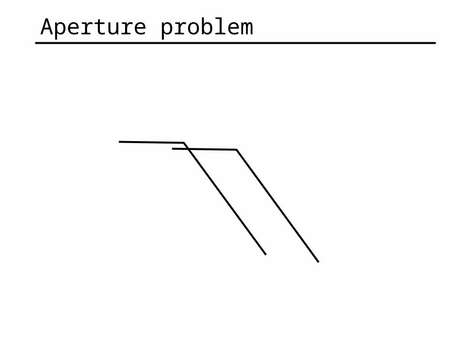
Aperture problem

Aperture problem

Solving the aperture problemBasic idea: assume motion field is smooth

Horn & Schunk: add smoothness term

Lukas & Kanade: assume locally constant motion• pretend the pixel’s neighbors have the same (u,v)

– If we use a 5x5 window, that gives us 25 equations per pixel!

• works better in practice than Horn & Schunk

Many other methods exist. Here’s an overview:• Barron, J.L., Fleet, D.J., and Beauchemin, S, Performance of optical flow

techniques, International Journal of Computer Vision, 12(1):43-77, 1994.• http://www.cs.washington.edu/education/courses/576/03sp/readings/barron92performance.pdf

Lukas-Kanade flowHow to get more equations for a pixel?

• Basic idea: impose additional constraints– most common is to assume that the flow field is smooth locally– one method: pretend the pixel’s neighbors have the same (u,v)

» If we use a 5x5 window, that gives us 25 equations per pixel!

RGB versionHow to get more equations for a pixel?

• Basic idea: impose additional constraints– most common is to assume that the flow field is smooth locally– one method: pretend the pixel’s neighbors have the same (u,v)

» If we use a 5x5 window, that gives us 25*3 equations per pixel!

Lukas-Kanade flowProb: we have more equations than unknowns

• The summations are over all pixels in the K x K window• This technique was first proposed by Lukas & Kanade (1981)

– described in Trucco & Verri reading

Solution: solve least squares problem• minimum least squares solution given by solution (in d) of:

Conditions for solvability

• Optimal (u, v) satisfies Lucas-Kanade equation

When is This Solvable?• ATA should be invertible • ATA should not be too small due to noise

– eigenvalues 1 and 2 of ATA should not be too small• ATA should be well-conditioned

– 1/ 2 should not be too large (1 = larger eigenvalue)

Eigenvectors of ATA

Suppose (x,y) is on an edge. What is ATA? derive on board

• gradients along edge all point the same direction• gradients away from edge have small magnitude

• is an eigenvector with eigenvalue• What’s the other eigenvector of ATA?

– let N be perpendicular to

– N is the second eigenvector with eigenvalue 0

The eigenvectors of ATA relate to edge direction and magnitude

Edge

– large gradients, all the same

– large1, small 2

Low texture region

– gradients have small magnitude

– small1, small 2

High textured region

– gradients are different, large magnitudes

– large1, large 2

ObservationThis is a two image problem BUT

• Can measure sensitivity by just looking at one of the images!

• This tells us which pixels are easy to track, which are hard– very useful later on when we do feature tracking...

Errors in Lukas-KanadeWhat are the potential causes of errors in this procedure?

• Suppose ATA is easily invertible• Suppose there is not much noise in the image

When our assumptions are violated• Brightness constancy is not satisfied• The motion is not small• A point does not move like its neighbors

– window size is too large– what is the ideal window size?

• Can solve using Newton’s method– Also known as Newton-Raphson method

– Today’s reading (first four pages)» http://www.ulib.org/webRoot/Books/Numerical_Recipes/bookcpdf/c9-4.pdf

• Lukas-Kanade method does one iteration of Newton’s method– Better results are obtained via more iterations

Improving accuracyRecall our small motion assumption

This is not exact• To do better, we need to add higher order terms back in:

This is a polynomial root finding problem

1D caseon board

Iterative RefinementIterative Lukas-Kanade Algorithm

1. Estimate velocity at each pixel by solving Lucas-Kanade equations

2. Warp H towards I using the estimated flow field- use image warping techniques

3. Repeat until convergence

Revisiting the small motion assumption

Is this motion small enough?• Probably not—it’s much larger than one pixel (2nd order terms dominate)

• How might we solve this problem?

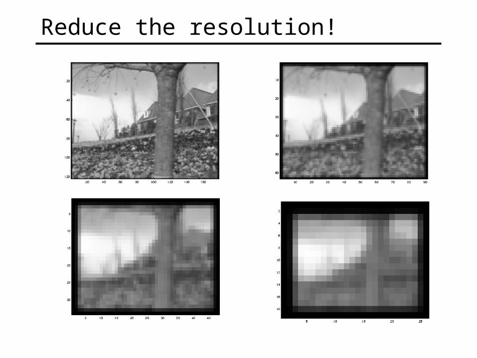
Reduce the resolution!

image Iimage H

Gaussian pyramid of image H Gaussian pyramid of image I

image Iimage H u=10 pixels

u=5 pixels

u=2.5 pixels

u=1.25 pixels

Coarse-to-fine optical flow estimation

image Iimage J

Gaussian pyramid of image H Gaussian pyramid of image I

image Iimage H

Coarse-to-fine optical flow estimation

run iterative L-K

run iterative L-K

warp & upsample

.

.

.

Optical flow result

Dewey morph

Robust methodsL-K minimizes a sum-of-squares error metric

• least squares techniques overly sensitive to outliers

quadratic truncated quadratic lorentzian

Error metrics

Robust optical flowRobust Horn & Schunk

Robust Lukas & Kanade

first image quadratic flow lorentzian flow detected outliers

Reference• Black, M. J. and Anandan, P., A framework for the robust estimation of optical flow, Fourth

International Conf. on Computer Vision (ICCV), 1993, pp. 231-236 http://www.cs.washington.edu/education/courses/576/03sp/readings/black93.pdf

Motion trackingSuppose we have more than two images

• How to track a point through all of the images?

Feature Tracking• Choose only the points (“features”) that are easily tracked• How to find these features?

– In principle, we could estimate motion between each pair of consecutive frames

– Given point in first frame, follow arrows to trace out it’s path– Problem: DRIFT

» small errors will tend to grow and grow over time—the point will drift way off course

– windows where has two large eigenvalues

• Called the Harris Corner Detector

Feature Detection

Tracking featuresFeature tracking

• Compute optical flow for that feature for each consecutive H, I

When will this go wrong?• Occlusions—feature may disappear

– need mechanism for deleting, adding new features

• Changes in shape, orientation– allow the feature to deform

• Changes in color• Large motions

– will pyramid techniques work for feature tracking?

Handling large motionsL-K requires small motion

• If the motion is much more than a pixel, use discrete search instead

• Given feature window W in H, find best matching window in I

• Minimize sum squared difference (SSD) of pixels in window

• Solve by doing a search over a specified range of (u,v) values– this (u,v) range defines the search window

Tracking Over Many Frames

Feature tracking with m frames1. Select features in first frame

2. Given feature in frame i, compute position in i+1

3. Select more features if needed

4. i = i + 1

5. If i < m, go to step 2

Issues• Discrete search vs. Lucas Kanade?

– depends on expected magnitude of motion– discrete search is more flexible

• Compare feature in frame i to i+1 or frame 1 to i+1?– affects tendency to drift..

• How big should search window be?– too small: lost features. Too large: slow

Incorporating DynamicsIdea

• Can get better performance if we know something about the way points move

• Most approaches assume constant velocity

or constant acceleration

• Use above to predict position in next frame, initialize search

Feature tracking demo

http://www.toulouse.ca/?/CamTracker/?/CamTracker/FeatureTracking.html

MPEG—application of feature tracking• http://www.pixeltools.com/pixweb2.html

Oxford video

Image alignment

Goal: estimate single (u,v) translation for entire image• Easier subcase: solvable by pyramid-based Lukas-Kanade