Annex A: Examples on estimation of uncertainty in

airflow measurement

Introduction

A.2 Example one — test facility

A.2. I Definition of the measurement process

This annex contains three examplesof fluid flowmeasurementuncertaintyanalysis. The first dealswith airflow measurementfor an entirefacility (withseveralteststands)overa longperiod. It alsoappliesto a singletestwith a singleset of instruments.Thesecondexampledemonstrateshow comparativede-velopmenttests can reducethe uncertaintyof thefirst example.The third exampleillustratesa liquidflow measurement.

A.1 General

Airflow measurementsin gasturbineenginesystemsare generally made with one of three types offlowmeters:venturis,nozzlesandorifices. Selectionofthe specific type of flowmeter to use for a givenapplication is contingent upon a tradeoff betweenmeasurementaccuracyrequirements,allowablepres-suredropandfabricationcomplexityandcost.

Flowmetersmaybefurtherclassifiedinto two catego-ries: subsonicflow andcritical flow. With a criticalflowmeter, in which sonic velocity is maintainedattheflowmeterthroat,massflowrateis afunctiononlyof the upstream gas properties.With a subsonicflowmeter, where the throat Mach number is lessthan sonic, mass flowrate is a function of bothupstreamanddownstreamgasproperties.

Equations for the ideal mass flowrate through noz-zles, venturies and orifices are derived from thecontinuityequation:

W = paV

In usingthe continuity equationas a basis for idealflow equationderivations, it is normal practice toassumeconservationof massand energy and one-dimensional isentropic flow. Expressionsfor idealflow will not yield actualflow sinceactualconditionsalwaysdeviatefrom ideal.An empirically determinedcorrectionfactor,the dischargecoefficient (C) is usedto adjustidealto actualflow:

C Wac~/Wjdea~

Whatisthe airflow measurementcapabilityof a givenindustrialor governmenttest facility? This questionmight relateto a guaranteein a productspecificationora researchcontract.Notethat this questionimpliesthat many test stands,sets of instrumentationandcalibrationsover a long period of time should beconsidered.

Thesamegeneraluncertaintymodel is appliedin thesecondexampleto asinglestandprocess,thecompar-ativetest.

Theseexampleswill provide,stepby step,the entireprocessof calculatingthe uncertaintyof the airflowparameter.Thefirst stepis to understandthedefinedmeasurementprocessandthen identify thesourceofevery possibleerror.For eachmeasurement,calibra-tion errorswill be discussedfirst, then dataacquisi-tion errors,datareductionerrors,andfinally, propa-gationof theseerrorsto thecalculatedparameter.

Figure 14 depictsacritical venturi flowmeterinstalledin the inlet ducting upstreamof a turbine engineundertestfor this example.

When a venturi flowmeter is operatedat criticalpressure ratios, i.e., (P2/P1) is a minimum, theflowrate through the venturi is a function of theupstreamconditionsonly andmay becalculatedfrom

d2 PW = ~~CFa(P•~

A.2.2 Measurement error sources

(41)

(39) Eachof the variablesin equation41 mustbecarefullyconsideredto determine how and to what extenterrorsin the determinationof the variableaffect thecalculatedparameter.A relativelylarge errorin somewill affectthe final answerverylittle, whereassmallerrors in others havea large effect. Particularcareshouldbetakento identify measurementsthat influ-encethe fluid flow parametersin morethanoneway.

In equation(41), upstreampressureandtemperature(P1andT1) areof primaryconcern.Error sourcesforeachof thesemeasurementsare: (1) calibration, (2)

(40) dataacquisitionand(3) datareduction.

27

026O~

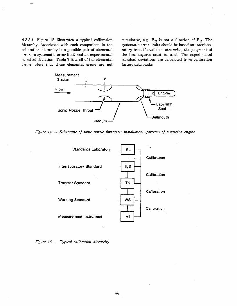
A.2.2. 1 Figure 15 illustrates a typical calibrationhierarchy. Associatedwith each comparisonin thecalibration hierarchyis a possiblepair of elementalerrors,a systematicerror limit andan experimentalstandarddeviation.Table 7 lists all of theelementalerrors. Note that these elemental errors are not

cumulative,e.g., B21 is not a function of B11. Thesystematicerror limits shouldbe basedon interlabo-ratory testsif available,otherwise,the judgment ofthe best expertsmust be used. The experimentalstandarddeviations are calculatedfrom calibrationhistorydatabanks.

Figure 14 — Schematicof sonic nozzleflowmeter installation upstreamof a turbine engine

Standards Laboratory

1MeasurementStation

Flow

Sonic Nozzle Throat

Plenum

LabyrinthSeal

Belimouth

Calibration

Calibration

Calibration

Interlaboratory Standard

Transfer Standard

Working Standard

Measurement Instrument

Figure 15 — Typical calibration hierarchy

Calibration

28

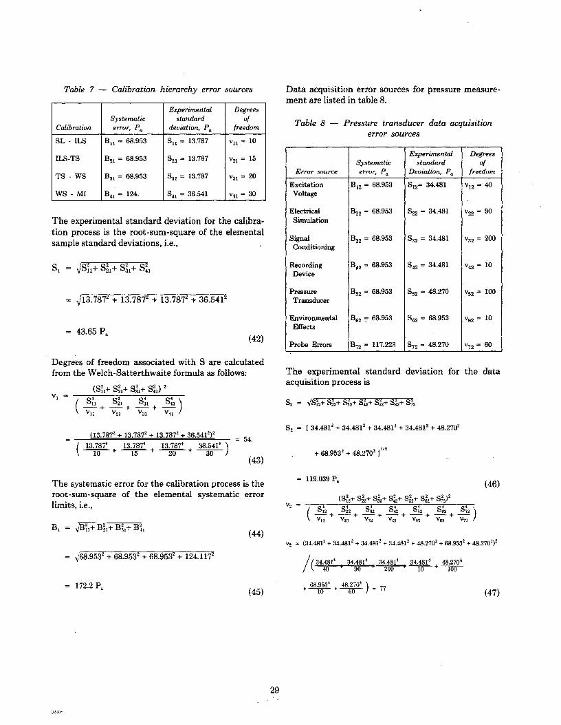
Table 7 — Calibration hierarchy error sources Dataacquisitionerror sourcesfor pressuremeasure-

The experimental standardacquisitionprocessis

S2

= ~ S~2

÷S~2

÷S~2

+S~2

+S~2

+S~2

68.953~ 48.270~+ 10 ÷ 60 )~77

CalibrationSystematicerror, P

0

Experimentalstandard

deviation, P0

Degreesof

freedom

SL - ILS

ILS-TS

TS - WS

WS - MI

B11

6&953

B21

= 68.953

B31

68.953

B41

124.

S11

13.787

S21

13.787

S31

13.787

S41

36.541

v11

10

v21

= 15

v31

20

v41

= 30

mentarelistedin table8.

Table 8 — Pressuretransducerdata acquisitionerror sources

Error sourceSystematicerror, P

0

Experimentalstandard

Deviation, P0

Degreesof

freedom

ExcitationVoltage

B12

= 68.953 S12

= 34.481 v12

= 40

ElectricalSimulation

B92

68.953 S22

= 34.481 v22

90

SignalConditioning

B32

68.953 S32

= 34.481 v32

= 200

RecordingDevice

B42

= 68.953 S42

= 34.481 v~= 10

PressureTransducer

B52

68.953 S52

= 48.270 v52

100

EnvironmentalEffects

B62

= 68.953 ~62 68.953 v62

= 10

Probe Errors B72

117.223 S72

= 48.270 V72

= 60

The experimentalstandarddeviationfor the calibra-tion processis the root-sum-squareof the elementalsamplestandarddeviations,i.e.,

S1 = \/Sll+ S21+ S11+ S41

= ~Ji~?~872+ 13.7872 + 13.7872+ 36.5412

43.65Pa (42)

Degreesof freedomassociatedwith S arecalculatedfrom theWelch-Satterthwaiteformulaasfollows:

(S~1÷S~1

÷S~1

÷S~1

)2vl= / ~4 Q

4Q

4Q

4

I ~‘1i ~‘21 ~31 ~~4j—+ —+ —÷ —

V11

V21

V31

V41

— (13.787~+ 13.787~+ 13.7872+ 36.541~)~ =

— ( 13.787’ 13.787’ 13.787’ 36.541’10 ÷ 15 + 20 ÷ 30

(43)

The systematicerrorfor the calibrationprocessis theroot-sum-squareof the elementalsystematicerrorlimits, i.e.,

B1 = ~1B~÷B~1÷B~~1 (44)

(45)

deviation for the data

S2

[34.481~~ 34.4812+ 34.4812+ 34.4812+ 48.2702

÷68.9532+ 48.270211/2

= 119.039P0

(46)

(S~3

+S~÷S~2

÷S~÷S2

÷S~÷5~)2= / S~ S~ S

32S

42S

52S

02S

32

“12 + “22 ÷ “32 “42 + ‘p52 ÷ ~/52 + V~

(34.481~÷34.4812÷34.4812÷34.4812+ 48270~+ 689532 + 48.2702)2

// 34.481’ 34.481’ 34.481’ 34.481~ 48.270’/ t, 40 + 90 ÷ 200 ÷ 10 ÷ 100

(47)

= V68.953’ ÷68.953’÷68.953’÷124.117’

172.2 P.

29

0244),

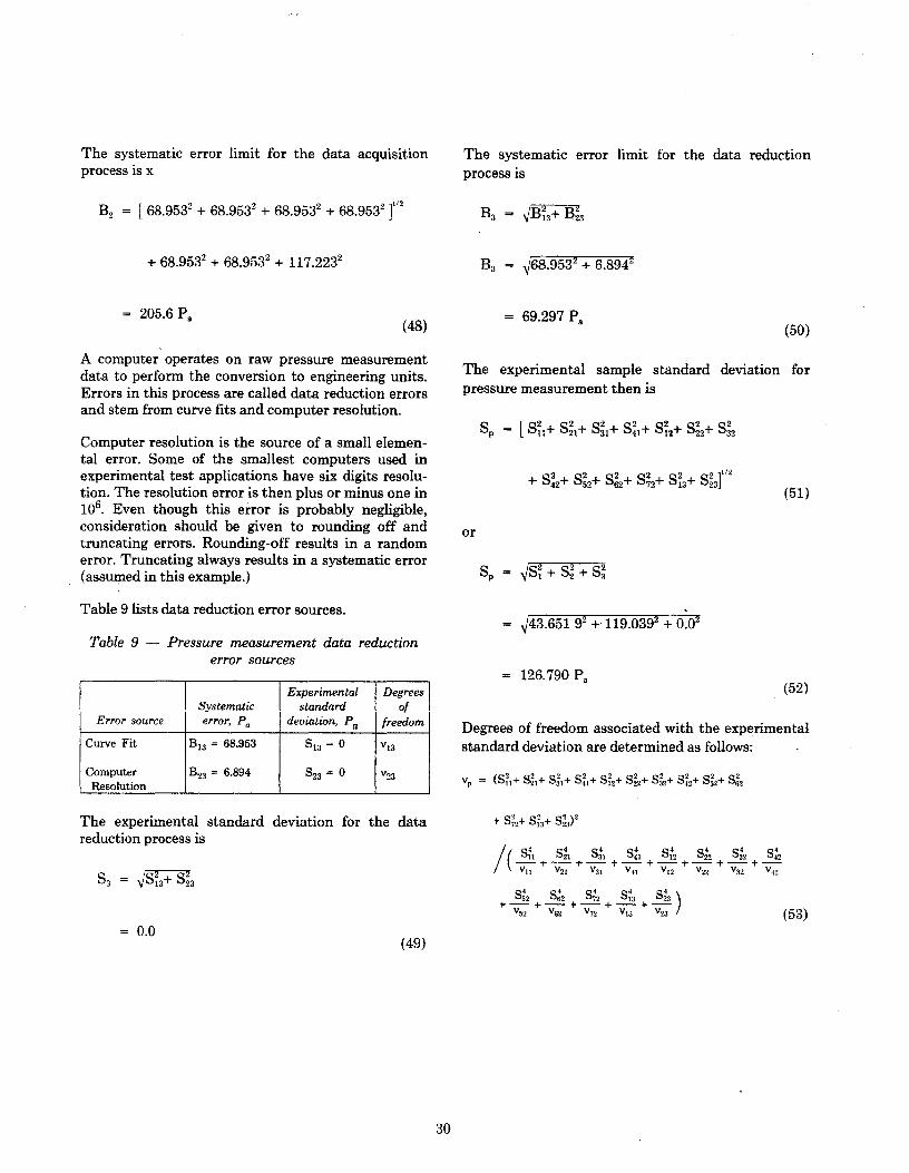
The systematicerror limit for the dataacquisitionprocessis x

B2 = [68.9532 + 68.9532 + 68.9532 + 68.9532}l/2

+ 68.9532 + 68.9532 + 117.2232

The systematicerror limit for the data reductionprocessis

B3 = ~jB~3÷B23

B3 = ~/68.9532 + 6.8942

= 205.6~a(48)

or

= 69.297P5

S9 = ~JS~+ S~+ S~

(50)

(51)

Table9 listsdatareductionerrorsources.

Table 9 — Pressuremeasurementdata reductionerror sources

Error source—

Systematicerror, P

0

Experimental Degreesstandard of

deviation, ~a LfreedomCurve Fit

ComputerResolution

B13

= 68.953

B.,3

6.894

S13

= 0

S23

= 0

v~3

v23

The experimentalstandarddeviation for the datareductionprocessis

S3 = .,JS~3+S~3

= 0.0(49)

= V43.65192 ~ 119.0392 + 0.02

= 126.790Pa(52)

Degreesof freedomassociatedwith the experimentalstandarddeviationaredeterminedasfollows:

v~= (S~1

+S~1

÷S~1

+S~1

÷S~÷S~2~S3~+S42

+ 5~,÷S62

+ S~2

+S~,÷S~3)’

/ S~~l S~ ~ S~1

S~2

~ S~2 542

/ (__+ +—÷—÷_÷ +—~ V42

+—V11

V21

V31

V.51

V12

V22

V3~

S2

S2

S~2

S~3 S~3~

+— ÷— ÷— ÷— +V

52V

62V

72V

13V

23I (53)

A computeroperateson raw pressuremeasurementdata to perform the conversionto engineeringunits.Errorsin this processare calleddatareductionerrorsandstemfromcurvefits andcomputerresolution.

Computerresolutionis the sourceof a small elemen-tal error. Some of the smallestcomputersused inexperimentaltestapplicationshavesix digits resolu-tion. Theresolutionerroris thenplus orminusonein106. Even though this error is probably negligible,considerationshould be given to rounding off andtruncatingerrors. Rounding-offresults in a randomerror.Truncatingalwaysresultsin asystematicerror(assumedin this example.)

The experimental sample standarddeviation forpressuremeasurementthenis

= [S~1+S~1+S~1÷S~1÷S~2÷S~2÷S~2

+ S~2~S~÷S~2÷S~2+S~÷52]h/2

30

A.2.2.2 The calibration hierarchy for temperaturemeasurementsis similar to that forpressuremeasure-ments.Figure 16 depictsa typical temperaturemea-surementhierarchy. As in the pressurecalibrationhierarchy,eachcomparisonin the temperaturecalib-ration hierarchy may produceelementalsystematic

andrandomerrors.Table 10 lists temperaturecalib-ration hierarchyelementalerrors.

Table 10 — Temperaturecalibration hierarchyele-mental errors

CalibrationSystematicerror, K

Experimentalstandard

deviation,K

Degreesof

freedom

SL - ILS

ILS-TS

TS - WS

WS - MI

B11

0.056

B21

= 0.278

B31

= 0.333

B41

= 0.378

0.002

~21 = 0.028

~31 = 0.028

S41

= 0.039

2

V21

= 10

= 15

v41

30

The calibrationhierarchyexperimentalstandardde-viationis calculatedas

SI = VS’~2±S~1+S~1+S~

Degreesof freedomassociatedwith S1are

(S~1÷S~1÷S~1-t-S~1)2V

1= ~

4

(!!V11

+ V21

V31

V41

/

— (0.002~÷0.0282÷0.0282+ 0.0392)2

— 1 0.002’ 0.028~ 0.028k 0.039~2 ÷ 10 ÷ 15 + 30

Thecalibrationhierarchysystematicerrorlimit is

or

— (S~-i-S~+S~)2

VP_f S~ S~ S~

‘~-~-÷ —;;;;-+ -~--

— (43.65192 + 119.0392+ 0.02)2— 1 43.65192 119.0392 O.O~

Is\ 54. ÷ 77 +—~-—

96 thereforet9~= 2.(54)

The systematicerror limit for the pressuremeasure-ment is

B~= [B~1÷B~1÷B~1÷B~1÷B~2÷B~+B~2

+ B~2+B~2+B~2÷B~9÷B~3÷B~3]L~2

or

B9 = ~‘B~+ B~+ B~

B9 = y172.2462+ 205.593~+ 69.2972

= 277.018Pa (56)

Uncertaintyfor thepressuremeasurementis

U~9= (B9 + t95

S9),U9~= ~JB~+ (t~S9)2

U~= (277.018+ 2 x 126.790)

= 530.598P U95 = 375.6PV a (57)

= V0.0022

+ 0.0282+ o.o2S2+ 0.0392

= 0.056°K.

= 53 > 30, thereforet95

= 2.

(58)

(59)

(60)

(61)

B1 = ,5/B~1÷B~1÷B~1+~2

= ~j0.0562+ 0.2782+ 03332 + 0.3782

= 0.578 ~}(

31

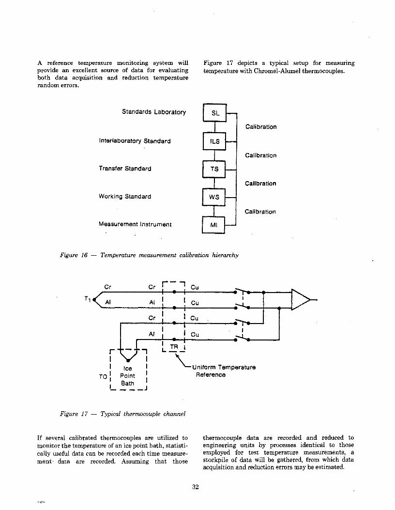
A reference temperature monitoring system willprovide an excellent source of data for evaluatingboth data acquisition and reduction temperaturerandomerrors.

Figure 17 depicts a typical setup for measuringtemperaturewith Chromel-Alumelthermocouples.

Standards Laboratory

Interlaboratory Standard

Transfer Standard

Working Standard

Measurement Instrument

Figure 16 — Temperaturemeasurementcalibration hierarchy

Ii

If several calibrated thermocouplesare utilized tomonitorthetemperatureof an icepointbath,statisti-cally useful datacanbe recordedeachtime measure-ment data are recorded. Assuming that those

thermocoupledata are recorded and reduced toengineering units by processesidentical to thoseemployed for test temperaturemeasurements,astockpile of data will be gathered,from which dataacquisitionandreductionerrorsmaybeestimated.

Calibration

Calibration

Calibration

Calibration

Cr Cu

r -II I

Ice

TO PointBath

L___i

L.i~J

Uniform TemperatureReference

Figure 17 — Typical thermocouplechannel

32

7) Computerresolutionerror

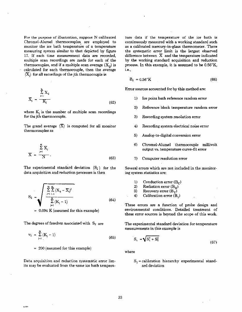
For the purpose of illustration, supposeN calibrated ture data if the temperature of the ice bath isChromel-Alumel thermocouplesare employed to continuouslymeasuredwith aworking standardsuchmonitor the ice bath temperatureof a temperature as a calibratedmercury-in-glassthermometer.Theremeasuringsystemsimilar to that depictedby figure the systematicerror limit is the largest observed17. If each time measurementdata are recorded, differencebetweenX andthetemperatureindicatedmultiple scan recordingsare made for each of the by the working standardacquisitionand reductionthermocouples,andif a multiple scanaverage(X1~)iscalculatedfor each thermocouple,then the average

process.In this example,it is assumedto be O.56°K,i.e.,

(Xi) forall recordingsof thejth thermocoupleis

. B~= 0.56°K (66)

Errorsourcesaccountedfor by this methodare:

x = K1 (62)1) Ice pointbathreferencerandomerror

2) Referenceblock temperaturerandomerrorwhere K- is the numberof multiple scanrecordingsfor the thermocouple.

.

3) Recordingsystemresolutionerror

The grandaverage (X) is computedfor all monitor 4) Recordingsystemelectricalnoiseerrorthermocouplesas

5) Analog-to-digitalconversionerror

N —

~ X3

6) Chromel-Alumel thermocouple millivoltoutputvs. temperaturecurve-fit error

x= N (63)

The experimentalstandarddeviation (Si) for the Severalerrorswhicharenot includedin themonitor-dataacquisitionandreductionprocessesis then ing systemstatisticsare:

S-=(64)

-

= 0.094K (assumedfor this example)

These errors are a function of probe design andenvironmental conditions. Detailed treatment oftheseerror sourcesis beyondthe scopeof this work.

Thedegreesof freedomassociatedwith S~are The experimentalstandarddeviationfor temperature

Nmeasurementsin this exampleis

v~= ~(K1-1) (65)S1 =S~S1+S~ (67)

= 200 (assumedfor this example)where

Dataacquisitionand reductionsystematicerror urn- S1= calibration hierarchy experimentalstand-its maybe evaluatedfrom the sameicebathtempera- arddeviation

E~(X8_X1)2j~1i—i

~(K3-1)j~1

33

0/Gil,

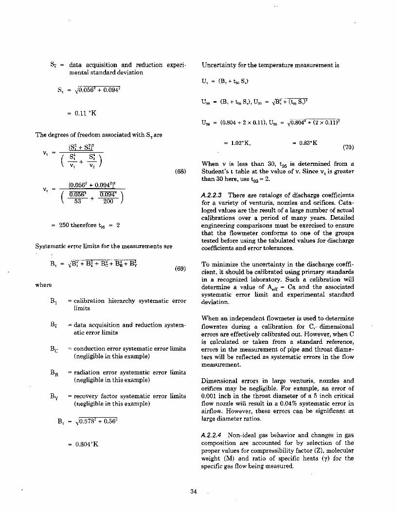
S7 = 310.0562+ 0.0942

The degreesof freedomassociatedwith S~are

U~= (0.804 + 2 x 0.11),U95 = + (2 x 0.11)2

When v is less than 30, t95 is determinedfrom a(68) Student’st tableat thevalueof v. Sincev~is greater

than 30 here,uset95= 2.

A.2.2.3 There arecatalogsof dischargecoefficientsfor a variety of venturis,nozzlesandorifices. Cata-logedvaluesare theresult of a largenumberof actualcalibrationsover a period of many years. Detailedengineeringcomparisonsmustbe exercisedto ensurethat the flowmeter conforms to one of the groupstestedbeforeusingthetabulatedvaluesfor dischargecoefficientsanderrortolerances.

where

B, =

B1 = calibration hierarchy systematicerrorlimits

B1 = dataacquisitionandreductionsystem-atic errorlimits

Bc = conductionerrorsystematicerrorlimits(negligiblein this example)

BR = radiation error systematicerror limits(negligible in this example)

B~ = recovery factor systematicerror limits(negligible in this example)

B, = V0.5782+ 0.562

69 To minimize the uncertaintyin the dischargecoeffi-cient, it shouldbecalibratedusingprimary standards

in a recognizedlaboratory. Such a calibration willdeterminea value of Aeff = Ca and the associatedsystematicerror limit and experimental standarddeviation.

Whenan independentflowmeter is usedto determineflowrates during a calibration for C,~dimensionalerrorsareeffectivelycalibratedout. However,whenCis calculatedor taken from a standardreference,errors in themeasurementof pipe andthroatdiame-terswill be reflectedassystematicerrorsin the flowmeasurement.

Dimensional errors in large venturis, nozzles andorifices may be negligible. For example,an error0.001 inch in the throat diameterof a 5 inch criticalflow nozzlewill result in a 0.04% systematicerror inairflow. However, theseerrors can be significant atlargediameterratios.

A.2.2.4 Non-idealgas behaviorand changesin gascomposition are accountedfor by selectionof thepropervaluesfor compressibilityfactor (Z), molecularweight (M) and ratio of specific heats (y) for thespecific gas flow beingmeasured.

S1 = data acquisition and reduction experi-mentalstandarddeviation

= 0.11 ~}(

Uncertaintyfor thetemperaturemeasurementis

U, (B,÷t~5S,)

= (B, 4- t95 S,), U95 = + (t95

S,)2

= 1.02°K, 0.83°K— (S~÷S~)2

V7

— / ~4 ~4

I ‘-ii ~-‘2—+ —

‘ V1

V2

— (0.0562+ 0.0942)2— I 0.056k ØQ944

53 + 200

= 250 thereforet95 = 2

Systematicerrorlimits for themeasurementsare

(70)

= 0.804°K

34

When values of y andZ are evaluatedat the properpressureand temperatureconditions, airflow errorsresulting from errors in ‘y andZ will be negligible.

For the specific case of airflow measurement,themain factor contributingto variationof compositionis the moisturecontentof theair. Though small, theeffectof achangein air densitydue to watervaporonairflow measurementshouldbe evaluatedin everymeasurementprocess.

A.2.2.5 The thermal expansion correction factor(Fa) corrects for changesin throat areacausedbychangesin flowmetertemperature.

For steels,a 17~Kflowmeter temperaturedifference,betweenthetimeof atestandthetimeof calibration,will introducean airflow error of 0.06%if no correc-tion is made. If flowmeter skin temperature isdeterminedto within 3°Kandthe correctionfactorapplied,the resultingerrorin airflow will be negligi-ble.

A.2.3 Propagation of error to airflow

For an exampleof propagationof errors in airflowmeasurementusinga critical-flow venturi,consideraventuri having a throat diameterof 0.554 meters

operatingwith dry air at an upstreamtotal pressureof 88 126~

aand an upstreamtotal temperatureof2659°K.

Equation(71) is the flow equationto be analyzed:

icd2* P1W = —~---CF5p7r~-

____ y+1( 2 ~7—1 (‘ygM

(p— \y+11 ~ZR (71)

Assume,for this example,that the theoreticaldis-chargecoefficient (C) has been determinedto be0.995. Further assumethat the thermal expansioncorrectionfactor (Fa) andthe compressibilityfactor(Z) are equal to 1.0. Table 11 lists nominal values,systematicerror limits, samplestandarddeviationsand degreesof freedomfor eacherror sourcein theaboveequation.(To illustrate the uncertaintymeth-odology, we will assumea samplestandarddeviationof 0.0005 in additionto a systematicerror of 0.003.)

Note that, in table II, airflow errors resultingfromerrors in Fa* Z, k, g, M and R are considerednegligible.

Table 11 — Airflow measurementerror sources

Errorsource

V

UnitsNominal

value

Systematicerrorlimit

Experime~ta1standarddeviation

Degreesof

freedom,V

UncertaintyU~

P1

P5

88 126 217.02 126.79 96 530.60

T1

K 265.9 0.8 0.11 250 1.02

d m 0.554 2.54X105

2.54X10~ 100 7.62X105

C 0.995 0.003 O000 5 — 0.003

~a 1.0 — — — —

z 1.0 — — — —

y 1.401 — — — —

g — — — —

M kg/kg-mole 28.95 — — — —

H J/K-kg-mole 8.3 14 — — — —

35

0260,

Fromequation(71), airflow iscalculatedas

w = 3.142 (0554)2x 0.995 x 1.0

= 52.39 kg/sec.

Taylor’s seriesexpansionof equation(71) with theassumptions indicatedyields equations(72) and(73)from which the flow measurementexperimental

standarddeviation and systematicerror limits arecalculated.

s~= w s,l (~)2(~L)2(s)2(~5)2

11 126.790 \2 ( —0.11= 52.39L ~. 88 126 1 + k 2 x 265.9 1

2 2 1/21 0.0005 \ 1 2 x 0.000025~k 995 1 -‘-‘s 0.554

which resultsin an overall degreesof freedom>30,and,therefore,avalueoft95of 2.0.

Total airflow uncertaintyis then,

U99 = (B,~+ t95 Sw), U95 = 31B~+ (t95

S~)2

U~= [0.2416 + 2 x 0.0787]

= 0.40 kg/sec

= 0.8%

= 52.39 ~(0.001 4)2 + (—0.000 2)2 + (~~05o3)2~O.oo0Ø~j2

= 0.0787 kg/sec

B~= w~(~)+(4~)÷(4~)÷(4t)

11 277.02 \2 f —0.804 \2 f 0.003B,, = o239Lk88126 ) ~ 531.8 1 ~

1 0.00005~\ 0.554 1 J

= 52.39 ~/(0.0031)2+ (—0.001 5)2 + (0.003Q)2 + (0.00009)2

0.241 6 kg/seg

By using the Welch-Satterthwaiteformula, the de-grees of freedom for the combined experimentalstandarddeviationis determinedfrom

A.3 Example two — comparative test

A.3. 1 Definition of themeasurementprocess

The objective of a comparativetest is to determinewith the smallestmeasurementuncertaintythe neteffect of adesignchange,suchasanewpart.Thefirsttest is performed with the standard or baseline

(73) configuration. A secondtest, identical to the firstexcept that the design changeis substitutedin thebaseline configuration, is then carried out. Thedifference betweenthe measurementresults of thetwo tests is an indication of the effect of the designchange.

FI~W ‘ClawL~~S

91j ÷~~-ST

1) +

vV* = 4 4

( aw ~ ‘~ ÷ I a’~v ÷‘~~p•;- Pu ~ ~ TjJ

2 229W \ I ow

—a—Sd; ÷~-~--sc4 4

OW \ ÷~ ~c

Vd vC

As long as we only consider the difference or neteffect betweenthe two tests,all the fixed, constant,systematicerrors will cancelout. The measurementuncertainty is composedof random errorsonly.

For example, assumewe are testing the effect on thegasfiowof a centrifugalcompressorfrom achangetothe inlet inducer. At constant inlet and discharge

4(

2 \0.4012.4012.401 ) 1 1.401x 28.95 \ 88 1268314 )x~___

2 /5

T )2 + ( 2Sd 2 2 12

~5

T1

~4 I 2S4 \4 ( __~c_’i4(~)+( ~ c~“P

Vp1

VT, Vd ‘1

C

(74)

(72)

U95 = 0.29 kg/sec

= 0.55%(75)

36

conditions,andconstantrotationalspeed,will thegasflow increase?If we testthe compressorwith the oldandnew inducersandtakethe differencein measuredairflow as our defined measurementprocess, weobtain the smallestuncertainty.All the systematicerrors cancel.Note that, although the comparativetestprovidesanaccurateneteffect,the absolutevalue(gasfiowwith the newinducer)is notdeterminedo~ifcalculated,as in exampleone,it will beinflatedby thesystematicerrors.Also, the small uncertaintyof thecomparative test can be significantly reduced byrepeatingit severaltimes.

A.3.2 Measurement error sources

(see equation (65))

A.3.2.3 The test result is the difference in flowbetweentwo tests.

= WI — W2

All errorsresult from randomerrors in dataacquisi-tion and datareduction.Systematicerrors areeffec-tively zero.Randomerrorvaluesareidenticalto thosein exampleone,exceptthatcalibrationrandomerrorsbecomesystematicerrorsand,hence,effectivelyzero.

= (BA,,, + 2SAW)

= (0 + 2SAW)

= 31(BAW)2÷(2SAW)2

= 31o2 + (2SA~)2

A.3.2. 1 Comparativetests shall use the sametestfacility andinstrumentationfor eachtest.All calibra-tion errorsare systematicandcancelout in takingthedifferencebetweenthetestresults.

B1 = 0

S1 = 0, Sc = 0

SP = S2

= 2SA~ =2SAW

UAW~ = 2S~\/~ U~,5= 2S~1J~

S ± 52 39 { ( 119.037 \2 1 —0.094 \2= — 88 126 ) ÷~2x265.9 )

/ 0.0005 )2( 0.00005 \,11~’2 V

÷~ 0.995 0.554 J J

S,, = 0.076 2 kg/sec SAW = 0.107 8 kg/sec

UA,,~=0.2155 kg/sec

= 0.41%

= 0.2155 kg/sec

= 0.41%

= 119.039 Pa(see equation (47)) (seeequation(75))

VP = V9

= 77

St = S1

= 0.094°K

(see equation (48))

(seeequation (64))

37

A.3.2A Note that the differencesshownin table12are entirely due to differencesin the measurementprocessdefinitions.Thesamefluid flow measurementsystemmight be usedin bothexamples.The compar-ative testhas the smallestmeasurementuncertainty,but this uncertainty value does not apply to themeasurementof absolutelevel of fluid flow, only tothedifference.

V, V1

= 200

SAW 31S~1÷(—i)2S~2=s,,31~

and

A.3.2.2

0260,

1. 2,3. m Observationpoints

b1,b2,b3,. . b~ Breadth(metres)of segmentassociatedwith theobservationpoint

V d1,d2,d3,. . d~.g Depthof water(metres)at theobservationpoint

Dashedlines Boundaryof segments:oneheavilyoutlined

If x andy are respectivelyhorizontal and vertical coordinatesof all the points in the cross-section,and A is its total area, then the precisemathematicalexpressionfor ~ the true

volumetricflowrate(discharge)acrossthearea,canbewritten as

Figure 18 — Definition sketchof velocity-areamethod of dischargemeasurement(midsectionmethod)

L~,4 1)5

lnrt!aIpoint

T~T~

Explanation

38