EUR 24475 EN - 2010

Estimation of the measurement uncertainty of ambient air pollution datasets using geostatistical analysis

Michel Gerboles* and Hannes I. Reuter + *Joint Research Centre, Institute for Environment an d Sustainability, Ispra, Italy+Gisxperts gbr, Dessau, Germany

The mission of the JRC-IES is to provide scientific-technical support to the European Union’s policies for the protection and sustainable development of the European and global environment. European Commission Joint Research Centre Institute for Environment and Sustainability Contact information Address: Michel Gerboles, Via E. Fermi 2749, I - 21027 Ispra (VA) E-mail: michel.gerboles@jrc.ec.europa.eu Tel.: +39 0332 785652 Fax: +39 0332 789931 http://ies.jrc.ec.europa.eu/ http://www.jrc.ec.europa.eu/ Legal Notice Neither the European Commission nor any person acting on behalf of the Commission is responsible for the use which might be made of this publication.

Europe Direct is a service to help you find answers to your questions about the European Union

Freephone number (*):

00 800 6 7 8 9 10 11

(*) Certain mobile telephone operators do not allow access to 00 800 numbers or these calls may be billed.

A great deal of additional information on the European Union is available on the Internet. It can be accessed through the Europa server http://europa.eu/ JRC 59441 EUR 24475 EN ISBN 978-92-79-16358-6 ISSN 1018-5593doi:10.2788/44902 Luxembourg: Publications Office of the European Union © European Union, 2010 Reproduction is authorised provided the source is acknowledged Printed in Italy

Abstract

We developed a methodology able to automatically estimate of measurement uncertainty in the air pollution data sets of AirBase. The figures produced with this method were consistent with expectations from laboratory and field estimation of uncertainty and with the Data Quality Objectives of European Air Quality Directives. The proposed method based on geostatistical analysis is not able to estimate directly the measurement uncertainty. It estimates the nugget effect from variogram modelling together with a micro-scale variability which must be minimized by accurate selection of the type of station. Based on the results obtained so far, it is likely that measurement uncertainty is best estimated using all background stations of whatever area type. So far the methodology has been used to estimate measurement uncertainty in datasets from 4 different countries independently. This work should be continued for the whole Europe or for background station without national borders. The method has been shown to be also useful to compare the spatial continuity of air pollution in different countries that seems to be influenced by the spatial distribution of the stations (e.g influenced by topography) of each country.

Moreover, the method may be used to quantify the trend of measurement uncertainty over long periods (decades) with the possibility to evidence improvement in the data quality of AirBase datasets.

The implemented outlier detection module would be of interest as the warning system when countries report their measurements to the European Environment Agency. The method could also provides a simple solution to investigate the assignment and accuracy of station classification in AirBase.

Acknowledgement The authors would like to express their gratitude to Valentin Foltescu, Project Manager, of the Air and Climate Change Programme of the European Environment Agency in Copenhagen – Denmark for reviewing this report.

Table of Contents Abstract ................................................................................................................................................................... 3

Introduction ............................................................................................................................................................ 5

Methodology ........................................................................................................................................................... 7

AirBase ................................................................................................................................................................ 7

Geostatistical method ......................................................................................................................................... 8

Development of a methodology for downloading geo-referenced air pollution data series of AirBase and

automatic estimation of the nugget variance of their variogram; ................................................................... 12

Estimation of the measurement uncertainty using the nugget variance ............................................................. 19

Trend over time of the measurement uncertainty indicated by the nugget effect ............................................. 24

Create a warning system for classification of monitoring stations ....................................................................... 27

Conclusions ........................................................................................................................................................... 33

Future study: ......................................................................................................................................................... 34

Appendix I: Developed R- Routines....................................................................................................................... 37

Appendix II: Developed Shell Script for Data import into the PostgresSQL Database ......................................... 37

5

Introduction

The European Commission has worked intensively on the implementation of a harmonized programme

for the monitoring of air pollutants including arsenic (As), cadmium (Cd), nickel (Ni), benzo(a)pyrene,

mercury (Hg), sulphur dioxide (SO2), nitrogen oxides (NO/NO2), ozone (O3), benzene, carbon

monoxide (CO), benzene and particulate matter (PM10/PM2.5) and lead (Pb) in ambient air. The

harmonization program relies on the adopted European Directives 2008/50/EC and 2004/107/EC [1,2].

These directives defines limit and target values for air pollution that should not be exceeded if harmful

effects on the population and the environment are to be avoided. Exceedances of these limits may have

legal consequences that trigger measures aiming at reducing the exceeded limit values. To avoid those

measurement artefacts triggering such measures, the Directives endeavour to improve the quality of

the measurements by defining stringent protocols for the sampling/analysis/calibration methods and

for the implementation of Quality Assurance/Quality Control programs (QA/QC). They also define

data quality objectives (DQOs) that represent the highest allowed relative expanded uncertainty of

measurements applied in the region of the Limit Values. The reference methods exhibiting the highest

metrological quality of the Directives have been standardized by the European Committee for

Standardization (CEN). These standards describe the methodology to be applied for the estimation of

the measurement uncertainty. This estimation of the uncertainty of measurements is a long and tedious

procedure that may require considerable experimental work. The European Directives allows that two

methods of uncertainty estimation are applied following the guidance provided in a CEN report [3]:

� one is based on the Guide to the Expression of Uncertainty in Measurement [4], generally called

the direct-approach or GUM method, in which the uncertainty of a measurement is described with

1 Directive 2004/107/EC of the European Parliament and of the Council of 15 December 2004 relating to arsenic, cadmium, mercury , nickel and polycyclic aromatic hydrocarbons in ambient air. Official Journal L 23, 26/01/2005. 2 Directive 2008/50/EC of the European Parliament and the Council of 21 May 2008 on Ambient Air Quality and Cleaner Air for Europe, Official Journal of the European Union L 152/1 of 11.6.2008 3 Air Quality—Approach to Uncertainty Estimation for Ambient Air Reference Measurement Methods (CR14377:2002E) 4 International Organisation for Standardisation, Guide to the expression of uncertainty in measurement, ISBN 92-67-10188-9, ISO, Geneva, 1995

6

a measurement model that includes several input quantities representing physical variables

influencing the measurement. The standard uncertainty of all input quantities must be separately

determined and are subsequently combined according to the law of propagation of errors to

estimate the uncertainty of the measurement;

� the second method is based on the determination of “Accuracy (trueness and precision) of

measurement methods and results” [5], the so called indirect approach, which is concerned

exclusively with the uncertainty of measurement methods. The model explaining the measurement

Y is based upon the sum of the overall mean, the laboratory bias and the random error. The

laboratory bias and random error components are, in quantitative terms, obtained by a

collaborative study consisting in an interlaboratory experiment run under reproducibility

conditions whose results are treated using the analysis of variance (ANOVA) method.

Nowadays, the methods of estimation of the uncertainty of measurements of ambient air pollution

made in Europe are well known. This estimation in carried out on a routine basis by the laboratories

reporting their measurements in AirBase, the database maintained by the European Environment

Agency (EEA).

From another perspective, it is possible to derive the uncertainty of spatially referenced measurements

from the nugget effect of variogram analysis. The nugget effect represents fluctuations of the

measurements on a very small scale (tending towards 0). It is often decomposed into the sum of micro-

scale variations of the measurand under study and of the measurement errors [6].

In this report, we discuss about the possibility to automatically derive the uncertainty of measurements

of ambient air pollutant using a new method based on geostatistical analysis of the spatially referenced

datasets present in AirBase, using semi-variogram analysis. This report presents the results of a

feasibility study in order to:

5 International Standards, 1994, Accuracy (trueness and precision) of measurement methods and results - Part 2: Basic method for the determination of repeatability and reproducibility of a standard measurement method, ISO 5725-2:1994, Geneva, Switzerland.

7

1. Develop a methodology for downloading geo-referenced air pollution data series of AirBase

and for the automatic estimation of the parameters of their spherical variogram;

2. Discuss the uncertainty of measurement evaluated using the estimated nugget variance

compared to the DQO for a chosen pollutant, PM10;

3. Identify trends over time in the nugget variance to show the variation of the uncertainty of

measurement over the last ten years;

4. Create a warning system for assessing the quality of the classification of monitoring stations.

Methodology

AirBase The European Environmental Agency (EEA) maintains a database on behalf of the participating

countries throughout Europe, the EIONET network. Member states (MS) are due to report on the basis

of the Council Decision 97/101/EC [7], with amendments 2001/752/EC [8]. Over 6738 stations are in

this database, each providing different components of multi-annual time series of air quality

measurements starting in 1981. Geographically, the stations are spread all over Europe as seen in

Figure 1 with data collected in 36 different countries, including 27 European Union Member States.

The location of measuring stations of the EIONET network is clustered in general due to nature of the

measuring network. About 155 parameters are reported in AirBase, ranging from the concentrations of

inorganic/organic gases, particulate matter concentrations and wet and dry deposition with their

speciation. IN 2008, about 66% of all values in AirBase comes from four different parameters: O3

(21.2%), NO2 (17.2%)/NO (8.2 %), SO2 (18.8%), carbon monoxide (9.4%) and Particulate Matter

(PM10 9.0 %, PM2,5 0.5 %, black smoke 1.1 % Total Suspended Particulate – 2.9 % and Pb/Cd/As/Ni

1.5 %).

6 Statistics for Spatial Data, Noel A. C. Cressie,, John Wiley & Sons, P. 59. 7 Council Decision 97/101/EC of 27 January 1997 establishing a reciprocal exchange of information and data from networks and individual stations measuring ambient air pollution within the Member States, Official Journal L 035 , 05/02/1997 P. 0014 - 0022 8 Commission Decision 2001/752/EC of 17 October 2001 amending the Annexes to Council Decision 97/101/EC establishing a reciprocal exchange of information and data from networks and individual stations measuring ambient air pollution within the Member States.

8

The quality of the data depends on the chosen measurement method and QA/QC procedures applied by

each country. The data in AirBase has undergone additional quality control performed during the

upload of the data from the MS to EEAs database using a specifically designed software called DEM

(Data Exchange Module). The European Topic Centre on Air and Climate Change (ETC/ACC) is also

involved in data quality checking.

Geostatistical method Geo-statistics is a branch of applied statistics that quantify the spatial dependence and the spatial

structure of a measured property. It is based on the regionalised variable theory by which spatial

correlation of some properties can be treated [9]. Commonly, the geo-statistical analysis includes two

phases: the spatial modelling called variography followed by spatial interpolation, the most common

one being the Kriging interpolation. In this study, we looked at the first step, focussing on the

9 Matheron, G., 1963. Principles of geostatistics. Econ. Geol. 58, 1246–1266.

Figure 1: Location of sampling sites reporting data to EEAs Air Quality Database – AirBase - in Europe

9

modelling of the semi-variogram (also simply called variogram) that describes the spatial correlation

between observations described by the semi variance. The semi variance γ(l) is expressed by equation

1.

[ ]∑−

=+ −=

ln

iili xzxz

lnl

1

2)()()(

1)(γ Equation 1

where n(l) is the number of sample pairs at each distance l (called lags) and z(xi) and z(xi+l) are the

values of x, the pollutant of interest, at the locations i and i+l.

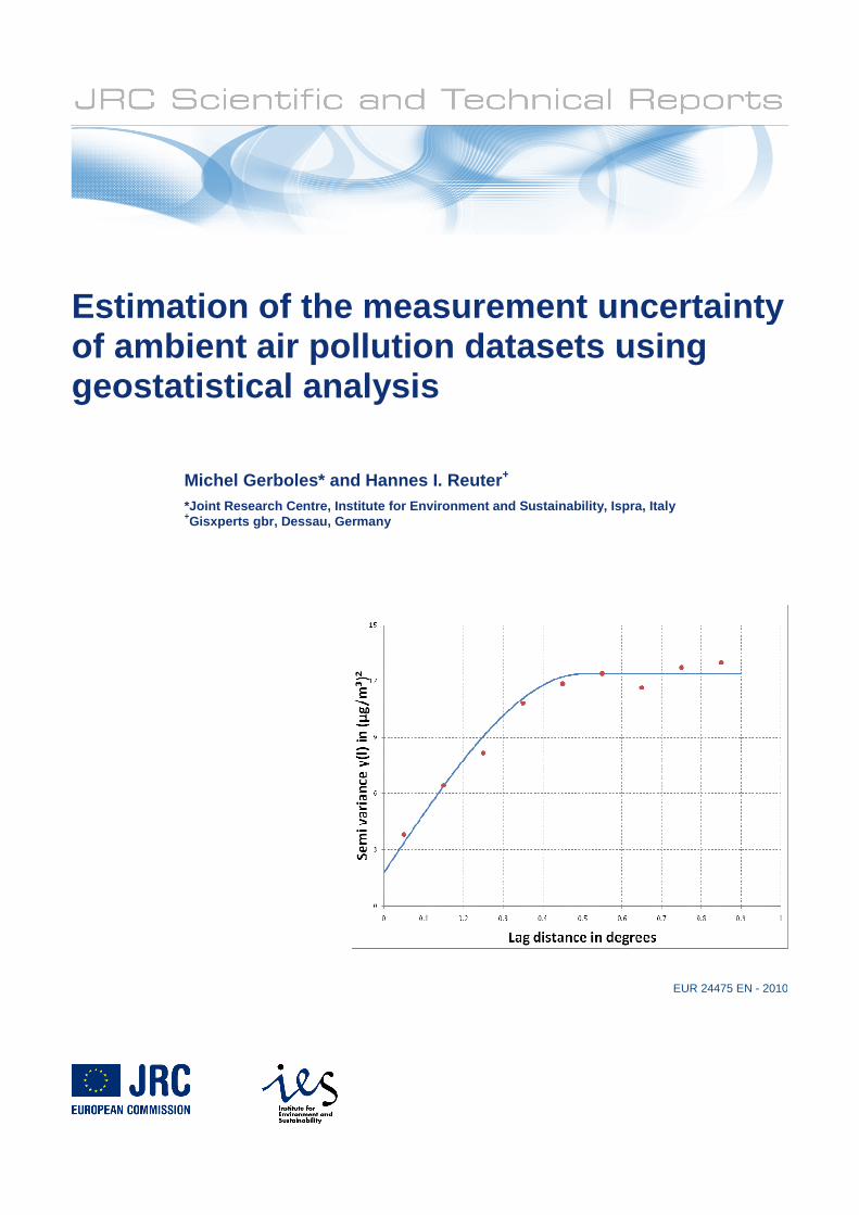
The graphical representation of the semi-variance γ(l) as a function of the distance is the semi-

variogram or variogram (see an example of variogram in Figure 2). Its main parameters are: nugget,

sill and range.

The semi-variograms obtained from experimental data often have a positive value of intersection with

the semi-variance axis called the nugget variance or nugget. From this point, the semi variance

increases until the variances of the data, called sill, is reached. Up to this point, the regionalized

variables in the sampling locations are correlated. They must be considered to be spatially independent

at higher distances than this point, called range. The sill is the variogram value at distances beyond the

range and, generally, it equals or approaches the population variance. The range provides the distance

beyond which variogram values remain constant.

An experimental semi variogram is modelled by fitting a simple function to the data pairs li, γ(l i).

Linear, spherical or exponential models are often used [10]: The spherical model is the most

commonly used one (see Equation 2). For example, a spherical model is fitted to the experimental data

of the variogram shown in Figure 2.

( )[ ]

+=>−+=≤

10

310

)(

5.05.1)(

CClalif

CClalif al

al

γγ

Equation 2

Where C0 is the nugget variance, C1 is the difference between the Sill C and the nugget variance C0 (C

= C0 + C1), l is the lag distance and a is the range.

The nugget effect is the value of the theoretical variogram C0 at the origin of the variogram (h → 0)

and is thus unknown. The empirical nugget is estimated by extrapolating the empirical variogram

towards h=0. It consists of the short-scale gradient of concentrations in the pollutant at distances much

shorter than the sampling distance or called micro-scale variation and of a stochastic measurement

10

uncertainty mainly the sampling and analytical variability, which should be true uncorrelated random

noise [10]. The nugget variance s2nugget can be expressed using Equation 3:

222scmeasnugget sss +=

Equation 3

where s2meas is the variance associated with the sampling and analytical variability and s2sc is the

variance due to micro-scale variability. Equation 3 is based on the assumption that s2meas and s2sc are

not correlated. In fact, for some atmospheric parameters, small changes in location can cause

significant changes in the concentration level of the pollutant. For example, if one moves from a ridge

to a valley, pollution may change quickly and at a scale at which we cannot predict because of sparse

observations.

10 Isaak, E. H., Srivastava, R. M., 1989, An Introduction to Applied Geostatistics. Oxford University Press, New York.

Figure 2: Example of a semi-variogram for PM10 stations in Europe, showing the nugget (local spatial variability and measurement uncertainty), the range (the extent of spatial variability) and the sill (the total variability in the dataset or the given extent). The gray line represents a example of a fitted semi-variogram function.

80

20

40

60

0 0.5 1.5 1.0

Sill C = C0 +C1

Se

miv

ari

an

ce γ

(l)

in µ

g/m

³

Lag Distance in Degrees

11

The estimated value of s2nugget cannot be decomposed in measurement error variance s2

meas and micro-

scale variance s2sc without further information or prior belief. However, the square root of s2

nugget

overestimates the uncertainty of measurement according to the extent of s2sc, the micro-scale variance.

It is then necessary to control the micro-scale variance so that the nugget variance, used as a surrogate

of the uncertainty of measurement, will only slightly overestimate the nugget variance. In this study,

the micro-scale variance is minimized by determining the nugget variance of subsets of all available

sampling sites selected according of their classification: background, traffic and industrial stations in

order to minimize the micro-scale variance.

The nugget variance is estimated by the intersection of the fitted model with the Y-axis of the

variogram. However, fitting different model (linear, spherical, exponential, power or a combination of

these) to the same experimental data set would have resulted in estimating different values for the

same nugget variance. Even more, fitting different type of models to different data sets would have

ended up in nugget variances that would have not been comparable anymore. In order to be consistent

in the method used to estimated the nugget variance of several data sets and hence be able to compare

them, it was decided to always fit a spherical model to all the prepared variograms.

When the uncertainty of measurement is determined using the direct approach, one starts by listing all

the possible contribution arising from different parameters (sampling, calibration ...) to be able to

combine them afterwards. One nice feature of estimating uncertainty using the nugget variance is that

all these contributions can be included by selecting appropriate sets of sampling sites that would

include different type of sampling lines, method of measurements/maintenance/calibration, equipment

brand, etc. The simple fact to select different sets of the sampling sites results in a wider estimation of

all parameters contributing to the uncertainty of measurements.

However, one should always keep in mind that there is a risk to attribute some contribution of the

micro-scale variation to the uncertainty of measurements and that this micro-scale variance might be

magnified by the heterogeneity of the sampling sites.

Notably one type of parameter contributing to the uncertainty of measurement that cannot be detected

by the nugget Variance consists in systematic bias that would be present at all sampling sites e.g. a bias

of the measurement methods or chemical interference. The presence of this type of systematic bias in

all the selected stations is nevertheless highly unlikely because of the very diverse implementation of

sampling, analytical and calibration methods managed by different laboratories implementing different

QA/QC procedures for a whole set of monitoring stations.

Finally, the method of estimation of the uncertainty of measurement proposed in this study relies on

the modelling of the variogram based on the data pairs consisting of lags and semi variances. The

12

nugget variance will depend on the semi-variance at the smallest lag distance of each variogram. When

the nugget variance is estimated per country using data sets whose smallest lag are different per

country, one cannot exclude a lack of homogeneity of the extrapolation of the spherical model on the

Y-axis.

Development of a methodology for downloading geo-referenced air pollution data series of AirBase and automatic estimation of the nugget variance of their variogram;

A PostgresSQL DB V8.3 was installed on a 64bit Ubuntu 9.4 distribution (http://www.ubuntu.com/)

with 8 GB RAM and 4 processors. Data were loaded using a self developed shell script (see Appendix

II: Developed Shell Script for Data import into the PostgresSQL Database), which automatically

loaded data if their measurement quality flag available in AirBase was set to 1. Each data record was

characterized using sample date, measurement value, station code and component code. For

performance issues each component was indexed on time and station code. Station data locations were

converted into a shapefile and loaded directly into Postgress. Indexing was performed on station code

and the geometry column. Several iterations where performed to determine which combination of

index / requests delivered the fastest return of data.

For further data analysis, the open source software R V 2.8.1 (www.r-project.org) with several

extensions (Rdbi + RdbiPgSQL for Database access, gstat, sp, automap for semi-variogram

calculations) has been used. Out of this analysis, a whole toolbox of algorithms (see Appendix I:

Developed R- Routines) has been developed which allow to process and calculate different kinds of

analysis (e.g. raw and fitted semi-variograms, outlier calculation, general statistics and fitted functions

to the time series), all with respect to the analysis of the air quality datasets. In general, the data

analysis consisted of three different steps: loading the data from the DB into memory, performing the

necessary calculations, writing semi-variogram results into ASCII files for further analysis.

Data connections between R and the Postgress DB have been established using the RDBI driver. The

time of this driver delivering data is approx 2% compared to the time the ODBC Database drivers

would deliver data. Stations were selected, joined with the corresponding location data table and

imported into R. All datum data were converted into Julian day to be able to perform temporal and

spatial selections. If data needed to be normally distributed for applying the outlier test (see below), a

natural logarithmic transformation was performed. Additionally, to improve mathematical stability, an

offset has been added before the log transformation derived by the absolute minimum value of the

dataset + 0.5 to avoid undefined values (a log of zero or of negative values is not defined).

13

Semi-variogram analysis was performed using an automatic semi-variogram fitting provided by the

automap toolbox (Hiemstra et al, 2008) [11]. This toolbox was adapted by limiting the maximum lag

distance to a total search radius of 2° of latitude and longitude corresponding to ~ 220 km long. This

method automatically could test/fit different semi-variogram models and fits semi-variogram

parameters based on a given dataset. Usually, the algorithm determines the boundaries for the lags by

determining the spatial boundary and dividing it by the size of the area. However, as the distribution of

stations is clustered, this algorithm delivered at times lag boundaries, which were not corresponding to

the spatial autocorrelation of the underlying data. For example, fitting lag distances to Spanish data

without limits resulted in a maximum lag distance of ~10° due to some stations on the Canary Islands

as well as on the mainland. By introducing a limiting factor, the spatial variability of the mainland

which should have been up to a maximum of ~2° for Spain could be maintained. Another typical

example is given by stations placed behind a mountain range, while all other stations form a cluster.

Therefore, we let the algorithm estimated the boundaries, while limiting the maximum distance to

preset value of 2°. Thereby we effectively ensured that the lag boundaries where always within the

autocorrelation range.

In the beginning of the analysis, a couple of hundred semi-variograms were computed: It became clear

that outliers influenced the semi-variogram calculation, which rendered analysis of spatial dependency

11 Hiemstra, P.H., Pebesma, E.J., Twenhöfel, C.J.W and G.B.M. Heuvelink (2008). Automatic real-time interpolation of radiation hazards: a prototype and system architecture considerations. International Journal of Spatial Data Infrastructures Research, vol 3, p 58-72

Figure 3: Several methods to detect outliers in 3D datasets (Figure taken from Chang-Tien Lu[12] )

14

using semi-variance analysis questionable. The outliers influenced the fitting of the semi-variogram

function and led to an artificial increase of the nugget effect.

Therefore an outlier procedure was implemented based on already existing literature. Chang-Tien Lu

[12] have outlined and classified several algorithms [13,14,15,1617,18,19,20,21] as seen in Figure 3.

Two families of outlier detection methods can be distinguished. First the ones which calculates statistic

of the distribution of pollutant in one dimension and ignore geographical location [14, 16]. The second

family, the spatial-set outlier detection methods, consider both attribute values and spatial

relationships. Within this family we used the “Smooth Spatial Attribute method” [12] that was

developed for the identification of outliers in traffic sensors. This method is thought to be fit for the

identification of outliers in a given homogeneous dataset of air quality data that represents in a similar

way a quantity measured in time and space.

The Smooth Spatial Attribute method relies on the definition of a neighbourhood for each air pollutant

measurement. It corresponds to a spatio-temporal domain limited in time (+/- 1 day) and distance (+/-

1 degree) around location x. The neighbourhood is better understood by observing the diagram in

Figure 4. The objective of the method is that within a given spatio-temporal domain in which the value

of the attribute values of neighbours have a relationship due to the distribution/transport/emission and

reaction of air pollution, outliers will be detected by extreme value of their attribute value compared to

the attribute value of their neighbours. The main computation cost of the method is dominated by disk

Input/Output cost and the main constrain of the method is the normality of the distribution of the

attribute values of neighbours.

In the following text, we called x the concentration of a pollutant or its location. Within each

neighbourhood, several measurements of the same compounds at different locations and time xxi,yi are

12 Chang-Tien Lu, Dechang Chen, Yufeng Kou, "Detecting Spatial Outliers with Multiple Attributes," ictai, pp.122, 15th IEEE International Conference on Tools with Artificial Intelligence (ICTAI'03), 2003. 13 M. Ankerst, M. Breuning, H. Kriegel and J. Sander. Optics: Ordering points to identify the clustering structure in Proceedings of the 1999 ACM SIGMOD International Conference on Management of Data, Philadelphia, Pennsylvania, USA, pages 49-60, 1999. 14 V. Barnett and T. Lewis. Outliers in Statistical Data. John Wiley, New York, 3rd Ed. 1994. 15 M. Breuning, H. Kriegel, R. T. Ng and J. Sander. OPTICS-OF: Identifying Local Outliers in Proc. Of PKDD ’99, Prague, Czech Republic, Lectures Notes in Computer Science (LNAI 1704), pp 262-270, Springer Verlag, 1999. 16 R. Johnson. Applied Multivariate Statistical Analysis, Prentice Hall, 1992. 17 E. Knorr and R. Ng. Algorithms for Mining Distance-Based Outliers in Large Datasets in Pric. 24th VLDB Conference, 1998. 18 M. Kraak and F. Ormeling. Cartographer: Visualization of Spatial Data. Longman, 1996 19 F. Preparata and M. Shamos. Computational Geometry: An Introduction. Springer Verlag, 1998. 20 I. Ruts ans P. Rousseeuw. Computing Depth Contours Of Bivariate Point Clouds. In Computational Statistics and Data Analysis, 23:153-168, 1996. 21 D. Yu, G. Shekholeslami and A. Zhang. Findout: Finding Outliers in Very Large Datasets. In Department of Computer Science and Engineering State University of New York at Buffalo Buffalo, Technical report 99-03, http://www.cse.buffalo.edu/tech-reports/, 1999.

15

available. Equation 4 allows computing a weighted average of all available measurements xxi,yi within

each neighbourhood where the weights correspond to the inverse spatial and time distance between

xxi,yi and x.

After a log-transformation of non - Gaussian data within any neighbourhood, we computed the

differences Sx between value at x and the average of its neighbourhood for each measurement

according to Equation 5.

ii yx

n

iyx xwx ∑=1

, Equation 4

yixixfxSx

,−=

Equation 5

s

xxz i

i

−= Equation 6

θ>iz Equation 7

Then within each neighbourhood, the Sx values were normalised to center data at 0 with a standard

deviation of 1 using Equation 6 in which x and s are the weighted average and weighted standard

deviation of all possible Sx values within any neighbourhood. Finally, the test for detecting an outlier,

given in Equation 7, searches for zi values exceeding a threshold value consisting in the moving

average of five consecutive zi values plus a threshold value of 2 corresponding to a confidence interval

Figure 4: Spatial and temporal outliers – definition of neighborhood [12]

16

in which 95 % of zi values would lay. In contrast to the paper by Lu [12], we did not use an absolute

value of the z-transformation due to the fact that the sign of the outlier is of interest to us as we want to

understand if a station is measuring to low quantities or to high quantities compared to the its

neighbourhood stations with the same classification (urban, background, traffic ..). By plotting the

result of the zi against the moving average of the z- plus the threshold value, outliers were identified.

An example is given in Figure 5 for an Austrian station monitoring PM10 with the identification of 19

outliers of daily values in 2007.

17

Finally, the methodology developed for the estimation of the uncertainty of measurement based on the

nugget variance can be described by the flow chart given in Figure 6.

Figure 5: Outlier analysis for Austrian Station AT0227A (Großenzersdorf/Glinzendorf) using the developed method. The Station Values (black circles) are shown with the average of the surrounding stations circle(red line) +/- 2 standard deviation (SD) (Top Left), the histogram of the (log transformed) measurement value for normality (Top Right); the Sx values for the station (black) with respect to the surrounding Mean (Red) and SD(blue)(Middle Left); the Quantile distribution of the Sx values (Middle Right) to see if the distribution contains any large deviations; the zi values of the station (black) plotted against the specified threshold (Lower Left); and in the lower right corner the average number of stations in the surrounding used for the calculations and the number of identified outliers out of one year .

18

If more than 20 stations were available at any given time step (e.g. day), a semi-variogram analysis

was performed consisting of a nugget effect and a spherical model. An example of the effect of

discarding outliers producing a decrease of the nugget effect and sill is presented in Figure 7 for the

rural background station in Germany for PM10 in 2007.

Download data from Airbase

Import data into database

Select monotoring station per country,component, year, station type and area

type

Outlier test based on average space(2º = 220 km) and time ±/- 1 day

Compute variogram including nuggeterror and spherical model

Extract nugget variance,range and sill

Add nugget, range and sill to table ofresults

Figure 6: Flow chart representing the different steps of the developed methodology for the estimation of uncertainty of measurements

19

Estimation of the measurement uncertainty using the nugget variance For PM10, our pollutant of interest, the number of monitoring stations increased in all countries

whatever station or area type as shown in Table 1. In 2007, Germany had a total of 358 stations

(among which 155 traffic stations in urban areas), France had 238 stations (among which 126

background stations in urban areas), Italy had 141 stations (among which 86 traffic stations in urban

areas) and Austria had 87 stations with 59 background stations in urban areas. The number of stations

included for which data are present in AirBase for all possible combination of station and area type is

given in Table 2. As the micro micro-scale variability estimated form the geostatistical analysis of

Industrial stations was expected to be higher than with urban and industrial stations, it was decided not

to select this type of station in the analysis.

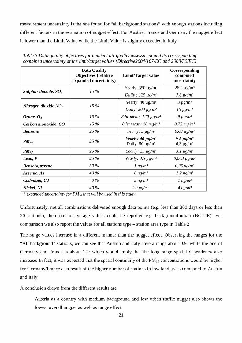
As mentioned in Introduction, the European Directives defines data quality objectives (DQOs) that

represent the highest allowed expanded uncertainty of measurements in percentage of the Limit Value.

Table 4 gives for each pollutant the combined uncertainty in µg/m³ corresponding to this percentage.

For PM10, we will remember that the combined uncertainty corresponding to the European Data

Quality Objective is 5 µg/m³.

For Year 2007, we calculated the averages of all daily measurement uncertainties estimated by the

square root of the nugget variance and ranges of the semi-variograms for different station and area

types for Austria, (AT), Germany (DE), France (FR) and Italy (IT). The values are given in Table 4.

Figure 7: Decrease of the nugget effect and sill of the semi variogram for Julian Day 17176 in Germany on rural background stations by discarding outliers (left all monitoring stations are used, right outliers are discarded)

20

Table 1: Number of Stations for the most abundant parameters of AIRBASE in 2002 and 2007 for traffic (TR) and background (BG) type stations for urban (UR), rural (RU) and suburban (SU) areas.

SO2 O3 NO2 PM10

AT DE FR IT AT DE FR IT AT DE FR IT AT DE FR IT

20

07

TR-UR 31 94 7 27 2 47 29 26 44 196 28 155 27 86

BG-RU 87 1 21 50 69 62 41 34 11 30 37 19 52 11 8

BG-UR 49 1 42 17 82 164 69 22 14 183 90 20 86 126 31

BG-SU 52 5 25 23 72 147 41 24 27 115 48 20 65 74 16

20

02

TR-UR 58 29 6 41 6 18 27 19 39 41 15 84 26 17

BG-RU 103 2 6 53 72 53 15 37 9 36 13 12 35 11 -

BG-UR 55 2 15 18 92 130 21 23 19 147 21 9 79 101 10

BG-SU 54 1 10 21 84 136 19 22 36 119 12 11 52 70 -

Table 2: Classification of station and area in Austria, Germany, France and Italy.

Station type Area type Number of station Station type Area type Number of station

Industrial suburban 524 Background urban 1658

Industrial urban 263 Background suburban 1213

Industrial * 1 Background unknown 35

Industrial unknown 17 Background rural 814

Industrial rural 298 Unknown rural 2

Traffic unknown 5 * * 4

Traffic suburban 248 Unknown unknown 32

Traffic urban 1493 * suburban 1

Traffic rural 44 Unknown urban 67

Stars denote missing station types.

First of all, they are consistent with the expected uncertainty in field. They are generally lower than the

data quality objective expressed as combined uncertainty of the Limit Value (5 µg/m³). It is likely that

the estimation of the measurement uncertainty using traffic type station is overestimated by a micro-

scale variation included in this type of station. For urban traffic, Austria shows the lowest values for

nugget, followed by Germany and France with double the amount effect. Italy shows the highest

amount for the nugget.

Background stations do not show such clear patterns. The nugget values of Austria are double

compared to the observed values for Germany and France; while Italy shows nearly three fold values

of these nuggets. The reason for the nugget differences is unclear. A clear attribution to different

station networks or different traceability of standard strategies seems not be possible but should be

investigated. A second factor could be the different spatial distributions of the station networks for

background stations influencing the computed results. We believe that the best estimated of the

21

measurement uncertainty is the one found for “all background stations” with enough stations including

different factors in the estimation of nugget effect. For Austria, France and Germany the nugget effect

is lower than the Limit Value while the Limit Value is slightly exceeded in Italy.

Unfortunately, not all combinations delivered enough data points (e.g. less than 300 days or less than

20 stations), therefore no average values could be reported e.g. background-urban (BG-UR). For

comparison we also report the values for all stations type – station area type in Table 2.

The range values increase in a different manner than the nugget effect. Observing the ranges for the

“All background” stations, we can see that Austria and Italy have a range about 0.9º while the one of

Germany and France is about 1.2º which would imply that the long range spatial dependency also

increase. In fact, it was expected that the spatial continuity of the PM10 concentrations would be higher

for Germany/France as a result of the higher number of stations in low land areas compared to Austria

and Italy.

A conclusion drawn from the different results are:

Austria as a country with medium background and low urban traffic nugget also shows the

lowest overall nugget as well as range effect.

Table 3 Data quality objectives for ambient air quality assessment and its corresponding combined uncertainty at the limit/target values (Directive2004/107/EC and 2008/50/EC)

Data Quality Objectives (relative

expanded uncertainty) Limit/Target value

Corresponding combined

uncertainty

Sulphur dioxide, SO2 15 % Yearly :350 µg/m³

Daily : 125 µg/m³

26,2 µg/m³

7,8 µg/m³

Nitrogen dioxide NO2 15 % Yearly: 40 µg/m³

Daily: 200 µg/m³

3 µg/m³

15 µg/m³

Ozone, O3 15 % 8 hr mean: 120 µg/m³ 9 µg/m³

Carbon monoxide, CO 15 % 8 hr mean: 10 mg/m³ 0,75 mg/m³

Benzene 25 % Yearly: 5 µg/m³ 0,63 µg/m³

PM10 25 % Yearly: 40 µg/m³ Daily: 50 µg/m³

* 5 µg/m³ 6,3 µg/m³

PM2,5 25 % Yearly: 25 µg/m³ 3,1 µg/m³

Lead, P 25 % Yearly: 0,5 µg/m³ 0,063 µg/m³

Benzo(a)pyrene 50 % 1 ng/m³ 0,25 ng/m³

Arsenic, As 40 % 6 ng/m³ 1,2 ng/m³

Cadmium, Cd 40 % 5 ng/m³ 1 ng/m³

Nickel, Ni 40 % 20 ng/m³ 4 ng/m³

* expanded uncertainty for PM10 that will be used in this study

22

Italy, shows the largest nugget parameters across all combinations. The reason for this is still

unclear.

Station classification appears to influence the nugget and range results in different MS in

various degrees - a more precise classification delivers an increased spatial dependency

The spatial distribution of the station network (e.g. the Austrian/Italian Mountain Valley

situation versus a German/France lowland situation) might have influenced the quantified

nugget and range values as well. However the size of this effect is uncertain.

23

Table 4 Averaged Daily Nugget and Range Values for the year 2007 for the EU Member states Austria (AT), Germany (DE),France (FR) and Italy (IT) for the Station Type - Station Area Type Combinations Traffic-Urban (TR-UR), Background-rural (BG-RU), Background-Urban (BG-UR), Background-Suburban (BG-SU), all Background stations (BG-ALL), and all stations (ALL-ALL).

Station Combination Nugget and Range Values for the Year 2007 for PM10

St - Iso AT DE FR IT

Nug

get i

n µ

g/m

³

TR-UR 3.8 5.5 5.3 9.3

BG-RU 1.9

BG-UR 2.8 1.6 7.5

BG-SU 1.9 1.9

BG-ALL 4.0 2.7 3.1 7.0

ALL-ALL 4.2 6.1 6.2 8.9

Ran

ge in

sph

eric

al d

egre

es TR-UR 0.93 1.22 1.06 1.20

BG-RU 1.19

BG-UR 1.06 0.91 1.10

BG-SU 0.94 1.16

BG-ALL 0.9 1.17 1.2 0.89

ALL-ALL 0.91 1.01 1.16 1.11

24

Trend over time of the measurement uncertainty indicated by the nugget effect While the results for year 2007 give only a short snapshot in time, we investigated how the nugget and

range change over time. The same geostatistical analysis as for year 2007 was performed over the

timeframe 1997-2007.

By plotting the nugget effect of PM10versus time, it is possible to observe that the slope of regression

line (-0,002) for Germany (see Figure 8) shows a decrease that indicates a slight improvement of the

measurement uncertainty between 1997-2007. The same decrease of measurement uncertainty is

stronger for Austria as shows the slope of the nugget variance versus time (-0,010, see Figure 9).

However one should note that the initial nugget variance of Austria in 1997 was higher than the one of

Germany. This is evidenced by the intercept of Austria of 213, compared to 45 for Germany (see

Figure 8 and Figure 9). Figure 8 also shows an annual effect of changes in spatial distribution in

Austria that is clearly visible in the yearly increase in small scale variability (i. e. nugget effect) during

the winter months.

Figure 8: Nugget Semi-variance (gray circles) plotted versus Time (Julian Day) for all German Background Stations over the timeframe 1997-2007. The red line indicates a linear model fit for the plotted data; the parameters shown in the centre of the figure.

25

Figure 9: Nugget Semi-variance (gray circles) plotted versus Time (Julian Day) for all Austrian Background Stations over the timeframe 1997-2007. The red line indicates a linear model fit for the plotted data; the parameters shown in the centre of the figure

A more general picture for the different stations types can be found using simple linear regression

analysis as shown in the Table 5. In general we observe a decrease in small scale variability across all

years. For the “All background stations (line BG-ALL)”, a negative coefficient can be observed.

Certainly, the values are rather small considering the fact that 10 years of observations are taken into

account. While Germany has the smallest decrease in the nugget effect with time (e.g. the least

reduction in small scale variability), we could observe Austria and France had similar decreasing

values. The largest decrease could be observed for Italy (fourfold over that from Austria).

For the Urban Traffic combination the results are different. We see the strongest decrease in the

Austrian dataset, followed by Germany and Italy. Interestingly, France showed an increase in small

scale variability with years which need further investigation.

Range effects for “All background stations” (e.g. the length of the spatial dependency) are actually

increasing for Germany and slightly increasing for France, while decreasing for Austria and slightly

decreasing for Italy. This might indicate that the stations with an increasing range show a more

homogeneous picture of the air quality situation surrounding it. In fact, it might be due to an increase

of QA/QC actions performed over the years. It could also be the result of a change in the nature or

quantity of air pollution emissions/transport or reactions over the year. Another reason might be the

26

increase/decrease of number of monitoring stations or change in the station classifications. For traffic

stations, such statement cannot be made. We observed increase in ranges for Austria, Italy and

Germany ans significant decrease for France.

Table 5 Coefficients for fitted linear models for nugget and Range Values for Austria (AT), Germany (DE), France (FR) and Italy (IT) for the Station Type - Station Area Type - Combinations Traffic-Urban(TR-UR), Background-rural(BG-RU), Background-Urban(BG-UR), Background-Suburban(BG-SU), All Background stations (BG-ALL).

Slope of regression lines over 10 years

St - Iso AT DE FR IT

Slo

pe in

% fo

r nu

gget

TR-UR -1,8 % -0,2 % 0,6 % 0,0 %

BG-RU -0,8 %

BG-UR -0,6 % -1,6 % -1.9 %

BG-SU -0,2 % -1,7 %

BG-ALL -1,0 % -0,2 % -1,2 % -4,3 %

Slo

pe in

% fo

r R

ange

TR-UR 12,2 % 2,8 % -6,0 % 4,0 %

BG-RU 2,0%

BG-UR 3,3% -5,9 % 5,8 %

BG-SU 1,7% -1,4 %

BG-ALL -2,8 % 2,6% 1,0 % -1,0 %

All the semi-variograms of Germany between 1997 and 2007 are shown in Figure 10. Along the x-axis

the Julian Day is shown, while in y direction the lag distances are plotted. The height of each cross

displays the semi-variance for background stations in rural area. Additionally, a surface is plotted

inside the figure that fits all points in the semi-variograms. This surface gives a linear model with

respect to the time and the distance. For Germany and rural background stations, a clear decreasing

trend can be observed for the nugget effect as well as for the semi-variogram range.

27

Figure 10: The raw semi-variogram plotted versus Julian day. The x-axis shows the Julian day; the y-axis shows the lag distance; the z-axis the calculated semi-variance. The surface inside the 3D plot represents a fitted model of the semi-variance versus julian day and lag distance; while parameters of these equation are shown at the bottom part of the figure. Black crosses indicates higher values than black crosses.

Create a warning system for classification of monitoring stations For the identification of environments responsible for population exposure we applied the functions

developed in the outlier detection methodology. An example from the results is shown in Table 6. We

classified every single measurement that exceeded our conservative threshold of 2. The identified

outliers as well as the given percentages are similar for urban and rural areas in Austria. For Germany,

quite some significant difference can be observed as almost 2 % of the urban stations measurements

28

are detected as outliers, similar to the Austrian data. However, Germany's rural background station

data show a very low number of outliers.

Table 6 General Statistics of number of records, identified outliers and percentages of outliers identified for four different station type - station area type combinations

Station Type Number of Records Identified Outliers Percentage Outliers

DE Background rural 38480 27 0.07

DE Background urban 63906 1259 1.97

AT Background rural 13339 331 2.48

AT Background urban 13990 352 2.52

Based on these data we divided the stations with respect to their average zi values in 4 classes. For

example, for the background data shown in the table above, the four classes are delimited by: low-level

stations (bg, with z < -1), stations below average (ba, with -1<z<0), above average(aa, with 0<z<1),

and high level stations stations(nb with z>1). Examples for the four cases are shown in Figure 11 to

Figure 14. For the rural background type, stations which are classified as high level stations should be

examined further and a reclassification of the station type and of the station area type should be

considered if appropriate. It should be stressed that the proposed methodology is a first preliminary

assessment, which needs expert validation from the local station managers to see if the assignment

needs to be changed. The same is valid for urban background stations which are classified as bg

stations – a reclassification as rural background stations might be appropriate. However, more

investigations have to be performed to include actual population density data as well as more in depth

investigations to quantify the differences in population exposure measurements and the ambient air

measurements to come to a sound scientific assessment.

29

Figure 11: Classification of station for Austria for the rural station type for PM10. Station Labels without points are positions where no classification has been performed

30

Figure 12: Classification of station for Austria for the urban station type for PM10. Station Labels without points are positions where no classification has been performed.

31

Figure 13: Classification of station for Germany for the rural station type for PM10. Station Labels without points are positions where no classification has been performed

32

Figure 14: Classification of station for Germany for the urban station type for PM10. Station Labels without points are positions where no classification has been performed

33

Conclusions We developed a methodology able to automatically estimate the measurement uncertainty in the air

pollution data sets of AirBase. The figures estimated with this method were consistent with

expectations from laboratory and field estimation of uncertainty and with the Data Quality Objectives

of the European Directives.

The proposed method based on geostatistical analysis is not able to estimate directly the measurement

uncertainty. It estimates the nugget effect together with a micro-scale variability that must be

minimized by accurate selection of the type of station. Based on the results obtained so far, it is likely

that measurement uncertainty is best estimated using all background stations of whatever area type.

So far the methodology has been used to estimate uncertainty in 4 different countries independently.

This work should be continued for the whole Europe or for background station without national

borders. The method has been shown to be also useful to compare the spatial continuity of air pollution

in different countries that seems to be influenced by the topography of each country.

Moreover, it may be used to quantify the trend of measurement uncertainty over long periods like

decades with the possibility to evidence improvement in the data quality of AirBase datasets. Over the

last 10 years for Austria, Germany, France and Italy a decrease in the nugget effect can be observed,

while the change in range (long range spatial dependency) was not significant. Further investigations

are needed to determine if this decrease of nugget variance is caused by a decrease of the measurement

uncertainty or by long term variations of air pollution or other meteorological factors. We showed that

the nugget and range for PM10 in 2007 differed significantly between traffic stations while being more

or less consistent for all background station types sited in whatever area type. Traffic situations

showed up to twice higher nugget effects compared to background station scenarios. Data for different

seasons are computed. However more analysis is needed to clarify the results.

Thanks to the implemented outlier detection module, that could also be of interest as a warning system

when countries report their measurements to EEA, we have proposed a simple solution to investigate

34

station classifications in AirBase. We tested the method on the German and Austrian background

stations. For several stations, differences in classification could be identified which appeared with

respect to the inherent data properties of the selected dataset. However, validation of the outcome of

this module has to be performed thoroughly.

The developed method presents a number of shortcomings:

1. The nugget variance overestimates the uncertainty of measurement because of the micro-scale

variations and in case of lack of spatial continuity of the pollutant (river, island, mountains ...)

2. The micro-scale variance might be magnified/decreased by the heterogeneity/homogeneity of

the sampling sites.

3. The nugget variance cannot detect systematic bias e.g. bias of the measurement methods or

chemical interference. This type of systematic bias is unlikely if the selected sufficient

sampling sites have different sampling systems, analytical and calibration methods and

QA/QC.

4. The nugget variance will depend on the semi-variance of the smallest lag distance of each

variogram. When the nugget variance is estimated per country using data sets whose smallest

lag are different, one cannot exclude a lack of comparability with the extrapolation of the

spherical model on the Y-axis.

Seen the number of shortcomings of the method, validation of the method by comparison to direct

approach is needed. For now, this method can be used as a confirmation tool or a ranking tool.

Future study: Some points of the method need subsequent validation or modification:

� Optimization of the maximum lag distance of the variogram in order to strengthen the

estimation of the nugget effect, range and sill. Currently, we preset the maximum extent of the

boundaries for the semi-variogram analysis to effectively ensured that the lag boundaries were

always within the autocorrelation range. Further research has to investigate how the boundaries

35

could be fitted automatically also for different area size dataset.

� Optimization and validation of the parameters used for the outliers test (the limit of the

neighbourhood ± 1 day and ± 2º and the criteria for the z test: z average over 5 days ± 2). It

might be that the test threshold should be different for different components or location.

� Should the semi-variogram be plotted in absolute or in relative values on its y-axis? This is an

evaluation of the effect of local mean that may have an effect on the nugget, range and sill.

Study whether the uncertainty has a constant value for the whole range of concentration of

pollutant (i.e. like in our estimation) or is dependent of the level of concentration (i.e a

percentage of the concentration). The latter case is more likely, the variogram should thus be

built using the percentage of the concentration of pollutant versus the limit value.

� To diminish the contribution of the micro-scale variability to the nugget effect, explicative

variables known on the whole dominium with a high density should be included in

multivariable geostatistics like co-Kriging or Kriging with external drift.

� Setup a system to be able to spike air pollution data sets with signal noise (error), quantify the

effect on the nugget effect, range and sill in order to validate the whole methodology of

uncertainty estimation.

� Validation of the method by comparing its estimation of uncertainty with estimation carried out

with laboratory or field experiments. Another solution could be chosen by selecting variograms

with pure nugget error to estimate the measurement uncertainty and compare this value with

the one only estimated from background stations or against direct estimates of uncertainty with

the direct approach.

� Determine which subset of station type and area type to estimate these metrics. The actual

hypothesis is that the nugget variance should be estimated using all background stations which

lead to a low sill, long range and nugget variance near pure measurement error.

� Look for variables with high density values that are correlated with the concentrations of

pollutants (emissions, population density, number of buildings, models outputs ...). By

developing variogram of the detrended variables, the influence of the micro-scale variation on

the nugget variance might be deleted.

� Optimization of the outlier procedure in terms of computing speed to reach a near-to-real time

detection method that might be useful when countries report their data.

36

The computation of statistics and their evaluation needs be continued:

� Carry out the assessment of nugget variance, range and sill for other pollutants with sufficient

monitoring stations (eg. O3, NO2…) and for the averaging time of the monitoring for regulatory

purposes defined in the European Directives.

� The values of nugget variance should be investigated according to the type calibration chain of

standards and other QA/QC and sampling procedures that is implemented by each country or in

relation to the implemented inter-comparison exercises to check if these factors may influence

the nugget variance.

� The spatial continuity estimated using the range of variograms (the longer the range the more

stable the spatial distribution) should be investigated to evidence which compounds are more

affected by local emissions, reaction or log-range transport of pollutants.

� Evaluate the trend of nugget variance, sill and range of spatial continuity e.g. over the last 10

years.

� Investigate effect of season. While we have performed a time series analysis to establish how

the nugget and range effect changes over a ten year time frame, we already could see from our

analysis the influence of seasons. Still the question remains about how the seasonality

influences these results in a quantitative way. We should split up the 10 year dataset in steps of

3-4 month each (maybe using a cluster analysis) and analyze them separately. This is important

to evidence effects of the station density across different years and for a better understanding of

the uncertainty of the different contributing measurement networks of the AirBase Database.

� Estimate the sill, range and nugget variance by selecting monitoring stations belonging to more

than one country to detect the presence of possible clusters with borders.

� Map of number of outliers: by performing this in a consistent way across several components,

countries might be able to further streamline and improve their station monitoring network.

Based on the analysis performed in the classification of sampling sites for the year 2007, we

observed that different stations with respect to their station area type or their station type would

have to be reclassified. However, what is currently missing is the temporal domain. We

urgently need to re evaluate this kind of classification over a range of years to see if a

consistent pattern can be detected, otherwise no sound scientific advice can be given to

reclassify these stations.

37

Appendix I: Developed R- Routines

Appendix II: Developed Shell Script for Data import into the PostgresSQL Database

Please contact the Authors

European Commission

EUR 24475 EN – Joint Research Centre – Institute fo r Environment and Sustainability

Title: Estimation of the measurement uncertainty of ambient air pollution datasets using geostatistical analysis

Author(s): Michel Gerboles and Hannes I. Reuter

Luxembourg: Publications Office of the European Union

2010 – 37 pp. – 29,7 x 21,0 cm

EUR – Scientific and Technical Research series – ISSN 1018-5593

ISBN 978-92-79-16358-6

doi:10.2788/44902

Abstract

We developed a methodology able to automatically estimate of measurement uncertainty in the air pollution data sets of AirBase. The figures produced with this method were consistent with expectations from laboratory and field estimation of uncertainty and with the Data Quality Objectives of European Air Quality Directives. The proposed method based on geostatistical analysis is not able to estimate directly the measurement uncertainty. It estimates the nugget effect from variogram modelling together with a micro-scale variability which must be minimized by accurate selection of the type of station. Based on the results obtained so far, it is likely that measurement uncertainty is best estimated using all background stations of whatever area type. So far the methodology has been used to estimate measurement uncertainty in datasets from 4 different countries independently. This work should be continued for the whole Europe or for background station without national borders. The method has been shown to be also useful to compare the spatial continuity of air pollution in different countries that seems to be influenced by the spatial distribution of the stations (e.g influenced by topography) of each country.

Moreover, the method may be used to quantify the trend of measurement uncertainty over long periods (decades) with the possibility to evidence improvement in the data quality of AirBase datasets.

The implemented outlier detection module would be of interest as the warning system when countries report their measurements to the European Environment Agency. The method could also provides a simple solution to investigate the assignment and accuracy of station classification in AirBase.

How to obtain EU publications

Our priced publications are available from EU Bookshop (http://bookshop.europa.eu), where you can place an order with the sales agent of your choice.

The Publications Office has a worldwide network of sales agents. You can obtain their contact details by sending a fax to (352) 29 29-42758.

The mission of the JRC is to provide customer-driven scientific and technical support for the conception, development, implementation and monitoring of EU policies. As a service of the European Commission, the JRC functions as a reference centre of science and technology for the Union. Close to the policy-making process, it serves the common interest of the Member States, while being independent of special interests, whether private or national.

LB

-NA

-24475-EN

-C