and Physics Modelling tracer transport by a cumulus ... Physics Modelling tracer transport by a cumulus ensemble: lateral boundary conditions and large-scale ascent M. Salzmann1, M

Atmos. Chem. Phys., 4, 1797–1811, 2004www.atmos-chem-phys.org/acp/4/1797/SRef-ID: 1680-7324/acp/2004-4-1797

AtmosphericChemistry

and Physics

Modelling tracer transport by a cumulus ensemble: lateralboundary conditions and large-scale ascent

M. Salzmann1, M. G. Lawrence1, V. T. J. Phillips2, and L. J. Donner2

1Max-Planck-Institute for Chemistry, Department of Atmospheric Chemistry, PO Box 3060, 55020 Mainz, Germany2Geophysical Fluid Dynamics Laboratory, NOAA, Princeton University, PO Box 308, Princeton, NJ 08542, USA

Received: 10 May 2004 – Published in Atmos. Chem. Phys. Discuss.: 22 June 2004Revised: 31 August 2004 – Accepted: 3 September 2004 – Published: 13 September 2004

Abstract. The vertical transport of tracers by a cumulusensemble at the TOGA-COARE site is modelled during a7 day episode using 2-D and 3-D cloud-resolving setups ofthe Weather Research and Forecast (WRF) model. Lateralboundary conditions (LBC) for tracers, water vapour, andwind are specified and the horizontal advection of trace gasesacross the lateral domain boundaries is considered. Fur-thermore, the vertical advection of trace gases by the large-scale motion (short: vertical large-scale advection of tracers,VLSAT) is considered. It is shown that including VLSATpartially compensates the calculated net downward transportfrom the middle and upper troposphere (UT) due to the massbalancing mesoscale subsidence induced by deep convec-tion. Depending on whether the VLSAT term is added ornot, modelled domain averaged vertical tracer profiles candiffer significantly. Differences between a 2-D and a 3-Dmodel run were mainly attributed to an increase in horizon-tal advection across the lateral domain boundaries due to themeridional wind component not considered in the 2-D setup.

1 Introduction

Deep convective clouds can rapidly transport trace gasesfrom the lower troposphere to the upper troposphere (e.g.Gidel, 1983; Chatfield and Crutzen, 1984; Dickerson et al.,1987; Pickering et al., 1990) where in many cases theirchemical lifetimes are longer and horizontal winds often arestronger. On the other hand, tracers are transported down-wards due to the mass balancing mesoscale subsidence in-duced by deep cumulus clouds and due to downdrafts insidedeep convective clouds. Both upwards as well as downwardstransport have been found to influence global budgets of im-

Correspondence to:M. Salzmann([email protected])

portant trace gases such as ozone (Lelieveld and Crutzen,1994; Lawrence et al., 2003).

In recent years cloud-resolving models (CRMs) have beenused by numerous investigators to study the transport of trac-ers (e.g. Scala et al., 1990; Wang and Chang, 1993; An-dronache et al., 1999; Skamarock et al., 2000; Wang andPrinn, 2000; Pickering et al., 2001; Ekman et al., 2004). Ineach of these studies the evolution of a single deep convec-tive storm was simulated. Lu et al. (2000) presented the firstmulti-day 2-D model study of trace gas transport by a cumu-lus ensemble. They applied periodic lateral boundary con-ditions (PLBC) and observed large-scale advection (LSA)terms for water vapour and potential temperature, but ne-glected the corresponding terms for tracers. Particularly insituations with vertical wind shear, model calculated tracerfields obtained with PLBCs will not necessarily be meaning-ful if the model is run longer than the timeτadv=L/vmax

it takes the tracer to be advected across the entire length ofthe domain and the tracer’s chemical lifetime is longer thanor comparable toτadv. Herevmax=max(v(z)) is the maxi-mum domain averaged horizontal wind speed, andL is thehorizontal domain length. On the other hand if LBCs fortrace gases and for the wind are specified, the horizontalwind is allowed to change the vertical tracer gradients andthus the vertical transport. In this study a framework is pre-sented which enables investigators to drive cloud-resolvingchemistry transport models with observed data for longer pe-riods taking into account large-scale influences that in pre-vious CRM transport studies were neglected. In this ap-proach water vapour, tracer concentrations and wind com-ponents are specified at the lateral boundaries of the domain,while for other variables PLBCs are applied. Furthermorea VLSAT term is included. Chatfield and Crutzen (1984)noted in their early study of cloud transport that the influ-ence of the synoptic-scale circulation should be described inorder for the air chemistry results to be credible. In con-trast to their study, in the approach presented here we do not

© European Geosciences Union 2004

1798 M. Salzmann et al.: Modelling tracer transport by a cumulus ensemble

attempt to model the large-scale circulation, but instead in-corporate its influence in the CRM by specifying LBCs fortracers and adding a VLSAT term. Pickering et al. (1990)considered horizontal tracer advection in a one-dimensionalphotochemical model in order to achieve agreement betweenmodeled and observed profiles of nitrogen monoxide and car-bon monoxide. In their study, the term representing horizon-tal advection was independent of the horizontal wind. Hereit will be argued that large scale influences also have to beconsidered in multi-day CRM studies of tracer transport. InSect. 2 the model and the model setup are described focusingon the treatment of LBCs and the VLSAT in this study. Theresults of sensitivity studies with different model setups formodelled meteorology and tracer transport are presented inSects. 3 and 4. An extended discussion of the results and themethod follows in Sect. 5.

2 Model description and model setup

2.1 Model description

A modified height coordinate prototype version of the non-hydrostatic, compressible Weather and Research and Fore-cast Model (WRF) is used in this study. The WRF modelis a community model which is being developed in a col-laborative effort by the National Center for AtmosphericResearch (NCAR), the National Centers for EnvironmentalPrediction (NCEP), the Air Force Weather Agency, Okla-homa Univesity and other university scientists. It was de-signed as a regional model which is capable of operating athigh resolutions. The source code as well as additional in-formation can be obtained from the WRF model web siteat http://wrf-model.org. The basic equations can be foundin Skamarock et al. (2001) and the numerics are describedin Wicker and Skamarock (2002). Microphysical processesare parameterized using a single-moment scheme (Lin et al.,1983) which is not part of the WRF model distribution. Thescheme is described by Krueger et al. (1995) and is basedon a study by Lord et al. (1984). The mass mixing ratiosof water vapour, cloud water, rain, cloud ice, graupel, snowand tracers are transported using the Walcek (2000) mono-tonic advection scheme instead of the third order Runge-Kutta scheme which is currently implemented in the WRFmodel prototype. The third order Runge-Kutta scheme isused to solve the momentum equations and the theta equa-tion using fifth/third order spatial discretizations for horizon-tal/vertical advection terms. Shortwave radiation is param-eterized using the Goddard shortwave scheme (Chou et al.,1998) and for parameterizing longwave radiation the RRTMscheme (Mlawer et al., 1997) is used in the simulations. Sub-grid scale turbulence is parameterized applying Smagorin-sky’s closure scheme (e.g. Takemi and Rotunno, 2003).

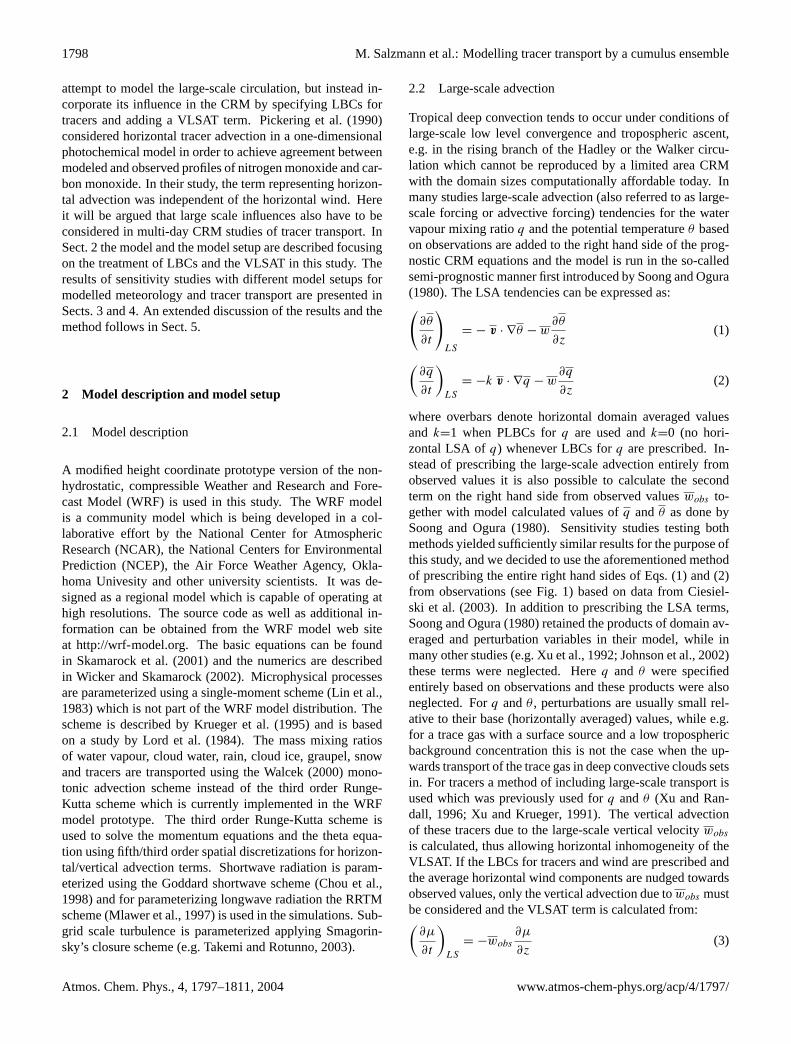
2.2 Large-scale advection

Tropical deep convection tends to occur under conditions oflarge-scale low level convergence and tropospheric ascent,e.g. in the rising branch of the Hadley or the Walker circu-lation which cannot be reproduced by a limited area CRMwith the domain sizes computationally affordable today. Inmany studies large-scale advection (also referred to as large-scale forcing or advective forcing) tendencies for the watervapour mixing ratioq and the potential temperatureθ basedon observations are added to the right hand side of the prog-nostic CRM equations and the model is run in the so-calledsemi-prognostic manner first introduced by Soong and Ogura(1980). The LSA tendencies can be expressed as:(

∂θ

∂t

)LS

= − v · ∇θ − w∂θ

∂z(1)

(∂q

∂t

)LS

= −k v · ∇q − w∂q

∂z(2)

where overbars denote horizontal domain averaged valuesand k=1 when PLBCs forq are used andk=0 (no hori-zontal LSA ofq) whenever LBCs forq are prescribed. In-stead of prescribing the large-scale advection entirely fromobserved values it is also possible to calculate the secondterm on the right hand side from observed valueswobs to-gether with model calculated values ofq andθ as done bySoong and Ogura (1980). Sensitivity studies testing bothmethods yielded sufficiently similar results for the purpose ofthis study, and we decided to use the aforementioned methodof prescribing the entire right hand sides of Eqs. (1) and (2)from observations (see Fig. 1) based on data from Ciesiel-ski et al. (2003). In addition to prescribing the LSA terms,Soong and Ogura (1980) retained the products of domain av-eraged and perturbation variables in their model, while inmany other studies (e.g. Xu et al., 1992; Johnson et al., 2002)these terms were neglected. Hereq and θ were specifiedentirely based on observations and these products were alsoneglected. Forq andθ , perturbations are usually small rel-ative to their base (horizontally averaged) values, while e.g.for a trace gas with a surface source and a low troposphericbackground concentration this is not the case when the up-wards transport of the trace gas in deep convective clouds setsin. For tracers a method of including large-scale transport isused which was previously used forq andθ (Xu and Ran-dall, 1996; Xu and Krueger, 1991). The vertical advectionof these tracers due to the large-scale vertical velocitywobs

is calculated, thus allowing horizontal inhomogeneity of theVLSAT. If the LBCs for tracers and wind are prescribed andthe average horizontal wind components are nudged towardsobserved values, only the vertical advection due towobs mustbe considered and the VLSAT term is calculated from:(

∂µ

∂t

)LS

= −wobs

∂µ

∂z(3)

Atmos. Chem. Phys., 4, 1797–1811, 2004 www.atmos-chem-phys.org/acp/4/1797/

M. Salzmann et al.: Modelling tracer transport by a cumulus ensemble 1799

Fig. 1. Time-height contour plots showing observed vertical and horizontal large-scale advection tendencies of potential temperature andwater vapour mixing ratio. Times are given in UTC.

www.atmos-chem-phys.org/acp/4/1797/ Atmos. Chem. Phys., 4, 1797–1811, 2004


whereµ is the modelled tracer mixing ratio andwobs is de-picted in Fig. 2c. Ifµ were inserted in Eq. (3) instead ofµ the tracer advection bywobs would be non-local and thetracer would be spuriously dispersed across the entire modeldomain. In addition it would become necessary to apply anon-local scaling of the values in order to ensure positivedefiniteness and mass conservation simultaneously. In sim-ulations of chemically reactive trace gases this would oftencause significant problems. The average horizontal wind isnudged towards observed values (see Fig. 2):(

∂v

∂t

)LS

= −v − vobs

τadj

(4)

wherev=(u, v), as in e.g. Xu and Randall (1996) and John-son et al. (2002) with an adjustment timeτadj=1 h.

2.3 Lateral boundary conditions

In semi-prognostic model studies of deep convection PLBCsare used and LSA terms for water vapour and potential tem-perature are prescribed providing a means of simulating ob-served events. With PLBCs no fluxes into the model domainfrom the outside are allowed and the domain averaged netupward transport of air is zero. While forq andθ the hori-zontal LSA terms (see Fig. 1b and d) can be small comparedto the vertical LSA terms (in Fig. 1a and c), this can not beexpected to be the case for moderately long lived trace gases,as will be demonstrated in this study. Thus, if no horizon-tal LSA terms for tracers are prescribed in multi-day studiesof trace gas transport, PLBCs should not be used for tracerswith lifetimes longer than those discussed above. Therefore,we decided to retain PLBCs for the potential temperature andthe air density but specify LBCs for tracers and for watervapour. In this approach, periodic boundary conditions arealso retained for the horizontal wind components, butu andv are nudged towards their observed values with extremelyshort adjustment times (twice the model timestepdt) at thelateral boundaries. Consequently, the LBCs foru andv canbe considered prescribed LBCs. The vertical velocityw andthe concentrations of all hydrometeors in the liquid and theice phase are set to zero at the lateral boundaries. The val-ues forq and the tracer concentration (partial densityµρ)at the lateral boundaries are specified in a zone which waschosen to be 2 grid points wide. Foru, v andw this widthis set to three points and additionally a four point wide re-laxation zone is used in which the adjustment time increaseslinearly in order to avoid the generation of spurious waves.The microphysics scheme is not applied in an eight-points-wide boundary zone in order to avoid spurious condensa-tion. This boundary zone is not considered in the analysisof the model results and not included in the domain lengthscited below. With the choice of LBCs presented here, tracersand water vapour are transported smoothly into the domainat the upstream lateral boundary. At the outflow boundarythe same boundary condition was applied. If a higher or-

der advection scheme were used, spurious upwind transportwould in principle be possible and a more sophisticated out-flow boundary condition may become necessary. In the runsusing specified lateral boundary conditions for water vapour,time-dependent water vapour boundary values were specifiedbased on observation-derived data from the Ciesielski et al.(2003) dataset.

2.4 Simulation of the TOGA-COARE case

A seven day period from 19–26 December 1992 at the siteof the TOGA COARE (Webster and Lukas, 1992) IntensiveFlux Array (IFA, centered at 2◦ S, 156◦ E) is modelled whichoverlaps with the period chosen by the GEWEX Cloud Sys-tem Study (GCSS Science Team, 1993) Working Group 4 asthe 2nd case of their first cloud-resolving model intercom-parison project (Krueger and Lazarus, 1999) and was alsoinvestigated by Wu et al. (1998), Andronache et al. (1999),Su et al. (1999), Johnson et al. (2002) and used in a modelcomparison by Gregory and Guichard (2001). During thisperiod the IFA region is influenced by the onset of a west-erly wind burst (see Fig. 2a) and three consecutive convectionmaxima develop between 20 and 23 December and a fourthand strongest maximum with its peak on 24 December at thetimes of maximum large-scale ascent (Fig. 2c) and verticalq andθ LSA (Fig. 1a and c). The WRF-model as describedin Sect. 2.1 is run with 2 km horizontal resolution and 350 mvertical resolution up to 19 km and decreasing resolution upto the model top at nearly 24.7 km with a total of 63 gridpoints in the vertical direction. The timestep is 5 s and smalltime varying random contributions (in the range±0.01 g/kgfor 2-D runs and±0.0125 g/kg for the 3-D run) are added tothe water vapour mixing ratio in the sub-cloud layer duringthe first 2.5 h of the simulation. Ten tracers with horizon-tally and vertically constant initial concentrations in 1750 mthick horizontal layers are included in the model runs. Forthree of these tracers a detailed analysis of the model resultswill be presented in the following. The tracers are assumedto be chemically inert, insoluble and to have no surface ortropospheric sources or sinks in the domain. At the lateralboundaries, the tracer concentrations are assumed to be con-stant and equal to their initial concentrations.

2.5 Sensitivity studies

The results from three 2-D runs, using a domain length of500 km are discussed in detail. These three runs were per-formed in order to study the sensitivity towards differentLBC and towards applying VLSAT. In the first run PLBCsare used. In the second run the water vapour, the concentra-tions of the hydrometeors in the liquid and the ice phase andthe wind are specified at the lateral boundaries as described inSect. 2.3. The tracer concentrations prescribed at the lateralboundaries are kept constant and are set equal to the initialtracer mixing ratios. For brevity, runs with specified tracer



Fig. 2. Time-height contour plots of observed(a) zonal(b) meridional and(c) vertical wind components.

Table 1. Sensitivity runs, for abbreviations see text.

Setup Boundary Conditions Large Scale Advection

2-D sensitivity runs

2-D (500 km) PLBC horiz. and vert.q, θ

2-D (500 km) SLBC vert.q, θ

2-D (500 km) SLBC vert.q, θ , and TLSA

3-D vs. 2-D sensitivity runs

2-D (248 km) SLBC vert.q, θ , and TLSA3-D (248 km×248 km) SLBC vert.q, θ , and TLSA

additional sensitivity runs

2-D (1000 km) SLBC vert.q, θ , and TLSA2-D (500 km), WRF Lin-scheme SLBC vert.q, θ ,and TLSA

and water vapour boundary conditions subsequently will bereferred to as specified lateral boundary condition (SLBC)runs. In the third run the LBCs (and the calculated meteo-rology) are the same as in the second run, but additionallya VLSAT term (Eq. 3) is added when solving the tracers’continuity equations. In order to study the dependence ofthe model results on the domain size, two additional model

runs using domain lengths of 248 km and 1000 km were per-formed. The results from these runs are mentioned occa-sionally and are not discussed in detail here. Except for thedifference in domain size, the setup of these runs was identi-cal to the setup of the third 500 km domain run, i.e. SLBCswere used and the VLSAT was considered. In Sect. 3, re-sults from an additional 2-D run are mentioned. The setup



Fig. 3. Time series of observed and modelled 6 h averaged surfaceprecipitation rates for PLBCs and for specified water vapour andwind LBCs.

of this run was identical to the third 500 km domain lengthrun, but instead of the single-moment microphysics schemedescribed in Sect. 2.1, the Lin-scheme implemented in thestandard WRF model was used. In addition to the 2-D runsdescribed above, a 3-D run was performed. In this run, againSLBCs were applied and the TLSA was considered. Thesame vertical grid configuration was used as in the 2-D runsand the horizontal domain size was 248 km×248 km. The re-sults of the 3-D run are compared to results from the 248 km2-D run. An overview over the different setups used in thesensitivity runs is presented in Table 1.

3 Modelled meteorology

The model computed precipitation rates generally comparewell with the observed data (see Fig. 3). The total observedamount of rain for the seven day period from 19–26 Decem-ber 1992 is calculated from the Ciesielski et al. (2003) datato be 149.1 mm and the simulated amount is 152.2 mm forthe run with PLBCs. In SLBC runs the values are 162.6 mmfor the 2-D and 171.8 mm for the 3-D run and thus some-what higher than the observed value. On the other hand ina comparable 2-D run also using SLBCs but the Lin-schemefrom WRF instead of the one described in Sect. 2.1, the com-puted value is 143.7 mm and is thus somewhat lower than theobserved value (not shown in the figure). In general, withPLBCs a large over- or underestimation is unlikely to oc-cur in a semi-prognostic setup since the computed amount ofsurface precipitation is largely constrained by the input datafor the water vapour LSA. In contrast, with SLBCs the do-main averaged horizontal flux divergence for water vapourat a given height level is determined by the model and is al-lowed to deviate from the measured values of the horizontalLSA, thus more easily allowing either an over- or an under-estimation of the surface precipitation.

Fig. 4. Vertical profiles of observed and modelled domain and timeaveraged temperatures and water vapour mixing ratios.

Figure 4 depicts the differences between model calculatedand observed average temperatures and water vapour mixingratios. The cold temperature bias in the model runs in thetroposphere is comparable to the bias in the 2-D-CRM studyof Johnson et al. (2002) and for the 3-D run to the bias inthe 3-D CRM model study of Su et al. (1999). The cold biaswas e.g. discussed by Johnson et al. (2002). The differentq biases in the SLBC runs compared to the PLBC runs area consequence of the horizontal transport of water vapourinto the domain, and of the differences in total precipitationdiscussed above.

For the 500 km domain 2-D runs the Hovmoller diagramsin Fig. 5a and b show squall lines propagating westwards atmoderate speeds of mostly∼3 m/s (low propagation speedimplies a steep slope in the diagrams) and faster eastwardsmoving single clouds (thin “lines” in the diagrams) for bothPLBCs and SLBCs.



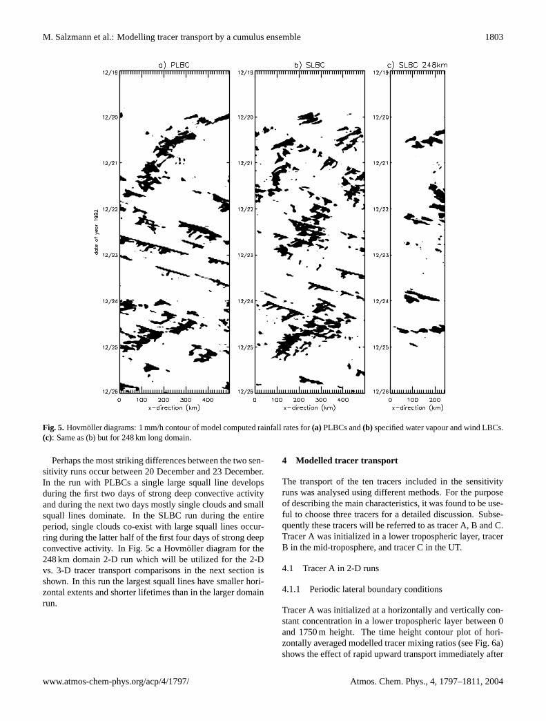
Fig. 5. Hovmoller diagrams: 1 mm/h contour of model computed rainfall rates for(a) PLBCs and(b) specified water vapour and wind LBCs.(c): Same as (b) but for 248 km long domain.

Perhaps the most striking differences between the two sen-sitivity runs occur between 20 December and 23 December.In the run with PLBCs a single large squall line developsduring the first two days of strong deep convective activityand during the next two days mostly single clouds and smallsquall lines dominate. In the SLBC run during the entireperiod, single clouds co-exist with large squall lines occur-ring during the latter half of the first four days of strong deepconvective activity. In Fig. 5c a Hovmoller diagram for the248 km domain 2-D run which will be utilized for the 2-Dvs. 3-D tracer transport comparisons in the next section isshown. In this run the largest squall lines have smaller hori-zontal extents and shorter lifetimes than in the larger domainrun.

4 Modelled tracer transport

The transport of the ten tracers included in the sensitivityruns was analysed using different methods. For the purposeof describing the main characteristics, it was found to be use-ful to choose three tracers for a detailed discussion. Subse-quently these tracers will be referred to as tracer A, B and C.Tracer A was initialized in a lower tropospheric layer, tracerB in the mid-troposphere, and tracer C in the UT.

4.1 Tracer A in 2-D runs

4.1.1 Periodic lateral boundary conditions

Tracer A was initialized at a horizontally and vertically con-stant concentration in a lower tropospheric layer between 0and 1750 m height. The time height contour plot of hori-zontally averaged modelled tracer mixing ratios (see Fig. 6a)shows the effect of rapid upward transport immediately after



Fig. 6. 2-D sensitivity runs: Time-height contour plots of domainaveraged tracer mixing ratios for tracer A initialized at a horizon-tally and vertically constant concentration in a layer between 0 and1750 m altitude. The mixing ratio values plotted in this figure arenormalized to the maximum initial mixing ratio.(a) Periodic lateralboundary conditions,(b) specified water vapour and wind lateralboundary conditions,(c) specified lateral boundary conditions andvertical large scale advection for tracers. Contour levels are: 0.0,0.02, 0.05, 0.1, 0.15, 0.2, 0.25, 0.3, 0.4, 0.5, 0.6, 0.7, 0.8, 0.9. and1.0.

the onset of modelled deep convection at∼23 UTC on 19December. Within the next day the amount of tracer in theboundary layer decreases rapidly, while in the UT a localmaximum of the tracer mixing ratio forms (at the height ofthe cloud anvils). The altitude of this maximum starts de-creasing immediately because of tracer mass descending dueto the mass balancing mesoscale subsidence induced by thedeep convection. Furthermore the mixing ratio of the tracerclose to the surface is sufficiently depleted so that air ad-vected rapidly upwards would not contain high enough tracermixing ratios to account for the formation of further UT mix-ing ratio maxima. Later the vertical mixing is increased sincesome of the descending tracer is re-entrained into deep con-vective clouds and transported upwards. Four days after theonset of deep convection the tracer is well mixed throughoutthe model troposphere.

4.1.2 Specified lateral boundary conditions

As previously mentioned specifying LBCs for tracer allowsfor tracer advection across the model’s lateral boundariesand the total amount of tracer inside the domain to be in-fluenced by the mean horizontal wind. Like in the case ofPLBCs tracer mass is rapidly transported from the lower tro-posphere (LT) to the UT when deep convection sets in (see

Fig. 6b). Initially the LT mixing ratio decreases as in thecase of PLBCs. But between 21 December and 22 Decem-ber the westerly wind burst sets in and wind speeds in theLT increase (see Fig. 2a). Tracer mass transported awayfrom the LT inside the updrafts of the deep convective cloudsis replenished by tracer mass horizontally advected into themodel domain. Around the same time the wind increases inthe UT and tracer mass is continously advected out of thedomain across the lateral boundaries. The amount of traceradvected into the domain in the LT and the amount of trac-ers advected out of the domain at UT levels could be quan-titatively assessed calculating the time-integrated horizontaland vertical advection tendencies. Integrated over longerepisodes, the tendencies of horizontal and vertical advectionat each vertical level approximately balance. As for the runwith PLBCs (Fig. 6a), UT mixing ratio maxima with con-tours sloping towards the Earth’s surface indicate the strongeffect of mesoscale subsidence. When the VLSAT term istaken into account (see Fig. 6c) this effect of the mesoscalesubsidence is also visible particularly at the time of the max-imum in convective activity on 24 December, but once in-jected into the UT, the tracer mass often remains there forconsiderably longer times. For tracer A domain averagedvertical profiles are plotted in Fig. 7 reflecting the differencesbetween the results of the different sensitivity runs discussedhere. Significant differences between the SLBC run and therun with PLBCs already become apparent in Fig. 7b (lessthan 24 h after the onset of deep convection in the model).The profiles in Fig. 7 will be discussed in more detail inSect. 5.

4.2 Tracer B in 2-D runs


Tracer B (see Fig. 8a) was initialized at a constant concentra-tion in a layer between 7000 and 8750 m height and is chosenas a representative mid-tropospheric tracer. At the onset ofdeep convection this tracer is less effectively transported up-wards since the levels of maximum entrainment of deep con-vective clouds are located in the lower troposphere (LT). Theamount of tracer B in the UT increases much less rapidly thanthat of tracer A (compare Fig. 8a to Fig. 6a), because tracerB is less efficiently entrained into deep convective cells thantracer A. The finding that tracer B is entrained less efficientlythan tracer A and that tracer A is predominantly detrained inthe UT provides a different perspective than the “convectiveladder” effect postulated by Mari et al. (2000). Tracer B isalso transported downwards due to the mesoscale subsidenceand after two days of active deep convection a substantialpart of it has reached the LT from where it is then rapidlytransported upwards. At the end of the studied period thistracer is still not homogeneously distributed throughout theentire troposphere.



Fig. 7. Domain averaged vertical tracer profiles for tracer A every 12 h after the modelled convection sets in for a run with PLBCs (dottedline), a run in which the tracer concentrations were specified at the lateral domain boundary (dashed line) and a run with specified LBCs andVLSAT (solid line). Mixing ratio values were normalized to the maximum initial mixing ratio.


During the first two days of the model run, the domain aver-aged mixing ratio for tracer B evolves similarly to its counter-part in the run with PLBCs when the VLSAT term is omitted(see Fig. 8b). When the VLSAT term is incorporated (seeFig. 8c) the mesoscale downward transport on 20 Decemberis largely compensated. In Fig. 9 the mixing ratio contoursof tracer B on 20 December 14:00 GMT are depicted for thethree different sensitivity runs. In the run with PLBCs themesoscale subsidence has caused the center of tracer mass tosubside to nearly 3 km below its initial location. The strong

effect of the mesoscale subsidence is also apparent for theSLBC run in Fig. 9b where the mixing ratio contours slopedownwards from the inflow toward the outflow boundary. Inthe run in which the VLSAT term was included on the otherhand a large fraction of the tracer mass has remained at itsinitial height. Between 21 and 22 December (see Fig. 8bagain) when the westerly wind burst sets in, the total amountof tracer B in the domain decreases as a consequence ofmesoscale subsidence, wind shear and transport across thelateral domain boundary. First the tracer is transported down-wards because of the mesoscale subsidence to altitudes be-low 5 km where the average westerly wind is strong. From



Fig. 8. As Fig. 6 for tracer B initialized at a constant concentrationbetween 7000 and 8750 m.

Fig. 9. Tracer B: X-Z contour plot of the normalized mixing ratio∼16 h after the onset of modelled convection. The contour intervalis 0.1. Dashed lines indicate the initial tracer location, the solidline is the 0.1 g/kg mixing ratio contour of the sum of all masses ofhydrometeors in the ice and the liquid phase.

there it is rapidly transported eastwards to where it leavesthe domain across its lateral boundary. For the tracer in theVLSAT run, in total more tracer mass remains inside the do-main because the transport due to the mesoscale subsidenceis largely compensated by the VLSAT. Around 24 December

Fig. 10.As Fig. 6 for tracer C initialized at a constant concentrationbetween 12 250 and 14 000 m.

the easterly wind at above 5 km height reaches a local maxi-mum which transports “fresh” tracer into the domain. For asmaller domain (e.g. 248 km, see Fig. 12a) the depletion ofthe tracer mass in the domain is weaker because during thetime τadv it takes the tracer to be advected across the entirelength of the domain a smaller fraction of the tracer mass istransported downwards due to the mesoscale subsidence. Fora larger model domain (1000 km) the depletion is also weaker(figure not shown) becauseτadv is long enough so that not allof the tracer transported downward is transported out of thedomain during the period before tracer mass is replenishedby the increasing easterly wind.

4.3 Tracer C in 2-D runs


Tracer C (see Fig. 10a) was initialized in an upper tropo-spheric layer between 12 250 and 14 000 m. About 12 h afterthe onset of the deep convection the first convection towerspenetrate this layer and initiate downwards transport. Theair inside the anvils carries a low tracer mixing ratio andreplaces the air with high mixing ratios in the UT (whichis pushed downwards along the lower edge of the anvils).Mesoscale subsidence acts to further transport tracer masstowards the Earth’s surface. On 22 December a reduction indomain averaged mixing ratio located at∼10 km altitude iscalculated. The decrease in mixing ratio leading to this min-imum is attributed to the transport of air with a low tracermixing ratio from the LT to the UT. At the time of the subse-quent increase of mixing ratio in the UT some air containinghigh tracer mixing ratio has reached the LT from where itis again transported upwards inside deep convective clouds.



Fig. 11. As Fig. 6 but(a) for the 248 km long 2-D domain and(b)for the 248 km×248 km horizontal area 3-D domain.

Four days after the onset of deep convection the tracer isfairly well mixed throughout most of the model troposphere.


As for the run with PLBCs tracer C is influenced by the pen-etration of deep convective towers and by mesoscale subsi-dence (see Fig. 10b and c). Because of the UT easterly windssome of the tracer mass advected downwards is replenishedfrom outside the domain. If VLSAT is taken into accountin the model (see Fig. 10c) considerably less tracer mass istransported to the LT than for the run with VLSAT switchedoff (Fig. 10b).

4.4 Comparison 2-D vs. 3-D model runs

Here, tracer transport results from a 3-D run with a248 km×248 km horizontal domain size are compared to re-sults from a 2-D run with a 248 km long domain. As de-scribed in Sect. 2.5 both runs were performed using SLBCsfor the tracers and taking into account the VLSAT term. Fortracer A, the results from both runs are depicted in Fig. 11.The time-height contours of the domain averaged tracer mix-ing ratio are smoother for the 3-D run than for the 2-D run,but the main features in Fig. 11a and b are similar, particu-larly during the first two days of active deep convection whenthe meridional wind component (see Fig. 2b) is small. On22 December the southerly wind component in the UT startsincreasing as well as the northerly wind component in themid-troposphere. In the mid-troposhere tracer mass is ad-vected out of the 3-D domain across the southern boundaryon the 23rd (compare Fig. 11b). On 25 December an increas-ing southerly wind component in the mid-troposphere leadsto an increase of tracer advection out of the domain acrossthe northern boundary which is reflected in the t-z contourplot for the 3-D run. For tracer B (see Fig. 12) one difference

Fig. 12.As Fig. 11 for a tracer initialized at a constant concentrationbetween 7000 and 8750 m.

is the amount of tracer that remains in the lower troposphere.In the 3-D run, meridional tracer transport in the layers belowthe initial tracer mass location acts to advect tracer mass outof the domain. Cross-boundary advection in the meridionaldirection is also found to play an important role for the differ-ences of the domain averaged mixing ratios of tracer C (seeFig. 13). Again subsiding tracer mass is advected out of thedomain in the 3-D run due to the non-zero meridional windcomponent, while in the 2-D run advection in the meridionaldirection is not considered. Figure 14 shows the maximumcloud top heights in the domain for different runs. The cloudtop height was defined as the first model level where thesum of all cloud meteor masses integrated downwards start-ing from the model top exceeds 5·10−3kg/m2. Most notably,the maximum cloud top heights for the 3-D run are generallyabove those for the corresponding 2-D run. For the 500kmdomain 2-D runs, the maximum cloud top heights are largelyindependent of the boundary conditions applied. Differencesin the downwards transport of tracer C are most likely causedby the application of VLSAT rather than by systematicallydifferent cloud top heights. Differences between 2-D and3-D tracer transport model runs can also arise due to dynam-ical or microphysical reasons (e.g. Wang and Prinn, 2000).This study focuses mainly on the differences due to crossboundary transport. Cross boundary transport is believed tobe the main reason for the differences between the results ofthe 2-D and the 3-D run presented here, but further research,including a 3-D simulation with PLBC, is needed in order tobetter differentiate between the different processes involved.

5 Discussion

Many trace gas compounds with tropospheric lifetimes be-tween a few hours and a few weeks such as carbon monoxideor NOx (nitric oxide + nitrogen dioxide) have a source close



Fig. 13.As Fig. 11 for a tracer initialized at a constant concentrationbetween 12 250 and 14 000 m.

to the Earth’s surface. Measured vertical mixing ratio pro-files of these compounds in the vicinity of deep convectionare often “C”- shaped, i.e. have a maximum in the LT anda second maximum in the UT (e.g. Dickerson et al., 1987;Gidel, 1983). On the other hand in post convective environ-ments profiles of trace gases with a sink in the LT often havea minimum in the LT and a second minimum in the UT (e.g.Kley et al., 1997). Sometimes such a profile is referred to as“D”-shaped.

Tracer A can be considered an idealization of a moderatelylong lived, insoluble trace gas with a surface source. Its ini-tial profile represents its idealized profile in an environmentwhich has not been influenced by (either local or remote)deep convection recently. Figure 7 shows vertical profiles ofmodel calculated tracer profiles for this tracer. During thefirst 36 h the tracer profile in the run with PLBCs still dis-plays the typical “C”-shape caused by intermittent deep con-vective transport. After roughly three days the tracer is wellmixed. If a constant wind speed of 5 m/s is assumed, threedays would correspond to a horizontal transport distance of∼1300 km which is still smaller than the entire Pacific WarmPool suggesting that moderately long lived tracers would bewell mixed after having been advected at this wind speedstraight across the entire Pacific Warm Pool. This could pos-sibly also be expected as a result in a tracer CRM study withSLBCs and a sufficiently large domain size.

If chemistry transport CRM results are to be compared tomeasurements from field campaigns covering a limited area,a multi-day simulation with PLBCs will probably be of lim-ited use since for moderately long lived tracers the effect ofhorizontal advection on these time scales is not negligibleas demonstrated by the differences in Fig. 7b to f and dis-cussed previously. On the other hand, if LBCs would bespecified from measurements, the method presented in thisstudy could in principle be used for CRM simulations of

Fig. 14. Domain maximum cloud top heights. The sampling timewas 30 min and a 3 h moving average is plotted. The cloud topheight was defined as the first model level where the sum of allcloud meteor masses integrated downwards starting from the modeltop exceeds 5·10−3kg/m2.

trace gas dispersion due to deep convective clouds. How-ever, in order to obtain the necessary input data for such asimulation, a comprehensive field campaign of the size of theTOGA-COARE campaign encompassing both meteorologi-cal and trace gas measurements would be necessary. No suchcampaign has been planned. Nevertheless, input data fromdifferent sources, including both field campaigns and resultsfrom global chemistry transport models (GCTMs) could beused to specify the necessary boundary conditions for CRMswith the setup proposed here.

Here the transport of idealized tracers was studied and theboundary conditions were kept fixed. For more realistic stud-ies, time-dependent boundary values for trace gases can beprescribed to the extent they are available.

Another potentially useful application for the setup de-scribed in this study could be the comparison between tracertransport results from CRMs and parameterizations used inglobal models. In global chemistry transport models con-vective transport constitutes a major source of uncertaintysince it is highly sensitive to the convective parameteriza-tion applied (Mahowald et al., 1995) and even to the treat-ment of transport based on the mass fluxes provided by in-dividual schemes (Lawrence and Rasch, submitted, 2004)1.Cloud-resolving models (CRMs) in combination with singlecolumn models (SCMs) could perhaps help to better evalu-ate these parameterizations and thus reduce this uncertainty.For TOGA-COARE a comparison between different singlecolumn models including tracer transport was presented byRasch et al. (2003). A similar framework as the one pre-sented here could be used in multi-day single column model

1Lawrence, M. G. and Rasch, P. J.: Tracer transport in deepconvective updrafts: plume ensemble versus bulk formulations, J.Atmos. Sci., submitted, 2004.



(SCM) studies. Comparisons between SCMs and CRMswould draw substantial benefits from the method presentedhere. In current global models convective tracer transport iscommonly parameterized using the assumption that the up-wards advection of air mass inside the convective clouds isbalanced by the mesoscale subsidence in the same verticalmodel column. The tracer transport due to large-scale ascentis calculated separately using the so-called operator splittingtechnique. This method used in global models is analogousto the method used here, in this CRM study.

The setup with specified LBCs for water vapour allowsfor larger differences between modelled and observed sur-face precipitation than the setup with PLBCs and thus couldpossibly be useful for evaluating different microphysicsschemes.

A drawback of specifying LBCs for tracers and retainingPLBCs for the air density is that the advection of tracer massat a given height level due to the domain averaged horizontalair mass convergence or divergence into or out of the domainis neglected. The domain averaged mass flux divergence (ad-vection) of the tracers is due to the difference in influx andoutflux across the domain boundaries in this study. While thetracer mass flux at the inflow boundary depends on the spec-ified tracer concentration and the wind, the mass flux at theoutflow boundary is influenced by the modelled tracer trans-port inside the domain. In small domains containing a singleconvective system and under conditions of weak horizontalaverage winds, the domain averaged mass flux divergencedue to large scale wind convergence and divergence into andout of the model domain is likely to become important.

The results of runs using SLBCs for tracers are domainsize dependent, although in this study the differences be-tween the runs with 500 km domain size (see Figs. 6c to10c) and 248 km domain size (see Figs. 11c to 13c) are oftensmall. For either much smaller or much larger domains, astronger domain size dependence may be expected. This do-main size dependence should not be considered a drawbackof the method but is an advantage in cases in which model re-sults from future multi-day chemistry transport CRM studiesare to be compared to measurements.

In the case study presented here, the VLSAT often has astrong effect on the domain averaged vertical profiles, partic-ularly whenτadv is long (e.g. Fig. 7e–g, k, and l) and shouldnot be neglected. In CRM studies of reactive tracer transportthe over-estimation of downwards trace gas transport, as seenin tracers B and C, could otherwise for example lead to unre-alistically high chemical NOx sources in the mid-tropospheredue to the thermal decomposition of subsiding PAN (per-oxy acetyl nitrate) or pernitric acid. The spurious downwardtransport of tracers when the VLSAT is neglected can easilybe mis-interpreted as the effect of mid-level detrainment.

The results for the PLBC runs in this study are similar tothe results presented by Lu et al. (2000), i.e., in the modelruns with PLBC, the tracers are transported from the mid-and upper troposphere to the LT with a timescale of approx-

imately one day. Figures 15 and 16 of Lu et al. (2000) canbe compared to Figs. 6a to 10a for the first days of modelleddeep convection. Lu et al. (2000) chose to re-initialize theirmodel every 60 h and used a domain length of 512 km. Usingsensitivity runs for a 500 km domain, it was demonstrated inthis study that the modelled tracer transport is highly sensi-tive to the choice of LBC, even on timescales of a few days.Furthermore it was shown that including VLSAT changessome main characteristics of the modeled tracer transport.In multi-day CRM studies of tracer transport in regions withlarge scale vertical ascent, such as the Pacific Warm Pool, theVLSAT term has to be considered. Since current CRMs donot allow the exchange of airmass across the lateral domainboundaries, the VLSAT must be considered as well as thecorresponding terms forq andθ .

6 Conclusions

A setup designed for modelling multi-day tracer transport ina current CRM was described and the transport of idealizedtracers was studied. The results obtained with this setup werecompared to results obtained with a setup previously usedin a similar case study (Lu et al., 2000). In the new setup,specifying LBCs for tracers allows the effects of horizontaltracer advection into and out of the model domain to be con-sidered. Less than 24 h after the onset of deep convectionin the model, the results for the different setups started todiffer significantly. In general, if no large scale advectionterms for tracers are prescribed from observations, PLBCsshould not be used for model studies of tracer transport if thesimulated timetsim is longer than the advective time scaleτadv=L/vmax andτl>τadv, whereτl is the tracer’s chemicallife time. For studies of reactive, or soluble tracer transport,prescribing horizontally homogeneous horizontal tracer LSAterms from observations could in some cases be problematicbecause large horizontal gradients can form in the simula-tions. This would have to be examined in future studies.

Furthermore it was demonstrated that including a VLSATterm, which was not included in previous studies of tracertransport, partially compensates the net-downward transportof tracers from the middle and upper troposphere due to themesoscale subsidence induced by deep convection. This termshould be considered in future multi-day limited area CRMstudies of tracer transport.

For the first time, tracer transport results from a multi-day 3-D model run were presented and compared to resultsfrom a 2-D run. Differences between the 2-D and 3-D runwere mainly attributed to an increase in horizontal advectionacross the lateral domain boundaries due to the meridionalwind component in the 3-D model runs which was not con-sidered in the 2-D simulations.

The model setup used in this study facilitates comparisonswith either trace gas measurements from multi-day field cam-paigns or with results from single column cloud models, thus



possibly providing one means to help evaluate deep convec-tive transport parameterizations used in global models.

A drawback of the new setup arises from retaining PLBCsfor air density. In the future a model setup allowing the con-vergence or divergence of airmass into or out of the modeldomain at a given height could be considered for trace gastransport studies. One possibility would be to try to de-velop a method using nested models in combination withe.g. a gridded input dataset based on meteorological mea-surements from the TOGA-COARE campaign. In contrastto conventional CRMs, the WRF model was designed as aregional model which is capable of operating at high resolu-tions. WRF allows for multiple nesting, and air quality mod-els based on WRF are currently being developed at differentinstitutions including NCAR.

The setup as described here will be used to investigatethe effect of a cumulus ensemble on the dispersion of re-active trace gases such as ozone. For this purpose a tropo-spheric chemistry mechanism based on the global Model ofAtmospheric Transport and Chemistry – Max Planck Insti-tute for Chemistry (MATCH-MPIC, Lawrence et al., 1999;von Kuhlmann et al., 2003, and references therein) has beenimplemented into the CRM. Furthermore, a more compre-hensive study about the sensitivity of the tracer transport re-sults to different model configurations such as different reso-lutions, microphysics schemes and domain sizes is planned.

Acknowledgements.We appreciate valuable discussions withseveral colleagues, especially R. von Kuhlmann and B. Bonn, andvaluable comments by C. Wang and two other anonymous referees.This research was supported by funding from the German Ministryof Education and Research (BMBF), project 07-ATC-02. Resultsfrom this study will be submitted in a Ph.D. thesis at the Universityof Mainz, Department for Atmospheric Physics.

Edited by: U. Lohmann

References

Andronache, C., Donner, L. J., Seman, C. J. Ramaswamy, V., andHemler, R. S., : Sulfur dioxide in remote oceanic air: Atmo-spheric sulfur and deep convective clouds in tropical Pacific: Amodel study, J. Geophys. Res., 104, 4005–4024, 1999.

Chatfield, R. B. and Crutzen, P. J.: Sulfur dioxide in remote oceanicair: Cloud transport of reactive precursors, J. Geophys. Res., 89,7111–7132, 1984.

Chou, M.-D., Suarez, M. J., Ho, C.-H., Yan, M. M.-H., and Lee,K.-T.: Parameterizations for cloud overlapping and shortwavesingle-scattering properties for use in general circulation andcloud ensemble models, J. Climate, 11, 202–214, 1998.

Ciesielski, P. E., Johnson, R. H., Haertel, P. T., and Wang, J.: Cor-rected TOGA COARE sounding humidity data: Impact on diag-nosed properties of convection and climate over the warm pool,J. Climate, 16, 2370–2384, 2003.

Dickerson, R. R., Huffman, G. J., Luke, W. T., Nunnermacker, L. J.,Pickering, K. E., Leslie, A. C. D., Lindsey, C. G., Slinn, W. G. N.,

Kelly, T. J., Daum, P. H., Delaney, A. C., Greenberg, J. P., Zim-merman, P. R., Boatman, J. F., Ray, J. D., and Stedman, D. H.:Thunderstorms: An important mechanism in the transport of airpollutants, Science, 235, 460–465, 1987.

Ekman, A. M. L., Wang, C., Strom, J., and J. Wilson: Explicit sim-ulation of aerosol physics in a cloud-resolving model, Atmos.Chem. Phys., 4, 773–791, 2004,SRef-ID: 1680-7324/acp/2004-4-773.

GCSS Science Team: The GEWEX Cloud System Study (GCSS),Bull. Am. Met. Soc., 74, 387–399, 1993.

Gidel, L. T.: Cumulus cloud transport of transient tracers, J. Geo-phys. Res., 88, 6587–6599, 1983.

Gregory, D. and Guichard, F.: Aspects of the parameterization oforganized convection: Contrasting cloud resolving model andsingle-column model realizations, Q. J. R. Meteorol. Soc., 128,625–646, 2001.

Johnson, D. E., Tao, W.-K., Simpson, J., and Sui, C.-H.: A studyof the response of deep tropical clouds to large-scale thermody-namic forcings, Part I: Modeling strategies and simulations ofTOGA COARE convective systems, J. Atmos. Sci., 59, 3492–3518, 2002.

Kley, D., Smit, H. G. J., Vomel, H., Grassl, H., Ramanathan, V.,Crutzen, P. J., Williams, S., Meyerwerk, J., and Oltmans, S. J.:Tropospheric water-vapour and ozone cross-sections in a zonalplane over the central equatorial Pacific Ocean, Q. J. R. Meteorol.Soc., 123, 2009–2040, 1997.

Krueger, S. K. and Lazarus, S. M.: Intercomparison of multi-daysimulations of convection during TOGA COARE with severalcloud-resolving and single-column models, in Preprints, 23rdConf. on Hurricanes and Tropical Meteorology, Amer. Meteor.Soc., Dallas, TX, 1999.

Krueger, S. K., Fu, Q., Liou, K. N., and Chin, H.-N. S.: Improve-ments of an ice-phase microphysics parameterization for use innumerical simulations of tropical convection, J. Appl. Met., 34,281–287, 1995.

Lawrence, M. G., Crutzen, P. J., Rasch, P. J., Eaton, B. E., andMahowald, N. M.: A model for studies of tropospheric photo-chemistry: Description, global distributions, and evaluation, J.Geophys. Res., 104, 26 245–26 277, 1999.

Lawrence, M. G., von Kuhlmann, R., Salzmann, M., and Rasch,P. J.: The balance of effects of deep convective mixing on tropo-spheric ozone, Geophys. Res. Lett., 30, art. no. 1940, 2003.

Lelieveld, J. and Crutzen, P. J.: Role of deep cloud convection inthe ozone budget of the troposphere, Science, 264, 1759–1761,1994.

Lin, Y.-L., Farley, R. D., and Orville, H. D.: Bulk parameterizationof the snow field in a cloud model, J. Climate Appl. Meteor., 2,1065–1092, 1983.

Lord, S. J., Willoughby, H. E., and Piotrowicz, J. M.: Role of a pa-rameterized ice-phase microphysics in an axisymmetric, nonhy-drostatic tropical cyclone model, J. Atmos. Sci., 42, 2836–2848,1984.

Lu, R., Lin, C., Turco, R., and Arakawa, A.: Cumulus transport ofchemical tracers, 1. Cloud-resolving model simulations, J. Geo-phys. Res., 105, 10 001–10 221, 2000.

Mahowald, N. M., Rasch, P. J., and Prinn, R. G.: Cumulus parame-terizations in chemical transport models, J. Geophys. Res., 100,26 173–26 189, 1995.



Mari, C., Jacob, D. J., and Bechtold, P.: Transport and scavengingof soluble gases in a deep convective cloud, J. Geophys. Res.,105, 22 255–22 267, 2000.

Mlawer, E. J., Taubman, S. J., Brown, P. D., Iacono, M. J., andClough, S. A.: Radiative transfer for inhomogeneous atmo-sphere: RRTM a validated correlated-k model for the longwave,J. Geophys. Res., 102, 16 663–16 682, 1997.

Pickering, K. E., Thompson, A. M., Dickerson, R. R., Luke, W. T.,McNamara, D. P., Greenberg, J. P., and Zimmerman, P. R.:Model calculations of tropospheric ozone production potentialfollowing observed convective events, J. Geophys. Res., 95,14 049–14 062, 1990.

Pickering, K. E., Thompson, A. M., Kim, H., DeCaria, A. J., Pfis-ter, L., Kucsera, T. L., Witte, J. C., Avery, M. A., Blake, D. R.,Crawford, J. H., Heikes, B. G., Sachse, G. W., Sandholm, S. T.,and Talbot, R. W.: Trace gas transport and scavenging in PEM-Tropics B South Pacific Convergence Zone convection, J. Geo-phys. Res., 106, 32 591–32 602, 2001.

Rasch, P., Zurovac-Jevtic, D., Emanuel, K., and Lawrence, M.:Consistent representation of convective processes for chemistryand climate models, Geophys. Res. Abstr., 5, 12 440, 2003.

Scala, J. R., Garstang, M., Tao, W.-K., Pickering, K. E., Thomp-son, A. M., Simpson, J., Kirchhoff, V. W. J. H., Browell, E. V.,Sachse, G. W., Torres, A. L., Gregory, G. L., Rasmussen, R., andKhalil, M. A. K.: Cloud draft structures and trace gas transport,J. Geophys. Res., 95, 17 015–17 030, 1990.

Skamarock, W. C., Klemp, J. B., and Dudhia, J.: Prototypes for theWRF (Weather Research and Forecasting) model, in Preprints,Ninth Conf. Mesoscale Processes, pp. J11–J15, Amer. Meteor.Soc., Fort Lauderdale, FL, 2001.

Skamarock, W. C., Powers, J. G., Barth, M., Dye, J. E., Mate-jka, T., Bartels, D., Baumann, K., Stith, J., Parrish, D. D., andHubler, G.: Numerical simulations of the July 10 Stratospheric-Tropospheric Experiment: Radiation, Aerosols, and Ozone/DeepConvection Experiment convective system: Kinematics andtransport, J. Geophys. Res., 105, 19 973–19 990, 2000.

Soong, S.-T. and Ogura, Y.: Response of tradewind cumuli to large-scale processes, J. Atmos. Sci., 37, 2035–2050, 1980.

Su, H., Chen, S. S., and Bretherton, C. S.: Three-dimensional week-long simulations of TOGA COARE convective systems using theMM5 mesoscale model, J. Atmos. Sci., 56, 2326–2344, 1999.

Takemi, T. and Rotunno, R.: The effects of subgrid model mixingand numerical filtering in simulations of mesoscale cloud sys-tems, Mon. Weather Rev., 131, 2085–2191, 2003.

von Kuhlmann, R., Lawrence, M. G., Crutzen, P. J., and Rasch,P. J.: A model for studies of tropospheric ozone and nonmethanehydrocarbons: Model description and ozone results, J. Geophys.Res., 108, doi:10.1029/2002JD002893, 2003.

Walcek, C. J.: Minor flux adjustment near mixing ratio extremesfor simplified yet highly accurate monotonic calculation of traceradvection, J. Geophys. Res., 105, 9335–9348, 2000.

Wang, C. and Chang, J. S.: A three-dimensional numerical model ofcloud dynamics, microphysics, and chemistry: 3. Redistributionof pollutants, J. Geophys. Res., 98, 16 787–16 798, 1993.

Wang, C. and Prinn, R. G.: On the roles of deep convective cloudsin tropospheric chemistry, J. Geophys. Res., 105, 22 269–22 297,2000.

Webster, P. J. and Lukas, R.: TOGA COARE: The Coupled Ocean-Atmosphere Response Experiment, Bull. Am. Met. Soc., 73,1377–1416, 1992.

Wicker, L. J. and Skamarock, W. C.: Time-splitting methods forelastic models using forward time schemes, Mon. Weather Rev.,130, 2088–2097, 2002.

Wu, X., Grabowski, W. W., and Moncrieff, M. W.: Long-term be-havior of cloud systems in TOGA COARE and their interactionswith radiative and surface processes. Part I: Two-dimensionalmodeling study, J. Atmos. Sci., 55, 2693–2714, 1998.

Xu, K.-M. and Krueger, S. K.: Evaluation of cloudiness parameter-izations using a cumulus ensemble model, Mon. Weather Rev.,119, 342–367, 1991.

Xu, K.-M. and Randall, D.: Explicit simulation of cumulus ensem-bles with GATE phase III data: Comparison with observations,J. Atmos. Sci., 53, 3710–3736, 1996.

Xu, K.-M., Arakawa, A., and Krueger, S. K.: The macroscopic be-haviour of cumulus ensembles simulated by a cumulus ensemblemodel, J. Atmos. Sci., 49, 2402–2420, 1992.


Documents

and Physics Modelling tracer transport by a cumulus ... Physics Modelling tracer transport by a cumulus ensemble: lateral boundary conditions and large-scale ascent M. Salzmann1, M