Japan Atomic Energy Agency

日本原子力研究開発機構機関リポジトリ Japan Atomic Energy Agency Institutional Repository

Title Evaluation of ambient dose equivalent rates influenced by vertical and horizontal distribution of radioactive cesium in soil in Fukushima Prefecture

Author(s) Malins A., Kurikami Hiroshi, Nakama Shigeo, Saito Tatsuo, Okumura Masahiko, Machida Masahiko, Kitamura Akihiro

Citation Journal of Environmental Radioactivity,151(1),p.38-49

Text Version Author's Post-print

URL https://jopss.jaea.go.jp/search/servlet/search?5050041

DOI https://doi.org/10.1016/j.jenvrad.2015.09.014

Right © <2016>. This manuscript version is made available under the CC-BY-NC-ND 4.0 license http://creativecommons.org/licenses/by-nc-nd/4.0/

Evaluation of ambient dose equivalent rates influenced by vertical andhorizontal distribution of radioactive cesium in soil in Fukushima Prefecture

Alex Malinsa,∗, Hiroshi Kurikamib, Shigeo Nakamac, Tatsuo Saitob, Masahiko Okumuraa, MasahikoMachidaa, Akihiro Kitamurab

aCenter for Computational Science & e-Systems, Japan Atomic Energy Agency, 178-4-4 Wakashiba, Kashiwa, Chiba,277-0871, Japan

bSector of Fukushima Research and Development, Japan Atomic Energy Agency, 4-33 Muramatsu, Tokai-mura, Naka-gun,Ibaraki, 319-1194, Japan

cSector of Fukushima Research and Development, Japan Atomic Energy Agency, 1-29 Okitama-cho, Fukushima-shi,Fukushima, 960-8034, Japan

Abstract

The air dose rate in an environment contaminated with 134Cs and 137Cs depends on the amount, depth profile

and horizontal distribution of these contaminants within the ground. This paper introduces and verifies a

tool that models these variables and calculates ambient dose equivalent rates at 1 m above the ground.

Good correlation is found between predicted dose rates and dose rates measured with survey meters in

Fukushima Prefecture in areas contaminated with radiocesium from the Fukushima Dai-ichi Nuclear Power

Plant accident. This finding is insensitive to the choice for modelling the activity depth distribution in the

ground using activity measurements of collected soil layers, or by using exponential and hyperbolic secant

fits to the measurement data. Better predictions are obtained by modelling the horizontal distribution of

radioactive cesium across an area if multiple soil samples are available, as opposed to assuming a spatially

homogeneous contamination distribution. Reductions seen in air dose rates above flat, undisturbed fields

in Fukushima Prefecture are consistent with decrement by radioactive decay and downward migration of

cesium into soil. Analysis of remediation strategies for farmland soils confirmed that topsoil removal and

interchanging a topsoil layer with a subsoil layer result in similar reductions in the air dose rate. These two

strategies are more effective than reverse tillage to invert and mix the topsoil.

Keywords: Fukushima Dai-ichi NPP, dose rate evaluation, cesium profile in soil, soil remediation, PHITS

1. Introduction1

Dose reconstruction performed after the accident at the Fukushima Dai-ichi Nuclear Power Plant (FD-2

NPP) showed that in the main regions affected by the accident, like the evacuated areas, external exposure3

to radiation from radionuclides deposited on the ground (groundshine) was the most important pathway4

∗Corresponding authorEmail address: malins.alex@jaea.go.jp (Alex Malins)

Preprint submitted to the Journal of Environmental Radioactivity August 20, 2015

contributing to effective doses (WHO, 2012; UNSCEAR, 2014). Since the accident the Japanese Govern-5

ment has restricted the sale of contaminated foodstuffs, and the short-lived tellurium, iodine and xenon6

radioisotopes released (131mTe, 132Te, 131I, 132I, 133I, 133Xe) have decayed to completion. Therefore, the7

main radiological hazard that persists in the environment is exposure to groundshine from radioactive cesium8

(134Cs and 137Cs).9

Groundshine after a nuclear accident tends to decrease due to radioactive decay of short-lived isotopes10

(e.g. 132Te, 131I, 132I and 134Cs) and the penetration of fallout radionuclides into soil (ICRU, 1994). The11

Japan Atomic Energy Agency (JAEA) and partner organizations have been monitoring the environment12

in North-East Japan since the accident in March 2011 under contract from the Japanese Government. In13

particular, the consortium has been measuring radiocesium activity depth distributions within soil and14

monitoring air dose rates at locations of flat, undisturbed fields (Saito and Onda, 2015).15

Understanding the relationship between distributions of radioactive cesium within the ground and air16

dose rates is vital for tracking radiocesium migration, predicting future dose rates, and evaluating remedi-17

ation strategies for reducing dose rates. Previous authors have published conversion factors between the18

concentration of radionuclides within the ground and various air dose rate quantities (Beck and de Planque,19

1968; Beck et al., 1972; Beck, 1980; Saito and Jacob, 1995; Quindos et al., 2004; Saito and Petoussi-Henss,20

2014; Askri, 2015). These conversion factors assume spatially constant radionuclide inventories and depth21

distributions. To assist the recovery from the Fukushima disaster, Satoh et al. (2014) developed a calculation22

system to evaluate air dose rates allowing spatially varying radionuclide inventories, using a method based23

on summing contributions from radionuclides in different volumes of soil.24

In this paper we present and verify a tool to calculate ambient dose equivalent rates to high precision25

for arbitrary depth profiles and horizontal distributions of 134Cs and 137Cs fallout within soil. We describe26

the workings of the tool and demonstrate the validity of its predictions by comparing against monitoring27

data of air dose rates in Fukushima Prefecture. The tool is applied for understanding reductions in dose28

rate seen in North-East Japan in terms of migration of radiocesium within soil, and for evaluating different29

soil remediation options for contaminated farmlands.30

2. Methods31

2.1. Tool to evaluate air dose rates32

The tool calculates ambient dose equivalent rates at 1 m above the ground, HE ∗ (10) (µSv/h) (ICRP,33

1996), hereafter referred to as air dose rates. The tool consists of conversion factors between 134Cs and 137Cs34

activity concentrations in different cells and layers of soil, and their contribution to the air dose rate. This35

method allows the dose rate to be calculated for any radiocesium depth profile within soil and horizontal36

2

1 m

12.5 m by 12.5 m mesh

1 mm

Maximum of 149 cells (1862.5 m)

Dose evaluation point

300 l

ayer

s

(30 c

m)

i

j

k

Figure 1: The geometry of the simulations, showing the discretization of soil into small volumes with variable activity concen-

trations.

distribution of the activity, to the limit of the precision of the discretization of the ground into the different37

soil volumes.38

The geometry considered is the infinite half-space (ICRU, 1994) and the land surface is divided into cells39

by a 12.5 by 12.5 m mesh (Fig. 1). The tool supports up to 149 by 149 cells horizontally, which equates to40

an 1862.5 by 1862.5 m area of land. Up to 300 soil layers, each 1 mm thick, are modelled below each cell on41

the mesh. Thus the maximum depth of radiocesium contamination is 30 cm.42

The half-space geometry is a model for open and uniformly flat land. Therefore any natural or man-made43

geographical features that could significantly alter the air dose rate, such as buildings, hilly topography or44

dense forests, currently cannot be modelled accurately with the tool. The model also does not consider the45

effects of ground roughness on air dose rates. These effects are most significant when modelling planes of46

radionuclides on the surface of the ground in the half-space geometry, such as in the period immediately47

after fallout deposition. However, they are negligible when modelling radionuclides dispersed within the48

ground after this initial weathering period has completed (Jacob et al., 1994), as is the case in this paper.49

The input data for an air dose rate calculation consist of 134Cs and 137Cs activity concentrations within50

each discrete volume of soil. The calculation for the air dose rate performed by the tool is given by51

HE ∗ (10) =∑

n,i,j,k

Av,n,i,j,k cn,i,j,k , (1)

where Av,n,i,j,k (Bq/m3) is the activity concentration of radiocesium in the soil volume, and cn,i,j,k (µSv/h52

per Bq/m3) is the activity to dose conversion factor for that soil volume. The index n denotes the 134Cs or53

137Cs isotope, indices i, j denote the cell position of the soil volume on the mesh, and k indexes the depth54

of the volume for layers numbered down from the surface. As the calculation in Eq. 1 is a simple sum over55

all the soil volumes in the problem, the run-time of the tool on a standard desktop computer is about 10 s.56

The conversion factors for all the soil volumes were calculated using the Particle and Heavy Ion Transport57

3

code System (PHITS) (version 2.64 - Sato et al. (2013)). PHITS is a Monte Carlo radiation transport code.58

The conversion factors represent the dose rate at 1 m above the middle of the central cell on the mesh per59

unit activity concentration within that volume of soil. The density of soil was ρs = 1.6 g/cm3 and air60

was ρa = 0.0012 g/cm3. The soil and air chemical compositions followed Eckerman and Ryman (1993).61

The 134Cs and 137Cs emission spectra were drawn from NuDat2 (2014). Note that the 137Cs energy lines62

in NuDat2 (2014) include the contribution from the short-lived daughter product 137mBa. In each case63

the source region was scaled to a vertical line and the detectors transformed to planes to maximize the64

computational efficiency of the Monte Carlo simulations (Namito et al., 2012).65

2.2. Transforming measured activity depth profiles for input into the tool66

The tool cannot accurately simulate scenarios where there is significant variation in the soil density67

horizontally across the simulation region, as a constant soil density (ρs = 1.6 g/cm3) was employed in the68

PHITS simulations. However, other constant soil densities (ρs 6= 1.6 g/cm3) or soils with varying density as69

a function of depth (i.e. ρs(z), where z (cm) is the depth in soil from the ground surface) can be simulated.70

The solution is to transform the depth coordinate of the source activity depth profiles using the mass71

depth (ICRU, 1994). The mass depth, ζ (g/cm2), is defined as72

ζ(z) =

∫ z

0

ρs(z′) dz′ . (2)

A contamination depth profile per unit soil mass measured in a field survey, Am(z) (Bq/kg), can be recast73

using Eq. 2 into a function of soil mass depth74

Am(ζ) = Am

(∫ z

0

ρs(z′) dz′

), (3)

where ρs(z) is the density-depth profile of the soil measured from field samples. Here tildes are used to75

distinguish the depth coordinate in the field, z (cm), from the depth coordinate z applicable for inputting76

data into the tool.77

The activity profile as a function of mass depth, Am(ζ), can be transformed into a function of z applicable78

for the tool’s constant soil density conversion factors, by reapplying Eq. 2:79

Am(z) = Am(ζ/1.6) . (4)

Finally, an activity concentration depth profile (Av(z)) for inputting into the tool can be obtained by80

multiplying Am(z) by the constant soil density81

Av(z) = 1000 · 1.6 ·Am(z) . (5)

The factor of 1000 ensures Av(z) has units of Bq/m3.82

4

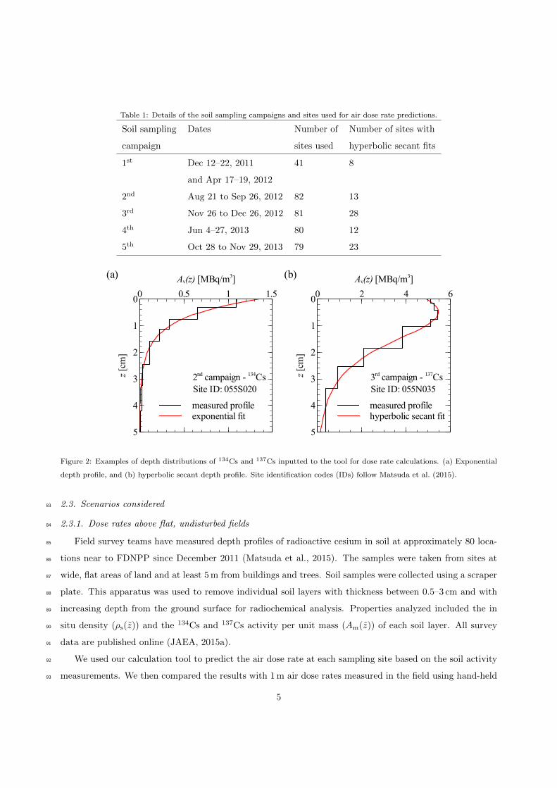
Table 1: Details of the soil sampling campaigns and sites used for air dose rate predictions.

Soil sampling

campaign

Dates Number of

sites used

Number of sites with

hyperbolic secant fits

1st Dec 12–22, 2011

and Apr 17–19, 2012

41 8

2nd Aug 21 to Sep 26, 2012 82 13

3rd Nov 26 to Dec 26, 2012 81 28

4th Jun 4–27, 2013 80 12

5th Oct 28 to Nov 29, 2013 79 23

(a)

measured profileexponential fit

Site ID: 055S0202nd campaign - 134Csz [

cm]

0

1

2

3

4

5

Av(z) [MBq/m3]0 0.5 1 1.5

(b)

measured profilehyperbolic secant fit

Site ID: 055N0353rd campaign - 137Csz [

cm]

0

1

2

3

4

5

Av(z) [MBq/m3]0 2 4 6

Figure 2: Examples of depth distributions of 134Cs and 137Cs inputted to the tool for dose rate calculations. (a) Exponential

depth profile, and (b) hyperbolic secant depth profile. Site identification codes (IDs) follow Matsuda et al. (2015).

2.3. Scenarios considered83

2.3.1. Dose rates above flat, undisturbed fields84

Field survey teams have measured depth profiles of radioactive cesium in soil at approximately 80 loca-85

tions near to FDNPP since December 2011 (Matsuda et al., 2015). The samples were taken from sites at86

wide, flat areas of land and at least 5 m from buildings and trees. Soil samples were collected using a scraper87

plate. This apparatus was used to remove individual soil layers with thickness between 0.5–3 cm and with88

increasing depth from the ground surface for radiochemical analysis. Properties analyzed included the in89

situ density (ρs(z)) and the 134Cs and 137Cs activity per unit mass (Am(z)) of each soil layer. All survey90

data are published online (JAEA, 2015a).91

We used our calculation tool to predict the air dose rate at each sampling site based on the soil activity92

measurements. We then compared the results with 1 m air dose rates measured in the field using hand-held93

5

survey meters. Data over five soil sampling campaigns were considered in the analysis. The dates of the94

campaigns are listed in Table 1. The measured activity depth profiles (Am(z)) were scaled into activity95

concentration profiles applicable for the tool (Av(z)) using the procedure described in section 2.2. Examples96

of the processed depth profiles for two sites are shown in Fig. 2 (black lines).97

As a scraper plate sample was taken at only one point on the ground per location visited in each soil98

sampling campaign, it was assumed that the measured soil activity depth distribution applied homogeneously99

across the whole region simulated by the tool. Explicitly, the activity concentrations for each soil layer100

inputted to the tool were identical across all cells on the simulation mesh.101

We also considered a second method for evaluating air dose rates from the soil activity samples, based102

on modelling empirical fits to the activity depth profiles. Matsuda et al. (2015) characterized the activity103

depth profiles as a function of mass depth (Am(ζ)) by fitting exponential and hyperbolic secant functions.104

The exponential depth distribution is105

Am(ζ) = Am,0 exp (−ζ/β) , (6)

where Am,0 (Bq/kg) is the activity per unit soil mass at the ground surface and β (g/cm2) is the relaxation106

mass depth that characterizes the degree of fallout penetration into the soil. Figure 2(a) shows a fit of the107

exponential function to soil layer activity measurements at one site. The total inventory of contamination108

per unit area of land for this distribution is:109

Ainv = 10βAm,0 . (7)

The factor of 10 ensures Ainv has units of Bq/m2. The exponential distribution is a satisfactory model for110

the soil activity depth profile for the first few years after fallout deposition (ICRU, 1994).111

Matsuda et al. (2015) observed that some of the measured depth profiles display a maximum in the112

radiocesium concentration below the ground surface. They proposed fitting a hyperbolic secant function to113

these depth profiles, as this function can reproduce a peak in activity concentration below the surface. The114

hyperbolic secant function is115

Am(ζ) = Am,0 cosh (ζ0/β)sech(−(ζ − ζ0)/β) . (8)

Again Am,0 (Bq/kg) is the activity per unit soil mass at the ground surface, and β (g/cm2) is a parameter116

characterizing the length scale of the distribution. The peak in activity occurs at the mass depth ζ0 (g/cm2)117

below the surface. The hyperbolic secant function converges to an exponential distribution at large mass118

depths. Figure 2(b) shows a fit of the hyperbolic secant function to a measured depth distribution. The119

total radionuclide inventory per unit area for the hyperbolic secant distribution is120

Ainv = 20βAm,0 cosh (ζ0/β)[(π/4) + tan−1 (tanh (ζ0/(2β)))] . (9)

6

We followed Matsuda et al. (2015) and fitted the exponential and hyperbolic secant distributions to measured121

depth profiles. The hyperbolic secant function was used for profiles displaying a peak in activity below the122

surface, and the exponential function otherwise. Table 1 lists the number of sites in this analysis and the123

number of fits with the hyperbolic secant function. Examples of the fitted distributions are shown for two124

sites in Fig. 2 (red lines)125

We discounted from the analysis any depth profiles showing signs of soil mixing or disturbance (Matsuda126

et al., 2015). Soil disturbance included land cultivation and decontamination work. We also discounted sites127

where the air dose rate was not measured with a survey meter at the time of collecting the soil samples.128

Modelling both the measured and the empirical fits for the soil depth profiles yielded two predictions129

for the air dose rate at each site. The air dose rate was calculated as the sum of contributions from 134Cs130

and 137Cs, and an additional 0.05 µSv/h contribution representing the background dose rate from natural131

radionuclides (Mikami et al., 2015b).132

2.3.2. Evolution of air dose rates133

In addition to the soil sampling campaigns, JAEA and partners have been measuring air dose rates with134

hand-held survey meters at thousands of locations across Fukushima Prefecture, including locations with135

flat, undisturbed fields (Saito et al., 2015; Mikami et al., 2015b). The monitoring results show that dose rates136

at these locations decreased faster than expected by just the physical decay of 134Cs and 137Cs (Saito and137

Onda, 2015). Mikami et al. (2015a) demonstrated that, for the period between March 2012 and December138

2012, relatively little migration of the 137Cs inventory away from these fields occurred. Mikami et al.139

(2015b) explained the decrease in dose rates, beyond what could be expected by radioactive decay alone, by140

the downward migration of radioactive cesium into the soil.141

The relaxation mass depth, β, characterizes the penetration of fallout into soil for the exponential142

distribution (Eq. 6). Conversion coefficients published for various values of β can be used to evaluate the143

1 m ambient dose equivalent rate given the radionuclide inventory per unit area of soil (Saito and Petoussi-144

Henss, 2014). In contrast, two parameters characterize the penetration of the radionuclides within soil for145

the hyperbolic secant distribution - a relaxation mass depth β and a mass depth ζ0 for the peak in activity146

concentration below the surface (Eq. 8).147

To allow direct comparison between exponential and hyperbolic secant depth profiles, Matsuda et al.148

(2015) proposed an effective relaxation mass depth parameter, βKeff (g/cm2), for the hyperbolic secant dis-149

tribution. The effective relaxation mass depth is defined as the value β of an exponential depth distribution150

yielding the same air kerma rate at 1 m as the hyperbolic secant distribution (K - µGy/h), given an identical151

inventory of fallout radionuclides in both distributions (i.e. Ainv is equal for both distributions).152

In this study we used our calculation tool to calculate effective relaxation mass depths for the hyperbolic153

secant fits over the five soil sampling campaigns. The effective relaxation mass depths were calculated154

7

Table 2: Data for βHE∗(10)eff over the five soil sampling campaigns.

Soil sampling

campaign

Number of

sites used

Number of sites with

hyperbolic secant fits

Mean βHE∗(10)eff

(g/cm2)

Median βHE∗(10)eff

(g/cm2)

Min βHE∗(10)eff

(g/cm2)

Max βHE∗(10)eff

(g/cm2)

1st 83 12 1.13 0.93 0.24 5.95

2nd 82 13 1.41 1.00 0.11 8.72

3rd 81 28 1.56 1.23 0.43 10.36

4th 80 12 1.64 1.36 0.29 7.73

5th 79 23 2.17 1.85 0.38 6.41

by matching HE ∗ (10) from each hyperbolic secant distribution to an exponential distribution of equal155

inventory, i.e. βHE∗(10)eff (g/cm2). Note that the definition of effective relaxation mass depth means that156

βHE∗(10)eff for an exponential distribution is equal to the relaxation mass depth (β) of the distribution.157

We calculated arithmetic mean, median, minimum and maximum βHE∗(10)eff values for each of the five158

soil sampling campaigns (Table 2). More sites from the first soil sampling campaign could be used in this159

analysis than for the dose rate predictions (c.f. Table 2 with Table 1), as it was not necessary to have a field160

survey measurement of the air dose rate in order to calculate βHE∗(10)eff .161

We considered the decrement of the components of the air dose rate attributable to radioactive cesium162

fallout, i.e. HE ∗ (10) measurements minus a 0.05 µSv/h contribution from natural background radiation,163

over the first four air dose rate surveys (JAEA, 2015a). The dates of the air dose rate surveys and the mean164

air dose rates at flat, undisturbed fields are listed in Table 3.165

We modelled the decrement in dose rates due to radioactive decay and cesium migration deeper within166

soil. First, we matched the mean βHE∗(10)eff values from the soil sampling campaigns to the periods of the167

air dose rate surveys (Table 3). We then modelled exponential distributions with β parameters equal to the168

mean βHE∗(10)eff values with the tool. The inventories supplied were decay corrected to dates at the middle169

of each air dose rate survey period. The decay corrections assumed an activity ratio of released 134Cs and170

137Cs from FDNPP of 1.00 on March 11, 2011 (UNSCEAR, 2014). The results show little sensitivity to171

plausible alternatives (in the range 0.90–1.08) for this initial activity ratio. The calculated dose rates were172

then normalized to June 21, 2011, the date at the middle of the first air dose rate survey (Table 3), for173

comparison with the measured dose rates. As no scraper plate soil samples were available for the period174

of the first air dose rate survey (June 4 to July 8, 2011), a βHE∗(10)eff value of 1.00 g/cm2 was assumed as175

applicable for this period (Mikami et al., 2015b). The sensitivity of the results upon this assumption is176

checked in the results section.177

8

Table 3: Details of the air dose rate surveys and results for the models of dose rate reductions. aAssumed value. See text for

details.

Air dose rate survey Soil sampling Mean βHE∗(10)eff Measurements Models

Campaign Dates campaign (g/cm2) H∗(10) - 0.05

(µSv/h)

Relative

change

Decay

only

Decay &

migration

1st campaign Jun 4 to

Jul 8, 2011

- 1.00a 1.25 1.0 1.0 1.0

2nd campaign Dec 13, 2011 to

May 29, 2012

1st 1.13 1.01 0.81 0.84 0.82

1st part of 3rd

campaign

Aug 14 to

Sep 7, 2012

2nd 1.41 0.84 0.67 0.76 0.70

2nd part of 3rd

campaign

Nov 5 to

Dec 7, 2012

3rd 1.56 0.78 0.62 0.72 0.65

1st part of 4th

campaign

Jun 3 to

Jul 4, 2013

4th 1.64 0.64 0.51 0.64 0.57

2nd part of 4th

campaign

Oct 28 to

Dec 2, 2013

5th 2.27 0.55 0.44 0.59 0.48

0 100 200 [m]

N

1 Decontaminated area

0 500 [m]

Modified from 1:25,000 Topographic Maps ©Geospatial Information Authority of Japan

Paddy field

Truck farm

BuildingsWasteland

Coniferous forest

N

Fukushima Dai-ichi NPP

Okuma town

Points of measurement

Grid for simulation

No.4

No.14

No.15

No.18No.16

No.13

No.10No.12

No.11

No.1No.2 No.3

No.6

No.9No.7

No.8No.5

No.17

Figure 3: The decontamination boundary and soil sampling locations at Ottozawa.

9

137Cs measured137Cs exponential fit134Cs measured134Cs exponential fit

(a)

β = 3.60 g/cm2Ottozawa - Location 5

z [cm

]0

2

4

6

8

Av(z) [MBq/m3]0 20 40 60 80

137Cs measured137Cs exponential fit134Cs measured134Cs exponential fit

(b)

β = 1.83 g/cm2Ottozawa - Location 14

z [cm

]

0

2

4

6

8

Av(z) [MBq/m3]0 5 10 15 20

Figure 4: Measured soil activity depth distributions and exponential fits for the Ottozawa area. (a) Location 5, and (b)

location 14.

2.3.3. Spatial variability in soil activity levels178

The calculations with the tool in sections 2.3.1 and 2.3.2 assumed spatially uniform radiocesium distri-179

butions, as only one soil sample was available at each location. We considered the effect of spatial variability180

in the radiocesium distribution on evaluating dose rates by studying the Ottozawa area. The area lies within181

2 km of FDNPP and soil samples were taken at multiple locations across the paddy fields and scrubland in182

the area. Figure 3 shows a map of the area and the soil sampling locations.183

This area was remediated between November 2011 and May 2012 as part of a decontamination pilot184

project coordinated by JAEA and is now subject to long-term environmental monitoring (JAEA, 2015b).185

Remediation consisted of removing the top 5 cm of topsoil from paddy fields and areas around residential186

buildings, and cleaning road and building surfaces. The air dose rates ranged from 22–263µSv/h before187

decontamination, and dropped to between 4–110µSv/h afterwards. Decontamination of this area was studied188

numerically by Hashimoto et al. (2014).189

The soil samples and air dose rates were taken on July 24, 2014 at 18 locations across the area. Soil190

samples were collected by inserting a cylindrical plastic cup (U-8 type, 58 mm internal height, 50 mm internal191

diameter) into the topsoil and collecting the soil contents into plastic bags (Onda et al., 2015). One sample192

was taken at locations 1–16, while five samples were collected for locations 17 and 18. Locations 17 and 18193

lie outside the decontaminated area.194

The 134Cs and 137Cs depth distributions at locations 5 and 14 were determined by using a scraper plate195

to remove 1 cm thick soil layers down to a maximum depth of 10 cm. The activity per unit soil mass in each196

layer was measured using a high resolution gamma spectrometer. Unfortunately due to oversight we did197

not measure the in situ densities at the time of collecting the soil samples. Therefore we had to make an198

10

0 100 200 [m]

N

No.4

No.14

No.15

No.18No.16

No.13

No.10No.12

No.11

No.3

No.6

No.9No.7

No.8No.5

No.17

137Cs inventory [Bq/m2]

1E+5 1E+6 1E+7 1E+8

No.2No.1

Figure 5: 137Cs inventories assigned to cells across the Ottozawa area for simulation of air dose rates at locations 1–18.

assumption for the layer densities. We chose densities equal to the mean densities of the soil layers collected199

over the five scraper plate sampling campaigns described in section 2.3.1. The measured activity depth200

profiles at Ottozawa were exponential to a reasonable approximation (Fig. 4).201

Scraper plate analyses of the activity depth distributions were not performed at the other locations202

(locations 1–18, excluding 5 and 14). An exponential depth distribution was assigned to these locations203

based on the β value applicable at the nearest of locations 5 and 14 to the site. Locations 1–9 were thus204

assigned an exponential depth distribution with β = 3.60 g/cm2, and locations 10–18 an exponential depth205

distribution with β = 1.83 g/cm2. The total inventory per unit area, Ainv, was inferred by correcting206

the cylindrical cup activity measurement for radioactivity at depths greater than 58 mm as given by the207

exponential distribution. The inventory for locations 5, 14, 17 and 18, where multiple soil samples were208

taken, was taken to be the mean over the various samples.209

Two strategies were used to predict the air dose rate at locations 1–18. The first strategy assumed that210

the radiocesium distribution was spatially homogeneous. The inventory and depth distribution for that211

location was applied uniformly across the simulation region.212

The second strategy was to model the spatial heterogeneity in soil activity levels, as revealed by the213

11

Am(z) [kBq/kg]0 0.5 1 5 10 15 20

~

~

(a)

134Cs

z [cm

]

0

10

20

30

Am(z) [kBq/kg]0 0.5 1 5 10 15 20

~

~

Before remediationTopsoil removalReverse tillageLayer interchange

(b)

137Csz [

cm]

0

10

20

30

Figure 6: Activity depth distributions of 134Cs and 137Cs for three farmland soil remediation methods, shown for the in situ

depth coordinate z. Note break in horizontal axes at 1 kBq/kg to show full distribution of activity with depth.

soil samples at the other locations. A 12.5 by 12.5 m mesh was overlaid onto a map of the area (Fig. 3).214

Cells containing a soil sampling location were assigned the inventory and relaxation mass depth for that215

sample. We adopted a simple interpolation method to assign inventories and relaxation mass depths to216

the other cells on the mesh. The inventories and β values were set equal to the values applicable at the217

nearest cell hosting a sampling location. Cells equidistant from more than one sampling location were218

assigned inventories randomly from one of the equidistant locations. Because of a large disparity between219

soil activity levels inside and outside the bounds of the remediated area, locations outside the remediated220

area were assigned the inventory of the closest of either location 17 or 18. It would also be possible to221

employ other interpolation techniques to assign inventories to cells without soil samples, for example based222

on inverse distance weighting techniques or Kriging (IAEA, 2003).223

The assigned inventories for all cells across the area are depicted in Fig. 5. The mesh size simulated in224

the tool was 149 by 149 cells for both dose rate prediction methods.225

2.3.4. Evaluation of farmland soil remediation methods226

To evaluate different methods for remediating farmland soils, we used the tool to calculate air dose rates227

after remediation by topsoil removal, reverse tillage, or topsoil-subsoil layer interchange. Figure 6 shows a228

typical exponential depth distribution for 134Cs and 137Cs within undisturbed farmland soil in Fukushima229

Prefecture (solid black lines). The 134Cs to 137Cs activity ratio is applicable on December 01, 2011. This date230

falls within a pilot project on decontamination techniques, and allows comparison of dose rate predictions231

from the tool against environmental measurements from the decontamination project (JAEA, 2015b).232

The relaxation mass depth of the exponential profile in Fig. 6 is β = 1.13 g/cm2. This follows the result233

from the first soil depth distribution sampling campaign (Table 2). The air dose rate under these 134Cs and234

12

137Cs inventories and depth profiles is 1.25 µSv/h before remediation, including a 0.05 µSv/h contribution235

from natural background radiation.236

The different remediation methods alter the activity depth distributions of the farmland soil. Figure237

6 shows idealized activity depth distributions after topsoil removal, reverse tillage, or topsoil-subsoil layer238

interchange. We used the tool to evaluate the air dose rate after completion of each of these remediation239

options.240

Topsoil removal involves mechanically stripping the top 5 cm of the soil, and disposing the excavated soil241

as radioactive waste. The activity profile for the remaining soil is, to a first approximation, the exponential242

distribution for depths greater than 5 cm prior to decontamination (dotted red lines in Fig. 6).243

Reverse tillage employs a tractor pulled plough to invert the topsoil. The ploughing creates small ridges244

and furrows on the land surface, which flatten off as the soil weathers and relaxes. We approximated the245

soil as being homogeneously mixed after this process. Ploughing down to a depth of 25 cm thus results in a246

constant radioactivity profile initially with depth, followed by the exponential distribution at depths below247

25 cm (dashed blue lines in Fig. 6).248

In Topsoil-subsoil layer interchange a layer of topsoil is switched with a layer of subsoil. Typically a249

topsoil layer down to 15 cm is excavated with a digger and this soil is placed aside on a plastic sheet. The250

next 15 cm of subsoil is then excavated and stored temporarily on adjacent ground. The pit that has been251

created is refilled by first adding a 15 cm layer of the original topsoil, and then levelling to the ground surface252

with the excavated subsoil layer. This strategy can be approximated as creating two homogenized layers of253

activity concentration below the ground surface. The top layer, down to 15 cm depth, contains the activity254

originally between the depths of 15 cm and 30 cm. The subsequent 15 cm thick layer below contains the255

activity that was originally in the top 15 cm of soil (green dash-dot lines in Fig. 6).256

To model these remediation scenarios, we considered remediation of a 37.5 by 37.5 m (1.4 km2) area257

of land, equivalent to a 3 by 3 square of cells on the simulation mesh (Fig. 7). The simulation models258

consisted of remediated depth distributions within these cells, while the depth distributions outside the area259

remained unchanged. Reductions in the dose rates were calculated for the center and near to the corners260

of the remediated square of land. All dose rate evaluations included a 0.05 µSv/h contribution from natural261

background radiation.262

3. Results and discussion263

3.1. Dose rates above flat, undisturbed fields264

The predictions for air dose rates above flat, undisturbed fields made using the measured activity depth265

profiles compare well with the dose rates measured at the sampling sites, as shown by Fig. 8(a). The266

correlation holds over the range of dose rates covered by the dataset (0.09–5.3 µSv/h). The predicted dose267

13

37.5

m

37.5 m

Figure 7: Setup of farmland soil remediation simulations: light blue area within orange dashed line is remediated land. Land in

the dark blue area outside is not remediated. Dose rates before and after remediation were calculated for the locations marked

by black spots.

(a)

R2 = 0.825

Exact depth profiles

Sim

ulat

ed H*(

10) [

μSv/

h]

0.1

1

10

Measured H*(10) [μSv/h]0.1 1 10

(b)

1st campaign2nd campaign3rd campaign4th campaign5th campaign

Exact depth profiles

Resid

ual [

μSv/

h]

−3

−2

−1

0

1

2

3

Measured H*(10) [μSv/h]0.1 1 10

Figure 8: Correlation between measured air dose rates from the soil sampling campaigns and simulation predictions using

measured soil depth profiles as inputs. (a) Measurement-prediction correlation. The dotted line indicates y = x. (b) Scatter

plot of residual errors in the predictions. The dotted line is y = 0.

14

(a)

R2 = 0.785

Empirical fits

Sim

ulat

ed H*(

10) [

μSv/

h]

0.1

1

10

Measured H*(10) [μSv/h]0.1 1 10

(b)

1st campaign2nd campaign3rd campaign4th campaign5th campaign

Empirical fits

Resid

ual [

μSv/

h]−3

−2

−1

0

1

2

3

Measured H*(10) [μSv/h]0.1 1 10

Figure 9: As per Fig. 8, except showing dose rate predictions made the exponential and hyperbolic secant fits to the measured

soil activity depth distributions.

rates are always within a factor of three of the true dose rate, with one exception. At one site a dose rate268

of 0.87 µSv/h was observed, but the tool predicted 0.075 µSv/h.269

The residual differences between the predictions and the measured dose rates are shown in Fig. 8(b). A270

positive residual indicates an over-estimation by the tool, and a negative residual, an under-estimate. There271

is no tendency for the tool to either over-estimate or under-predict dose rates across the range of dose rates272

measured in the surveys.273

Tyler et al. (1996) noted previously that individual soil samples can be poor representations of the mean274

soil activity across a wide area. The mean free path in air of the primary gamma rays emitted by 134/137Cs275

decay is around 100 m. Satoh et al. (2014) showed that radioactivity within 500 m contributes significantly276

to an air dose rate. Thus, the total volume of soil contributing to the dose rate, down to a depth of 8 cm,277

is 62 800 m3. As the volume of soil collected down to the same depth with a 15 cm by 30 cm scraper plate278

is 0.0036 m3, the sample represents only 6 · 10−8 parts of the total soil volume contributing to the air dose279

rate.280

Highly variable 134Cs and 137Cs activity concentrations are often found between different soil samples281

taken at the same location. Saito et al. (2015) confirmed this was the case for soil samples taken in Fukushima282

Prefecture. The variations are caused by heterogeneity in the fallout deposition, and by scrubbing and283

concentration of fallout nuclides by local earth surface processes. Therefore, a large sampling uncertainty284

for the inventory of the total soil volume contributing to the air dose rate should be expected if only a single285

soil sample is available. We ascribe the sampling uncertainty from the scraper plate measurement as the286

main source of error in the predictions for the air dose rate shown in Fig. 8(a).287

We next considered the quality of the dose rate predictions obtained by modelling the empirical fits to288

15

the measured depth profiles (Fig. 9(a)). The coefficient of determination obtained in this case is slightly289

lower than the models employing the measured depth profiles directly (R2 = 0.785 versus 0.825). The290

slight difference in R2 values is caused by the predictions for the high dose rate locations being slightly less291

accurate from the models employing the empirical fitting functions. The residual errors for the predictions292

at these high dose rate locations dominate the squared residuals sum in the calculation of R2, and hence293

the resulting R2 value.294

The residuals for the predictions obtained by modelling the empirical fits are shown in Fig. 9(b). Exclud-295

ing the high dose rate locations, the amount of scatter in the residuals is comparable to Fig. 9(a). Another296

way to quantify the accuracy of the predictions is to consider the mean absolute percentage error. This297

statistic is less susceptible to being skewed by the squared residuals for the predictions at the high dose298

rate locations than R2. The mean absolute percentage error of the predictions made using the exact depth299

profiles is 29 %. This compares with a mean absolute percentage error of 30 % for the predictions obtained300

by modelling the fitted activity depth profile functions.301

The results thus indicate that no significant error is introduced by modelling the empirical fits to the302

activity depth profiles instead of the measured step-wise profiles. This conclusion necessarily depends on the303

details of the soil sampling procedure. Matsuda et al. (2015) measured the activity within 0.5 cm layers of304

topsoil, followed by 1 and 3 cm thick layers at deeper depths. If coarser soil layer thicknesses are employed,305

modelling the empirical fits may yield more accurate predictions than modelling the measured depth profiles,306

as it is plausible for the empirical fits to offer a better representation of the true activity profile in the soil.307

3.2. Evolution of air dose rates308

The distributions of βHE∗(10)eff values obtained from the exponential and hyperbolic secant fits to the309

depth profiles are shown in Fig. 10(a) for the five soil sampling campaigns. Both the mean and median310

values of βHE∗(10)eff increase over time (Table 2), indicating that the radiocesium is migrating deeper into the311

soil.312

The component of the mean air dose rate attributable to radiocesium at the flat, undisturbed fields is313

plotted for the air survey campaigns with solid diamonds in Fig. 10(b). The data are plotted relative to314

June 2011, the date of the first air dose rate survey (Table 3).315

The solid line in Fig. 10(b) represents the decrement in dose rates that would be expected on the basis of316

radioactive decay of 134Cs and 137Cs, and without migration of the radiocesium at the sites. The measured317

dose rates decrease faster than expected by just radioactive decay.318

Mikami et al. (2015b) explained the additional reduction in dose rates between June 2011 and December319

2012 by migration of the cesium fallout deeper into the soil pack. This trend continued through 2013, as320

shown by the results of our decay and migration calculations (open circles, Fig. 10(b)). The decay and321

16

(a)

β effH*(

10) [g

/cm

2 ]

0.1

1

10

Month/Year12/11 06/12 12/12 06/13 12/13

(b)

MeasurementsDecay only modelDecay & migration

H* (1

0) -

0.05

[nor

mali

zed

to 0

6/20

11]

0.4

0.6

0.8

1

Month/Year

06/11 12/11 06/12 12/12 06/13 12/13

Figure 10: (a) Box and whisker plot showing distribution of βHE∗(10)eff values over the five soil sampling campaigns. The

whiskers show the maxima and minima of the distributions. The boxes show the range in between the 25th and 75th percentiles

of distributions. The mean values are indicated by asterisks. The full distributions are plotted with symbols, offset to the left

of each box and whiskers. (b) Measurements and modelling results for the reduction in air dose rate component attributable

to radioactive cesium at locations of flat, undisturbed fields. The measurements (solid diamonds) show the mean air dose rate

attributable to radiocesium from the air survey campaigns, normalized to the value at the first air dose rate survey (Table 3).

The vertical bars on the data for the decay and migration model (circles) indicate results when varying βHE∗(10)eff between

0.5–2.0 g/cm2 at the time of the first air dose rate survey (June 2011).

17

migration model results are reasonably consistent with the measurements, although they tend to under-322

estimate the reduction in dose rates by up to 10 %.323

A source of uncertainty in the decay and migration model is the choice for mean βHE∗(10)eff for the first324

air dose rate survey campaign (June 4 to July 8, 2011 - Table 3). The soil sampling campaigns by Matsuda325

et al. (2015) commenced in December 2011, so cannot provide measurements to derive a mean βHE∗(10)eff326

value applicable to this period. The circles in Fig. 10(b) represent the assumption that βHE∗(10)eff = 1.0 g/cm2

327

in June 2011. ICRU (1994) cites β values for atmospheric radionuclide fallout in the range 0.1–4 g/cm2 for328

up to one year after fallout deposition. These results are based on measurements for cesium radioisotopes329

from Chernobyl fallout in Europe and Western Russia.330

Takahashi et al. (2015) measured depth distributions at two grassland sites and three abandoned agricul-331

tural fields in Fukushima Prefecture between June 21–28, 2011. They found that the exponential distribution332

was a good fit for the measured depth profiles, with β values in the range 0.60–3.08 g/cm2. However, they333

noted that the site giving the highest relaxation mass depth (3.08 g/cm2) was pasture land where the soil334

had been disturbed by cattle grazing. Excluding this site from their dataset yields a mean β value from four335

sites of 1.20 g/cm2.336

To determine the sensitivity of our decay and migration model on the choice for the mean βHE∗(10)eff337

value for the first air dose rate survey, we considered the effect of varying this parameter in the range 0.50–338

1.20 g/cm2. This is a range of values that we consider credible for the period between June 4 and July 8,339

2011, based on the previous literature cited and the mean βHE∗(10)eff value of 1.13 g/cm2 derived from the340

first soil sampling campaign in December 2011 (Table 2). The effect of varying the initial value of βHE∗(10)eff341

in this range is shown by vertical bars around circle markers in Fig. 10(b). The ranges indicated by these342

bars include the measurements, but do not permit the decay only explanation for the reduction in dose343

rates. The sensitivity analysis is thus consistent with the conclusion that migration of cesium deeper into344

the ground was the main cause behind the additional decrement in dose rates.345

There are two other factors that could plausibly explain the underestimation of the true dose rate346

reduction by the model for decay and migration deeper into soil (Fig. 10(b)). Although Mikami et al. (2015a)347

suggested that little migration of the radiocesium inventory in the horizontal direction had occurred, within348

uncertainties their data are consistent with a possible small amount of horizontal migration (on the order349

of 5–10 % of the inventory).350

Another factor is as follows. Although the sites featuring in the air dose rate surveys were chosen to be351

flat, open spaces (Mikami et al., 2015b), certain sites may include urban areas or areas with roads and paved352

surfaces at the periphery. The wide field of view of environmental radioactivity means that radiocesium353

within these areas contributes to the air dose rate. As the radiocesium within these areas has a shorter354

ecological half-life than areas of glassland or agricultural areas (Kinase et al., 2014), i.e. the radiocesium is355

more easily washed away, this could contribute to the underestimation of the dose rate reduction by the356

18

(a)

R2 = 0.590

Homogeneous inventorySi

mul

ated

H*(

10) [

μSv/

h]

1

10

100

Measured H*(10) [μSv/h]1 10 100

(b)

R2 = 0.753

Heterogeneous inventory

Sim

ulat

ed H*(

10) [

μSv/

h]

1

10

100

Measured H*(10) [μSv/h]1 10 100

Figure 11: Correlation between measured air dose rates and predictions from soil activity levels at Ottozawa. (a) Assumed a

spatially homogeneous 134Cs and 137Cs inventory. (b) Spatially varying inventory informed by all the soil sampling locations.

Triangles indicate locations 5 and 14, where scraper plate samples yielded the depth distribution.

models in Fig. 10(b).357

3.3. Effect of spatial variability in soil activity levels358

The Ottozawa area was used to study the effect of spatial variations in the radiocesium distribution on359

air dose rates. The range of dose rates measured at Ottozawa in July 2014 varied between 3.5–41.4 µSv/h360

(Table 4). This is a higher range of values than measured in the five soil sampling campaigns (section 3.1),361

as Ottozawa lies closer to FDNPP than the sites in the five soil sampling campaigns and is more highly362

contaminated with fallout from the accident.363

Fig. 11 shows two sets of predictions for the air dose rates from soil activity measurements, plotted364

against the dose rates measured in the field. The predictions shown in Fig. 11(a) did not account for the365

spatial variations in soil activity levels. Figure 11(b) shows predictions from the models incorporating the366

measured spatial variations in the cesium inventory.367

It is clear that modelling the spatial variations in the contamination distribution yields better predictions368

for the air dose rate. Therefore modelling the spatial variation is the better strategy if multiple soil samples369

across an area are available to include in the dose rate analysis.370

The coefficient of determination is higher for the predictions modelling the spatial distribution (R2 =371

0.753) than for the predictions assuming a homogeneous radiocesium distribution (R2 = 0.590). The origin372

of the difference in the R2 values is traceable to the model accounting for the spatial distribution yielding a373

better prediction for the highest dose rate site, location 17, with a measured dose rate of 41.4 µSv/h, than374

the model assuming a homogeneous cesium distribution.375

19

Table 4: Results of soil sampling and air dose rate predictions for Ottozawa area on July 24, 2014. Bold indicates soil samples

taken with scraper plate apparatus. Other samples collected with U-8 cup. Italic indicates values of β inferred from depth

distributions at locations 5 or 14.

Location Inventory

(MBq/m2)

β

(g/cm2)

Measured H∗(10)

(µSv/h)

Prediction based on assumption

for Cs distribution (µSv/h)

134Cs 137Cs Homogeneous Heterogeneous

1 0.643 1.89 3.60 14.6 5.3 9.5

2 0.154 0.453 3.60 7.4 1.3 5.7

3 0.472 1.43 3.60 8.2 3.9 9.2

4 0.294 0.868 3.60 13.0 2.4 5.7

5 0.567

0.483

1.67

1.47

3.60 6.9 4.3 8.3

6 2.24 6.61 3.60 12.1 18.2 19.9

7 0.141 0.419 3.60 6.6 1.2 5.6

8 0.189 0.566 3.60 7.1 1.6 7.8

9 1.82 5.52 3.60 8.1 15.0 15.2

10 0.265 0.811 1.83 7.1 2.7 7.7

11 0.0342 0.122 1.83 4.1 0.4 3.0

12 0.258 0.758 1.83 3.5 2.6 5.6

13 0.305 0.888 1.83 5.4 3.1 9.3

14 0.0714

0.0506

0.210

0.145

1.83 3.6 0.7 4.6

15 0.0391 0.114 1.83 3.5 0.4 6.6

16 0.665 1.95 1.83 6.9 6.7 12.6

17 8.78

7.88

12.4

9.95

9.68

26.1

23.7

37.4

29.3

29.0

1.83 41.4 98.0 89.7

18 9.37

2.17

3.95

4.42

2.41

27.8

6.34

11.8

13.3

7.22

1.83 27.6 44.9 38.8

20

(a)Location 5 - cv = 0.52Location 14 - cv = 0.39

137 Cs

inve

ntor

y [M

Bq/m

2 ]

0

0.5

1

1.5

2

Soil SampleSP C1 C2* C3* C4* C5* C6* SP C1 C2* C3* C4* C5* C6*

(b)Location 17 - cv = 0.16Location 18 - cv = 0.58

137 Cs

inve

ntor

y [M

Bq/m

2 ]

0

10

20

30

40

Soil SampleC1 C2 C3 C4 C5 C1 C2 C3 C4 C5

Figure 12: Variation in 137Cs inventory between soil samples at Ottozawa locations 5, 14, 17 and 18. SP denotes a scraper plate

sample, and C1, C2, etc. denote the U-8 cup samples. Asterisks denote soil samples taken on October 10, 2014 and inventory

decay corrected to July 24, 2014. cv denotes coefficient of variation between the soil sample inventories at each location. cv is

the ratio of the sample standard deviation to the mean.

The mean absolute percentage error for the predictions taking into account the spatial heterogeneity of376

the activity is 47 %. This result is higher than the ≈30 % mean absolute percentage error for the predictions377

for dose rates above flat, undisturbed fields (section 3.1). This difference is also observable by comparing378

the quality of the correlation in Figs. 8(a) and 9(a) with Fig. 11(b).379

There are a number of distinctions between the modelling at Ottozawa and the flat, undisturbed fields380

that contribute to a higher uncertainty for the predictions at Ottozawa. There is a higher degree of mea-381

surement uncertainty for many of the soil samples at Ottozawa than for the sites visited in the five soil382

sampling campaigns, as the U-8 cup samples collect smaller volumes of soil than the scraper plate. This383

can be shown by examining the inventories from the multiple soil samples taken at locations 5, 14, 17 and384

18 (Fig. 12). There is large variation between the inventories between the samples at each location. The385

highest variation is seen for location 18, where the largest inventory is four times greater than the smallest386

inventory.387

The mean coefficient of variation for the four Ottozawa locations is cv = 0.41. This is larger than the388

mean cv = 0.36 observed by Saito et al. (2015) for locations within a 100 km radius of FDNPP, which are389

similar to the sites visited in the soil sampling campaigns. Mishra et al. (2015) independently reported a390

coefficient of variation of 0.27 between four samples at another site similar to those visited in the Matsuda391

et al. (2015) soil sampling campaigns.392

Another factor contributing to the uncertainty for the predictions at Ottozawa include the fact that393

scraper plate samples were only taken at locations 5 and 14. The depth distribution at other locations394

had to be inferred from these two measurements. It is notable that some of the best dose rate predictions395

obtained for Ottozawa were at locations 5 and 14 (triangles - Fig. 11(b)).396

21

Table 5: The percentage reduction in the air dose rate after remediation of farmland soils by three different methods. The

simulation input data (depth profiles, activity levels, etc.) were applicable on December 01, 2011. Full remediation means that

all 149 by 149 cells on the simulation mesh were modelled as remediated land.

Remediation Observed Simulation results

method results

(JAEA, 2015b)

Centre of 37.5 by 37.5 m

remediated area

Corner of 37.5 by 37.5 m

remediated area

Full

remediation

Topsoil removal 40–70 % 73 % 65 % 96 %

Reverse tillage 30–60 % 54 % 46 % 71 %

Topsoil-subsoil

layer interchange

≈65 % 68 % 60 % 90 %

3.4. Evaluation of farmland soil remediation methods397

We used the tool to evaluate the effectiveness of three methods for remediating farmland soils for de-398

creasing air dose rates (Table 5). We calculated the reduction in air dose rate at the center and the corner399

of a 37.5 by 37.5 m square area of remediated land, and compared with field results from a decontamination400

pilot project in Fukushima Prefecture (JAEA, 2015b). Also shown in Table 5 are theoretical limits for the401

reduction in dose rates, calculated assuming remediation of all the land surface.402

The performance of the topsoil removal and layer interchange methods of remediation are similar. Both403

methods yield ≈65 % reduction in air dose rates for the square area of remediated land. These methods are404

more effective than reverse tillage, where the calculations indicated a ≈50 % reduction in the air dose rate.405

Experience from the decontamination pilot project (JAEA, 2015b) suggests a range of dose rate reduc-406

tions for topsoil removal and reverse tillage. A number of factors affect the percentage reduction in dose407

rates after land remediation, including the size of the area remediated, the homogeneity of the remediation408

actions, and the magnitude of the dose rate before remediation relative to the natural background dose409

rate. The remediation parameters, e.g. the thickness of topsoil removed, or the depth of ploughing when410

performing reverse tillage, may also have varied slightly. However, the general correspondence in Table 5411

between the predictions from the tool and observed results is encouraging.412

One advantage of the layer interchange method over topsoil removal is that it does not create waste ra-413

dioactive soil for disposal. However, the fact that the contaminated soil remains at the site after remediation,414

albeit below the ground surface, is tempered by the possible availability of the radioactive contaminants for415

uptake by crops or vegetation in future. This point may affect the viability of farming these lands after416

remediation if the crops or livestock produced approach food safety limits for radioactive cesium content.417

22

4. Conclusions418

The simulation predictions for dose rates at flat, undisturbed fields from soil activity depth profiles showed419

good correlation with measurements. Little error was introduced by modelling exponential and hyperbolic420

secant fits to measured activity depth profiles. This conclusion necessarily depends on the experimental421

parameters for measuring activity depth distributions. Soil layers at least as fine as collected by Matsuda422

et al. (2015) are recommended if the data are to be used to evaluate air dose rates. Simulations of the423

Ottozawa area demonstrated that modelling spatial variations in contamination levels improves the quality424

of dose rate predictions. This approach is recommended if multiple soil activity samples across an area are425

available.426

The main uncertainty in air dose rate predictions derived from soil samples is due to the sampling uncer-427

tainty for the true soil inventory distribution based on the limited volume samples. In situ or mobile gamma428

spectroscopy surveys offer a more comprehensive route to assess environmental radiocesium distributions,429

as they are subject to much lower sampling uncertainty (ICRU, 1994). The results from these surveys could430

be used to inform inputs for dose rate modelling and improve prediction quality.431

Simulations for the decrement in air dose rates seen at undisturbed, flat fields in Fukushima Prefecture432

for the first 20 months following the Fukushima Dai-ichi accident were consistent with the hypothesis that433

radiocesium decay and deeper migration in soil are the main responsible factors. Simulations of three434

farmland soil remediation methods for reducing air dose rates demonstrated that topsoil removal and layer435

interchange strategies have similar levels of effectiveness, and both methods are more effective than reverse436

tillage.437

Techniques for modelling air dose rates from soil activity concentrations, such as described in this paper,438

would be effective for evaluating air dose rates in future and for planning land remediation works.439

Acknowledgments440

The decontamination pilot project was funded by the Cabinet and the Ministry of Environment. The441

authors are grateful to the town of Okuma for support of these investigations. We thank Satoshi Mikami442

for providing the mean air dose rates at flat, undisturbed fields from the air dose rate survey campaigns.443

We thank Kimiaki Saito for comments on the manuscript. We also thank colleagues within JAEA and Alan444

Cresswell for helpful discussions during the course of the research. Simulations were performed on JAEA’s445

BX900 supercomputer.446

References447

Askri, B., 2015. Application of optimized geometry for the Monte Carlo simulation of a gamma-ray field in air created by448

sources distributed in the ground. Radiat. Meas. 72, 1–11. doi:10.1016/j.radmeas.2014.11.006.449

23

Beck, H., de Planque, G., 1968. The Radiation Field in Air due to Distributed Gamma-ray Sources in the Ground. Technical450

Report HASL-195. U. S. Atomic Energy Commission. URL: http://www.dtic.mil/dtic/tr/fulltext/u2/a382486.pdf.451

Date accessed: June 09, 2015.452

Beck, H.L., 1980. Exposure rate conversion factors for radionuclides deposited on the ground. Technical Report EML-358.453

U. S. Department of Energy. doi:10.2172/5239273.454

Beck, H.L., DeCampo, J., Gogolak, C., 1972. In Situ Ge(Li) and NaI(Tl) Gamma-Ray Spectrometry. Technical Report455

HASL-258. U. S. Atomic Energy Commission. doi:10.2172/4599415.456

Eckerman, K.F., Ryman, J.C., 1993. External Exposure to Radionuclides in Air, Water, and Soil. Technical Report Federal457

Guidance Report No. 12. U. S. Environmental Protection Agency. URL: http://www.epa.gov/radiation/docs/federal/458

402-r-93-081.pdf. Date accessed: June 09, 2015.459

Hashimoto, T., Kondo, M., Gamo, H., Tayama, R., Tsukiyama, T., 2014. Development of a new calculation system to estimate460

decontamination effects. Prog. Nucl. Sci. Technol. 4, 27–31. doi:10.15669/pnst.4.27.461

IAEA, 2003. Guidelines for radioelement mapping using gamma ray spectrometry data. Technical Report TECDOC-1363.462

Inernational Atomic Energy Agency. URL: http://www-pub.iaea.org/mtcd/publications/pdf/te_1363_web.pdf. Date ac-463

cessed: August 18, 2015.464

ICRP, 1996. Conversion Coefficients for use in Radiological Protection against External Radiation. ICRP Pub. 74. Ann. ICRP465

26, 1–205. doi:10.1016/S0146-6453(96)90001-9.466

ICRU, 1994. Gamma-Ray Spectrometry in the Environment. ICRU Pub. 53. Bethesda.467

Jacob, P., Meckbach, R., Paretzke, H.G., Likhtarev, I., Los, I., Kovgan, L., Komarikov, I., 1994. Attenuation effects on the468

kerma rates in air after cesium depositions on grasslands. Radiat. Environ. Biophys. 33, 251–267. doi:10.1007/BF01212681.469

JAEA, 2015a. Database for Radioactive Substance Monitoring Data - Depth Distribution in Soil. URL: http://emdb.jaea.470

go.jp/emdb/en/. Date accessed: June 09, 2015.471

JAEA, 2015b. Remediation of Contaminated Areas in the Aftermath of the Accident at the Fukushima Daiichi Nuclear Power472

Station: Overview, Analysis and Lessons Learned. Part 1: A Report on the “Decontamination Pilot Project”. Technical473

Report JAEA-Review 2014-051. Japan Atomic Energy Agency. doi:10.11484/jaea-review-2014-051.474

Kinase, S., Takahashi, T., Sato, S., Sakamoto, R., Saito, K., 2014. Development of prediction models for radioactive caesium475

distribution within the 80-km radius of the Fukushima Daiichi nuclear power plant. Radiat. Prot. Dosim. 160, 318–321.476

doi:10.1093/rpd/ncu014.477

Matsuda, N., Mikami, S., Shimoura, S., Takahashi, J., Nakano, M., Shimada, K., Uno, K., Hagiwara, S., Saito, K., 2015. Depth478

profiles of radioactive cesium in soil using a scraper plate over a wide area surrounding the Fukushima Dai-ichi Nuclear479

Power Plant, Japan. J. Environ. Radioactiv. 139, 427–434. doi:10.1016/j.jenvrad.2014.10.001.480

Mikami, S., Maeyama, T., Hoshide, Y., Sakamoto, R., Sato, S., Okuda, N., Demongeot, S., Gurriaran, R., Uwamino, Y., Kato,481

H., Fujiwara, M., Sato, T., Takemiya, H., Saito, K., 2015a. Spatial distributions of radionuclides deposited onto ground soil482

around the Fukushima Dai-ichi Nuclear Power Plant and their temporal change until December 2012. J. Environ. Radioactiv.483

139, 320–343. doi:10.1016/j.jenvrad.2014.09.010.484

Mikami, S., Maeyama, T., Hoshide, Y., Sakamoto, R., Sato, S., Okuda, N., Sato, T., Takemiya, H., Saito, K., 2015b. The485

air dose rate around the Fukushima Dai-ichi Nuclear Power Plant: its spatial characteristics and temporal changes until486

December 2012. J. Environ. Radioactiv. 139, 250–259. doi:10.1016/j.jenvrad.2014.08.020.487

Mishra, S., Sahoo, S.K., Arae, H., Sorimachi, A., Hosoda, M., Tokonami, S., Ishikawa, T., 2015. Variability of radiocaesium488

inventory in Fukushima soil cores from one site measured at different times. Radiat. Prot. Dosim. Online ahead of print.489

doi:10.1093/rpd/ncv276.490

Namito, Y., Nakamura, H., Toyoda, A., Iijima, K., Iwase, H., Ban, S., Hirayama, H., 2012. Transformation of a system consisting491

of plane isotropic source and unit sphere detector into a system consisting of point isotropic source and plane detector in492

24

Monte Carlo radiation transport calculation. J. Nucl. Sci. Technol. 49, 167–172. doi:10.1080/00223131.2011.649079.493

NuDat2, 2014. Software to search and plot nuclear structure and decay data interactively. Employs data from the Evaluated494

Nuclear Structure Data File (ENSDF). URL: http://www.nndc.bnl.gov/nudat2/. Date accessed: May 13, 2014.495

Onda, Y., Kato, H., Hoshi, M., Takahashi, Y., Nguyen, M.L., 2015. Soil sampling and analytical strategies for mapping fallout496

in nuclear emergencies based on the Fukushima Dai-ichi Nuclear Power Plant accident. J. Environ. Radioactiv. 139, 300–307.497

doi:10.1016/j.jenvrad.2014.06.002.498

Quindos, L.S., Fernandez, P.L., Rodenas, C., Gomez-Arozamena, J., Arteche, J., 2004. Conversion factors for external gamma499

dose derived from natural radionuclides in soils. J. Environ. Radioactiv. 71, 139–45. doi:10.1016/S0265-931X(03)00164-4.500

Saito, K., Jacob, P., 1995. Gamma Ray Fields in the Air Due to Sources in the Ground. Radiat. Prot. Dosim. 58, 29–45. URL:501

http://rpd.oxfordjournals.org/content/58/1/29.abstract.502

Saito, K., Onda, Y., 2015. Outline of the national mapping projects implemented after the Fukushima accident. J. Environ.503

Radioactiv. 139, 240–249. doi:10.1016/j.jenvrad.2014.10.009.504

Saito, K., Petoussi-Henss, N., 2014. Ambient dose equivalent conversion coefficients for radionuclides exponentially distributed505

in the ground. J. Nucl. Sci. Technol. 51, 1274–1287. doi:10.1080/00223131.2014.919885.506

Saito, K., Tanihata, I., Fujiwara, M., Saito, T., Shimoura, S., Otsuka, T., Onda, Y., Hoshi, M., Ikeuchi, Y., Takahashi, F.,507

Kinouchi, N., Saegusa, J., Seki, A., Takemiya, H., Shibata, T., 2015. Detailed deposition density maps constructed by508

large-scale soil sampling for gamma-ray emitting radioactive nuclides from the Fukushima Dai-ichi Nuclear Power Plant509

accident. J. Environ. Radioactiv. 139, 308–319. doi:10.1016/j.jenvrad.2014.02.014.510

Sato, T., Niita, K., Matsuda, N., Hashimoto, S., Iwamoto, Y., Noda, S., Ogawa, T., Iwase, H., Nakashima, H., Fukahori, T.,511

Okumura, K., Kai, T., Chiba, S., Furuta, T., Sihver, L., 2013. Particle and Heavy Ion Transport code System, PHITS,512

version 2.52. J. Nucl. Sci. Technol. 50, 913–923. doi:10.1080/00223131.2013.814553.513

Satoh, D., Kojima, K., Oizumi, A., Matsuda, N., Iwamoto, H., Kugo, T., Sakamoto, Y., Endo, A., Okajima, S., 2014.514

Development of a calculation system for the estimation of decontamination effects. J. Nucl. Sci. Technol. 51, 656–670.515

doi:10.1080/00223131.2014.886534.516

Takahashi, J., Tamura, K., Suda, T., Matsumura, R., Onda, Y., 2015. Vertical distribution and temporal changes of (137)Cs517

in soil profiles under various land uses after the Fukushima Dai-ichi Nuclear Power Plant accident. J. Environ. Radioactiv.518

139, 351–361. doi:10.1016/j.jenvrad.2014.07.004.519

Tyler, A.N., Sanderson, D.C.W., Scott, E.M., Allyson, J.D., 1996. Accounting for spatial variability and fields of view in520

environmental gamma ray spectrometry. J. Environ. Radioactiv. 33, 213–235. doi:10.1016/0265-931X(95)00097-T.521

UNSCEAR, 2014. Sources, Effects and Risks of Ionizing Radiation, UNSCEAR 2013 Report, Volume I: Levels and effects of522

radiation exposure due to the nuclear accident after the 2011 great east-Japan earthquake and tsunami. New York. URL:523

http://www.unscear.org/unscear/en/publications/2013_1.html. Date accessed: June 09, 2015.524

WHO, 2012. Preliminary dose estimation from the nuclear accident after the 2011 Great East Japan Earthquake and Tsunami.525

Geneva. URL: http://www.who.int/ionizing_radiation/pub_meet/fukushima_dose_assessment/en/. Date accessed: June526

09, 2015.527

25