Embed Size (px)
Citation preview
Anatomical landmark detection in medical applications driven by synthetic data
Gernot Riegler1 Martin Urschler2 Matthias Ruther1 Horst Bischof1 Darko Stern1
1Graz University of Technology 2Ludwig Boltzmann Institute for Clinical Forensic Imaging
{riegler, ruether, bischof, stern}@icg.tugraz.at [email protected]
Abstract
An important initial step in many medical image anal-
ysis applications is the accurate detection of anatomical
landmarks. Most successful methods for this task rely on
data-driven machine learning algorithms. However, mod-
ern machine learning techniques, e.g. convolutional neu-
ral networks, need a large corpus of training data, which
is often an unrealistic setting for medical datasets. In this
work, we investigate how to adapt synthetic image datasets
from other computer vision tasks to overcome the under-
representation of the anatomical pose and shape variations
in medical image datasets. We transform both data do-
mains to a common one in such a way that a convolutional
neural network can be trained on the larger synthetic im-
age dataset and fine-tuned on the smaller medical image
dataset. Our evaluations on data of MR hand and whole
body CT images demonstrate that this approach improves
the detection results compared to training a convolutional
neural network only on the medical data. The proposed ap-
proach may also be usable in other medical applications,
where training data is scarce.
1. Introduction
Reliable anatomical landmark detection is an important
first step for many medical image algorithms. Since man-
ual labeling of anatomical locations is often tedious and
time consuming to be performed by medical experts, es-
pecially in three-dimensional (3D) computer tomography
(CT) and magnetic resonance (MR) images, different auto-
matic methods were developed for localization of anatom-
ical structures in medical data [3]. Most reliable land-
mark detection algorithms are based on machine learning
approaches that are highly dependable on the quality of the
training data [4, 5]. Unlike for other computer vision ap-
plications, where images are ”cheap” to obtain with e.g. a
personal photo camera, or available on the Internet for free,
building a representative medical image database is expen-
sive and a time consuming process. Thus, acquisition of
a single 3D MR or CT image may last more than half an
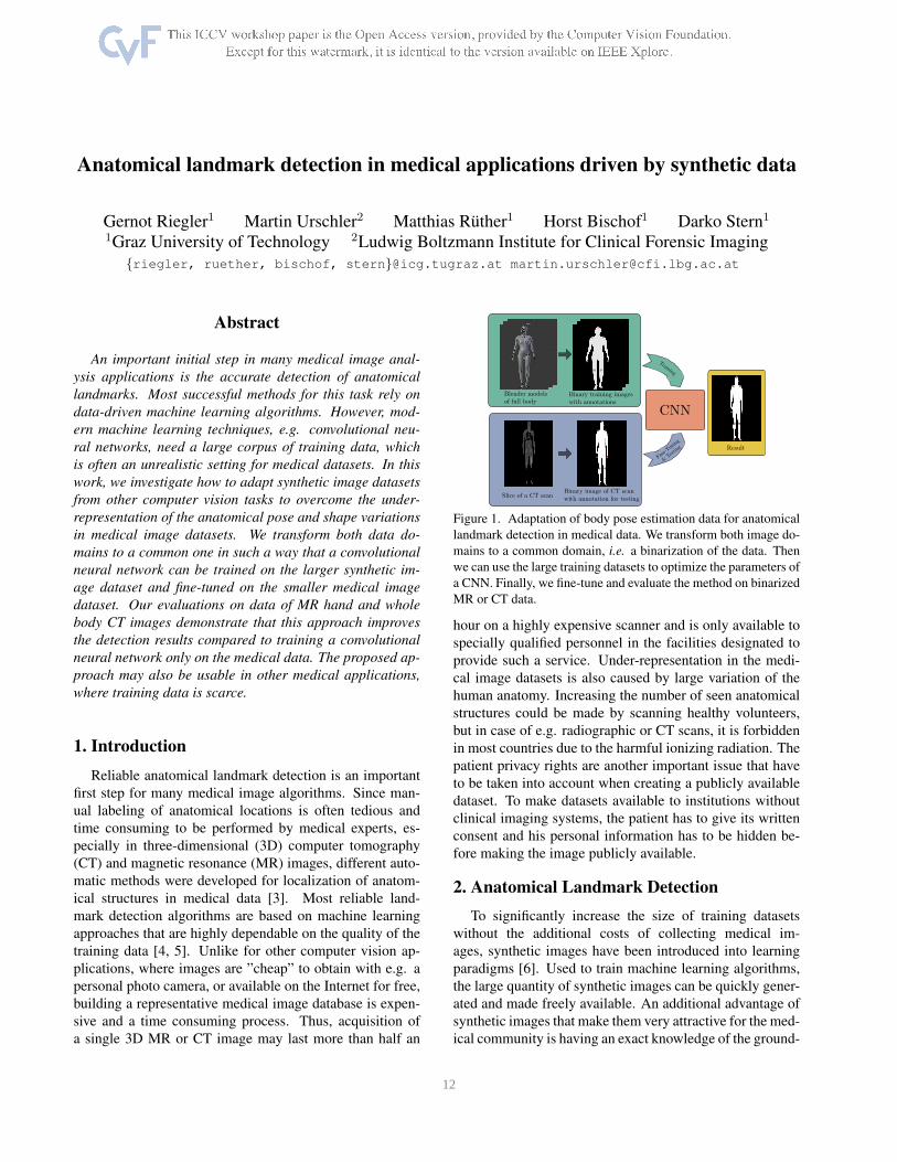
Figure 1. Adaptation of body pose estimation data for anatomical
landmark detection in medical data. We transform both image do-
mains to a common domain, i.e. a binarization of the data. Then
we can use the large training datasets to optimize the parameters of
a CNN. Finally, we fine-tune and evaluate the method on binarized
MR or CT data.
hour on a highly expensive scanner and is only available to
specially qualified personnel in the facilities designated to
provide such a service. Under-representation in the medi-
cal image datasets is also caused by large variation of the
human anatomy. Increasing the number of seen anatomical
structures could be made by scanning healthy volunteers,
but in case of e.g. radiographic or CT scans, it is forbidden
in most countries due to the harmful ionizing radiation. The
patient privacy rights are another important issue that have
to be taken into account when creating a publicly available
dataset. To make datasets available to institutions without
clinical imaging systems, the patient has to give its written
consent and his personal information has to be hidden be-
fore making the image publicly available.
2. Anatomical Landmark Detection
To significantly increase the size of training datasets
without the additional costs of collecting medical im-
ages, synthetic images have been introduced into learning
paradigms [6]. Used to train machine learning algorithms,
the large quantity of synthetic images can be quickly gener-
ated and made freely available. An additional advantage of
synthetic images that make them very attractive for the med-
ical community is having an exact knowledge of the ground-
1 12
Layer 1 Layer 2 Layer 3 Layer 4 Layer 5 Layer 6 Layer 7 Layer 8
conv5-32 maxpool2 conv5-32 maxpool2 conv3-32 fc2048 fc2048 fck
Table 1. Network architecture for anatomical landmark detection
for hand and whole body images. convw-c stands for a con-
volutional layer with filter size w × w and c output channels,
maxpoolp for max-pooling with pooling-width p, and fco for a
fully-connected layer with o outputs. The number of outputs in
the last layer depends on the number of anatomical landmarks.
truth positions of the represented structure. Nevertheless,
capturing the position and variation of under-investigated
anatomies, as well as its image intensity variation in dif-
ferent image modalities still remains the main challenge in
building realistic synthetic images.
When talking about detection of human or hand pose,
synthetic images have been successfully applied in com-
puter vision applications. In [18] and [19] the authors used
video-game images to train a holistic and a deformable part-
based model, respectively. Most famous is the work by
Shotton et al. [12], where the authors train a Random Forest
with a huge amount of synthetic and real training data for
the purpose of human pose estimation. Recently, such data-
driven approaches got also popular for articulated hand pose
estimation. Tang et al. [14] and Tompson et al. [16] utilized
a semi-automatic method to label a corpus of real depth-
sensor data to train their models. In contrast, Riegler et al.
[11] showed that convolution neural networks (CNN) [9]
can also successfully be trained on synthetic depth images
of the hand for articulated hand pose estimation.
The latter work was our inspiration to use synthetic im-
ages to overcome the limitation in the number of images,
especially labeled ones that are used in training an algo-
rithm for detection of body and hand pose in medical im-
ages. Similarly as in [11], we used a MakeHuman [1] model
and Blender [2] to generate a depth image training data set,
while casting the 3D medical image, such as MR or CT
data, to a depth image is straight forward. However, we can
further simplify the problem of mapping the different data
domains in training and testing by thresholding the image
data for both domains to obtain binary image data. With
this simple processing step, we can learn anatomical land-
mark estimators for medical images from synthetic data that
belong to a different training domain (see Fig. 1). Follow-
ing the idea in [20] we further adapt the trained CNN to the
medical image data set by performing a fine-tuning of the
network on a subset of the medical data.
2.1. Data Generation
The success of state-of-the-art CNN based approaches
for computer vision tasks depends on the depth of the CNN
(i.e. the number of layers) [13] and the amount of train-
ing data to avoid over-fitting. In the original work of [11]
a Blender model of a hand is articulated to sample from a
large space of different poses. For each pose a depth im-
age is rendered where the depth is measured relative to a
predefined camera and also the perfect ground-truth anno-
tation can be obtained in 3D. This avoids the cumbersome
and error-prone manual annotation process.
We modified the publicly available model in two ways to
fit our needs: First, we created new pose and shape spaces
for the anatomical landmark detection in hand and whole
body images. The key difference is that we need less varia-
tion in the articulation, but much more shape variation, es-
pecially for the whole body images. This is due to the fact
that the pose of the hand and body is relatively fixed dur-
ing a medical scan, but the shape of different people can
vary significantly, especially for the whole body scans (due
to differences in e.g. gender, weight and size). The sec-
ond modification to the model is the rendering itself, as we
render the binary image of the object along with the depth
image. We expect that the silhouette contains already suffi-
cient shape information for the detection of the anatomical
landmarks of interest in 2D. For the depth coordinate we
can train the regression model on a common depth domain,
as we will show in the experiments. Alternatively, we could
determine the depth information later with i.e. the mean po-
sition over the data set, because the depth coordinate varies
the least in 3D medical images In Fig. 1 we visualize one
example of our binary renderings for the whole body.
By marking the position in 2D binary image where im-
age intensity value is above the air threshold along the depth
direction of the 3D medical image, the 3D medical images
were mapped to the same domain as the 2D synthetic im-
ages in the training data set. Represented in 3D CT image
as two thin plates normal to the depth direction, CT scan-
ner tables were eliminated while generating the 2D binary
images by accumulating the number of high image intensity
values along the depth direction. Namely, the body in a 3D
CT image has more constant high intensity values than the
scanner table in the depth direction.
2.2. Inference Method
Provided with enough data, we can train a CNN for
anatomical landmark detection. We follow recent work in
body pose estimation [15, 17] and hand pose estimation
[11, 16] and formulate the task as a regression problem.
For each training image sn, we have an associated anno-
tation vector yn = (x1, y1, . . . , xk, yk)T that contains the k
ground-truth landmark locations. To aid generalization, we
scale the input image of the hand or whole body to a unit
size of ph × pw. Additionally, we also transform the anno-
tation vector similar to [17], such that the coordinates are in
the interval of [−1, 1]:
yp =
(
x1−
pw
2
pw
,y1−
ph
2
ph
, ...
)T
. (1)
We train a network φ with parameters w using stochas-
tic gradient descent with a mini-batch size of 100 that min-
2 13

thumb index middle ring pinky0
5
10
15
20
25
rmse [px]
footL footR kneeL kneeR handL handR shoulderL shoulderR head0
20
40
60
80
100
120
rmse [px]
method
NN(syn)
NN(CT)
RF
CNN(syn)
CNN(CT)
CNN(ft)
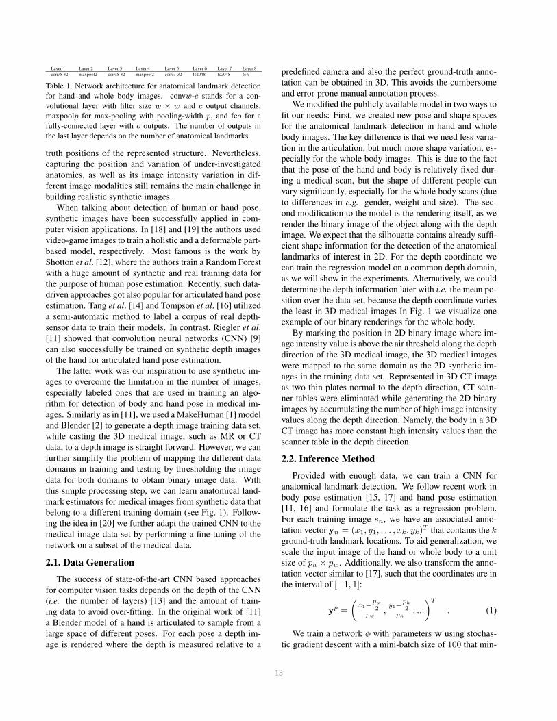
Figure 2. Anatomical landmark detection results on MR hand data (left) and CT scans of the whole body (right). We report the mean and
standard deviation of the root mean squared error (RMSE) between estimated and ground-truth anatomical landmark location in pixel (px).
The different colors depict the various methods.
imizes the L2 loss over the N training samples:
w = argminw
1
2
N∑
n=1
||φ(sn;w)− yPn ||
2 . (2)
The architecture of the network φ is listed in Table 1. We
use a ReLU [10] as activation after each convolutional and
fully-connected layer. Further, in the fully-connected layers
we use Dropout [8] to regularize the network.
Although we created the synthetic dataset with attention
to the pose variations in the MR data, we observed that fine-
tuning the model [7, 20] gives a significant performance im-
provement. Therefore, we use the small subset of binarized
MR/CT data to adapt the network weights to the original
domain, i.e. we use a new set of training data and re-train
the network on it. This follows the intuition that the syn-
thetic data is used to learn a rich feature representation and
the real data is used to re-parameterize the output space.
3. Experimental Set-Up
Datasets We evaluated our approach on two different
medical datasets, one of left hands from MR scans and one
of whole body CT scans. The left hand T1-weighted 3D
gradient echo MR images consists of scans from N = 132healthy male volunteers with an age between 13 and 24
years. The volunteers were asked to put their hand into the
MR scanner with slightly spread fingers and a half-kilo bag
of sand was placed on the top of their hand. In most of the
images, contraction of the fingers could be ignored, never-
theless the distances between the fingers, especially to the
thumb, varies among the volunteers. In the hand dataset,
five landmarks are located at the top the fingers.
The whole body dataset consists of N = 20 CT images
of cancer patients, of which 14 are female and 6 are male.
All patients are in a lying position with hands close to the
body and have slightly spread legs. Legs have the highest
variation in articulation and also the feet could be in an arbi-
trary position. The nine landmarks estimated in this dataset
are located at the top of the head, and at the left and right
shoulder, middle finger, knee and big toe, respectively.
Anatomical Landmark Detection of the Hand For the
landmark detection in MR images of the left hand we gen-
erated around 2.2M synthetic images. We scale the images
to a patch size of pw = ph = 96 and transform the annota-
tions accordingly such that they are in the range of [−1, 1].We train the network for 30 epochs with a learning rate
of 0.01 and a momentum term of 0.9. The learning rate
is decreased after each epoch by a factor of 0.7943. After
the training on the synthetic data, we fine-tune the network
on the binary MR images by performing a three-fold cross-
validation. Therefore, we train the network for 700 epochs
on this data (note that the number of training instances is
much smaller for fine-tuning). The learning rate and mo-
mentum term stay the same, but instead of a continuous de-
crease of the learning rate, we decrease the learning rate
once after 500 iterations by a factor of 0.1.
Anatomical Landmark Detection of the Whole Body
For the landmark detection in CT images of the whole body
we generated 600, 000 synthetic images, where the human
model varies in age, gender, size, body weight and pose. We
scale the images to a patch size with pw = 76, ph = 160and transform the annotations accordingly such that they are
in the range of [−1, 1].The network is also trained for 30 epochs with a learning
rate of 0.01 and a momentum term of 0.9. After each epoch
we decrease the learning rate by a factor of 0.7943. After
the training on the synthetic data, we again fine-tune the
network on the binarized CT data by performing a leave-
one-out cross-validation. Therefore, we train the network
for 700 epochs on 19 out of the 20 images and keep the
remaining one for testing. The learning rate and momentum
term stay the same, but instead a continuous decrease of the
learning rate, we decrease the learning rate once after 500iterations by a factor of 0.1.
Infer Depth of Anatomical Landmark Detections On
binarized input data one can only expect to determine the
2D location of anatomical landmarks. However, the vari-
ation in the depth coordinate can be expected to be rather
small, because the hand for example is always in the same
resting position when scanned in the MR. In fact, if we an-
alyze the depth of the individual landmarks for the hand
dataset, we observe a standard deviation from the mean
depth in the range from 3.137 voxels to 3.183 voxels for
the pinky and the thumb, respectively.
To refine these results, we can train a CNN on normal-
ized depth images, instead of binarized images. We nor-
malize the depth values of pixels that belong to the hand to
a zero mean and a unit standard deviation and set the back-
3 14
ground pixels to 3. In the same way we normalize the depth
annotation for the training samples. We do this for the syn-
thetic data to pre-train the CNN, as well as for the MR data
to fine-tune the network. The rest of the training follows the
same steps as described in the previous experiments.
4. Results and Discussion
The results of the MR hand landmark detection are de-
picted in Fig. 2. We compute for each landmark of the 263images the root mean squared error (rmse). The plot shows
the mean and standard deviation of each landmark for all
methods. We compare the fine-tuned network (CNN(ft)) to
the network trained solely on the synthetic data (CNN(syn))
and the binarized MR data (CNN(MR)). Further, we use a
nearest neighbor approach as baseline, where we compute
the location estimates by taking the mean annotation of the
three nearest patches. We denote the methods as NN(syn)
and NN(MR) if the nearest neighbour search is performed
on the synthetic data or the MR data, respectively. Finally,
we compare our method to the random regression forest RF
based state-of-the-art approach of [3].
First, we can observe that the NN(syn) approach per-
forms much worse than NN(MR). We assume that this is
due to the modeling of the synthetic data. Although we took
care to replicate the poses and shapes of the MR data, they
are still far off. The same explanation might hold for the
jump from CNN(syn) to CNN(ft). However, the fine-tuning
is still better than training the network on binary MR im-
ages only. The reason for the improvement is that the CNN
needs a lot of training data to tune all parameters, which
is performed with the synthetic data. The output parame-
ters are then adjusted with the fine-tuning of the network.
Finally, the method based on the random regression forest
[3] is inferior to the NN(MR), CNN(MR) and CNN(ft) meth-
ods. This is especially emphasized on the landmark with
the most variation, the thumb. Our explanation is that the
RF has the tendency to regress towards the mean anatomi-
cal landmark locations.
We visualize the results of the CT whole body cross-
validation in Fig. 2. The results are similar, but not as
pronounced as in the first evaluation. The NN(syn) is not
as good as the NN(CT). However, the NN(CT) fails for the
shoulder and head landmarks. This may be due to the small
dataset. What remains as an open question is why the RF
outperforms other approaches for the same three landmarks.
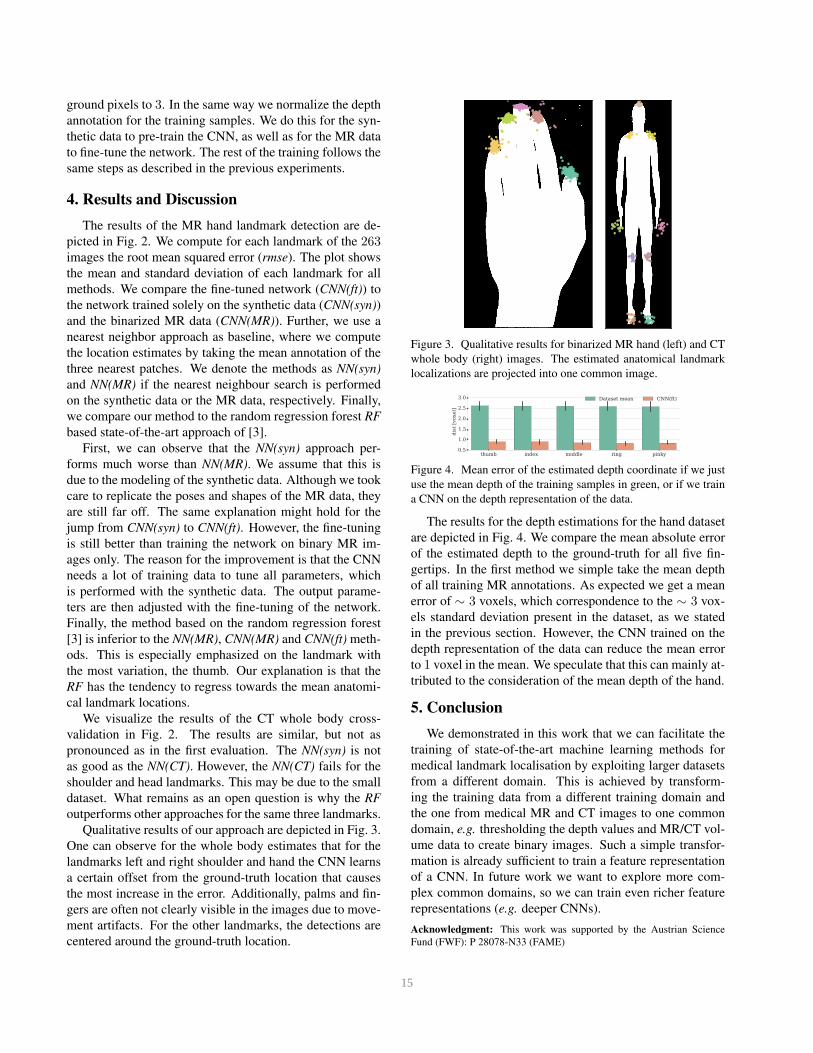
Qualitative results of our approach are depicted in Fig. 3.
One can observe for the whole body estimates that for the
landmarks left and right shoulder and hand the CNN learns
a certain offset from the ground-truth location that causes
the most increase in the error. Additionally, palms and fin-
gers are often not clearly visible in the images due to move-
ment artifacts. For the other landmarks, the detections are
centered around the ground-truth location.
Figure 3. Qualitative results for binarized MR hand (left) and CT
whole body (right) images. The estimated anatomical landmark
localizations are projected into one common image.
thumb index middle ring pinky0.5
1.0
1.5
2.0
2.5
3.0
dist [voxe
l]
Dataset mean CNN(ft)
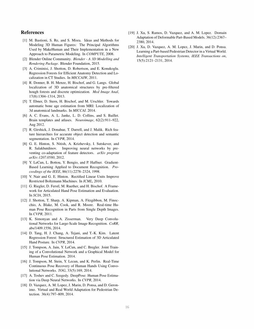
Figure 4. Mean error of the estimated depth coordinate if we just
use the mean depth of the training samples in green, or if we train
a CNN on the depth representation of the data.
The results for the depth estimations for the hand dataset
are depicted in Fig. 4. We compare the mean absolute error
of the estimated depth to the ground-truth for all five fin-
gertips. In the first method we simple take the mean depth
of all training MR annotations. As expected we get a mean
error of ∼ 3 voxels, which correspondence to the ∼ 3 vox-
els standard deviation present in the dataset, as we stated
in the previous section. However, the CNN trained on the
depth representation of the data can reduce the mean error
to 1 voxel in the mean. We speculate that this can mainly at-
tributed to the consideration of the mean depth of the hand.
5. Conclusion
We demonstrated in this work that we can facilitate the
training of state-of-the-art machine learning methods for
medical landmark localisation by exploiting larger datasets
from a different domain. This is achieved by transform-
ing the training data from a different training domain and
the one from medical MR and CT images to one common
domain, e.g. thresholding the depth values and MR/CT vol-
ume data to create binary images. Such a simple transfor-
mation is already sufficient to train a feature representation
of a CNN. In future work we want to explore more com-
plex common domains, so we can train even richer feature
representations (e.g. deeper CNNs).
Acknowledgment: This work was supported by the Austrian Science
Fund (FWF): P 28078-N33 (FAME)
4 15
References
[1] M. Bastioni, S. Re, and S. Misra. Ideas and Methods for
Modeling 3D Human Figures: The Principal Algorithms
Used by MakeHuman and Their Implementation in a New
Approach to Parametric Modeling. In COMPUTE, 2008.
[2] Blender Online Community. Blender - A 3D Modelling and
Rendering Package. Blender Foundation, 2015.
[3] A. Criminisi, J. Shotton, D. Robertson, and E. Konukoglu.
Regression Forests for Efficient Anatomy Detection and Lo-
calization in CT Studies. In MICCAIW, 2011.
[4] R. Donner, B. H. Menze, H. Bischof, and G. Langs. Global
localization of 3D anatomical structures by pre-filtered
hough forests and discrete optimization. Med Image Anal,
17(8):1304–1314, 2013.
[5] T. Ebner, D. Stern, H. Bischof, and M. Urschler. Towards
automatic bone age estimation from MRI: Localization of
3d anatomical landmarks. In MICCAI. 2014.
[6] A. C. Evans, A. L. Janke, L. D. Collins, and S. Baillet.
Brain templates and atlases. Neuroimage, 62(2):911–922,
Aug 2012.
[7] R. Girshick, J. Donahue, T. Darrell, and J. Malik. Rich fea-
ture hierarchies for accurate object detection and semantic
segmentation. In CVPR, 2014.
[8] G. E. Hinton, S. Nitish, A. Krizhevsky, I. Sutskever, and
R. Salakhutdinov. Improving neural networks by pre-
venting co-adaptation of feature detectors. arXiv preprint
arXiv:1207.0580, 2012.
[9] Y. LeCun, L. Bottou, Y. Bengio, and P. Haffner. Gradient-
Based Learning Applied to Document Recognition. Pro-
ceedings of the IEEE, 86(11):2278–2324, 1998.
[10] V. Nair and G. E. Hinton. Rectified Linear Units Improve
Restricted Boltzmann Machines. In ICML, 2010.
[11] G. Riegler, D. Ferstl, M. Ruether, and H. Bischof. A Frame-
work for Articulated Hand Pose Estimation and Evaluation.
In SCIA, 2015.
[12] J. Shotton, T. Sharp, A. Kipman, A. Fitzgibbon, M. Finoc-
chio, A. Blake, M. Cook, and R. Moore. Real-time Hu-
man Pose Recognition in Parts from Single Depth Images.
In CVPR, 2011.
[13] K. Simonyan and A. Zisserman. Very Deep Convolu-
tional Networks for Large-Scale Image Recognition. CoRR,
abs/1409.1556, 2014.
[14] D. Tang, H. J. Chang, A. Tejani, and T.-K. Kim. Latent
Regression Forest: Structured Estimation of 3D Articulated
Hand Posture. In CVPR, 2014.
[15] J. Tompson, A. Jain, Y. LeCun, and C. Bregler. Joint Train-
ing of a Convolutional Network and a Graphical Model for
Human Pose Estimation. 2014.
[16] J. Tompson, M. Stein, Y. Lecun, and K. Perlin. Real-Time
Continuous Pose Recovery of Human Hands Using Convo-
lutional Networks. TOG, 33(5):169, 2014.
[17] A. Toshev and C. Szegedy. DeepPose: Human Pose Estima-
tion via Deep Neural Networks. In CVPR, 2014.
[18] D. Vazquez, A. M. Lopez, J. Marin, D. Ponsa, and D. Geron-
imo. Virtual and Real World Adaptation for Pedestrian De-
tection. 36(4):797–809, 2014.
[19] J. Xu, S. Ramos, D. Vazquez, and A. M. Lopez. Domain
Adaptation of Deformable Part-Based Models. 36(12):2367–
2380, 2014.
[20] J. Xu, D. Vazquez, A. M. Lopez, J. Marin, and D. Ponsa.
Learning a Part-based Pedestrian Detector in a Virtual World.
Intelligent Transportation Systems, IEEE Transactions on,
15(5):2121–2131, 2014.
5 16


![Evaluation and Comparison of Anatomical Landmark Detection …hamarneh/ecopy/tmi2015b.pdf · 2015-05-04 · ization/identification of cephalometric landmarks [18]–[20]. In 2006,](https://img.dokumen.tips/doc/110x75/5ea4823bfa548e7f9520b73b/evaluation-and-comparison-of-anatomical-landmark-detection-hamarnehecopy-2015-05-04.jpg)