Robust Landmark Detection in Volumetric Data withEfficient 3D Deep Learning

Yefeng Zheng, David Liu, Bogdan Georgescu, Hien Nguyen, and Dorin Comaniciu

Medical Imaging Technologies, Siemens Healthcare, Princeton, NJ, USAyefeng.zheng@siemens.com

Abstract. Recently, deep learning has demonstrated great success in computervision with the capability to learn powerful image features from a large trainingset. However, most of the published work has been confined to solving 2D prob-lems, with a few limited exceptions that treated the 3D space as a compositionof 2D orthogonal planes. The challenge of 3D deep learning is due to a muchlarger input vector, compared to 2D, which dramatically increases the computa-tion time and the chance of over-fitting, especially when combined with limitedtraining samples (hundreds to thousands), typical for medical imaging applica-tions. To address this challenge, we propose an efficient and robust deep learningalgorithm capable of full 3D detection in volumetric data. A two-step approachis exploited for efficient detection. A shallow network (with one hidden layer)is used for the initial testing of all voxels to obtain a small number of promisingcandidates, followed by more accurate classification with a deep network. In addi-tion, we propose two approaches, i.e., separable filter decomposition and networksparsification, to speed up the evaluation of a network. To mitigate the over-fittingissue, thereby increasing detection robustness, we extract small 3D patches froma multi-resolution image pyramid. The deeply learned image features are furthercombined with Haar wavelet-like features to increase the detection accuracy. Theproposed method has been quantitatively evaluated for carotid artery bifurcationdetection on a head-neck CT dataset from 455 patients. Compared to the state-of-the-art, the mean error is reduced by more than half, from 5.97 mm to 2.64 mm,with a detection speed of less than 1 s/volume.

1 Introduction

An anatomical landmark is a biologically meaningful point on an organism, which canbe easily distinguished from surrounding tissues. Normally, it is consistently presentacross different instances of the same organism so that it can be used to establishanatomical correspondence within the population. There are many applications of au-tomatic anatomical landmark detection in medical image analysis. For example, land-marks can be used to align an input volume to a canonical plane on which physiciansroutinely perform diagnosis and quantification [1, 2]. A detected vascular landmarkprovides a seed point for automatic vessel centerline extraction and lumen segmen-tation [3, 4]. For a non-rigid object with large variation, a holistic detection may notbe robust. Aggregation of the detection results of multiple landmarks on the object mayprovide a more robust solution [5]. In some applications, the landmarks themselves pro-vide important measurements for disease quantification and surgical planning (e.g., the

1

distance from coronary ostia to the aortic hinge plane is a critical indicator whether thepatient is a good candidate for transcatheter aortic valve replacement [6]).

Various landmark detection methods have been proposed in the literature. Most ofthe state-of-the-art algorithms [1–6] apply machine learning (e.g., support vector ma-chines, random forests, or boosting algorithms) on a set of handcrafted image features(e.g., SIFT features or Haar wavelet-like features). However, in practice, we found somelandmark detection problems (e.g., carotid artery bifurcation landmarks in this work)are still too challenging to be solved with the current technology.

Deep learning [7] has demonstrated great success in computer vision with the capa-bility to learn powerful image features (either supervised or unsupervised) from a largetraining set. Recently, deep learning has been applied in many medical image anal-ysis problems, including body region recognition [8], cell detection [9], lymph nodedetection [10], organ detection/segmentation [11, 12], cross-modality registration [13],and 2D/3D registration [14]. On all these applications, deep learning outperforms thestate-of-the-art.

However, several challenges are still present in applying deep learning to 3D land-mark detection. Normally, the input to a neural network classifier is an image patch,which increases dramatically in size from 2D to 3D. For example, a patch of 32 × 32pixels generates an input of 1024 dimensions to the classifier. However, a 32× 32× 323D patch contains 32,768 voxels. Such a big input feature vector creates several chal-lenges. First, the computation time of a deep neural network is often too slow for areal clinical application. The most widely used and robust approach for object detec-tion is the sliding-window based approach, in which the trained classifier is tested oneach voxel in the volume. Evaluating a deep network on a large volume may take sev-eral minutes. Second, as a rule of thumb, a network with a bigger input vector requiresmore training data. With enough training samples (e.g., over 10 million in ImageNet),deep learning has demonstrated impressive performance gain over other methods. How-ever, the medical imaging community is often struggling with limited training samples(often in hundreds or thousands) due to the difficulty to generate and share images.Several approaches can tackle or at least mitigate the issue of limited training samples.One approach is to reduce the patch size. For example, if we reduce the patch size from32 × 32 × 32 voxels to 16 × 16 × 16, we can reduce the input dimension by a factorof eight. However, a small patch may not contain enough information for classifica-tion. Alternatively, instead of sampling a 3D patch, we can sample on three orthogonalplanes [15] or even a 2D patch with a random orientation [10]. Although they can ef-fectively reduce the input dimension, there is a concern on how much 3D informationis contained in 2D planes.

In this work we tackle the above challenges in the application of deep learning for3D anatomical structure detection (focusing on landmarks). Our approach significantlyaccelerates the detection speed, resulting in an efficient method that can detect a land-mark in less than one second. We apply a two-stage classification strategy (as shown inFig. 1). In the first stage, we train a shallow network with only one small hidden layer(e.g., with 64 hidden nodes). This network is applied to test all voxels in the volume in asliding-window process to generate 2000 candidates for the second stage classification.The second network is much bigger with three hidden layers (each has 2000 nodes)

2

DetectionResult

InputImage

Training Initial Detector with aShallow Network

Train Networkwith

SmoothnessConstraint

Approximationas 3D Separable

Filters

Training Bootstrapped Detector with a DeepNetwork

TrainNetwork with

L1-NormConstraint

NetworkSparsification

Run InitialDetector toGenerate

BootstrappedSamples

Layer-by-LayerPretraining withDenoising Auto

Encocder

Fig. 1. Training procedure of the proposed deep network based 3D landmark detection method.

to obtain more discriminative power. Such a cascaded classification approach has beenwidely used in object detection to improve detection efficiency and robustness.

In this work we propose two techniques to further accelerate the detection speed:separable filter approximation for the first-stage classifier and network sparsificationfor the second-stage classifier. The weights of a node in the first hidden layer are oftentreated as a filter (3D in this case). The response of the first hidden layer over the volumecan be calculated as a convolution with the filter. Here, a neighboring patch is shiftedby only one voxel; however, the response needs to be re-calculated from scratch. Inthis work we approximate the weights as separable filters using tensor decomposition.Therefore, a direct 3D convolution is decomposed as three one-dimensional convolu-tions along the x, y, and z axis, respectively. Previously, such approximation has beenexploited for 2D classification problems [16,17]. However, in 3D, the trained filters aremore difficult to be approximated as separable filters. We propose a new training costfunction to enforce smoothness of the filters so that they can be approximated with highaccuracy. The second big network only applies on a small number of candidates thathave little correlation. Separable filter approximation does not help to accelerate classi-fication. However, many weights in a big network are close to zero. We propose to addL1-norm regularization to the cost function to drive majority of the weights (e.g., 90%)to zero, resulting in a sparse network with increased classification efficiency withoutdeteriorating accuracy.

The power of deep learning is on the automatic learning of a hierarchical image rep-resentation (i.e., image features). Instead of using the trained network as a classifier, wecan use the responses at each layer (including the input layer, all hidden layers, and theoutput layer) as features and feed them into other state-of-the-art classifiers (e.g., boost-ing). After years of feature engineering, some handcrafted features have considerablediscriminative power for some applications and they may be complimentary to deeplylearned features. In this work we demonstrate that combining deeply learned featuresand Haar wavelet-like features, we can reduce the detection failures.

The remainder of this chapter is organized as follows. In Section 2 we present anew method to train a shallow network with separable filters, which are efficient in asliding-window based detection scheme to prune the landmark candidates. Section 3describes a sparse network that can effectively accelerate the evaluation of a deep net-work, which is used to further test the preserved landmark candidates. We present afeature fusion approach in Section 4 to combine Haar wavelet-like features and deeplylearned features to improve the landmark detection accuracy. Experiments on a large

3

dataset in Section 5 demonstrate the robustness and efficiency of the proposed method.This chapter concludes with Section 6. Please note, an early version of this work waspublished in [18].

2 Training Shallow Network with Separable Filters

A fully connected multilayer perceptron (MLP) neural network is a layered architecture.Suppose the input is a n0-dimensional vector [X0

1 , X02 , . . . , X

0n0]. The response of a

node X1j of the first hidden layer is

X1j = g

(n0∑i=1

W 0i,jX

0i + b0j

), (1)

for j = 1, 2, . . . , n1 (n1 is the number of nodes in the first hidden layer). Here, W 0i,j

is a weight; b0j is a bias term; And, g(.) is a nonlinear function, which can be sigmoid,hypo-tangent, restricted linear unit (ReLU), or other forms. In this work we use thesigmoid function

g(x) =1

1 + e−x, (2)

which is the most popular nonlinear function. If we denote X0 = [X01 , . . . , X

0n0]T and

W0j = [W 0

1,j , . . . ,W0n0,j

]T , Eq. (1) can be re-written as X1j = g

((W0

j )TX0 + b0j

).

Multiple layers can be stacked together using Eq. (1) as a building block. For a bi-nary classification problem as this work, the output of the network can be a singlenode X̂ . Suppose there are L hidden layers, the output of the neural network is X̂ =g((WL)TXL + bL

). During network training, we require the output to match the class

label Y (with 1 for the positive class and 0 for negative) by minimizing the squared errorE = ||Y − X̂||2.

In object detection using a sliding window based approach, for each position hy-pothesis, we crop an image patch (with a pre-defined size) centered at the positionhypothesis. We then serialize the patch intensities into a vector as the input to calculateresponse X̂ . After testing a patch, we shift the patch by one voxel (e.g., to the right)and repeat the above process again. Such a naive implementation is time consuming.Coming back to Eq. (1), we can treat the weights of a node in the first hidden layer asa filter. The first term of the response is a dot-product of the filter and the image patchintensities. Shifting the patch over the whole volume is equivalent to convolution usingthe filter. Therefore, alternatively, we can perform convolution using each filter W0

j forj = 1, 2, . . . , n1 and cache the response maps. During object detection, we can use thecached maps to retrieve the response of the first hidden layer.

Although such an alternative approach does not save computation time, it gives us ahint for speed-up. With a bit abuse of symbols, suppose Wx,y,z is a 3D filter with sizenx × ny × nz . Let’s further assume that Wx,y,z is separable, which means we can findthree one-dimensional vectors, Wx,Wy,Wz , such that

Wx,y,z(i, j, k) = Wx(i).Wy(j).Wz(k) (3)

4

for any i ∈ [1, nx], j ∈ [1, ny], and k ∈ [1, nz]. The convolution of the volume withWx,y,z is equivalent to three sequential convolutions with Wx, Wy , and Wz along itscorresponding axis. Sequential convolution with one-dimensional filters is much moreefficient than direct convolution with a 3D filter, especially for a large filter. However,in reality, Eq. (3) is just an approximation of filters learned by a neural network andsuch a rank-1 approximation is poor in general. In this work we search for S sets ofseparable filters to approximate the original filter as

Wx,y,z ≈S∑

s=1

Wsx.W

sy.W

sz. (4)

Please note, with a sufficient number of separable filters (e.g., S ≥ min{nx, ny, nz}),we can reconstruct the original filter perfectly.

To achieve detection efficiency, we need to cache n1 × S filtered response maps.If the input volume is big (the size of a typical CT scan in our dataset is about 300MB) and n1 is relatively large (e.g., 64 or more), the cached response maps consumea lot of memory. Fortunately, the learned filters W0

1, . . . ,W0n1

often have strong cor-relation (i.e., a filter can be reconstructed by a linear combination of other filters). Wedo not need to maintain a different filter bank for each W0

i . The separable filters inreconstruction can be drawn from the same bank,

W0i ≈

S∑s=1

ci,s.Wsx.W

sy.W

sz. (5)

Here, ci,s is the combination coefficient, which is specific for each filter W0i . However,

Wsx, Ws

y , and Wsz are shared by all filters. Eq. (5) is a rank-S decomposition of a 4D

tensor [W01,W

02, . . . ,W

0n1], which can be solved using [19].

Using 4D tensor decomposition, we only need to convolve the volume S times(instead of n1.S times using 3D tensor decomposition) and cache S response maps.Suppose the input volume has Nx × Ny × Nz voxels. For each voxel, we need to donxnynz multiplications using the original sliding window based approach. To calculatethe response of a hidden layer with n1 nodes, the total number of multiplications isn1nxnynzNxNyNz . Using the proposed approach, to perform convolution with S setof separable filters, we need do S(nx+ny+nz)NxNyNz multiplications. To calculatethe response of n1 hidden layer nodes, we need to combine the S responses usingEq. (5), resulting in n1SNxNyNz multiplications. The total number of multiplicationsis S(nx+ny +nz +n1)NxNyNz . Suppose S = 32, n1 = 64, the speed-up is 62 timesfor a 15× 15× 15 patch.

To achieve significant speed-up and save memory footprint, we need to reduce S asmuch as possible. However, we found, with a small S (e.g., 32), it was more difficult toapproximate 3D filters than 2D filters [16,17]. Non-linear functions g(.) are exploited inneural networks to bound the response to a certain range (e.g., [0, 1] using the sigmoidfunction). Many nodes are saturated (with an output close to 0 or 1) and once a node issaturated, its response is not sensitive to the change of the weights. Therefore, a weightcan take an extremely large value, resulting in a non-smooth filter. Here, we propose to

5

modify the objective function to encourage the network to generate smooth filters

E = ||Y − X̂||2 + α

n1∑i=1

||W0i −W0

i ||2. (6)

Here, W0i is the mean value of the weights of filter W0

i . So, the second term measuresthe variance of the filter weights. Parameter α (often takes a small value, e.g., 0.001)keeps a balance between two terms in the objective function. The proposed smoothregularization term is different to the widely used L2-norm regularization, which is asfollows

E = ||Y − X̂||2 + α

L∑j=1

nj∑i=1

||W0i ||2. (7)

The L2-norm regularization applies to all weights, while our regularization appliesonly to the first hidden layer. Furthermore, L2-norm regularization encourages smallweights, therefore shrinks the capacity of the network; while our regularization encour-ages small variance of the weights.

The training of the initial shallow network detector is as follows (as shown in theleft dashed box of Fig. 1). 1) Train a network using Eq. (6). 2) Approximate the learnedfilters using a filter bank with S (S = 32 in our experiments) sets of separable filtersto minimize the error of Eq. (5). The above process may be iterated a few times (e.g.,three times). In the first iteration, the network weights and filter bank are initialized withrandom values. However, in the following iterations, they are both initialized with theoptimal values from the previous iteration.

Previously, separable filter approximation has been exploited for 2D classificationproblems [16, 17]. We found 3D filters were more difficult to be approximated wellwith a small filter bank; therefore, we propose a new objective function to encouragethe network to generate smooth filters for higher separability. Furthermore, unlike [17],we also iteratively re-train the network to compensate the loss of accuracy due to ap-proximation.

3 Training Sparse Deep Network

Using a shallow network, we can efficiently test all voxels in the volume and assign adetection score to each voxel. After that, we preserve 2000 candidates with the largestdetection scores. The number of preserved candidates is tuned to have a high probabil-ity to include the correct detection (e.g., hypotheses within one-voxel distance to theground truth). However, most of the preserved candidates are still false positives. In thenext step, we train a deep network to further reduce the false positives. The classifica-tion problem is now much tougher and a shallow network does not work well. In thiswork we use a big network with three hidden layers, each with 2000 nodes.

Even though we only need to classify a small number of candidates, the computationmay still take some time since the network is now much bigger. Since the preservedcandidates are often scattered over the whole volume, separable filter decomposition asused in the initial detection stage does not help to accelerate the classification. After

6

checking the values of the learned weights of this deep network, we found most ofweights were very small, close to zero. That means many connections in the networkcan be removed without sacrificing classification accuracy. Here, we apply L1-normregularization to enforce sparse connection

E = ||Y − X̂||2 + β

L∑j=1

nj∑i=1

||Wji ||. (8)

Parameter β can be used to tune the number of zero weights. The higher β is, the moreweights converge to zero. With a sufficient number of training epochs, part of weightsconverges exactly to zero. In practice, to speed up the training, we periodically checkthe magnitude of weights. The weights with a magnitude smaller than a threshold areset to zero and the network is refined again. In our experiments, we find that 90% ofthe weigths can be set to zero after training, without deteriorating the classificationaccuracy. Thus, we can speed up the classification by roughly ten times.

The proposed acceleration technologies can be applied to different neural networkarchitectures, e.g., a multilayer perceptron (MLP) and a convolutional neural network(CNN). In this work we use the MLP. While the shallow network is trained with back-propagation to directly minimize the objective function in Eq. (6), the deep network ispre-trained using the denoising auto-encoder criterion [7] and then fine-tuned to mini-mize Eq. (8). The right dashed box of Fig. 1 shows the training procedure of the sparsedeep network.

4 Robust Detection by Combining Multiple Features

To train a robust neural network based landmark detector on limited training samples,we have to control the patch size. The optimal patch size was searched and we found asize of 15 × 15 × 15 achieved a good trade-off between detection speed and accuracy.However, a small patch has a limited field-of-view, thereby may not capture enoughinformation for classification. In this work we extract patches on an image pyramidwith multiple resolutions. A small patch in a low-resolution volume has a much largerfield-of-view at the original resolution. To be specific, we build an image pyramid withthree resolutions (1-mm, 2-mm, and 4-mm resolution, respectively). The intensities ofpatches from multiple resolutions are concatenated into a long vector to feed the net-work. As demonstrated in Section 5, a multi-resolution patch can improve the landmarkdetection accuracy.

Deep learning automatically learns a hierarchical representation of the input data.Representation at different hierarchical levels may provide complementary informa-tion for classification. Furthermore, through years’ of feature engineering, some hand-crafted image features can achieve quite reasonable performance on a certain task. Com-bining effective hand-crafted image features with deeply learned hierarchical featuresmay achieve even better performance than using them separately.

In this work we propose to use probabilistic boosting-tree (PBT) [20] to combineall features. A PBT is a combination of a decision tree and AdaBoost, by replacing aweak classification node in the decision tree with a strong AdaBoost classifier [21].

7

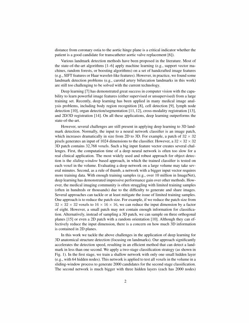
Table 1. Quantitative evaluation of carotid artery bifurcation detection accuracy on 455 CT scansbased on a four-fold cross validation. The errors are reported in millimeters.

Mean Std Median 80th PercentileHaar + PBT 5.97 6.99 3.64 7.84

Neural Network (Single Resolution) 4.13 9.39 1.24 2.35Neural Network (Multi-Resolution) 3.69 6.71 1.62 3.25

Network Features + PBT 3.54 8.40 1.25 2.31Haar + Network + PBT 2.64 4.98 1.21 2.39

Our feature pool is composed of two types of features: Haar wavelet-like features(h1, h2, . . . , hm) and neural network features rji (where rji is the response of node iat layer j). If j = 0, r0i is an input node, representing the image intensity of a voxel inthe patch. The last neural network feature is actually the response of the output node,which is the classification score by the network. This feature is the strongest feature andit is always the first selected feature by the AdaBoost algorithm.

Given 2000 landmark candidates generated by the first detection stage (Section 2),we evaluate them using the bootstrapped classifier presented in this section. We preserve250 candidates with the highest classification score and then aggregate them into asingle detection as follows. For each candidate we define a neighborhood, which is a8 × 8 × 8 mm3 box centered on the candidate. We calculate the total vote of eachcandidate as the summation of the classification score of all neighboring candidates.(The score of the current candidate is also counted since it is neighboring to itself.) Thecandidate with the largest vote is picked and the final landmark position is the weightedaverage (according to the classification score) of all candidates in its neighborhood.

5 Experiments

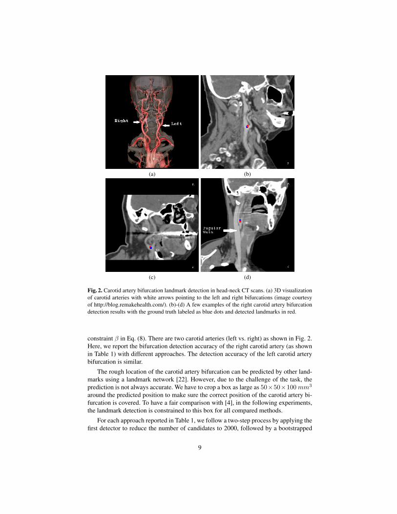
In this section we validate the proposed method on carotid artery bifurcation detection.The carotid artery is the main vessel supplying oxygenated blood to the head and neck.The common carotid artery originates from the aortic arch and runs up toward the headbefore bifurcating to the external carotid artery (supplying blood to face) and internalcarotid artery (supplying blood to brain). Examination of the carotid artery helps toassess the stroke risk of a patient. Automatic detection of this bifurcation landmarkprovides a seed point for centerline tracing and lumen segmentation, thereby makingautomatic examination possible. However, as shown in Fig. 2a, the internal/externalcarotid arteries further bifurcate to many branches and there are other vessels (e.g.,vertebral arteries and jugular veins) present nearby, which may cause confusion to anautomatic detection algorithm.

We collected a head-neck CT dataset from 455 patients. Each image slice has 512×512 pixels and a volume contains a variable number of slices (from 46 to 1181 slices).The volume resolution varies too, with a typical voxel size of 0.46× 0.46× 0.50mm3.To achieve a consistent resolution, we resample all input volumes to 1.0 mm. A four-fold cross validation is performed to evaluate the detection accuracy and determine thehyper parameters, e.g., the network size, smoothness constraint α in Eq. (6), sparsity

8

(a) (b)

(c) (d)

Fig. 2. Carotid artery bifurcation landmark detection in head-neck CT scans. (a) 3D visualizationof carotid arteries with white arrows pointing to the left and right bifurcations (image courtesyof http://blog.remakehealth.com/). (b)-(d) A few examples of the right carotid artery bifurcationdetection results with the ground truth labeled as blue dots and detected landmarks in red.

constraint β in Eq. (8). There are two carotid arteries (left vs. right) as shown in Fig. 2.Here, we report the bifurcation detection accuracy of the right carotid artery (as shownin Table 1) with different approaches. The detection accuracy of the left carotid arterybifurcation is similar.

The rough location of the carotid artery bifurcation can be predicted by other land-marks using a landmark network [22]. However, due to the challenge of the task, theprediction is not always accurate. We have to crop a box as large as 50×50×100mm3

around the predicted position to make sure the correct position of the carotid artery bi-furcation is covered. To have a fair comparison with [4], in the following experiments,the landmark detection is constrained to this box for all compared methods.

For each approach reported in Table 1, we follow a two-step process by applying thefirst detector to reduce the number of candidates to 2000, followed by a bootstrapped

9

detection to further reduce the number of candidates to 250. The final detection is pickedfrom the candidate with the largest vote from other candidates.

The value of a CT voxel represents the attenuation coefficient of the underlyingtissue to X-ray, which is often represented as a Hounsfield unit. The Hounsfield unithas a wide range from -1000 for air to 3000 for bones/metals and it is normally rep-resented with a 12-bit precision. A carotid artery filled with contrasted agent occupiesonly a small portion of the full Hounsfield unit range. Standard normalization meth-ods of neural network training (e.g., linear normalization to [0, 1] using the minimumand maximum value of the input, or normalizing to zero-mean and unit-variance) donot work well for this application. In this work we use a window based normalization.Intensities inside the window of [-24, 576] Hounsfield unit is linearly transformed to[0, 1]; Intensities less than -24 are truncated to 0; And, intensities higher than 576 aretruncated to 1.

Previously, Liu et al. [4] used Haar wavelet-like features + boosting to detect vascu-lar landmarks and achieved promising results. Applying this approach on our dataset,we achieve a mean error of 5.97 mm and the large mean error is caused by too manydetection outliers. The neural network based approach can significantly improve the de-tection accuracy with a mean error of 4.13 mm using a 15 × 15 × 15 patch extractedfrom a single resolution (1 mm). Using patches extracted from an image pyramid withthree resolutions, we can further reduce the mean detection error to 3.69 mm. If wecombine features from all layers of the network using the PBT, we achieve slightlybetter mean accuracy of 3.54 mm. Combining the deeply learned features and Haarwavelet-like features, we achieve the best detection accuracy with a mean error of 2.64mm. We suspect that the improvement comes from the complementary information ofthe Haar wavelet-like features and neural network features. Fig. 2 shows the detectionresults on a few typical datasets.

The proposed method is computationally efficient. Using the speed-up technologiespresented in Sections 2 and 3, it takes 0.92 s to detect a landmark on a computer witha six-core 2.6 GHz CPU (without using GPU). For comparison, the computation timeincreases to 18.0 s if we turn off the proposed acceleration technologies (namely, sep-arable filter approximation and network sparsification). The whole training proceduretakes about 6 hours and the sparse deep network consumes majority of the training time.

6 Conclusions

In this work we proposed 3D deep learning for efficient and robust landmark detec-tion in volumetric data. We proposed two technologies to speed up the detection usingneural networks, namely, separable filter decomposition and network sparsification. Toimprove the detection robustness, we exploit deeply learned image features trained ona multi-resolution image pyramid. Furthermore, we use the boosting technology to in-corporate deeply learned hierarchical features and Haar wavelet-like features to furtherimprove the detection accuracy. The proposed method is generic and can be re-trainedto detect other 3D landmarks or the center of organs.

10

References

1. Zhan, Y., Dewan, M., Harder, M., Krishnan, A., Zhou, X.S.: Robust automatic knee MR slicepositioning through redundant and hierarchical anatomy detection. IEEE Trans. MedicalImaging 30(12) (2011) 2087–2100

2. Schwing, A.G., Zheng, Y.: Reliable extraction of the mid-sagittal plane in 3D brain MRI viahierarchical landmark detection. In: Proc. Int’l Sym. Biomedical Imaging. (2014) 213–216

3. Zheng, Y., Tek, H., Funka-Lea, G., Zhou, S.K., Vega-Higuera, F., Comaniciu, D.: Efficientdetection of native and bypass coronary ostia in cardiac CT volumes: Anatomical vs. patho-logical structures. In: Proc. Int’l Conf. Medical Image Computing and Computer AssistedIntervention. (2011) 403–410

4. Liu, D., Zhou, S., Bernhardt, D., Comaniciu, D.: Vascular landmark detection in 3D CT data.In: Proc. of SPIE Medical Imaging. (2011) 1–7

5. Zheng, Y., Lu, X., Georgescu, B., Littmann, A., Mueller, E., Comaniciu, D.: Robust ob-ject detection using marginal space learning and ranking-based multi-detector aggregation:Application to automatic left ventricle detection in 2D MRI images. In: Proc. IEEE Conf.Computer Vision and Pattern Recognition. (2009) 1343–1350

6. Zheng, Y., John, M., Liao, R., Nottling, A., Boese, J., Kempfert, J., Walther, T., Brockmann,G., Comaniciu, D.: Automatic aorta segmentation and valve landmark detection in C-armCT for transcatheter aortic valve implantation. IEEE Trans. Medical Imaging 31(12) (2012)2307–2321

7. Vincent, P., Larochelle, H., Lajoie, I., Bengio, Y., Manzagol, P.A.: Stacked denoising autoen-coders: Learning useful representations in a deep network with a local denoising criterion.The Journal of Machine Learning Research 11 (2010) 3371–3408

8. Yan, Z., Zhan, Y., Peng, Z., Liao, S., Shinagawa, Y., Metaxas, D.N., Zhou, X.S.: Bodypartrecognition using multi-stage deep learning. In: Proc. Information Processing in MedicalImaging. (2015) 449–461

9. Liu, F., Yang, L.: A novel cell detection method using deep convolutional neural networkand maximum-weight independent set. In: Proc. Int’l Conf. Medical Image Computing andComputer Assisted Intervention. (2015) 349–357

10. Roth, H.R., Lu, L., Seff, A., Cherry, K.M., Hoffman, J., Wang, S., Liu, J., Turkbey, E., Sum-mers, R.M.: A new 2.5D representation for lymph node detection using random sets of deepconvolutional neural network observations. In: Proc. Int’l Conf. Medical Image Computingand Computer Assisted Intervention. (2014) 520–527

11. Carneiro, G., Nascimento, J.C., Freitas, A.: The segmentation of the left ventricle of the heartfrom ultrasound data using deep learning architectures and derivative-based search methods.IEEE Trans. Image Processing. 21(3) (2012) 968–982

12. Ghesu, F.C., Krubasik, E., Georgescu, B., Singh, V., Zheng, Y., Hornegger, J., Comaniciu,D.: Marginal space deep learning: Efficient architecture for volumetric image parsing. IEEETrans. Medical Imaging (2016)

13. Cheng, X., Zhang, L., Zheng, Y.: Deep similarity learning for multimodal medical images.Computer Methods in Biomechanics and Biomedical Engineering: Imaging & Visualization(2016) 1–5

14. Miao, S., Wang, Z.J., Zheng, Y., Liao, R.: Real-time 2D/3D registration via CNN regression.In: Proc. IEEE Int’l Sym. Biomedical Imaging. (2016) 1–4

15. Prasoon, A., Petersen, K., Igel, C., Lauze, F., Dam, E., Nielsen, M.: Deep feature learningfor knee cartilage segmentation using a triplanar convolutional neural network. In: Proc. Int’lConf. Medical Image Computing and Computer Assisted Intervention. Volume 8150. (2013)246–253

11

16. Rigamonti, R., Sironi, A., Lepetit, V., Fua, P.: Learning separable filters. In: Proc. IEEEConf. Computer Vision and Pattern Recognition. (2013) 2754–2761

17. Denton, E., Zaremba, W., Bruna, J., LeCun, Y., Fergus, R.: Exploiting linear structure withinconvolutional networks for efficient evaluation. In: Advances in Neural Information Process-ing Systems. (2014) 1–11

18. Zheng, Y., Liu, D., Georgescu, B., Nguyen, H., Comaniciu, D.: 3D deep learning for effi-cient and robust landmark detection in volumetric data. In: Proc. Int’l Conf. Medical ImageComputing and Computer Assisted Intervention. (2015) 565–572

19. Acar, E., Dunlavy, D.M., Kolda, T.G.: A scalable optimization approach for fitting canonicaltensor decompositions. Journal of Chemometrics 25(2) (2011) 67–86

20. Tu, Z.: Probabilistic boosting-tree: Learning discriminative methods for classification, recog-nition, and clustering. In: Proc. Int’l Conf. Computer Vision. (2005) 1589–1596

21. Freund, Y., Schapire, R.E.: A decision-theoretic generalization of on-line learning and anapplication to boosting. J. Computer and System Sciences 55(1) (1997) 119–139

22. Liu, D., Zhou, S., Bernhardt, D., Comaniciu, D.: Search strategies for multiple landmarkdetection by submodular maximization. In: Proc. IEEE Conf. Computer Vision and PatternRecognition. (2010) 2831–2838

12