Threshold and Complexity Results for the

Cover Pebbling Game

Anant P. Godbole (East Tennessee State Uni-

versity),

Nathaniel G. Watson (Washington University,

St. Louis),

and

Carl R. Yerger (Harvey Mudd College).

1

Given a connected graph G, distribute t peb-bles on its vertices in some configuration. Specif-ically, a configuration of weight t on a graphG is a function C from the vertex set V (G) toN ∪ {0} such that

∑v∈V (G) C(v) = t. Clearly C

represents an arrangement of pebbles on V (G).If the pebbles are indistinguishable, there are(n+t−1

t

)=(n+t−1

n−1

)configurations of t pebbles

on n vertices. Using quantum mechanical ter-minology as in Feller, we shall call this situ-ation Bose Einstein pebbling and posit thatthe underlying probability distribution is uni-form, i.e. that each of the

(n+t−1

n−1

)distrib-

utions are equally likely – should the pebblesbe thrown randomly onto the vertices. Thisis the model studied in Czygrinow et al. Nowthere is no reason to assume, a priori, thatthe pebbles are indistinguishable. Accordingly,if the pebbles are distinct, we shall refer toour process as Maxwell Boltzmann pebbling, inwhich a random distribution of pebbles leads tont equiprobable configurations. Maxwell Boltz-mann pebbling does not appear to have beenstudied more than peripherally in the literature.

2

A pebbling move is defined as the removal of

two pebbles from some vertex and the place-

ment of one of these on an adjacent vertex.

Given an initial configuration, a vertex v is

called reachable if it is possible to place a peb-

ble on it in finitely many pebbling moves. The

graph G is said to be pebbleable (this is not

standard nomenclature) if any of its vertices

can be thus reached. Define the pebbling num-

ber π(G) to be the minimum number of peb-

bles that are sufficient to pebble the graph re-

gardless of the initial configuration. The peb-

bling game may thus be described as follows:

Player 2 specifies a distribution C and a tar-

get vertex v. Player 1 wins the game iff she

is able to reach vertex v using a sequence of

pebbling moves. The pebbling number of G

is the smallest number t0 of pebbles so that

Player 1 wins no matter what strategy Player

2 employs.

3

The origin of pebbling is rather interesting and

somewhat unexpected. Time does not permit

us to share the underlying additive number the-

ory connection

SPECIAL CASES: The pebbling number π(Pn)

of the path is 2n−1. Chung proved that π(Qd) =

2d and π(Pmn ) = 2(n−1)m. An easy pigeonhole

principle argument yields π(Kn) = n. The peb-

bling number of trees has been determined (see

Hurlbert).

One of the key conjectures in pebbling, now

proved in several special cases, is due to Gra-

ham; its resolution would clearly generalize Chung’s

result for m-dimensional grids:

GRAHAM’S CONJECTURE.

π(G × H) ≤ π(G)π(H).

4

Structural characteristics of graphs have also

been employed to determine the pebbling num-

ber of specific classes of graphs. For instance,

a graph is said to be Class 0 if π(G) = |G|.Cubes are of Class 0, as are complete graphs,

but what other families fall in this important

class of graphs for which π is as low as it can

possibly be? Here are two answers: For graphs

of diameter 2, if G is 3-connected, then G is

Class 0 (Clark, Hurlbert and Hochberg). In

fact, they show that if we consider G(n, p), the

class of random graphs on n vertices where

the probability of each particular edge being

present is a fixed constant p ∈ (0,1), then al-

most all such graphs are Class 0. General-

izations of this result to the case where p =

pn → 0 as n → ∞ are also available. Other

authors, e.g. Chan and G, have obtained gen-

eral pebbling bounds, while Bukh has proved

almost-tight asymptotic bounds on the peb-

bling number of diameter three graphs.

5

In Random Pebbling, we seek the probability

that G is pebbleable when t pebbles are placed

randomly on it according to the B-E or M-

B scheme. Numerous threshold results have

been determined in Czygrinow at al. for B-E

pebbling of families of graphs such as Kn, the

complete graph on n vertices; Cn, the cycle

on n vertices; stars; wheels; etc. A threshold

result is a theorem of the following kind:

t = tn � an ⇒ P(G = Gn is pebbleable) → 1 (n → ∞)

t = tn � bn ⇒ P(G = Gn is pebbleable) → 0 (n → ∞),

Of course, we have reason to feel particularly

gratified if we can show that an = bn in a re-

sult of this genre. For the families of complete

graphs, wheels and stars, for example, we know

(Czygrinow et al.) that an = bn =√

n. In many

cases, however, the analysis is quite delicate;

see Wierman et al. for some of the issues in-

volved in finding the pebbling threshold for a

family as basic as Pn, the path on n vertices.

6

A detailed survey of graph pebbling has been

presented by Hurlbert, and it would probably

not be an oversimplification to state that most

results available to date fall in four broad cate-

gories: finding pebbling numbers for classes of

graphs; addressing the issue of when a family

of graphs is of class 0; pinpointing graph peb-

bling thresholds; and seeking to understand the

complexity issues in graph pebbling (Hulbert

and Kierstead). A survey of some not-open-

anymore problems in graph pebbling may be

found on Glenn Hurlbert’s website; see

http://math.la.asu.edu/∼hurlbert/HurlPebb.ppt

. The above mini-survey on pebbling notwith-

standing, we focus in this paper on a variant of

pebbling called cover pebbling, first discussed

by Crull et al. For reasons that will become

obvious, we focus only on analogs of the last

two of the four general directions mentioned

above.7

The cover pebbling number λ(G) is defined

as the minimum number of pebbles required

such that it is possible, given any initial con-

figuration of at least λ(G) pebbles on G, to

make a series of pebbling moves that simul-

taneously reaches each vertex of G. A con-

figuration is said to be cover solvable if it is

possible to place a pebble on every vertex of

G starting with that configuration. Various re-

sults on cover pebbling have been determined.

For instance, we now know (Crull et al.) that

λ(Kn) = 2n − 1;λ(Pn) = 2n − 1; and that for

trees Tn,

λ(Tn) = maxv∈V (Tn)

∑

u∈V (Tn)

2dist(u,v). (1)

Likewise, it was shown by Hurlbert and Munyon

that λ(Qd) = 3d and by Watson and Yerger

that λ(Kr1,...,rm) = 4r1 + 2r2 + . . . + 2rm − 3,

where r1 ≥ r2 ≥ . . . ≥ rm.

8

The above examples reveal that for these spe-

cial classes of graphs at any rate, the cover

pebbling number equals the “stacking num-

ber”, or, put another way, the worst possible

distribution of pebbles consists of placing all

the pebbles on a single vertex. The intuition

built by computing the value of the cover peb-

bling number for the families Kn, Pn, and Tn by

Crull et al. led to their Open Question No. 10,

which was christened the Stacking Conjecture

by students at the Summer 2004 East Ten-

nessee State University REU. In an exciting

summer development, participants Annalies Vuong

and Ian Wyckoff (paper submitted to EJC)

were able to prove the

STACKING THEOREM: For any connected

graph G,

λ(G) = maxv∈V (G)

∑

u∈V (G)

2dist(u,v),

9

thereby proving that (1) holds for all graphs.

In fact, the key result of Vuong and Wyck-

off is really a sufficient condition for a dis-

tribution to be cover solvable, so further in-

vestigations in the theory of (cover) pebbling

might soon veer, we speculate, in a fifth gen-

eral direction, namely a study of which dis-

tributions are (cover) solvable and which are

not. Finally, we mention that it is of great

interest that many of the 60+ authors who

have contributed to the theory of pebbling and

cover pebbling are undergraduates. The 2004

Mathfest featured talks by Aparna Higgins and

Zsuzsanna Szaniszlo that focused on contribu-

tions by undergraduates. Students at the Cen-

tral Michigan University, East Tennessee State

University, and University of Minnesota at Du-

luth REU sites, together with students at Val-

paraiso University and Arizona State Univer-

sity, have been among the key undergraduate

contributors.10

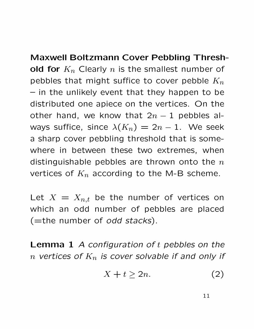
Maxwell Boltzmann Cover Pebbling Thresh-

old for Kn Clearly n is the smallest number of

pebbles that might suffice to cover pebble Kn

– in the unlikely event that they happen to be

distributed one apiece on the vertices. On the

other hand, we know that 2n − 1 pebbles al-

ways suffice, since λ(Kn) = 2n − 1. We seek

a sharp cover pebbling threshold that is some-

where in between these two extremes, when

distinguishable pebbles are thrown onto the n

vertices of Kn according to the M-B scheme.

Let X = Xn,t be the number of vertices on

which an odd number of pebbles are placed

(=the number of odd stacks).

Lemma 1 A configuration of t pebbles on the

n vertices of Kn is cover solvable if and only if

X + t ≥ 2n. (2)

11

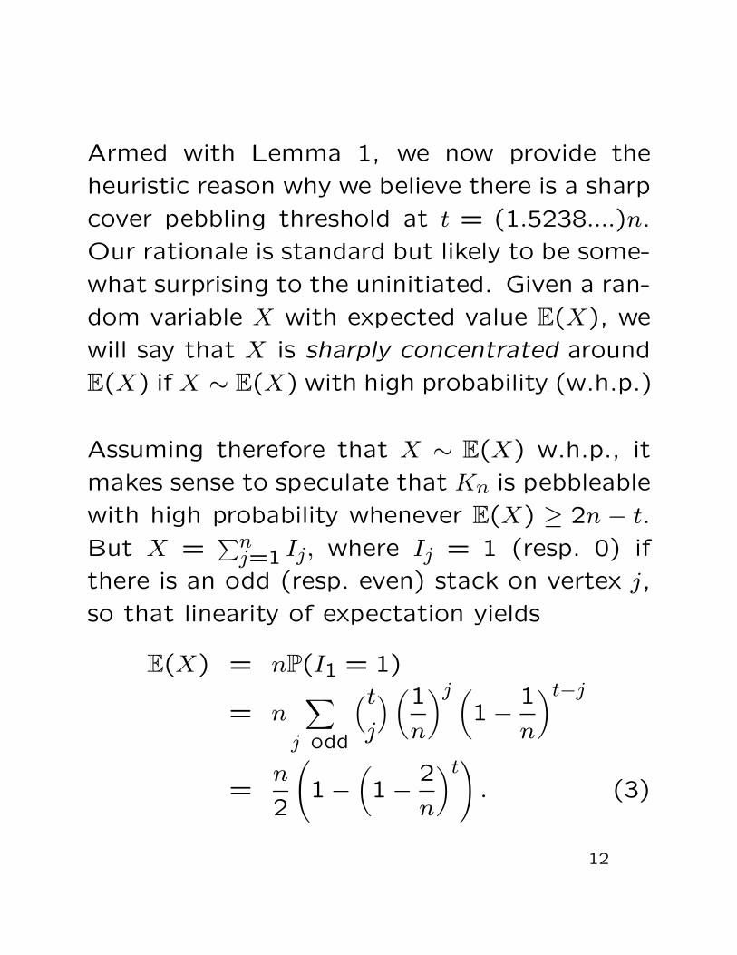
Armed with Lemma 1, we now provide the

heuristic reason why we believe there is a sharp

cover pebbling threshold at t = (1.5238....)n.

Our rationale is standard but likely to be some-

what surprising to the uninitiated. Given a ran-

dom variable X with expected value E(X), we

will say that X is sharply concentrated around

E(X) if X ∼ E(X) with high probability (w.h.p.)

Assuming therefore that X ∼ E(X) w.h.p., it

makes sense to speculate that Kn is pebbleable

with high probability whenever E(X) ≥ 2n − t.

But X =∑n

j=1 Ij, where Ij = 1 (resp. 0) if

there is an odd (resp. even) stack on vertex j,

so that linearity of expectation yields

E(X) = nP(I1 = 1)

= n∑

j odd

(tj

) (1

n

)j (1 −

1

n

)t−j

=n

2

(1 −

(1 −

2

n

)t)

. (3)

12

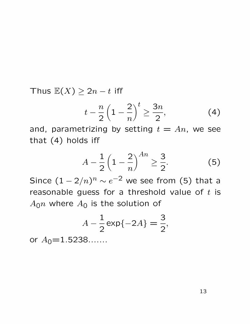
Thus E(X) ≥ 2n − t iff

t −n

2

(1 −

2

n

)t≥

3n

2, (4)

and, parametrizing by setting t = An, we see

that (4) holds iff

A −1

2

(1 −

2

n

)An≥

3

2. (5)

Since (1− 2/n)n ∼ e−2 we see from (5) that a

reasonable guess for a threshold value of t is

A0n where A0 is the solution of

A −1

2exp{−2A} =

3

2,

or A0=1.5238.......

13

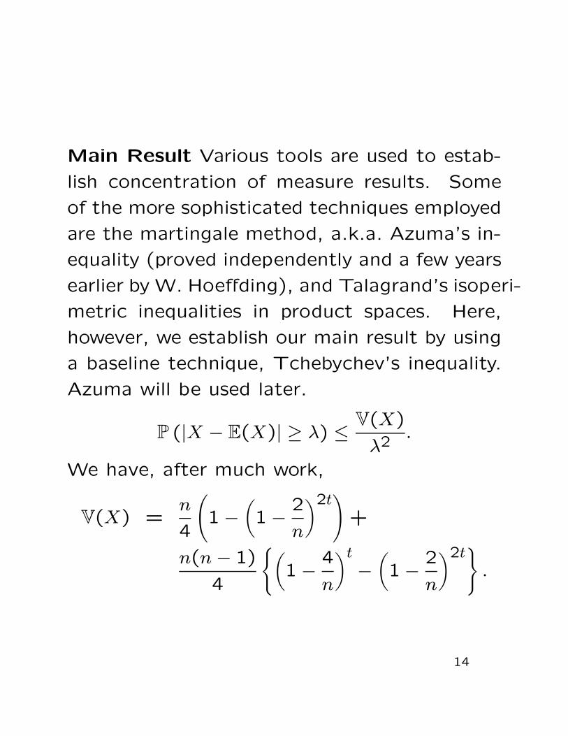
Main Result Various tools are used to estab-

lish concentration of measure results. Some

of the more sophisticated techniques employed

are the martingale method, a.k.a. Azuma’s in-

equality (proved independently and a few years

earlier by W. Hoeffding), and Talagrand’s isoperi-

metric inequalities in product spaces. Here,

however, we establish our main result by using

a baseline technique, Tchebychev’s inequality.

Azuma will be used later.

P (|X − E(X)| ≥ λ) ≤V(X)

λ2.

We have, after much work,

V(X) =n

4

(1 −

(1 −

2

n

)2t)

+

n(n − 1)

4

{(1 −

4

n

)t−(1 −

2

n

)2t}

.

14

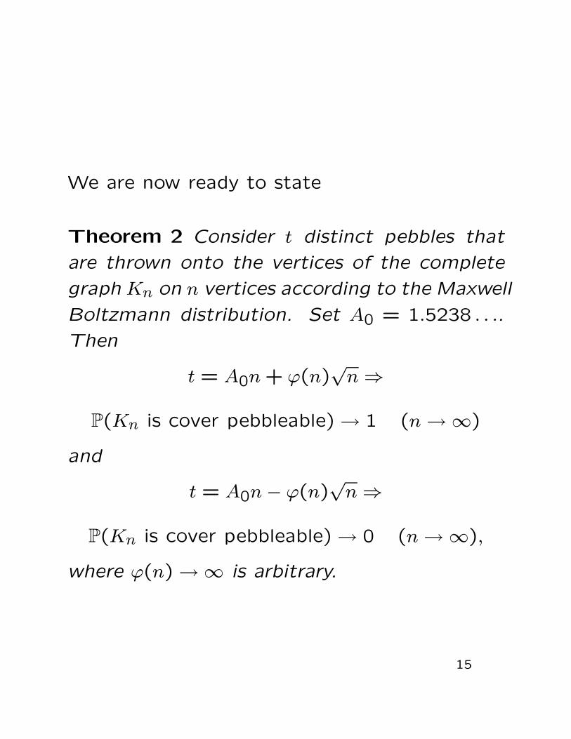
We are now ready to state

Theorem 2 Consider t distinct pebbles that

are thrown onto the vertices of the complete

graph Kn on n vertices according to the Maxwell

Boltzmann distribution. Set A0 = 1.5238 . . ..

Then

t = A0n + ϕ(n)√

n ⇒

P(Kn is cover pebbleable) → 1 (n → ∞)

and

t = A0n − ϕ(n)√

n ⇒

P(Kn is cover pebbleable) → 0 (n → ∞),

where ϕ(n) → ∞ is arbitrary.

15

Poissonization, Exchangeability, and the Questfor a Central Limit Theorem at the Thresh-old Theorem 2 raises a question. What is theprobability of being able to successfully coverpebble Kn at the threshold? Specifically, ift = A0n + B

√n for a constant B then what is

P(X ≥ 2n − t)?

One of the standard methods used in simplify-ing problems in discrete probability is that ofPoissonization. Given a random structure thatdepends on an input of fixed size, say t, westudy a related model in which the value ofthe input is random, specifically of size Po(t),where Po(λ) represents the Poisson randomvariable with parameter λ. In our case, wewill assign a Po(t) number of pebbles to then vertices of Kn, hoping that our results willreveal something meaningful about the situa-tion when the actual (as opposed to expected)number of pebbles is t. Returning to the fixedsize (or Bernoulli) model from the Poissonizedmodel is termed dePoissonization.

16

Specifically, we are interested in computing the

quantity

q(θ) =∑

sp(s)

e−θθs

s!,

where p(s) is the “real” object of interest (in

our case, the probability of cover pebbleability

when s pebbles are used). We hope, moreover,

in the spirit of Tauberian theorems, to recover

the p(s)s from their averages. Poissonization

has been studied in the context of “balls in

boxes” models by Aldous and by Holst, and

a heuristic is provided by Aldous that permits

one to dePoissonize:

A major study of analytic dePoissonization has

been conducted by Jacquet and Szpankowski,

and a serious application of their work is pro-

vided by Janson. The key result we use re-

quires that we traverse to the complex domain

to search for rigorous sufficient conditions that

permit dePoissonization:

17

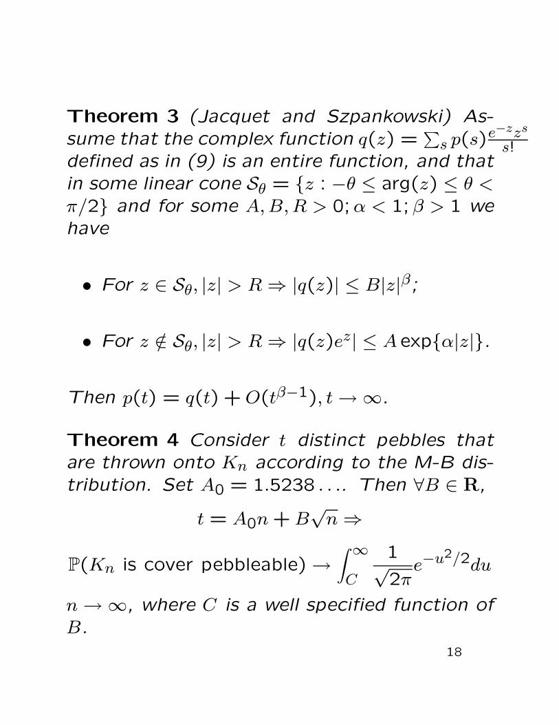
Theorem 3 (Jacquet and Szpankowski) As-sume that the complex function q(z) =

∑s p(s)e−zzs

s!defined as in (9) is an entire function, and thatin some linear cone Sθ = {z : −θ ≤ arg(z) ≤ θ <π/2} and for some A, B, R > 0;α < 1; β > 1 wehave

• For z ∈ Sθ, |z| > R ⇒ |q(z)| ≤ B|z|β;

• For z /∈ Sθ, |z| > R ⇒ |q(z)ez| ≤ A exp{α|z|}.

Then p(t) = q(t) + O(tβ−1), t → ∞.

Theorem 4 Consider t distinct pebbles thatare thrown onto Kn according to the M-B dis-tribution. Set A0 = 1.5238 . . .. Then ∀B ∈ R,

t = A0n + B√

n ⇒

P(Kn is cover pebbleable) →∫ ∞

C

1√2π

e−u2/2du

n → ∞, where C is a well specified function ofB.

18

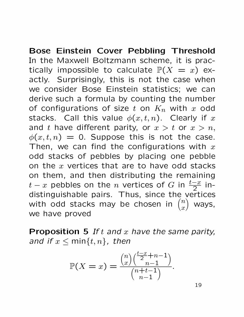
Bose Einstein Cover Pebbling ThresholdIn the Maxwell Boltzmann scheme, it is prac-tically impossible to calculate P(X = x) ex-actly. Surprisingly, this is not the case whenwe consider Bose Einstein statistics; we canderive such a formula by counting the numberof configurations of size t on Kn with x oddstacks. Call this value φ(x, t, n). Clearly if xand t have different parity, or x > t or x > n,φ(x, t, n) = 0. Suppose this is not the case.Then, we can find the configurations with xodd stacks of pebbles by placing one pebbleon the x vertices that are to have odd stackson them, and then distributing the remainingt − x pebbles on the n vertices of G in t−x

2 in-distinguishable pairs. Thus, since the verticeswith odd stacks may be chosen in

(nx

)ways,

we have proved

Proposition 5 If t and x have the same parity,and if x ≤ min{t, n}, then

P(X = x) =

(nx

)(t−x2 +n−1

n−1

)

(n+t−1

n−1

) .

19

Polya Sampling and Azuma’s Inequality Yield

Dividends There is a natural and sequentialprobabilistic process associated with MaxwellBoltzmann pebbling. We simply take t pebbles(balls) and throw them one by one onto (into)n vertices (urns) in the “natural” way that in-spires many elementary problems in discreteprobability texts. By contrast, the “global”Bose-Einsteinian positioning of t indistinct ballsinto n distinct urns – so that we obtain

(n+t−1

n−1

)

equiprobable configurations – does not appearto have a sequential process associated with it.But it does. We first rephrase the problem –not as one associated with throwing balls intoboxes but, conversely, as a sampling problem,i.e., drawing balls from boxes. In this light,Maxwell Boltzmann pebbling consists of draw-ing t balls “with replacement” from a box con-taining one ball of each of n colors, with theunderstanding that the number of balls of colorj drawn in the altered model equals the num-ber of pebbles that are tossed onto vertex j

20

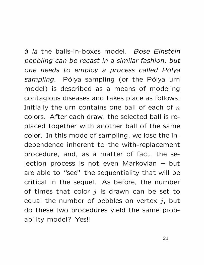
a la the balls-in-boxes model. Bose Einstein

pebbling can be recast in a similar fashion, but

one needs to employ a process called Polya

sampling. Polya sampling (or the Polya urn

model) is described as a means of modeling

contagious diseases and takes place as follows:

Initially the urn contains one ball of each of n

colors. After each draw, the selected ball is re-

placed together with another ball of the same

color. In this mode of sampling, we lose the in-

dependence inherent to the with-replacement

procedure, and, as a matter of fact, the se-

lection process is not even Markovian – but

are able to “see” the sequentiality that will be

critical in the sequel. As before, the number

of times that color j is drawn can be set to

equal the number of pebbles on vertex j, but

do these two procedures yield the same prob-

ability model? Yes!!

21

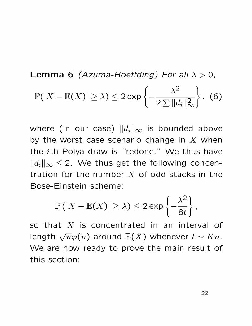
Lemma 6 (Azuma-Hoeffding) For all λ > 0,

P(|X − E(X)| ≥ λ) ≤ 2 exp

{−

λ2

2∑

‖di‖2∞

}. (6)

where (in our case) ‖di‖∞ is bounded above

by the worst case scenario change in X when

the ith Polya draw is “redone.” We thus have

‖di‖∞ ≤ 2. We thus get the following concen-

tration for the number X of odd stacks in the

Bose-Einstein scheme:

P (|X − E(X)| ≥ λ) ≤ 2exp

{−

λ2

8t

},

so that X is concentrated in an interval of

length√

nϕ(n) around E(X) whenever t ∼ Kn.

We are now ready to prove the main result of

this section:

22

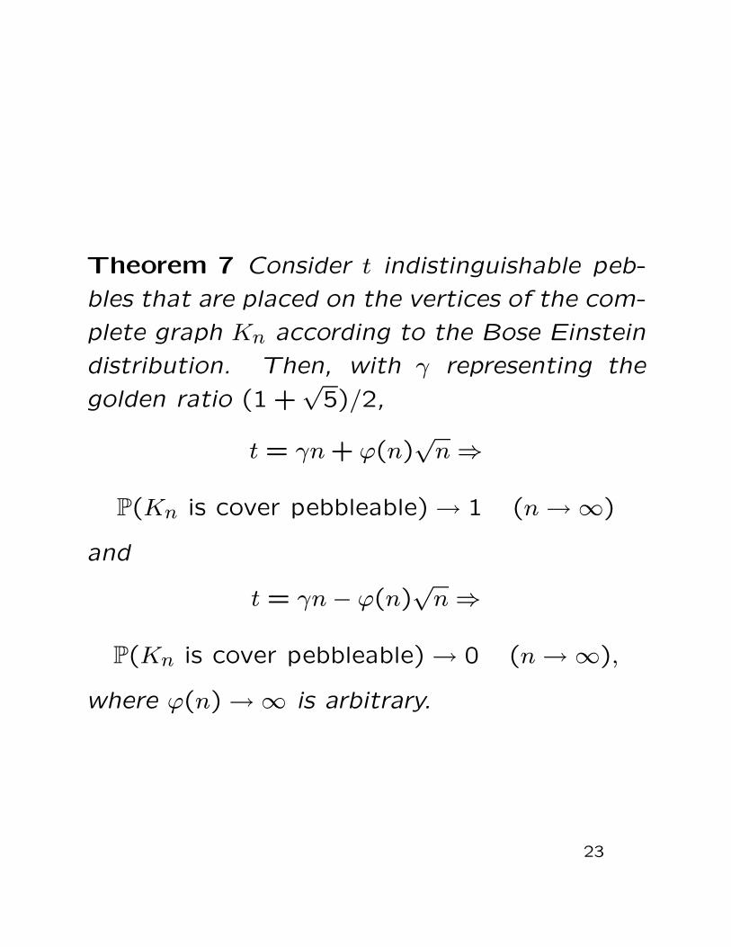
Theorem 7 Consider t indistinguishable peb-

bles that are placed on the vertices of the com-

plete graph Kn according to the Bose Einstein

distribution. Then, with γ representing the

golden ratio (1 +√

5)/2,

t = γn + ϕ(n)√

n ⇒

P(Kn is cover pebbleable) → 1 (n → ∞)

and

t = γn − ϕ(n)√

n ⇒

P(Kn is cover pebbleable) → 0 (n → ∞),

where ϕ(n) → ∞ is arbitrary.

23

NP-Completeness of the Cover Pebbling

Problem One of the obvious open problems

that can be formulated as a result of our work

is the following: What are cover pebbling thresh-

olds for families of graphs other than Kn? It

would certainly advance the theory of cover

pebbling if one could uncover a host of results

similar, e.g. to Theorems 2 and 10. Such re-

sults would provide a nice complement to those

by Hurlbert and Kierstead. Our results in this

section show, however, that this task might

not be as easy as one might imagine. Nec-

essary and sufficient conditions for the cover

pebbleability of a graph are likely to be compli-

cated, and the best hope might thus be to es-

tablish necessary conditions and sufficient con-

ditions that are not too far apart.

24

Theorem 8 Let G be a graph, C a configura-

tion on G. Let |G| = m and label the vertices

of G as v1, v2, . . . vm Then C is cover solvable

if and only if there exist integers nij ≥ 0 with

1 ≤ i, j ≤ m and nij = 0 and nji = 0 whenever

{vi, vj} /∈ E(G) such that for all 0 ≤ k ≤ m,

C(vk) +m∑

l=1

nlk − 2m∑

l=1

nkl ≥ 1.

Corollary 9 The cover solvability decision prob-

lem which accepts pairs {G, C} if and only if G

is a graph and C is a configuration which is

cover solvable on G is in NP.

25

Now we turn our attention to showing that the

cover solvability decision problem is NP -hard,

that is, that any instance of any problem in NP

can be translated to an instance of cover solv-

ability in polynomial time. The usual method

of showing that a problem A is NP -hard is to

find an NP -complete problem B for which any

instance of B can be translated into an in-

stance of A in polynomial time. Then for any

instance of any problem in NP we can translate

it in polynomial time to an instance of B, then

translate this instance into an instance of A.

For cover solvability, we will use a known NP -

complete problem known as “exact cover by

4-sets.” Indeed, the corresponding and seem-

ingly simpler problem of perfect cover by 3-sets

is also NP -complete, but for our purposes, the

4-set problem is more useful.

26

Theorem 10 Let the exact cover by 4-sets

problem be the decision problem which takes

as input a set S with 4n elements and a class

A of at least n four-element subsets of S, ac-

cepting such a pair if there exists an A′ ⊆ A

such that A′ is a class of disjoint subsets which

make a partition of S, that is they are n subsets

containing every element of S. This problem is

NP -complete

Theorem 11 The cover solvability decision prob-

lem is NP -complete

27