Embed Size (px)
Citation preview

Saarland University
Faculty of Natural Sciences and Technology IDepartment of Computer Science
Master’s Thesis
An Analysis
of Automatic Chord Recognition Procedures
for Music Recordings
submitted by
Nanzhu Jiang
submitted
February 4, 2011
Supervisor / Advisor
Priv.-Doz. Dr. Meinard Muller
Reviewers
Priv.-Doz. Dr. Meinard Muller
Prof. Dr. Michael Clausen

Eidesstattliche Erklarung
Ich erklare hiermit an Eides Statt, dass ich die vorliegende Arbeit selbststandig verfasstund keine anderen als die angegebenen Quellen und Hilfsmittel verwendet habe.
Statement under Oath
I confirm under oath that I have written this thesis on my own and that I have not usedany other media or materials than the ones referred to in this thesis.
Einverstandniserklarung
Ich bin damit einverstanden, dass meine (bestandene) Arbeit in beiden Versionen in dieBibliothek der Informatik aufgenommen und damit veroffentlicht wird.
Declaration of Consent
I agree to make both versions of my thesis (with a passing grade) accessible to the publicby having them added to the library of the Computer Science Department.
Saarbrucken,(Datum / Date) (Unterschrift / Signature)

Acknowledgements
First of all, I am thankful to my supervisor from the bottom of my heart, Meinard Muller,whose excellent guidance, support and patience have always inspired me to work on thisthesis. Furthermore, it is him who opens the door of music processing to me and let mefind my real interest during my master studies.
I would like to express my deepest gratitude to Peter Grosche. He has made valuablesupports in a number of ways such as the suggestions and discussions about problems,patiently helping me to arrange figures and tables of the thesis. His passionate attitudetowards research also encouraged me when I get frustrated at the difficulties.
This thesis would not have been possible without the help of Verena Konz. She hasprecisely labeled the pieces of music which are of great importance for me. I am gratefulfor all her supports from the beginning of my thesis to the end. I would like to expressthe gratitude to her for the many music knowledge she explained as well as many manyuseful information about daily life.
I am indebted to many of my friends who support me during the writing of my thesis.Thomas Pratzlich, Philipp von StypRekowsky, Zhe Zuo, Haichao Guan, Jing Cui, YuanGao, Yecheng Gu and Qian Ma have all helped to proofread my thesis. They have givenme the detailed and helpful feedback. I am grateful for their help. In particular, some ofthem were quite busy with their own work, however they still took their time for correctingmy errors and offered suggestions.
I would like to specially thank Shuyan Liu and Shujie Li, for always supporting me duringthe whole period of my thesis. I can still remember the depressed time when I wasfrustrated by so many things messed up together, it is them who always stay beside meand cheer me up.
Finally, many thanks to my dear parents. Thanks for their unlimited love and care.Thanks very much for their understanding and let me pursue my dream so long and sofar away from home.

Abstract
Chord recognition task is to split up a piece of music into segments and assign each ofthem a chord label according to the analysis of the harmonic content. Making the chordrecognition task process audio recordings automatically will be of great help for musicinformation retrieval. Most of the existing chord recognition systems proceed as follows.In the first step, a given audio recording is converted into a sequence of chroma features. Inthe second step, the feature sequence is passed into chord recognition module in which thefeatures are assigned with chord labels. However, although much research has been done,there is little understanding of the effect of the different processing stages and of the variousparameter settings on the final recognition result. In this thesis we analyze the differentstages of typical automated chord recognition systems. In particular, we consider severaltypes of chroma features as well as several chord recognition methods based on simpletemplates and more statistical involved pattern matching. As the main contribution, weconduct extensive experiments to evaluate the impact of different modules. In particular,we investigate the role of the parameters from both the feature side and the recognizerside systematically to reveal how they influence the overall performance. Our aim is tobetter understand the effect of different stages and their interaction as well as to indicatedirections towards potential improvements. Finally, we add some additional processingtechniques such as detuning compensation, harmonic-percussive source separation andbeat-synchronization, and briefly examine their influence on chord recognition results.

iv

Contents
1 Introduction 1
1.1 Music Background . . . . . . . . . . . . . . . . . . . . . . . . . . . . . . . . 11.2 Chord Recognition Task . . . . . . . . . . . . . . . . . . . . . . . . . . . . . 41.3 System Framework . . . . . . . . . . . . . . . . . . . . . . . . . . . . . . . . 4
1.4 Mathematical Formulation . . . . . . . . . . . . . . . . . . . . . . . . . . . . 71.5 Contribution . . . . . . . . . . . . . . . . . . . . . . . . . . . . . . . . . . . 71.6 Organization of Thesis . . . . . . . . . . . . . . . . . . . . . . . . . . . . . . 7
2 Feature Extraction 11
2.1 Pitch Features . . . . . . . . . . . . . . . . . . . . . . . . . . . . . . . . . . 122.2 Chroma Features . . . . . . . . . . . . . . . . . . . . . . . . . . . . . . . . . 142.3 Chroma Features with Logarithmic Compression . . . . . . . . . . . . . . . 172.4 CENS Features . . . . . . . . . . . . . . . . . . . . . . . . . . . . . . . . . . 18
2.5 CRP Features . . . . . . . . . . . . . . . . . . . . . . . . . . . . . . . . . . . 202.6 CISP Features . . . . . . . . . . . . . . . . . . . . . . . . . . . . . . . . . . 21
3 Template-based Chord Recognition 23
3.1 Template-based Chord Recognition . . . . . . . . . . . . . . . . . . . . . . . 23
3.2 Specification of Chord Template Sets . . . . . . . . . . . . . . . . . . . . . . 243.3 Specification of Distance Measures . . . . . . . . . . . . . . . . . . . . . . . 323.4 Template Method Summary . . . . . . . . . . . . . . . . . . . . . . . . . . . 32
4 Statistical Model-based Chord Recognition 35
4.1 Multivariate Gaussian Distribution . . . . . . . . . . . . . . . . . . . . . . . 364.2 Specification of the Chord Models . . . . . . . . . . . . . . . . . . . . . . . 394.3 Mahalanobis Distance based-Method . . . . . . . . . . . . . . . . . . . . . . 40
4.4 Gaussian Probability based-Method . . . . . . . . . . . . . . . . . . . . . . 424.5 Hidden Markov Models-based Method . . . . . . . . . . . . . . . . . . . . . 43
5 Experiments 47
5.1 Experiments Setup . . . . . . . . . . . . . . . . . . . . . . . . . . . . . . . . 47
5.2 Evaluation via Precision and Recall . . . . . . . . . . . . . . . . . . . . . . . 495.3 Experiments on Extracted Features . . . . . . . . . . . . . . . . . . . . . . . 495.4 Experiments on Chord Recognition Methods . . . . . . . . . . . . . . . . . 625.5 Effect of Tuning . . . . . . . . . . . . . . . . . . . . . . . . . . . . . . . . . 71
5.6 Effect of Using Different Training Datasets . . . . . . . . . . . . . . . . . . 725.7 Harmonic Percussive Source Separation . . . . . . . . . . . . . . . . . . . . 73
v

vi CONTENTS
5.8 Effect of Using Beat Synchronized Feature . . . . . . . . . . . . . . . . . . . 755.9 Experiments on Classical Dataset . . . . . . . . . . . . . . . . . . . . . . . . 76
6 Summary 79
A Source Code 81
List of Figures 87
List of Tables 89

Chapter 1
Introduction
1.1 Music Background
A chord is defined as the simultaneous sounding of two or more different notes [21]. Nor-mally the notes which form the chord are played together just like a musician pressesthe corresponding keys at the same time. In some special cases, these notes are playedseparately yet successively as a musician press the key one by one. Such cases includearpeggios and broken chords. Figure 1.1 illustrates a chord with the notes played simulta-neously and Figure 1.1(b) illustrates the arpeggio, where the notes are played separately.Chords themselves and their progression are very important because they compose theharmonic content of a music piece. The analysis of harmonic content is essential in theWestern tonal music, thus chords as the fundamental component play a crucial role forthe understanding of such music [29]. Furthermore, being a higher-level representationof a music piece compared to the note-level representation, chords bring more insight tothe analysis of the music structure and therefore assist many music information retrievalapplications such as cover song identification and music segmentation.
(a) (b)
Figure 1.1. (a) C major triad played simultaneously, (b) C major triad in arpeggio.
By looking at the number of distinct notes1 which compose a chord, we categorize thechords as “triad”, “seventh”, “ninth”, etc. Figure 1.2 illustrates a triad, seventh andninth chord based on the root note C. The most commonly used chords in music pieces
1Here, distinct notes means the notes which are in different pitch classes. For the definition of pitchclass, see chapter 2
1

2 CHAPTER 1. INTRODUCTION
are “triad” chords. The name “triad” indicates that such chord is composed by threedistinct notes. However, since notes which in different octave yet in the same pitch classmay be considered as one note when people analyze the chord, it is better to count thenumber of distinct “pitch classes” or “chromas” instead of distinct notes. Figure 1.3illustrates how notes are mapped to chroma2. To avoid confusion, in this thesis when wemention a component note of a chord, we actually treat all the notes in a pitch class asone note disregarding their octave information.
Figure 1.2. Three types of chords with different number of notes based on root note C. From leftto right: C major triad, C dominant seventh and C major ninth.
(a) (b)
Figure 1.3. (a) Chromatic circle. (b) Shepards helix of pitch perception [2].
The component notes of a chord are not randomly selected but chosen according to themusical interval. It is the musical distance between the pitches of simultaneously soundingnotes. The chords can be classified in this way as “major”, “minor”, “augmented”, “di-minished” indicating the component notes of these chords have different intervals. Figure1.4 illustrate these four kind of chords with different intervals. Moreover, every compo-nent note has its own name closely related to the intervals. Taking the major triad3 asan example, the lowest note is called root note, and the musical intervals of all other com-ponent notes are based on this note; the highest note is called fifth meaning it has a fifthinterval from the root note; the middle note is called the third meaning it has a majorthird interval from the root. For the case of a minor triad, the lowest and highest noteare the same for the major triad, the only difference lies in the middle note: this time itis the note which has a minor third interval.
Another essential concept about chords is the inversions. The concept of a chord inversionsis introduced due to such cases that the root note of a chord is not at the lowest position,but somewhere higher. Figure 1.5 shows the three variations of C major triad, with the
2Figure 1.3 (a) is reproduced from http://en.wikipedia.org/wiki/Chromatic_circle3Here we mean the major triad is in root position.

1.1. MUSIC BACKGROUND 3
Figure 1.4. Chords with different musical intervals based on the root note C. From left to right:C major triad, C minor triad, C augmented triad and C diminished triad.
left one being the normal C major, the middle one the first inversion and the right onebeing the second inversion. The lowest note of a chord is named as bass note. In the firstinversion of C major, the bass note is the third (note E), and the fifth(note G) and theroot(note C) are stacked above it. In this case, the root note is shifted one octave higher.In the second inversion, the bass is the fifth(note G) with the root (note C) and the thirdabove it, and both of them are shifted one octave higher.
Figure 1.5. C major triads in root-position and inversions. From left to right: root-position, firstinversion and second inversion.
As discussed above, the chords are classified by the number of component notes and alsoby the musical intervals between the notes. Moreover, for each type of chord, we have 12distinct instances because we have 12 pitch classes which can be used as root note. Forexample, for the case of a major triad, we have C major triad, C] major triad, D majortriad, and so on. Figure 1.6 shows all 12 major triads with the red notes indicating therespective root note. In this thesis, if not specially declared, we will assume that all thechords we consider are triad chords, and we notated them by indicating the root note andtype of intervals. For example, C is the short form to denote the C major triad and Cm todenote C minor triad.
Figure 1.6. All 12 major triads, the note with red color indicates the respective root note.

4 CHAPTER 1. INTRODUCTION
1.2 Chord Recognition Task
In this thesis, chord recognition refers to the task of analyzing the harmonic content ofmusic recording where the audio representation is first split up into segments and theneach segment is assigned a chord label. The segmentation specifies the start time andend time of a chord, and the chord label specifies which chord is played during this timeperiods.
The motivation to automate the process of chord recognition consists of three aspects.Firstly, although the task is not difficult for trained musicians, it is kind of time-consumingand tedious repeated work. In the recent years, the music audio files are digitized andmillions of them are saved in the databases or on the internet, it is impossible for musiciansto label the pieces one by one. Secondly, chord labels retrieved from audio files as mid-levelfeature representation will largely help the high level music information retrieval tasks suchas music structure analysis or segmentation, cover song identification, genre classificationand other content-based retrieval tasks. Thirdly, an automated chord recognition systemcan assist musicians to transcribe an audio file more quickly and precisely. There is largedemand of chord transcription from music fans who want to re-interpreted pop music andjazz music by guitar or piano, therefore making chord recognition automatic will be ofgreat help to both professional musicians and music fans.
1.3 System Framework
A typical chord recognition system consists of four stages: feature extraction, pre-filtering,pattern matching and post-filtering [4]. The last step is optional. The stage featureextraction transforms an audio file into some musically meaningful representations. Thestage pre-filtering performs smoothing on features which blend a single feature with thenearby context. The stage pattern matching proceeds in two steps. Firstly, one definesor learns the patterns of certain chords; such pattern can be a template of feature or astatistical model. Secondly, by comparing similarity between a feature with all the pre-defined chord patterns, we select the pattern which fit the feature the most to be thepredicted chord label. This label is the final output. Alternatively, one can add a furtherpost-processing stage which smooth the predicted label candidates over time.
In our implementation of the system, we merge the previous referred feature extraction andpre-filtering together as one stage, since our features already integrate internal parameterswhich control the smoothing effect. Also we treat pattern matching and post-filteringtogether as one stage, which we called chord recognition stage. We will discuss severalpattern matching methods, but only one of them is combined with post-filtering. Figure1.7 shows the general stages of our system4.
In the recent research, chord recognition system is designed to process both the realdigitized audio and its symbolic form such as MIDI. We mainly focus on real audio filesin this thesis. An example of chord recognition results is shown in Figure 1.8, and the
4The figure is reproduced from Thomas Pratzlich’s slides of Chord Recognition, seminar talk of MusicProcessing 2010.

1.3. SYSTEM FRAMEWORK 5
Figure 1.7. Overview of our chord recognition system.
corresponding ground truth labels are shown in Table 1.1. In Figure 1.8(b), we showthe output of a chord recognition system for the classical piece of music Bach BWV846.The results of four different versions are visualized in our Interpretation Switcher demo,with the top one being the ground truth for MIDI version, and the others being thecomputed result for three different interpretations played by various performers on differentinstruments. Each colored interval represents a certain chord and its length correspondsto the duration of that chord. By comparing the difference between any of the threecomputed results with the ground truth, we can easily find recognition errors such as the2nd measure of the Koopman’s interpretation, which wrongly recognize Dm represent bypink color as F represent by green color.
start time (s) end time (s) chord name chord color
0.100 4.000 C yellow4.100 8.000 Dm pink8.100 12.000 G blue12.100 16.000 C yellow16.100 20.000 Am red20.100 24.000 D cyan24.100 28.000 G blue28.100 32.000 C yellow32.100 36.000 Am red36.100 40.000 D cyan40.100 44.000 G blue
Table 1.1. Ground truth chord labels of Bach BWV846.
It needs to be mentioned that the chord recognition task is somehow ill-defined. Althoughmost of the chords in a piece of music can be uniquely determined, there are some caseswhere even the chord labels written by musicians may differ from each other. Such casesinclude for example omitted notes of a chord or added notes which do not belong to thechord, and ambiguous chords like C major seventh and E minor with an added minor sixth.All these cases will make the chord labeling process an ambiguous task for musicians.
To avoid such diversity, we take the same dataset that many other groups use, the 180Beatles songs for which uniquely determined chord labels exist. The chords are written byChristopher Harte [13]. Besides this, we also include four classical pieces – all the chordsare precisely labeled by a trained musician, Verena Konz.

6 CHAPTER 1. INTRODUCTION
(a)
(b)
Figure 1.8. (a) Score of Bach BWV846. (b) corresponding Interpretation Switcher visualizationof chord recognition output for the first 11 measures, with the top line being the ground truth,and other three being the computed results.
In order to make our results comparable to the results of other people who research inthe same area, we take conventions of MIREX5 chord competition in the implementationof our chord recognition system. Firstly, our evaluation uses the test data of 180 Beatlessongs, which is exactly the test data of MIREX. Secondly, the chords we try to recognizeare not the whole chord family but a subset consisting of 12 major triads and 12 minor
5The Music Information Retrieval Evaluation eXchange (MIREX) is a community-based formal evalu-ation framework where research groups can submit their system to join the competition in certain fieldssuch as chord recognition, beat tracking, and so on.

1.4. MATHEMATICAL FORMULATION 7
triads, all other chords are forced to be mapped to one of these 24 triads. Thirdly, a strictrule is defined to describe how the original chord labels are mapped to one of the 24 triads.Here, we use the interval comparison of the dyad which takes into account only the firsttwo intervals of each chord [16]. Thus, augmented and diminished chords are mappedto major and minor, respectively. This is also one of the mapping conventions used inMIREX.
1.4 Mathematical Formulation
In this section, we give a formal definition of the chord recognition problem.
Definition 1.1 Suppose a music audio file is represented as A with its duration repre-sented as T (T > 0, T ∈ R). Then mathematically the audio file is a function A : [0, T ) →R. [0, T ) is called the temporal domain or time line of A.
Definition 1.2 For a given time line [0, T ), we associate a segmentation into frames asfollows. Given a frame length parameter d ∈ R, we define fn := [tn−1, tn) for n ∈ Z. Thenthe frames associate to [0, T ) are given by the F = {fn|n ∈ [0 : N ]}, N := dTd e.
Definition 1.3 We define a finite set Λ referred to chord label set. Furthermore, wedefine that Λ consists of chord labels λ ∈ Λ that refer to the twelve major and minortriads, i.e.,
Λ = {C, C], . . . , B, Cm, C]m, . . . , Bm}. (1.1)
Definition 1.4 For an arbitrary time frame fn, the chord recognition for a frame is toassign a chord label λfn ∈ Λ to frame fn. Furthermore, suppose the temporal domain ofA is represented by a sequence of frames as [f1, f2, . . . , fN ], then the chord recognition taskfor A consists in assigning to each frame fn, a chord label λfn ∈ Λ.
1.5 Contribution
The motivation of this thesis is not aimed at building up a perfect chord recognitionsystem but to analyze the effect of different stages of the system and their interactions.In particular, the influence of different parameter settings are examined by the extensiveexperiments which we conduct.
1.6 Organization of Thesis
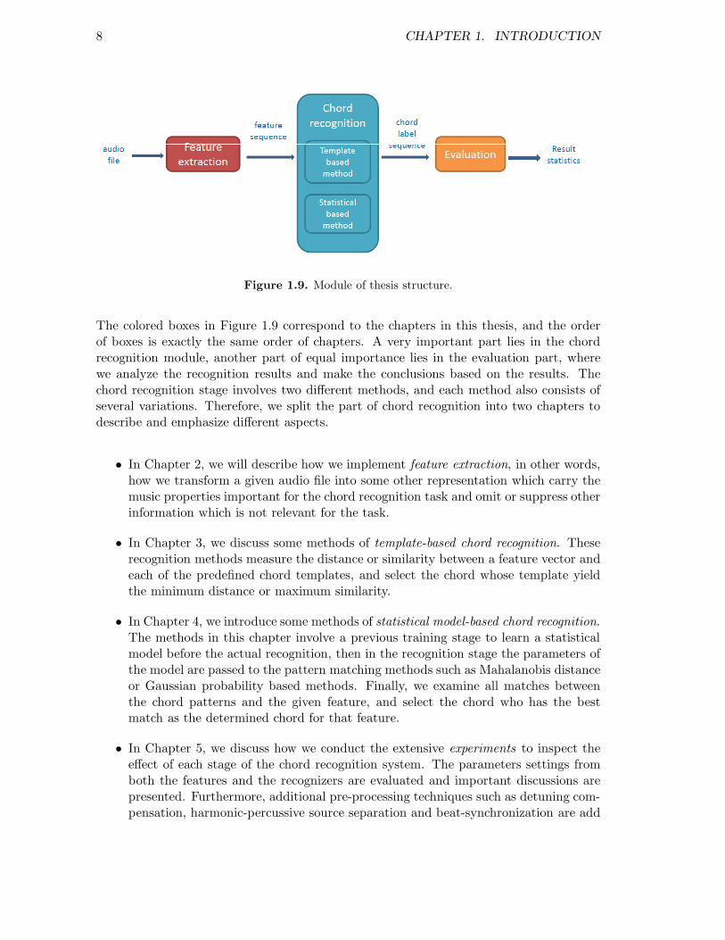
Since the algorithm of our chord recognition procedure is designed in a modular fash-ion, the structure of this thesis is also arranged corresponding to system implementation.Figure 1.9 shows the flowchart. Our system starts from the very left with audio file asan input, following the successive steps of feature extraction, chord recognition and eval-uation. Finally, we obtain some statistical results which reflect the performance of thesystem.
8 CHAPTER 1. INTRODUCTION
Figure 1.9. Module of thesis structure.
The colored boxes in Figure 1.9 correspond to the chapters in this thesis, and the orderof boxes is exactly the same order of chapters. A very important part lies in the chordrecognition module, another part of equal importance lies in the evaluation part, wherewe analyze the recognition results and make the conclusions based on the results. Thechord recognition stage involves two different methods, and each method also consists ofseveral variations. Therefore, we split the part of chord recognition into two chapters todescribe and emphasize different aspects.
• In Chapter 2, we will describe how we implement feature extraction, in other words,how we transform a given audio file into some other representation which carry themusic properties important for the chord recognition task and omit or suppress otherinformation which is not relevant for the task.
• In Chapter 3, we discuss some methods of template-based chord recognition. Theserecognition methods measure the distance or similarity between a feature vector andeach of the predefined chord templates, and select the chord whose template yieldthe minimum distance or maximum similarity.
• In Chapter 4, we introduce some methods of statistical model-based chord recognition.The methods in this chapter involve a previous training stage to learn a statisticalmodel before the actual recognition, then in the recognition stage the parameters ofthe model are passed to the pattern matching methods such as Mahalanobis distanceor Gaussian probability based methods. Finally, we examine all matches betweenthe chord patterns and the given feature, and select the chord who has the bestmatch as the determined chord for that feature.
• In Chapter 5, we discuss how we conduct the extensive experiments to inspect theeffect of each stage of the chord recognition system. The parameters settings fromboth the features and the recognizers are evaluated and important discussions arepresented. Furthermore, additional pre-processing techniques such as detuning com-pensation, harmonic-percussive source separation and beat-synchronization are add
1.6. ORGANIZATION OF THESIS 9
to our chord recognition system, we briefly examine their influence by comparingthe results with and without such techniques..
• At last in Chapter 6, we make conclusions about the whole thesis and discuss aboutfuture work.

10 CHAPTER 1. INTRODUCTION

Chapter 2
Feature Extraction
An audio file contains full of music information which consists of played notes, melody,harmony, beat, tempo, timbre of different instruments, dynamics of the sound, etc. Fora specific music processing task, only some of them is relevant and useful. Therefore weneed to select the most important information related to the specific task. Usually wename this processing stage as feature extraction, being the procedure of transforming anaudio file into a musically meaningful representation which keeps the most task-relatedmusical properties while suppressing other unrelated information. At the same time, theform of the representation should be appropriate for the next processing stage.
As the aimed music processing task discussed in this thesis is the chord recognition task,we need to extract audio features which emphasize the musical properties that refer tothe aspect of harmony. Such musical properties can be the chord progression, the melodyand component notes of a chord and their harmonics. Furthermore, a good feature shouldnot only be able to capture the music properties mentioned above but also suppress or beinvariant to some unrelated properties such as timbre and tempo.
As the chord itself is fully determined by its component notes, theoretically if the notes areknown, the chord could be identified. Thus the capture of notes plays a crucial role in thefeature extraction stage. Moreover, it is better to use pitch class 1 instead of single noteto describe the form of the chord since human beings’ perception of chords is irrelevantto the octave information of a note. Therefore our designed features should be able toproject the information for notes within the same pitch class and distinguish the notes indifferent pitch classes.
The reason that the features which used in chord recognition being invariant for timbreand tempo is obvious. For example, if two interpretations of a music piece are played bydifferent instruments which yield different timbre, the underlying notes are still the sameand therefore the chords formed by these notes are the same as well; if two interpretationsare interpreted with different speed, the underlying notes are still the same just their
1A pitch class is introduced due to the fact that human’s perception for pitch is periodic. Accordingto [23], a pitch can be separated into two components. One is referred to the tone height describing theoctave information, the other is the chroma or pitch class. The pitches in the same pitch class sound tohave similar ”quality” or ”color”. For example, the pitch class C is a set contains note C0,C1,C2, and soon.
11

12 CHAPTER 2. FEATURE EXTRACTION
duration change, which means the chords remain the same.
In the following sections, we introduce several features with all of them fulfilling therequirements mentioned above. In Section 2.1, we present pitch features which serve asbasis of the other features we use in our experiments. We describe how an audio file isdecomposed into spectral bands and then transformed into pitch features with the energyof each band within a short time summing up together. Then based on pitch features,we derive the following features which are in chroma2 representation in the subsequentsections. First, in Section 2.2, we talk about the common chroma features which summingup the spectral coefficients of the corresponding pitch features in the same chroma class.In Section 2.3 we modify the chroma features by performing logarithm compression onthe spectral coefficients before summing up. Then, in Section 2.4, adding a further degreeof abstraction by considering short-time statistics over energy distributions within thechroma bands, we obtain CENS (Chroma Energy Normalized Statistics) features, whichconstitute a family of scalable and robust audio features. To boost the degree of timbreinvariance, a novel family of chroma-based CRP audio features has been introduced [25,24]. We briefly describe CRP features in Section 2.5. Finally, CISP features from DanEllis’s group will be presented in Section 2.6.
Note that except CISP features, the implementations of MATLAB functions of all otherfeatures, respectively the Pitch, CP, CLP, CENS, CRP we mentioned in this thesis can befound in the Chroma Toolbox, which can be obtained in [22].
2.1 Pitch Features
2.1.1 Pitch Decomposition
In a first step, we decompose a given audio signal into 88 frequency bands correspondingto 88 musical notes from A0 to C8 which are of equal-tempered scale. Here we introducesome properties of a musical note. Firstly, a musical note can be identified by its MIDIpitch3 p, e.g., the note A4 corresponds to p = 69. Secondly, each note is associated with acertain frequency range with fixed center frequency, e.g., the note A4 has center frequency440 Hz. Furthermore, for each of the notes, its MIDI pitch number is related to its centerfrequency in some logarithm fashion:
Let p denote the pitch number, p ∈ [1 : 120], and let fp denote the center frequency of thepitch, then we have the relation:
fp = 2p−69
12 · 440 (2.1)
If we plug in pitch number p = 57 which is note A3, we will get the center frequencyf57 = 220 Hz, which is half of the center frequency of note A4. From this we can seethat if the pitch of a note is one octave higher than the other note, its center frequencywill be twice as the lower note’s. Besides, Equation (2.1) also implies that the higher the
2chroma has the same meaning as pitch class.3“The property of a sound that correlates to the perceived frequency is commonly referred to as the
pitch.” [23]

2.1. PITCH FEATURES 13
pitch is, the larger the frequency range it occupies. In our case, the decomposition fromthe audio signal to pitch subbands is realized by a multirate filter bank which consistsof an array of suitable bandpass filters. As the pitch gets higher, the bandwidth of thecorresponding filter gets wider. Figure 2.1 shows an illustration of the filter bank withdifferent bandwiths.
The decomposition from the original signal to 88 pitch related frequency subbands servesas a prerequisite signal processing step. It provides meaningful information about thesignal both in the temporal and the frequency domain, indicating at what time whichfrequency component is present. However, the great contribution of this step only works ifa pre-condition is fulfilled: we assumed that the audio file needs to have correct tuning andthe instruments are tuned according to the equal-tempered scale. In this way, tuning is acrucial factor which the multirate filter bank is sensitive to. In this thesis, we previouslytuned all the audio files before conducting any experiments in order to make sure thepitch features are correct. Besides this, strong onsets or string vibratos will lead to energyspreading in a large frequency range, affecting many subbands and therefore making thedecomposition problematic. Without prior detection and smoothing of these frequencyfluctuations, one may have imperfect subbands signals when such phenomena occur.
0 0.1 0.2 0.3 0.4 0.5−60
−40
−20
0
Figure 2.1. A sample array of filters with their respective magnitude responses in dB. (reproducedfrom [23])
2.1.2 Local Energy (STMSP)
The previous decomposition step allows us to identify the contribution which a certainpitch makes to the overall signal. However, the unit of measurement for the contribution ofeach pitch is not clear so far [33]. Also, the temporal measurement about the appearanceof note is also unclear. To solve this problem, we compute the short-time mean-squarepower (i. e., the samples of each subband output are squared) using a rectangular windowof a fixed length w. Denote a specific subband signal corresponding to pitch p as xp, kas the index of the sample points inside the window, n as the starting position of thewindow on the signal, then the STMSP is defined as
∑
k∈[n:n+w] |xp(k)|2. The window is
consistently shifted on the signal until the end with each time shifting it by a hop sizeh = w
2 , yielding 50% overlap between any of the two neighbor windows. The size of thewindow is usually chosen as a few milliseconds. Since the window size is closely related tothe hop size, and since the hop size is related with how frequent we get a feature from thesignal, or in other words, how large the feature rate is, we can directly deduct the featurerate as 1
h · 1000 which in our case being 2w · 1000(the multiplier 1000 is because that the
unit of hop size and window size is in millisecond, not second). For example, a windowlength corresponding to 200 milliseconds leads to a feature rate of 10 Hz.

14 CHAPTER 2. FEATURE EXTRACTION
The result after this processing step is a sequence of features which are referred to aspitch features. The pitch features measure the local energy content of each pitch subbandand indicate the presence of certain musical notes within the audio signal by selecting theenergy which exceed a certain threshold. See [23] for further details. The implementationof pitch features can be found in the MATLAB function audio_to_pitchSTMSP_via_FB.m
from the Chroma Toolbox[22].
As an example, we extracted pitch features from a synthesized audio file chordExample1.The audio file consists of five chords, its score representation is shown in Figure 2.2(a).Figure 2.2(b) shows the spectrogram of the original signal with x-axis indicating the timein seconds and y-axis indicating the frequency in a linear way, with the unit Hertz. Fig-ure 2.2(c) shows the extracted pitch features with y-axis indicating the MIDI pitch number,which associated with frequency in a logarithmic way. The colored intensity representsthe STMSP value or local energy. Here, the played notes can be clearly identified in thelower part of Figure 2.2(c). However, as we can observe from the upper part, there arecomparably low intensities for some unplayed notes, which are actually caused by theharmonics of the played notes. This phenomenon implies a common challenge in chordrecognition task: even with the synthesized example which consists of only one instrument,the presence of harmonics will affect the identification of played notes. In our example,the intensities of harmonics are weak, however in real audio files which involve severalinstruments, the harmonics caused by different instruments will be blend together withthe real played notes. Sometimes the intensities of harmonics are as large as some softplayed notes, which make the identification of real played notes more difficult.
2.2 Chroma Features
As we discussed in the last section, the energy caused by a certain played note is not onlypresent at the exact frequency that note covers but also at higher frequencies where theharmonics of the note are located. This makes not only the identification of a musical notedifficult, but also the identification of component notes of a certain chord difficult. In thissection, we introduce a new type of feature named as chroma features which can partlysolve this problem. Chroma-based audio features are a well-established tool in processingand analyzing music data [2, 9, 23], and the chroma features are particularly suitable forchord recognition.
As we know that human’s perception of musical notes has a certain character: if a noteis one or more octave higher than another note, then the two notes sound to have thesame “tone color” but different “tone height”. This phenomenon is referred to as octaveequivalence in music theory. Assuming the musical notes are of equal-tempered scale,the chroma correspond to the set {C,C],D, . . . ,B} that consists of the twelve pitch spellsattributes as used in Western music notation. Note that in the equal-tempered scale,different pitch spellings such as C] and D[ refer to the same chroma.
Take MIDI notation for example, note A4 denotes the chroma as A and “tone height”as the 4th octave. We can reduce the MIDI notes from 88 pitches to 12 chroma classesby ignoring the octave information of the notes and classifying via chroma information.Chroma features are very suitable for the task of chord recognition. This is because when

2.2. CHROMA FEATURES 15
(a) score representation
time
freq
uenc
y(H
z)
0 1 2 3 4 5 6 7 8 9 100
500
1000
1500
2000
2500
3000
3500
4000
4500
5000
0
0.5
1
1.5
2
2.5
3
(b) spectrogram
time
mid
i pitc
h nu
mbe
r
0 1 2 3 4 5 6 7 8 9 1054
60
66
72
78
84
90
−30
−25
−20
−15
−10
−5
0
5
(c) pitch representation
Figure 2.2. Score representation, spectrogram and pitch representation of the synthesized musicaudio ChordExample1.
analyzing a musical chord, we are much more interested in the chroma (or pitch class)which the note belongs to other than the absolute pitch of that note. For notes sharingthe same chroma but in different octaves, we treat them as identical when considering acomponent note of the chord. Furthermore, remember that different timbre of instrumentswill yield different yet distinctive energy distribution at harmonics, and since the energyof a chroma is merged from different pitches corresponding to this chroma together, thedifference caused by timbre is well absorbed by chroma features, thus making them robustto the variations of timbre.
The chroma features are in the form of a 12-dimensional vector x = (x(1), x(2), . . . , x(12))T ,where x(1) corresponds to chroma C, x(2) to chroma C], and so on. Chroma-based fea-tures represent the short-time energy of the signal in each of the 12 pitch classes. Oftenthese chroma features are computed by suitably pooling spectral coefficients obtained froma short-time Fourier transform [2, 9]. Similarly, one can start with the pitch representa-tion introduced in Section 2.1. Then, by simply adding up the corresponding values thatbelong to the same chroma, one obtains a chroma representation or chromagram. Usuallywe perform `2 normalization on the resulting vectors. For the case of near silence or weaknoise, the sum of all entries of such chroma vector will be quite small. If the sum fallsbelow a certain threshold, we replace the original chroma vector by the unit vector.

16 CHAPTER 2. FEATURE EXTRACTION
In the following, the resulting features are referred to as Chroma-Pitch and we denotethem by CP, see [23] for more details. The MATLAB function of this part can be foundin pitchSTMSP_to_chroma.m from our toolbox.
Figure 2.3 illustrates the chromagram of feature CP extracted from the audio file ChordEx-ample1. The figure in the middle shows the features in the middle step which is after spec-tral pooling, the figure at bottom shows the final chroma features generated by spectralpooling with `2 normalization. In Figure 2.3(b), only the onset can be clearly seen in thefirst 0.5 second of each chord, the intensity of the remaining duration is not visible. In thiscase we cannot distinguish between the real silence and the remaining sound. However inFigure 2.3(c), the silence can be clearly identified through the unit vector whose energy iseverywhere the same for all chromas. Besides, not only the onset but also the remainingduration can be easily seen, especially for the bass note of each chord (red color in thefigure).
Note that CP features still imperfect. For example, from 5.8 to 7.5 seconds in Figure 2.3(c),the chroma G is much stronger than the other two component notes. As the bass noteand also the root note of the G, its comparably large intensity makes sense. But it shouldnot be so strong that the intensity of other notes are nearly erased after normalization,which make the identification of the other two notes problematic. This is also the case forthe chroma F from 5.8 to 7.5 seconds. This imperfection requires further processing stepto further balance the difference of intensity.
(a) score representation
0 1 2 3 4 5 6 7 8 9 10
C
C#
D
D#
E
F
F#
G
G#
A
A#
B
−30
−25
−20
−15
−10
−5
0
5
(b) chroma features without normalization
0 1 2 3 4 5 6 7 8 9 10
C
C#
D
D#
E
F
F#
G
G#
A
A#
B
0
0.1
0.2
0.3
0.4
0.5
0.6
0.7
0.8
0.9
1
(c) chroma features with normalization
Figure 2.3. Score representation and chromagram of CP extracted from ChordExample1.

2.3. CHROMA FEATURES WITH LOGARITHMIC COMPRESSION 17
2.3 Chroma Features with Logarithmic Compression
To account for the logarithmic sensation of sound intensity [18, 36], one often applies alogarithmic compression when computing audio features [15]. Besides, this step also worksas adjusting the dynamic range of the original signal to enhance the clarity of weakertransients, especially in the high-frequency regions [11]. There are some weak chromaswhose intensities are very low. Such chromas are difficult to identify in the chromagramof CP. With the help of logarithmic compression, now it is easy to find their existence.
The procedure of how we derived the chroma features with logarithmic compression ispresented as follows. Firstly, we compute pitch features from the audio file as we describedin Section 2.1. Secondly, the pitch representation is logarithmized by replacing each entrye by the value log(η · e + 1), where η is a suitable positive constant. Thirdly, we convertthe logarithmic pitch features into the chroma representation by spectral pooling and `2
normalization as we described in Section 2.2. The resulting features are named as ChromaFeatures with Logarithmic Compression and denoted as CLP(η) where the parameter ηspecifies the extent of logarithmic compression. The role of η, which is set to η = 1000 inmost of our experiments, is evaluated in Section 5.3.3.
0 1 2 3 4 5 6 7 8 9 10
C
C#
D
D#
E
F
F#
G
G#
A
A#
B
0
0.1
0.2
0.3
0.4
0.5
0.6
0.7
0.8
0.9
1
(a) CLP(1)
0 1 2 3 4 5 6 7 8 9 10
C
C#
D
D#
E
F
F#
G
G#
A
A#
B
0
0.1
0.2
0.3
0.4
0.5
0.6
0.7
0.8
0.9
1
(b) CLP(10)
0 1 2 3 4 5 6 7 8 9 10
C
C#
D
D#
E
F
F#
G
G#
A
A#
B
0
0.1
0.2
0.3
0.4
0.5
0.6
0.7
0.8
0.9
1
(c) CLP(100)
0 1 2 3 4 5 6 7 8 9 10
C
C#
D
D#
E
F
F#
G
G#
A
A#
B
0
0.1
0.2
0.3
0.4
0.5
0.6
0.7
0.8
0.9
1
(d) CLP(1000)
Figure 2.4. CLP features extracted from ChordExample1.
As an illustrative example, Figure 2.4 provides the chromagrams of CLP(η) with η =1, 10, 100, 1000 respectively. As we can see from the figure, as η gets larger, the intensitycontrast between different chroma gets smaller. For example, for the period from 9.0to 9.5 seconds, in Figure 2.4(a) the chroma C and A are almost invisible. However inFigure 2.4(d) they can be clearly seen. In particular, the chroma C is more obvious. Thishelps us to identify the underlying chord F for that period, because all three componentnotes of F are present. This is much better than the situation where the intensity of onlyone chroma can be observed while the intensity for other chromas are too low to find. Inthis situation, it is too hard to decide the underlying chord.
One can observe in Figure 2.4 that the original pause period such as 1.5 to 1.9 seconds
18 CHAPTER 2. FEATURE EXTRACTION
is disappearing as η is increasing. This is a typical evidence that weak intensity will beenhanced by logarithmic compression. In contrast, the chroma C from 0.5 to 1.2 secondschanging the color from red to yellow, which means that the intensity gets less and lessas η increases. This is evidence that the original strong intensity will be suppressed toa milder degree. In this way, the logarithmic compression is balancing the difference ofintensity, and the η is the controlling parameter of such balance.
2.4 CENS Features
Generally speaking, the Chroma-Pitch features have already achieved the goals of featuredesign aimed for chord recognition since it is able to indicate the behavior of harmonic pro-gression of a music piece. However, it can still be further improved considering variationsof musical properties such as dynamics, timbre, articulation, execution of note groups,and temporal micro-deviations. In order to be robust against these variations, we add afurther degree of abstraction to Chroma-Pitch features by considering short-time statisticsover energy distributions within the chroma bands. The features we obtained are namedas CENS (Chroma Energy Normalized Statistics) features, and they constitute a familyof scalable and robust audio features. CENS features, which have first been introducedin [26], are strongly correlated to the short-time harmonic content of the underlying audiosignal while absorbing variations in other parameters. Furthermore, because of their lowtemporal resolution, CENS features can be processed efficiently, see [26, 23] for details.
In computing CENS features, we have five stages with each designed for a different purpose.The computing pipeline is shown in the following:
1. Normalization. First, we `1-normalize the chroma features in order to absorb differ-ences in the sound intensity or dynamics. For the case of very low energy distributionor silence, we replace the chroma vector by a uniformly distributed vector if the normdoes not exceed certain threshold.
2. Quantization. The component of the normalized chroma vector are quantized basedon logarithmically chosen thresholds to simulate the humans’s perception of loudness.This introduces some kind of logarithmic compression similar to the features CLP.The quantization function serves as a mapping function from [0, 1] to {0, 1, 2, 3, 4}.
3. Smoothing. The quantized vectors from last step are now convolved with a Hannwindow of fixed length w, w ∈ N. This step works as temporal smoothing to blendin the context information and reduce the influence of local error.
4. Downsampling. We downsample the resulting feature vectors by a specific factor dto increase the computation efficiency for the next processing module.
5. Normalization. Finally, we perform `2-normalization to the feature vectors.
In the following, we denote the resulting CENS features by CENS(w, d) with w indicatingthe size of convolution window and d indicating the downsampling factor. The MAT-LAB function of this part can be found in pitchSTMSP_to_CENS.m from the ChromaToolbox [22].

2.4. CENS FEATURES 19
0 1 2 3 4 5 6 7 8 9 10
C
C#
D
D#
E
F
F#
G
G#
A
A#
B
0
0.1
0.2
0.3
0.4
0.5
0.6
0.7
0.8
0.9
1
(a) CENS(1, 1)
0 1 2 3 4 5 6 7 8 9 10
C
C#
D
D#
E
F
F#
G
G#
A
A#
B
0
0.1
0.2
0.3
0.4
0.5
0.6
0.7
0.8
0.9
1
(b) CENS(21, 1)
0 1 2 3 4 5 6 7 8 9 10
C
C#
D
D#
E
F
F#
G
G#
A
A#
B
0
0.1
0.2
0.3
0.4
0.5
0.6
0.7
0.8
0.9
1
(c) CENS(41, 1)
Figure 2.5. CENS features extracted from ChordExample1.
The main purpose of using CENS features in our chord recognition system is to take advan-tage of its internal effect of smoothing at the feature side. This serves as the pre-filteringbefore the chord recognition module. We also provide chord recognition methods perform-ing smoothing on the recognizer side, which serves as the post-filtering of the final chorddecisions. Figure 2.5 illustrate chromagrams with different smoothing window length ofCENS features. Having a feature rate of 50 Hz, each feature vector contains music informa-tion of 0.02 seconds for the non-smoothing version, which is CENS(1, 1), since w = 1 meansconvolve with the current feature itself. By enlarging w to 21, each feature vector nowcarries the music information of 0.02 · 21 = 0.42 second. By comparing Figure 2.5(b) andFigure 2.5(a) we find that the unit vectors corresponding to silence period are smoothedout by the neighbor C. This means that chords tend to be continuous via smoothing.Furthermore by enlarging w to 41, we find that the edge of the chord gets more blurred.For example, at around 7.5 second, the chroma G and D should stop. In CENS(1, 1) it issilence for all chromas at that time point which helps us to make exact decision about theedge of G. However in CENS(41, 1) at that time point, due to the large smoothing window,the presence of G and D coming from the left neighbor features, and A, F, C coming fromthe right neighbor features mix together. This might leads to errors in chord recognition,and it is hard to decide the edge in the situation when a previous chord finishes or when
20 CHAPTER 2. FEATURE EXTRACTION
a new chord starts.
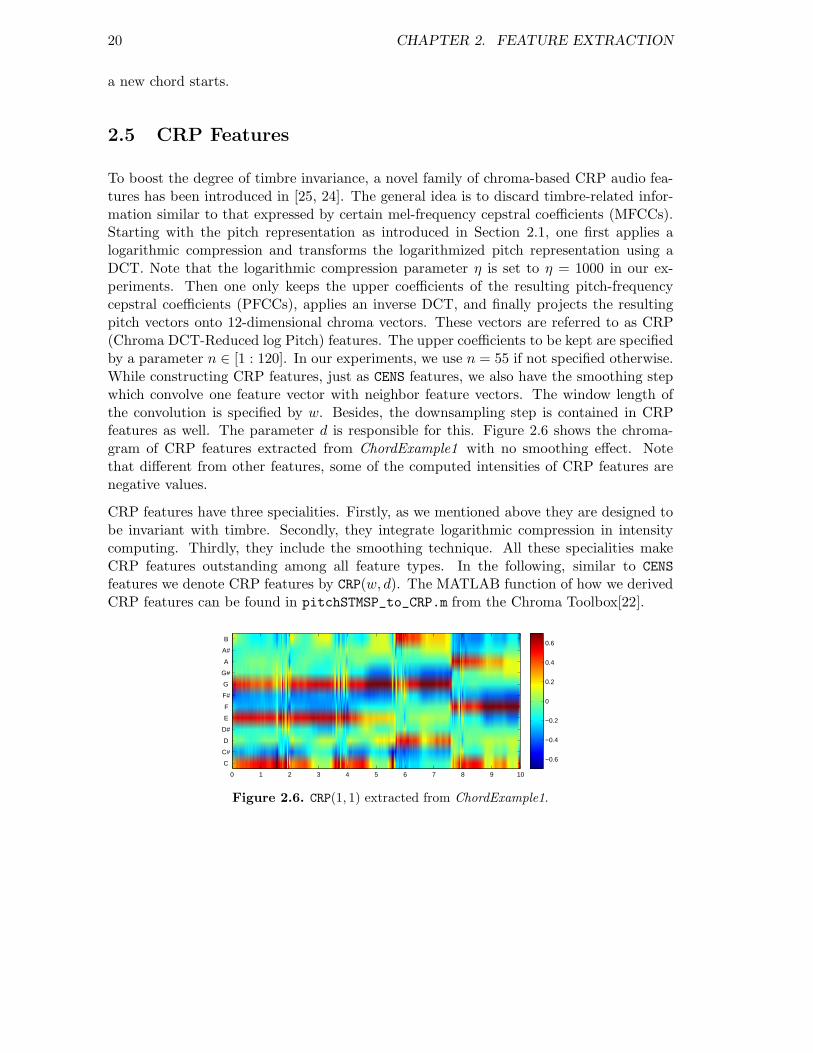
2.5 CRP Features
To boost the degree of timbre invariance, a novel family of chroma-based CRP audio fea-tures has been introduced in [25, 24]. The general idea is to discard timbre-related infor-mation similar to that expressed by certain mel-frequency cepstral coefficients (MFCCs).Starting with the pitch representation as introduced in Section 2.1, one first applies alogarithmic compression and transforms the logarithmized pitch representation using aDCT. Note that the logarithmic compression parameter η is set to η = 1000 in our ex-periments. Then one only keeps the upper coefficients of the resulting pitch-frequencycepstral coefficients (PFCCs), applies an inverse DCT, and finally projects the resultingpitch vectors onto 12-dimensional chroma vectors. These vectors are referred to as CRP(Chroma DCT-Reduced log Pitch) features. The upper coefficients to be kept are specifiedby a parameter n ∈ [1 : 120]. In our experiments, we use n = 55 if not specified otherwise.While constructing CRP features, just as CENS features, we also have the smoothing stepwhich convolve one feature vector with neighbor feature vectors. The window length ofthe convolution is specified by w. Besides, the downsampling step is contained in CRPfeatures as well. The parameter d is responsible for this. Figure 2.6 shows the chroma-gram of CRP features extracted from ChordExample1 with no smoothing effect. Notethat different from other features, some of the computed intensities of CRP features arenegative values.
CRP features have three specialities. Firstly, as we mentioned above they are designed tobe invariant with timbre. Secondly, they integrate logarithmic compression in intensitycomputing. Thirdly, they include the smoothing technique. All these specialities makeCRP features outstanding among all feature types. In the following, similar to CENS
features we denote CRP features by CRP(w, d). The MATLAB function of how we derivedCRP features can be found in pitchSTMSP_to_CRP.m from the Chroma Toolbox[22].
0 1 2 3 4 5 6 7 8 9 10
C
C#
D
D#
E
F
F#
G
G#
A
A#
B
−0.6
−0.4
−0.2
0
0.2
0.4
0.6
Figure 2.6. CRP(1, 1) extracted from ChordExample1.

2.6. CISP FEATURES 21
2.6 CISP Features
In this section, we adapt the chroma feature extraction according to Dan Ellis’ s instan-taneous frequency-based chromagram and we name this feature as CISP features. UsingCISP features, we can identify strong tonal components in the spectrum and to get ahigher-resolution estimate of the underlying frequency [7]. While generating chroma rep-resentation features, using a coarse mapping of FFT bins to the chroma classes whichthe bins overlap will often yield blurry low frequencies. CISP take advantage of phase-derivative (instantaneous frequency) within each FFT bin, and get a finely estimation offrequency.
A further motivation of using instantaneous frequency lies in that sinusoidal componentsof the audio signal contains the most relevant information about the melody [6], whichis the tonal component of music. CISP is intended to remove nontonal components andimprove frequency resolution beyond FFT bin level [7].
CISP features are constructed as follows. Firstly, a spectrogram is computed using a shorttime fourier transform. Secondly, for each of the bins of the spectrogram (every bin boundsa range of frequencies), the instantaneous frequency is determined. Thirdly, based on theinstantaneous frequency, a noise harmonic component separation is performed. Note thatthe frequency of a bin is estimated by weighted sum of the frequencies inside the bin withthe weights being the corresponding magnitude of those frequencies. Finally, the estimatedfrequencies are mapped into chroma representation by adding up the magnitude of binswhich belong to the same chroma.
CISP feature integrates an automatic tuning step. To avoid problems of tuning, themapping of frequencies to chroma bins is adjusted by up to ±0.5 semitones to make thesingle strongest frequency peak line up exactly with a chroma bin center [7].
Figure 2.7(a) indicates the color-coded instantaneous frequency values for each bin of aspectrogram. The x-axis indicates the frame number and y-axis indicates the the numberof bins. See Figure 2.7(b) for the corresponding magnitude spectrogram. Here, a frequencyof zero value (the dark blue in Figure 2.7(a)) indicates that this bin was selected as noiseand filtered out. One can observe from the remaining horizontal structures, which areactually the harmonic components. Figure 2.7(c) illustrates the chroma representation ofCISP features. We can observe that CISP features are very sensitive to small magnitudes.The computed intensity at B and D are much larger than other features. However, Band D are only harmonics which have much smaller magnitudes compared to the othercomponent notes of C. In the other chromagrams which we presented previously, they canhardly be seen.
The MATLAB Function of CISP features can be found in the Intelligent Sound ProcessingToolbox [5]. In the following passages, we denote CISP features as CISP.

22 CHAPTER 2. FEATURE EXTRACTION
50 100 150 200 250 300 350 400
20
40
60
80
100
120
140
200
400
600
800
1000
1200
1400
(a) Tracked instantaneous frequency
50 100 150 200 250 300 350 400
20
40
60
80
100
120
140
0
0.05
0.1
0.15
0.2
0.25
0.3
(b) Spectrum of STFT
0 1 2 3 4 5 6 7 8 9
C
C#
D
D#
E
F
F#
G
G#
A
A#
B
0
0.1
0.2
0.3
0.4
0.5
0.6
0.7
0.8
0.9
1
(c) Chroma representation
Figure 2.7. Tracked frequencies, tracked magnitude, and chroma representation of CISP featuresextracted from ChordExample1.

Chapter 3
Template-based ChordRecognition
After converting the audio file into musically meaningful audio features, we now pass thesefeatures into the chord recognition module which automatically classify the feature vectorswith respect to given chord labels. In other words, the chord recognition module assignsto each feature vector a chord label.
From this chapter on, we begin to discuss chord recognition methods. In this chapter wefocus on template-based methods. In these methods, firstly, some pre-computed featuretemplates are defined and they served as chord patterns. Here, the templates can bedefined from different point of views and therefore have many variations. Secondly, weneed to compare how similar a given feature vector is to each of the templates. To thisend, we need to find a similarity measure or distance measure between the feature anda template. Thirdly, we assign the chord label by selecting the one which yields themaximum similarity or minimum distance to the given feature.
The remainder of this chapter is organized as follows. We start by introducing the generalprocedure of template-based recognition methods in Section 3.1. Then three differentspecifications of template sets, namely the binary templates, the harmonically enrichedtemplates and the averaged templates, will be described in Section 3.2. After that wepresent the setting of distance measure. In particular, the specification of cosine distanceis introduced in Section 3.3. Finally, in Section 3.4, we summarize the advantages anddisadvantages of using template-based methods.
3.1 Template-based Chord Recognition
In the previous stage of feature extraction, we transform a given audio recording intoa chroma-based feature sequence X := (x1, x2, . . . , xN ), xn ∈ F := R
12, n ∈ [1 : N ].Here in the stage of chord recognition, we use template-based recognizers to assign chordlabels to the feature sequence. In this section, we will describe the general procedure oftemplate-based chord recognition. The procedure can be described as follows.
23

24 CHAPTER 3. TEMPLATE-BASED CHORD RECOGNITION
• Firstly, we define our set of templates. Given a chord label set Λ, the template setT is a subset of the feature set F . T consists of 24 chroma-based chord patternscorresponding to 12 major and 12 minor triads. The elements of T are indexed bythe element of chord label set Λ. we denote a template as tλ ∈ T ,(λ ∈ Λ).
• Secondly, in order to compute the distance between a feature vector and a chordtemplate, we need a distance measure. Since a template is a feature vector withspecial meaning, we fix the distance measure d : F×F → R. This distance measureshow different a feature vector compared to a chord template.
• Finally, for a given feature vector, we compute its distance with each of the chordtemplates. Now the template-based chord recognition procedures simply consistsin assigning the chord label that minimizes the distance between the correspondingtemplate and the given feature vector x = xn:
λx := argminλ∈Λ
d(tλ, x). (3.1)
Both the template set and the distance measure are not fixed in the procedure. In thefollowing passages, we complete the procedure with three template settings defined fromdifferent aspects of chords and use cosine distance as measurement. By changing thetemplates or distance, one can check the different recognition results and further inspectwhether a certain template setting is meaningful and whether it is suitable for the giventype of features. Besides, the template-based methods work in a purely framewise fashionand no temporal context is considered. We are not the first one to use template-basedmethods as chord recognizers, similar previous work can be found in [12, 17, 28].
3.2 Specification of Chord Template Sets
In this section, we consider three variations of template setting. Remember that thetemplate set T is a subset of the feature set F = R
12, that is to say, a template is also afeature vector. However, a template has a special meaning compared to the normal featurevectors which extracted from audio files, because it describes a certain chord pattern inthe representation of a feature vector. It can be set variously from different point of views.The three variations of template setting which we introduce in this section only differ inhow the weights are setted to the entries of the template vector. The weights can eitherbe manually set considering the theoretical characteristic of a chord, or they can be setby learning their general characteristics from the real data in practice.
Here are the three variation of templates:
• Set of binary templates: T b with elements tbλ
• Set of harmonically enriched templates: T h with elements thλ
• Set of average templates: T a with elements taλ

3.2. SPECIFICATION OF CHORD TEMPLATE SETS 25
The details of how we set the templates will be described in the following subsections.There is an a general trick which is named as “cyclically shift”, and it is used in all thetemplate setting. We first introduce it here.
3.2.1 Cyclically Shift
For each of the template sets, we only set two templates instead of setting all templates.We set one for C and the other for Cm, and denote them as tC and tCm. The templatesfor other major triads are computed by cyclically shifting tC, and other minor triads arecomputed by cyclically shifting tCm. The reason of involving cyclically shift is to utilize thecharacteristics of the chords. Since the musical interval between the third and root, fifthand root are always fixed for the same type of chord, one can derive the same type of thechords by first changing the root note and then make sure the third and fifth note fromthe musical interval. Therefore, we can derive the templates for the same type of chordsby cyclically shifting the position of the notes.
Thus for later usage, we define an operation that allows for cyclically shifting the compo-nents of a feature vector x := (x(1), . . . , x(D))T ∈ F . To this end, we introduce the shiftoperator σ : F → F defined by
σ((x(1), . . . , x(D))T) := (x(D), x(1) . . . , x(D − 1))T. (3.2)
Iteratively applying the shift operator, one obtains
σi(x) = σ(σi−1(x)). (3.3)
for i ∈ Z. Obviously, σD = σ0 is the identity on F . Therefore, in the following, we onlyconsider the shift index i moduloD. We extend the shift operator to the space of sequencesFN in a canonical way and denote the resulting operator again by σ : FN → FN :
σ(X) := (σ(x1), σ(x2), . . . , σ(xN )), (3.4)
for a given sequence X := (x1, x2, . . . , xN ) ∈ FN .
3.2.2 Binary Templates
The first template setting introduced here is designed to be the simplest one among allthe settings. The motivation of introducing binary templates is to simulate the fact thata chord is formed by its component notes1. For example, C is composed by the note C, Eand G; Cm is composed by C, E[ and G. While designing the templates in this method,for every given chord, we only consider the component notes of chord and totally discardother non-component notes. Thus it is reasonable to involve a binary setting since a noteis either a component or a non-component one.
We set the binary templates as follows. Each template in the set T b is a 12-dimensionalbinary vectors with three entries equal to one and other entries equal to zero. The threenon-zero entries correspond to the three component notes of a chord.
1Here the notes we mentioned are as chromas, which come from distinctive pitch classes

26 CHAPTER 3. TEMPLATE-BASED CHORD RECOGNITION
C C# D D# E F F# G G# A A# B 0
0.1
0.2
0.3
0.4
0.5
0.6
0.7
0.8
0.9
1
(a) tbC
C C# D D# E F F# G G# A A# B 0
0.1
0.2
0.3
0.4
0.5
0.6
0.7
0.8
0.9
1
(b) tbCm
Figure 3.1. Binary templates for C and Cm.
For example, the binary template corresponding to C C = {C,E,G} is given by
tbC = (1, 0, 0, 0, 1, 0, 0, 1, 0, 0, 0, 0)T .
The binary template corresponding to Cm Cm = {C,E[,G} is given by
tbCm = (1, 0, 0, 1, 0, 0, 0, 1, 0, 0, 0, 0)T .
Figure 3.1 illustrates the setting of binary templates for C and Cm. We denote a binarytemplate by tb. Note that we perform the `2-normalization on the values shown above inorder to fit the features which are also with `2-normalization. The advantage of the binarysetting is its simplicity and efficiency. The same weights on the component notes is fairto count the contribution from each of the component notes. In contrast, the simplicityalso leads to a limitation: it considers only the very ideal instance of a chord which workstheoretically. However in practice, the intensity of the three component notes may not beexactly the same but very different. Also, it ignores too much information, for instance,it totally disregard the non-component notes, which may contribute to form the patternof a chord.
3.2.3 Harmonically Enriched Templates
For the recognition method using harmonically enriched templates, the weights for theentries of a template considers not only the component notes of a chord but also theirharmonics. The motivation of this method is to simulate a phenomenon in practice thatwhen a single note is played on instrument, the sound is not a simple pure tone with a well-defined frequency [23]. According to [23], “the sound of a musical tone can be regarded asa superposition of harmonics or overtones - whose frequencies differ by an integer multiplefrom a certain fundamental frequency.”. Here, the fundamental frequency is the frequencyof the lowest harmonics. If the fundamental frequency is f , the harmonics have frequencies2f , 3f , 4f , etc. For example, on piano, if one presses the key which has the MIDI pitchC4, one can only recognize the sound as C4 by human’s perception. However, actually thesound the piano generates contains not only C4, but also its harmonics. These harmonicsinclude C5 which has double times of frequency of C4, G5 which has triple times, C6 whichhas four times, and so on.
The reason why humans can not perceive the harmonics lies in the intensity or loudness ofthe harmonics. Take piano for instance, the intensity of the harmonics are much smaller

3.2. SPECIFICATION OF CHORD TEMPLATE SETS 27
than the intensity of the note which has the fundamental frequency. Especially, the higherthe harmonics, the smaller the intensity. The note at fundamental frequency contributesthe most to the overall intensity. This is the usual case for piano, but not universal forany of the instruments. For some instruments, it might be the case that the first harmoniccontributes the most of intensity and what humans perceive is the sound of 1st harmonic,while the sound of fundamental frequency can hardly be perceived.
In this thesis, we set up the simulation of harmonics in the way that Emilia Gomezsuggested in [10]. She modeled the harmonics of notes using simulating the spectralenvelope. To this end, we set the weights to the notes of a chord as follows. Firstly,we assign the theoretical amplitude to all component notes of a chord. Secondly, foreach of the component notes, we consider its harmonics. For each harmonic, we assign atheoretical amplitude, and this amplitude is related to which overtone the harmonic is forthe component note. The value is assigned by an empirical decay factor s multiplied bythe amplitude of component notes. The decay factor is to model the amplitude of differentharmonics such that the contribution decrease as the frequency increase [29]. Gomez sets as 0.6.
The contribution for the first 6 harmonics of a note is given in Table 3.1. In this way,for each component note of a chord, its intensity contribution to the chord consists of theintensity from the component note itself, and the intensity from all its harmonics. Sincethe 1st harmonic is just the component note itself, the added intensities are coming fromthe other 5 higher harmonics. We include all these values in our templates. In order toavoid zero weight for any of the notes, we initially set the weights of all notes to a verysmall value ε = 0.005 instead of zero.
Table 3.2 present the information about the frequency and index of the harmonics and thecorresponding decayed factor for the component note C4, E4 and G4 of chord C, assumingthe notes are played in the fourth octave. The resulting harmonic template considersall the contributions from the notes in these tables and project these contributions into12-dimensional chroma representation. The resulting template are as follows:
The harmonic template correspond to C C = {C,E,G} with decay factor s = 0.6 is givenby
thC = (0.254, 0.005, 0.061, 0.005, 0.272, 0.005, 0.005, 0.315, 0.018, 0.005, 0.005, 0.079)T .
The harmonic template correspond to Cm Cm = {C,E[,G} with decay factor s = 0.6 isgiven by
thCm = (0.254, 0.005, 0.612, 0.254, 0.018, 0.005, 0.005, 0.333, 0.005, 0.005, 0.061, 0.018)T .
Figure 3.2 illustrates the final harmonic templates for C and Cm. This is also the versionwith `2-normalization. We denote a harmonically enriched template by th.
3.2.4 Averaged Templates
In this setting, the template vector is not composed of manually set values anymore,but values derived from averaging of practical training data. This also means that the

28 CHAPTER 3. TEMPLATE-BASED CHORD RECOGNITION
index frequency factor1 f 12 2f s3 3f s2
4 4f s3
5 5f s4
6 6f s5
Table 3.1. Contributions for the first six harmonics of a note.
index note frequency factor1 C4 fC4 12 C5 2fC4 s3 G5 3fC4 s2
4 C6 4fC4 s3
5 E6 5fC4 s4
6 G6 6fC4 s5
index note frequency factor1 E4 fE4 12 E5 2fE4 s3 B5 3fE4 s2
4 E6 4fE4 s3
5 G]6 5fE4 s4
6 B6 6fE4 s5
index note frequency factor1 G4 fG4 12 G5 2fG4 s3 D6 3fG4 s2
4 G6 4fG4 s3
5 B6 5fG4 s4
6 D7 6fG4 s5
Table 3.2. Contributions for the first six harmonics of component notes of C. Assuming thechords is played in the 4th octave. From left to right corresponding to the notes C4, E4 and G4.
C C# D D# E F F# G G# A A# B 0
0.1
0.2
0.3
0.4
0.5
0.6
0.7
0.8
0.9
1
(a) thC
C C# D D# E F F# G G# A A# B 0
0.1
0.2
0.3
0.4
0.5
0.6
0.7
0.8
0.9
1
(b) thCm
Figure 3.2. Harmonically enriched templates for C and Cm.
templates we describe in this set are not fixed as the previous binary or harmonicallyenriched setting, but vary according to different training datasets. These are the mostsignificant differences compared to the previous two settings.
Figure 3.3 illustrates the procedure of generating the averaged templates. The typicaltraining data basically consists of some music audio files and corresponding chord annota-tion labels. We divide all the training data we have into several partitions, and call eachof the partition a training dataset. Since our system is evaluated in a framewise fashion,we need to divide the training data into the form of frames, meaning that we segmentthe audio files into feature frames and parse the annotation files into label frames. Theaudio files are transformed into the feature vectors in the stage of feature extraction, andthe chord annotation labels are parsed and aligned with the feature vectors in this stage.For example, if the feature rate is 10Hz, and we have an annotation of C from 1.1 to 2.0seconds, then there will be 10 feature vectors with each of them occupying 0.1 second ofthis period and labeled with C. The number of label frames is exactly corresponding tothe number of feature frames. In case the annotation file is not completely annotated, forthe intervals without annotation, we set it to “N” indicating non-annotation.
After that we have many feature vectors with the ground truth chord labels in hand.Usually we do not know whether we could cover all chords in the training data so that

3.2. SPECIFICATION OF CHORD TEMPLATE SETS 29
we have at least one instance for each of the chord. Even if we could cover all the chords,some chords might have too few instances. To avoid this problem, we shift all featureframes and their chord labels to C or Cm. To achieve this, we perform cyclically shifting onall non C-labeled or Cm-labeled features. After that, all feature vectors are cyclicly shiftedfrom different chords to C or Cm. This procedure works as follows.
1. First we need to compute how many semitones are needed to shift from an arbitrarychord with label λ1 to the objective chord with label λ2. To achieve this, we definethe following two functions.
Suppose we have a mapping function M : Λ → Z, which maps a chord to a positiveinteger i, i ∈ [1 : 24], starting from i = 1 indicating C, i = 2 indicating C], i = 13indicating Cm, i = 14 indicating C]m and so on. Table 3.3 shows the mapping fromall major and minor triads to corresponding numbers. Furthermore we define thefunction dchord : Λ × Λ → Z to compute the semitone distance between the twochords λ1 and λ2 :
dchord(λ1, λ2) := |M(λ1)−M(λ2)| . (3.5)
2. Denote the feature frame corresponding to the label λ1 as x1, which is the one tobe shifted. Also denote the result feature frame x2 corresponding to the label λ2,which is the objective feature we want. Then x2 is computed as :
x2 = σ(dchord(λ1,λ2))(x1). (3.6)
Note that we shift major chords to C and minor chords to Cm .
Figure 3.3. Procedure of generating the averaged template T a.

30 CHAPTER 3. TEMPLATE-BASED CHORD RECOGNITION
chord name mapped valueC 1C] 2D 3D] 4E 5F 6F] 7G 8G] 9A 10A] 11B 12
chord name mapped valueCm 13C]m 14Dm 15D]m 16Em 17Fm 18F]m 19Gm 20G]m 21Am 22A]m 23Bm 24
Table 3.3. Mapping function dchord for major and minor triads.
Here we take a feature vector xG = ((x(1), . . . , x(12)) for example, since we want tocyclically shift it to C, the semitone distance dchord(λC , λG) = |M(λG)−M(λC)| = 8−1 =7, thus xC = σ(dchord(λG,λC))(xG) = σ7(xG) = ((x(8), . . . , x(12), x(1), . . . , x(7)).
After the step cyclically shifting, all features vectors are either C or Cm. The huge amountof instances allows us to estimate the average value as template more convincible. Itshould be much better than estimating the average value for each chord while relying ona small amount of instances, which is not capable to reveal the real pattern of the chords.Now we consider the averaged feature vector of C as the template for C, and the averagedfeature vector of Cm as the template for Cm.
Note that the binary templates or harmonically enriched templates are fixed for all featuretypes. However the averaged templates are varying not only for different feature types butalso for different training dataset. Figure 5.4 illustrate the average templates of C andCm for different features using training dataset DBeatles
1 ∪ DBeatles2 . We denote an average
template by ta.

3.2. SPECIFICATION OF CHORD TEMPLATE SETS 31
C C# D D# E F F# G G# A A# B 0
0.1
0.2
0.3
0.4
0.5
0.6
0.7
0.8
0.9
1
(a) taC for CP
C C# D D# E F F# G G# A A# B 0
0.1
0.2
0.3
0.4
0.5
0.6
0.7
0.8
0.9
1
(b) taCm for CP
C C# D D# E F F# G G# A A# B 0
0.1
0.2
0.3
0.4
0.5
0.6
0.7
0.8
0.9
1
(c) taC for CLP(1000)
C C# D D# E F F# G G# A A# B 0
0.1
0.2
0.3
0.4
0.5
0.6
0.7
0.8
0.9
1
(d) taCm for CLP(1000)
C C# D D# E F F# G G# A A# B 0
0.1
0.2
0.3
0.4
0.5
0.6
0.7
0.8
0.9
1
(e) taC for CISP
C C# D D# E F F# G G# A A# B 0
0.1
0.2
0.3
0.4
0.5
0.6
0.7
0.8
0.9
1
(f) taCm for CISP
C C# D D# E F F# G G# A A# B 0
0.1
0.2
0.3
0.4
0.5
0.6
0.7
0.8
0.9
1
(g) taC for CENS(1, 1)
C C# D D# E F F# G G# A A# B 0
0.1
0.2
0.3
0.4
0.5
0.6
0.7
0.8
0.9
1
(h) taCm for CENS(1, 1)
C C# D D# E F F# G G# A A# B −0.4
−0.3
−0.2
−0.1
0
0.1
0.2
0.3
0.4
(i) taC for CRP(1, 1)
C C# D D# E F F# G G# A A# B −0.4
−0.3
−0.2
−0.1
0
0.1
0.2
0.3
0.4
(j) taCm for CRP(1, 1)
Figure 3.4. Averaged templates of different features for chord C and Cm.

32 CHAPTER 3. TEMPLATE-BASED CHORD RECOGNITION
3.3 Specification of Distance Measures
Having the templates as the patterns of chords, in this section we compare how similar agiven feature vector is to these templates. To this end, we need to define the distance inorder to measure the extent of pattern matching.
If not specified otherwise, we use the cosine measure d = dC defined by
dC(x, y) = 1−〈x|y〉
||x|| · ||y||, (3.7)
for x, y ∈ F \ {0}. In the case x = 0 or y = 0, we set dC(x, y) = 1. Here, ||·|| denotes theEuclidean norm (also referred to as `2-norm). Note that for `2-normalized vectors x, y,one obtains
dC(x, y) = 1− 〈x|y〉 =||x− y||2
2. (3.8)
Remember from the last step of chord recognition procedure, the assigned chord label isthe one which minimizes the distance between the corresponding template and the givenfeature vector x. Plug in the three different template sets in Equation (4.7), we derivethree template-based recognition methods as follows.
For binary templates we have:
λx := argminλ∈Λ,tb
λ∈T b
dC(tbλ, x). (3.9)
For harmonically enriched templates we have:
λx := argminλ∈Λ,th
λ∈T h
dC(thλ, x). (3.10)
For averaged templates we have:
λx := argminλ∈Λ,ta
λ∈T a
dC(taλ, x). (3.11)
3.4 Template Method Summary
All the template methods we discussed previously are straight forward depictions of thechord patterns. They differ mainly on the perspective of describing the chord. Figure 3.5illustrate the set of all templates of the three different variations.The difference of thesettings can be easily seen. The binary templates only give weights to the componentnotes. The harmonically enriched templates add the consideration of overtones and givethe weights to both the component notes and their harmonics. The two set of templatesconsist of manually set values, and they did not involve any information of the actualdata. The averaged templates comes to solve this problem. They are constructed usingall the audio files, therefore the averaged value is a profile of how the chord is expressedin practice.

3.4. TEMPLATE METHOD SUMMARY 33
It is hard to judge the quality of these methods by whether they are set with theoreticallyvalues or practical values. Sometimes the recognition method using simple binary tem-plates performs the best, and the harmonically enriched templates or averaged templatescan also win in some test experiments. However there is a problem with the averaged tem-plates. They are heavily depending on the training data. If the training data contains toomany bad instances of chords, the templates we computed might be biased. For exampleif a training dataset contains more C augmented triad than C, since in our system theaugmented are mapped to major, the resulting template will have a higher weight bothto the note G and G], which in theory G] should not occur, and of course such kind oftemplate is not the exact pattern of C.
C C# D D# E F F# G G# A A# B c c# d d# e f f# g g# a a# b
C
C#
D
D#
E
F
F#
G
G#
A
A#
B
0
0.1
0.2
0.3
0.4
0.5
0.6
0.7
0.8
0.9
1
(a)
C C# D D# E F F# G G# A A# B c c# d d# e f f# g g# a a# b
C
C#
D
D#
E
F
F#
G
G#
A
A#
B
0
0.1
0.2
0.3
0.4
0.5
0.6
0.7
0.8
0.9
1
(b)
C C# D D# E F F# G G# A A# B c c# d d# e f f# g g# a a# b
C
C#
D
D#
E
F
F#
G
G#
A
A#
B
0
0.1
0.2
0.3
0.4
0.5
0.6
0.7
0.8
0.9
1
(c)
Figure 3.5. Three variation of template sets. (a)T b. (b)T h. (c)T a using feature CENS(1, 1).

34 CHAPTER 3. TEMPLATE-BASED CHORD RECOGNITION

Chapter 4
Statistical Model-based ChordRecognition
The previously described template-based chord recognition methods define chord patternsin the form of feature vectors. They can be either manually set values for the case ofbinary templates and harmonically enriched templates, or practically learned values forthe case of averaged templates. In this chapter we introduce some statistical model-basedmethods which define chord patterns not only considering each chroma of feature vectors,but also considering the mutual relation between these chromas. Instead of using featuretemplates as chord patterns as in the last chapter, we use multivariate Gaussian modelsto form the chord patterns in this chapter.
This chapter is structured as follows. In Section 4.1, we introduce the multivariate Gaus-sian model focus on the interpretation of the mean vector and the covariance matrix. Inparticular, we discuss the covariance matrix in detail. After that we present three chordrecognition methods which are based on the multivariate Gaussian model. All these meth-ods consist of both the stage of training and testing. The training stage is the same foreach of them. The idea of training is to use some training dataset to learn multivariateGaussian models as chord patterns, in other words, to estimate the model parameters:mean vectors and the covariance matrices. We describe the specifications of the trainingprocess in Section 4.2. Then we describe the testing stage of each recognition methodin the following sections. Firstly, in Section 4.3 we introduce the “Mahalanobis distance”based method. This method computes the Mahalanobis distance for a feature and achord pattern. Secondly, we talk about the “Gaussian probability” in Section 4.4. Thismethod computes the Gaussian probability of a test feature coming from a chord model,or in other words, how closely a test feature match a chord pattern which expressed byGaussian model. Finally, the recognition method using Hidden Markov Models will bepresented in Section 4.5. This method involves a further parameter, the transition matrix,to work as post-smoothing with the consideration of neighbor chords.
35

36 CHAPTER 4. STATISTICAL MODEL-BASED CHORD RECOGNITION
4.1 Multivariate Gaussian Distribution
The multivariate Gaussian distribution, or multivariate normal distribution, is one of themost important multidimensional distributions. It is very often to find that the real worlddata distributed at least approximately multivariate normally. In this thesis, we assumethat the feature vector is a 12-dimensional random vector which follows the multivariateGaussian distribution. In this way, a chord pattern can be described by the 12-dimensionalGaussian distribution. This distribution can be completely determined by the mean vectorand the covariance matrix. Some of the content in this section is summarized from thedescription in [32], [8] and [1].
4.1.1 Mean Vector
Definition 4.1 Let x ∈ RD be a D-dimensional random vector and all its entries have
finite variance.
The mean vector of x is a vector µ consisting of the expectation of each element of x,concretely,
µ =
E(x(1))E(x(2))
· · ·E(x(p))
The mean vector describes the centroid of a distribution, it tells the center location wherethe data is distributed in the coordinate system.
4.1.2 Covariance Matrix
Definition 4.2 Let x ∈ RD be a D-dimensional random vector, and all of its elements
have finite variance, then the covariance matrix Σ ∈ RD×D is the matrix with the value
at (i, j)th entry being the covariance:
Σij = cov(x(i), x(j)) = E[
(x(i)− µ(i))(X(j) − µ(j))]
where:
µ(i) = E(x(i))
is the expected value of the ith entry of the vector x.
The definition above is can be rewrite into the matrix form:
Σ = E[(x −E[x])(x − E[x])′]

4.1. MULTIVARIATE GAUSSIAN DISTRIBUTION 37
This matrix form can be seen as a generalization from scalar variance (one-dimensional) tohigher dimensions. Remember that in the one-dimensional case the variance of a randomvariable X1 is σ2 = var(X) = E[(X − µ)2] where µ = E(X).
4.1.3 Interpretation of Covariance
Since the entries of the covariance matrix are composed by the covariance values, here wediscuss the meaning of covariance and which information it models.
As implied by its name, the covariance measures how strong the relationship is betweentwo random variables, say X1 and X2. There are two extremes of the covariance. Firstly,the two random variables are totally independent, given the value of the X1 offers no hintabout the value of X2. In this case, there is no relationship between X1 and X2. Secondly,the relationship is quite strong that one variable can directly be determined by the other,for example, X2 = f(X1). Given the value of X1, the value of X2 is also known withoutany uncertainty. In practice, the relationship of two random variables is somewhere inbetween: giving the value of X1 offers some hints to the value of X2, thus reduce theuncertainty of the values X2 would take.
Since the value of the covariance offers the strength of relationship between two randomvariables, it would be natural to consider the case when they have a strong link: no matterX1 is positive or negative, it is very likely that X2 has the same sign. If X1 is positive,it is very likely that X2 is positive as well. However, this idea describes the covarianceunder the assumption that both of the random variables are centered at the mean value0, in other words, the idea lacks the consideration of translation.
Here is a better description involved with the mean value: if (X1−µ1) is positive, it is verylikely that (X2 − µ2) is also positive, here µ1 and µ2 are the mean values of X1 and X2,respectively. So are the negative values. We depict this phenomena from another point ofview: (X1 − µ1)(X2 − µ2) is likely to be positive, because either both the quantities aresimultaneously positive or simultaneously negative.
Note here the scalar product (X1−µ1)(X2−µ2) is also a variable which has random value,since we want to have a fixed number to measure the relationship, we take the expectationof (X1 − µ1)(X2 − µ2), and name it as covariance of X1 and X2.
Definition 4.3 The covariance between two random variables X1 and X2 is:
Cov(X1,X2) = E[(X1 − E[X1])(X2 − E[X2])]
Having introduced the formal definition above, here we discuss some interpretations aboutthe value of the covariance:
1. Large positive value: A large value indicates that (X1 − µ1) and (X2 − µ2) do havea strong relation between themselves, and it can be shown that relation is thennecessarily linear. A positive value indicates that (X1 − µ1) and (X2 − u2) always
1In this thesis, we denote a random vector by x and a random variable by X.

38 CHAPTER 4. STATISTICAL MODEL-BASED CHORD RECOGNITION
share the same sign, which means they are simultaneously positive or simultaneouslynegative.
2. Small positive value: A small positive value generally gives very few hints about theconnection between the two variables. Which means, if X1 takes a large value, thereis little certainty which value X2 would take, in other words, X2 can take any value.This also means that, if X1 changes, it is not likely that X2 also alters because ofX1.
3. Very low value (close to 0): In general, none of the interpretations can be inferredfrom this value. Either the very low value of covariance is indeed a result of the weakconnection between the two variables, or the low value is caused by some nonlinearrelationship which the covariance cannot model, and it is the nature of that nonlinearrelationship makes the covariance low.
4. Negative value: Similarly to the interpretation of positive value, but the negativesign indicates that if (X1 − µ1) takes a large positive value, then (X2 − µ2) is likelyto take large negative value. They change in the opposite direction.
5. Zero: If the two random variables are independent, then the covariance is 0. Butthe converse is not true: two variables can have zero covariance, but they are notindependent. For example: X1 is uniform distributed in the range of [−1, 1], andX2 = X2
1 .
4.1.4 Diagonal Entries and Off-diagonal Entries of the Covariance Ma-trix
Generally speaking, each entry in the covariance matrix is the covariance value of twocomponent variables of the random vector. Note that on the diagonal, the entries arespecial because they are actually representing the variance of certain component of therandom vector, which means that how large the dispersion of that variable is from itsmean. The other off-diagonal entries are the regular covariance which measures the linearcoupling between the two different components of the random vector. In the later chapter,we conduct experiments on the diagonal entries and off-diagonal entries of the covariancematrix, in order to inspect what the impacts they have on the Gaussian model and howthey further influence the performance of the chord recognition system.
4.1.5 Estimation of Covariance Matrix
Basically, there are two methods for estimating the covariance matrix. The first estimationis an unbiased estimator of the covariance matrix, regardless of the what distribution therandom variable X follows, provided that the theoretical mean and covariance exist.
Given a set of data samples consisting of n independent observations x1, · · · , xn, each ofthe observation is a p-dimensional random vector x ∈ R
D, an unbiased estimator of the

4.2. SPECIFICATION OF THE CHORD MODELS 39
(D×D) covariance matrix Σ = E[(x−E[x])(x−E[x])T ] is the sample covariance matrix:
Σunbiased estimate =1
n− 1
n∑
i=1
(xi − x)(xi − x)T (4.1)
where xi is the ith observation, and x is the sample mean.
The reason for the divisor being n−1 rather than n is the same as the unbiased estimatorof sample variance and sample covariance. It happenes because during the estimation, thetrue mean of the distribution is unknown so that the sample mean is used instead.
The second estimation is for the case which the estimation can be derived on the basisof distribution. When the random vector x ∈ R
D is normally distributed, the maximumlikelihood estimator is used to estimate the covariance matrix. It turns out that the MLEestimator is slightly different from the unbiased estimator we mentioned above.
ΣMLE estimate =1
n
n∑
i=1
(xi − x)(xi − x)T (4.2)
We can find that the two estimations only differs at the divisor. The unbiased estimatoris divided by (n − 1) whereas the MLE estimator is divided by n. However, when theamount of data samples gets larger, this difference gets smaller. If the amount of samplesgoes to infinite, then the difference diminishes. In the training stage which we describelater, the covariance matrices of the Gaussian model which we trained are estimated usingthe unbiased estimator as Equation 4.1.
4.2 Specification of the Chord Models
After introducing the theoretical knowledge, from this section on we discuss the practicalmethods which use the multivariate Gaussian models as basis. The general idea of thesemethods is, instead of using templates, one can take multivariate Gaussian models torepresent the chord patterns. All these methods involve both the training stage and thetesting stage, and the computation of training is the same for each of them.
The aim of the training is to estimate the following parameters from the training dataset:the mean vectors and the covariance matrices of the 24 models corresponding to the24 chords. The procedure of training is very similar to how we generate the averagedtemplates in Section 3.2.4, except for the last step. Recall the procedure in Figure 3.3,after cyclically shifting all extracted features and chord labels to C and Cm, we average allthe features for C and Cm respectively to get the averaged templates. Here in the training ofGaussian models, we replace the last step by the estimation of mean vectors and covariancematrices of C and Cm. The mean vector is actually equal to the averaged templates, andthe covariance matrix is estimated by the unbiased estimator as Equation 4.1.
We denote the estimated covariance matrix, mean vector and the resulting Gaussian den-sity functions for the chord pattern of C as ΣC, µC and fC, respectively. Similarly, weuse the same denotation for the other chords. For each chord label λ ∈ Λ, we represent
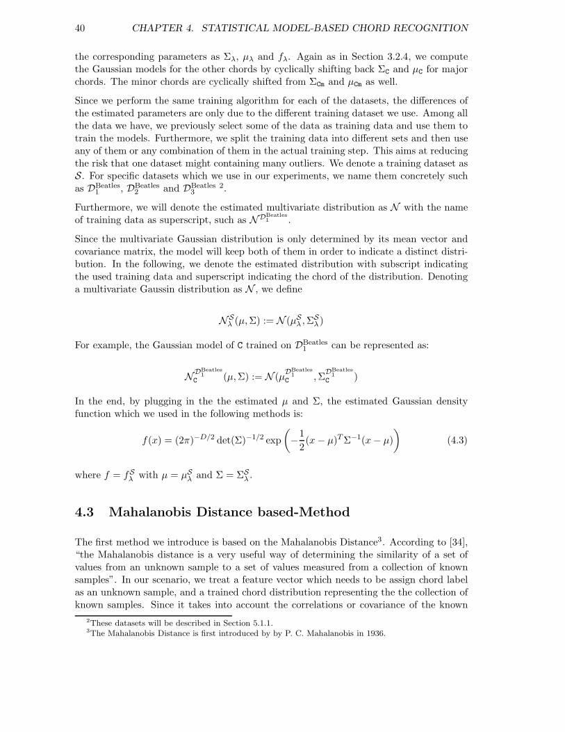
40 CHAPTER 4. STATISTICAL MODEL-BASED CHORD RECOGNITION
the corresponding parameters as Σλ, µλ and fλ. Again as in Section 3.2.4, we computethe Gaussian models for the other chords by cyclically shifting back ΣC and µC for majorchords. The minor chords are cyclically shifted from ΣCm and µCm as well.
Since we perform the same training algorithm for each of the datasets, the differences ofthe estimated parameters are only due to the different training dataset we use. Among allthe data we have, we previously select some of the data as training data and use them totrain the models. Furthermore, we split the training data into different sets and then useany of them or any combination of them in the actual training step. This aims at reducingthe risk that one dataset might containing many outliers. We denote a training dataset asS. For specific datasets which we use in our experiments, we name them concretely suchas DBeatles
1 , DBeatles2 and DBeatles
32.
Furthermore, we will denote the estimated multivariate distribution as N with the nameof training data as superscript, such as NDBeatles
1 .
Since the multivariate Gaussian distribution is only determined by its mean vector andcovariance matrix, the model will keep both of them in order to indicate a distinct distri-bution. In the following, we denote the estimated distribution with subscript indicatingthe used training data and superscript indicating the chord of the distribution. Denotinga multivariate Gaussin distribution as N , we define
N Sλ (µ,Σ) := N (µS
λ ,ΣSλ )
For example, the Gaussian model of C trained on DBeatles1 can be represented as:
NDBeatles
1
C (µ,Σ) := N (µDBeatles
1
C ,ΣDBeatles
1
C )
In the end, by plugging in the the estimated µ and Σ, the estimated Gaussian densityfunction which we used in the following methods is:
f(x) = (2π)−D/2 det(Σ)−1/2 exp
(
−1
2(x− µ)TΣ−1(x− µ)
)
(4.3)
where f = fSλ with µ = µS
λ and Σ = ΣSλ .
4.3 Mahalanobis Distance based-Method
The first method we introduce is based on the Mahalanobis Distance3. According to [34],“the Mahalanobis distance is a very useful way of determining the similarity of a set ofvalues from an unknown sample to a set of values measured from a collection of knownsamples”. In our scenario, we treat a feature vector which needs to be assign chord labelas an unknown sample, and a trained chord distribution representing the the collection ofknown samples. Since it takes into account the correlations or covariance of the known
2These datasets will be described in Section 5.1.1.3The Mahalanobis Distance is first introduced by by P. C. Mahalanobis in 1936.

4.3. MAHALANOBIS DISTANCE BASED-METHOD 41
distribution, it makes itself different from the Euclidean distance which only considersthe mean value. Furthermore, Mahalanobis Distance is scale-invariant [19] which meansit does not depend on the scale of measurement. This makes it more powerful whileanalyzing multivariate data.
While applying the Mahalanobis Distance on the chord recognition task, we make twoassumptions: the first one is that the distribution of our feature vectors should behaveas multivariate normal distribution of a random vector; the second one is that the dis-tributions of the 24 chords should be distinct among each other, otherwise it will yieldsame distance and make the chord undeterminable. For the first assumption, we checkthe distribution of practical data and find this assumption holds. For the second assump-tion, since we use the practical data to train the covariance matrix, and cyclically shiftthe ΣC and ΣCm to other major and minor chords, the covariance matrix of the 24 chordsare distinctive. Furthermore, the mean vector of each of all chords are different as well.Therefore the second assumption can be fulfilled.
4.3.1 Specification of Distance Measure
Definition 4.4 Let x be a feature vector, x ∈ F \ {0} and D be the dimension of F , andlet µ ∈ R
D be the mean value and Σ ∈ RD×D be the covariance matrix of a multivariate
normal distribution. Then, we define the Mahalanobis distance dM = dµ,SM : F × F → R
with respect to µ,Σ by
dM (x) =√
(x− µ)TΣ−1(x− µ) (4.4)
Typically, the matrix Σ must be semi-positive definite. Furthermore, if the matrix S isthe identity matrix, the Mahalanobis distance reduces to the Euclidean distance. If theΣ is diagonal, then the resulting distance measure reduces to the normalized Euclideandistance:
d(x) =
√
√
√
√
N∑
i=1
(x(i)− µ(i))2
σ(i)2, (4.5)
where σ(i) is the ith diagonal value of Σ.
4.3.2 Algorithm Procedure
After defining the trained models and distance measure, the chord recognition procedureusing Mahalanobis Distance can be described. Similar as in template-based methods, weneed to pass the feature sequence X := (x1, x2, . . . , xN ) which extracted from the audiofile in the following procedure.
• Firstly, the previously trained models describing the distribution of 24 chords areloaded. We take the mean vector and the covariance matrix from each of the chordmodels. Here ignoring the concrete training dataset for simplicity, suppose the ar-bitrary parameters which we load are µS
λ and ΣSλ

42 CHAPTER 4. STATISTICAL MODEL-BASED CHORD RECOGNITION
• Secondly, we take the Mahalanobis distance as a measurement to quantify the dis-tance between a feature vector and a chord distribution. By plugging in µS
λ and ΣSλ ,
we can measure the distance between xn and any of the chord distribution N Sλ (µ,Σ).
We denote the distance by dM (N Sλ (µ,Σ), xn).
• Finally, similar to template-based methods, we assign the chord label that minimizesthe distance between the corresponding distribution and the given feature vectorx = xn:
λxn := dMλ∈Λ
(N Sλ (µ,Σ), xn). (4.6)
4.4 Gaussian Probability based-Method
Instead of having similarity measured by distance function, we define a similarity mea-surement which allows the comparison of a feature with a Gaussian distribution. The ideais that given a distribution and a feature vector, we treat the feature vector as a samplevector and measure how possible the sample comes from the distribution. In other words,we can measure how possible that a feature vector fit the distribution of a chord pattern.In this way, we can quantify the relationship between a feature vector and a distributionby probability. In this section, we consider the case of multivariate Gaussian distributionand introduce the chord recognition method based on Gaussian probability.
Recall Equation (4.3) that the density function of Gaussian distribution is:
f(x) = (2π)−D/2 det(Σ)−1/2 exp
(
−1
2(x− µ)TΣ−1(x− µ)
)
For a given chord label λ ∈ Λ and a given training dataset S, we denote the densityfunction with f = fS
λ and the parameters as µ = µSλ and Σ = ΣS
λ .
Based on the formula we see that Gaussian probability is just the weighted exponentialform of the Mahalanobis Distance. One can even use the logarithm form so that it isdirectly related with the Mahalanobis Distance. Both of the methods are based on rel-ative comparison to select the maximum case (or minimum case in Mahalanobis) as therecognition result.
4.4.1 Algorithm Procedure
The chord recognition procedure using Gaussian Probability is the same as the procedureusing the Mahalanobis Distance in the first step, i.e., the step of loading the model param-eters. We make changes in the following steps, which correspond to the similarity measureand chord label assignment.
• To calculate the similarity, we take the Gaussian Probability as a measurement toquantify the possibility of a feature vector xn coming from a chord distributions N S
λ

4.5. HIDDEN MARKOV MODELS-BASED METHOD 43
corresponding to the chord label λ and training data set S. By plugging in theseparameters into fS
λ , we calculate all the probabilities for every λ ∈ Λ.
• In the end, the chord label is assigned to the feature vector x = xn by selecting theone whose model gets the maximum probability.
λxn := argminλ∈Λ
fSλ (xn). (4.7)
4.5 Hidden Markov Models-based Method
A Markov model is a stochastic model which fulfilles the Markov property. Accordingto [14], in a hidden Markov model (short form for HMM), “the output for each statecorresponds to an output probability distribution.” An HMM can be represented byits initial probability, observation probability and transition probability. Adapting theseparameters to chord recognition, we consider a chords as a hidden state in HMM, and afeature vector as an observation. The problem can be reformulated as given the sequenceof observations of features, what are the underlying states of chords which generate thefeature sequence. We use the Gaussian probability which we computed in the last sectionas observation probability, and train the transition probability from the training data.The initial probability is set to 1/24 indicating each of the chords has a fair chance.
The main idea of HMM-based chord recognition is to introduce temporal context into thechord recognition process. This can be seen as a kind of added post-filtering after theprimary pattern matching step. The post-filtering serves as smoothing of the predictedchord labels utilizing the context over time, in order to reduce wrong recognized framescaused by noise or strong onsets, and also to smooth fluctuating frames inside a continuedchord duration [4].
4.5.1 Transition Probability
In order to consider the temporal context, one needs a transition probability matrixA ∈ R
|Λ|×|Λ| for a given chord label set Λ. This matrix describes the first-order tem-poral relationships between the various chords. Each element of the matrix represents theprobability of a chord jumping to another. For example, A(λ1, λ2), λ1 6= λ2 represents theprobability chord λ1 jump to λ2, and A(λ1, λ1) represents the probability of staying in thesame chord λ1.
There are many ways to specify a transition probability matrix. Such a matrix may betrained from a training dataset, we denote the matrix with subscript t represent it is trained
and superscript the training data set, for example ADBeatles
1
t . For the matrix obtained fromtraining, we first parse the original label file into framewise labels with respect to the fixedfeature rate of 10 Hz, i.e., 10 labels per second with each of them indicating the chordlabel for 100 millisecond. To solve the rounding problem of time points which do not startor end sharply at hundred milliseconds, we take the ceiling of the time point when it isthe start of a label, while floor of the time point when it is the end of a label. Now we

44 CHAPTER 4. STATISTICAL MODEL-BASED CHORD RECOGNITION
have the labels for the whole training set with the unit of each hundred millisecond. Inthe end, the values of the element in the transition matrix is assigned to:
At(λ1, λ2) =C(λ1, λ2)∑
λ∈Λ
C(λ1, λ)(4.8)
where C(λ1, λ2) counts the number of chords jumping where the current label is λ1 andnext label is λ2, and
∑
C(λ1, λ) serves as a normalization which counts the jumping fromλ1 to all the labels including itself.
Another way of specifying the transition matrix is to set the value of its elements manuallyusing musical knowledge, we denote such a transition matrix as Am, with subscript mindicating it is manually set. For example, Bello and Pickens designed a figure of doubly-nested circle fifth to model the chord transition [3].
4.5.2 Viterbi Decoding
The Viterbi algorithm is a dynamic programming algorithm to find the most possiblesequence of underlying states of hidden Markov models given the sequence of observedevents. We use it to decode the hidden states of chords given the sequence of observedfeature vectors. In the following, part of the content is summarized from [14] and [31].
The Gaussian probability-based chord recognition as described in Section 4.4 is worked asthe observation probability in HMM. The observation probability describes if the currenthidden state is i, how likely it will lead to the observed event j. In the discrete form ofHMM, the observation probability of the states is usually discrete and fixed. However inthe implementation of our system, we need to adapt the HMM in its continuous form:instead of using a fixed value, the observation probability for a certain state is modeledby a specific Gaussian density function. Furthermore, we treat any given feature vectoras observed event and plug this vector into the density function. By doing this, as dis-cussed in Section 4.4, we calculate the probability of the vector coming from a certainchord distribution. This probability is then treated as the observation probability whichindicates the possibility that a chord state generates such a feature vector as observedevent. Certainly, this will lead to different possibilities for different feature vectors andtherefore make the observation probability unfixed and vary.
The HMM work out the most possible hidden states by using the Viterbi algorithm. TheViterbi algorithm combines both the observation probabilities and transition probabilitiesto perform post-filtering, i.e., based on the primary pattern matching result of chordlabel using Gaussian Probabilities, the Viterbi algorithm will determine the final resultconsidering the context influence specified by transition probabilities.
The idea of the Viterbi algorithm is a kind of dynamic programming which uses the statesat time t to deduct the optimal states at t + 1. It works recursively to find the optimalhidden states given the observation sequence and the parameters of HMM.
The algorithm runs in two stages. The first stage calculate the objective probability forany state at any time. Suppose we have M hidden states and we denote each state asSi, i ∈ [1 : M ]. We denote the observed events as Ot, t ∈ [1 : T ]. Then at an arbitrary

4.5. HIDDEN MARKOV MODELS-BASED METHOD 45
time point t, for each of the states Si, a partial probability δt(Si) is defined to indicate theprobability of the most probable path ending at the state Si, given the current observedevents O1, · · · , Ot:
δt(Si) = maxj
(δt−1(Sj) ·A(Sj , Si)) · P (Ot|Si) (4.9)
Here, we assume that we already know the probability δt−1(Sj) for any of the previousstates Sj at time t− 1, and using the transition probability of A(Sj , Si) and multiplyingit by the current observation probability P (Ot|Si). We then select the maximum δt(Si).
After having all the objective probabilities for each state at each time point, the algorithmseeks from the very end backwards to the beginning to find the most probable path ofstates for the given sequence of observation events.
φt(i) = argmaxj
(δt−1(Sj) · A(Sj , Si)) (4.10)
where φt(i) indicates which state is the most optimal state at time t based on the proba-bility computed in the first stage.

46 CHAPTER 4. STATISTICAL MODEL-BASED CHORD RECOGNITION

Chapter 5
Experiments
In this chapter we present the extensive experiments which we conducted to inspect the ef-fect of different stages of our chord recognition system. We depict the overall experimentalsetup in Section 5.1. In particular, the dataset including audio files and chord annotationswill be described in detail and the evaluation methodology will be introduced. In Sec-tion 5.2 we discuss the evaluation measures based on precision and recall. In Section 5.3,we conduct experiments on extracted features. Here, the optimization techniques such aslogarithmic compression, smoothing, pitch range separation will be extensively evaluated.Besides, we discuss the results of experiments and analyze certain effect. In Section 5.4,we do experiments on chord recognizers. Here, the six different chord recognizers as de-scribed in Chapter 3 and 4 will be extensively evaluated. We will point out the advantageand disadvantage of a certain recognition methods when combing with different features.From Section 5.5 to 5.8, experiments on other aspects will be introduced. We first presentthe effect of tuning and using different training data. Then, the impact of combining ourexisted chord recognition module with other techniques will be analyzed. These aspectsinclude harmonic-percussive source separation and using beat-wise features for evaluationinstead of frame-wise features.
5.1 Experiments Setup
5.1.1 Dataset
In this thesis, all the datasets we use consist of both audio files and corresponding chordannotation files which contain ground truth chord labels.
We prepared three different kinds of music data for our experiments. Firstly, we take theBeatles albums as representatives for pop music. We take all 180 songs as a whole dataset,and denote it as DBeatles. We further partition DBeatles into three subset, where all therecordings are ordered alphabetically and we put the first 60 recordings into DBeatles
1 , thesecond 60 recordings into DBeatles
2 , and the last 60 recordings into DBeatles3 . The chord
annotations for Beatles albums are written by Christopher Harte [13]. Secondly, we takethe four classical pieces as representatives for classical music. We put these four pieces
47

48 CHAPTER 5. EXPERIMENTS
together in a dataset and name it as D4. See Table 5.1 for details. The chord annotations inthis dataset are precisely written by Verena Konz. Furthermore, we particularly choose 16Beatles recordings and four classical pieces together as a combination of pop and classicalmusic. We name it as D20. See Table 5.2 for detail.
File ID File name (first 50 characters) Performer LengthBachBWV846Fischer Bach_BWV846_Fischer_22050_mono Fischer 84Beet5Bernstein Beethoven_op067_1_symphony_5_bernstein_22050_mono Bernstein 519ChopMazurkaSmith pid9054b-21 Smith 91SchumannKonz Schumann_Op068No4_Konz Konz 83
Table 5.1. Description of the dataset D4.
File ID File name (first 50 characters) Performer LengthBeatlesAHardDaysNight Beatles_AHardDaysNight_Beatles_1964-AHardDaysNigh Beatles 152BeatlesAllMyLoving Beatles_AllMyLoving_Beatles_1963-WithTheBeatles-0 Beatles 129BeatlesAllYouNeedIsLove Beatles_AllYouNeedIsLove_Beatles_1967-MagicalMyst Beatles 228BeatlesBoys Beatles_Boys_Beatles_1963-PleasePleaseMe-05 Beatles 147BeatlesDoYouWantToKnowASecret Beatles_DoYouWantToKnowASecret_Beatles_1963-Pleas Beatles 119BeatlesEightDaysAWeek Beatles_EightDaysAWeek_Beatles_1964-BeatlesForSal Beatles 165BeatlesGotToGetYouIntoMyLife Beatles_GotToGetYouIntoMyLife_Beatles_1966-Revolv Beatles 150BeatlesHelp Beatles_Help_Beatles_1965-Help-01 Beatles 141BeatlesHereComesTheSun Beatles_HereComesTheSun_Beatles_1969-AbbeyRoad-07 Beatles 185BeatlesLetItBe Beatles_LetItBe_Beatles_1970-LetItBe-06 Beatles 243BeatlesLovelyRita Beatles_LovelyRita_Beatles_1967-SgtPeppersLonelyH Beatles 162BeatlesLoveMeDo Beatles_LoveMeDo_Beatles_1963-PleasePleaseMe-08 Beatles 142BeatlesTicketToRide Beatles_TicketToRide_Beatles_1965-Help-07 Beatles 192BeatlesTwistAndShout Beatles_TwistAndShout_Beatles_1963-PleasePleaseMe Beatles 153BeatlesWhatGoesOn Beatles_WhatGoesOn_Beatles_1965-RubberSoul-08 Beatles 170BeatlesYesterday Beatles_Yesterday_Beatles_1965-Help-13 Beatles 127BachBWV846Fischer Bach_BWV846_Fischer_22050_mono Fischer 84Beet5Bernstein Beethoven_op067_1_symphony_5_bernstein_22050_mono Bernstein 519ChopMazurkaSmith pid9054b-21 Smith 91SchumannKonz Schumann_Op068No4_Konz Konz 83
Table 5.2. Description of the dataset D20.
5.1.2 Annotation Convention
In order to have a universal format of chord annotations, a certain rule is introduced byChristoph Harte in [13]. For the four classical pieces which we used, Verena Konz followedexactly the same rule when annotating the chords. Besides, the annotated chords areforced to map into one of the 24 triads when we parse the annotations. Here, we onlyconsider the first two intervals of each chord [16]. Thus, augmented chords are mappedto major and diminished chords are mapped to minor, respectively. In some cases, thereare regions where no chord exists. Such regions are annotated with “N” as annotation. Inour evaluation, we discard the regions where no chords exist, that is to say, whatever thecomputed result is in this region, it does not affect the recognition accuracy for the wholepiece.

5.2. EVALUATION VIA PRECISION AND RECALL 49
5.2 Evaluation via Precision and Recall
The evaluation measure of our chord recognition system is via precision and recall. Inparticular, we take F-measure, which is derived from precision and recall, as our recog-nition accuracy. In the field of information retrieval, precision and recall are defined asfollows [20].
precision =|{relevant documents} ∩ {retrieved documents}|
|{retrieved documents}|(5.1)
recall =|{relevant documents} ∩ {retrieved documents}|
|{relevant documents}|(5.2)
Adapt the concept into chord recognition, one can treat a chord label as a document.Therefore an annotated chord label can be seen as a relevant document and a computedchord label as a retrieved document. By plugging in both the label sequence of an audiofile into equation 5.1 and 5.2, one can calculate the F-measure as recognition accuracy [35]:
F = 2 ·precision · recall
precision + recall(5.3)
Note that our chord recognition system is based on framewise evaluation. All the chordannotations are segmented into frames with fixed length. The frame length depends onthe feature rate which is always 10 in our experimental setting. The number of segmentedannotation frames corresponds to the number of computed chord label frames, whichequals to the number of feature frames.
5.3 Experiments on Extracted Features
From this section on, we discuss the extensive experiments which we conducted. In Chap-ter 2 we have introduced several features which transform the original audio files intomusically meaningful representations, in particular, all of them are in the chroma repre-sentation. These features are then passed into the chord recognition module which makechord label decisions via classification based on some template methods or statistical mod-els. To understand which influence the features make to the whole process, we conductseries of experiments in this section that mainly focus on the feature side. We evaluatethe performance variations by using all the features with different setting of parameters,so that we can explore the effect of parameters. From the difference of the performanceresults, we can clearly discover how these feature settings increase or decrease the chordrecognition accuracies. Moreover, we can infer the advantage and the disadvantage ofusing a certain type of feature when combining it with different chord recognizers.
This section is structured as follows. Section 5.3.1 illustrates the overall performance of thecombinations of all features and recognizers. We provide two sets of results with differenttraining datasets so that we can deduct the feature performance more generally than

50 CHAPTER 5. EXPERIMENTS
using a single dataset. Section 5.3.3 illustrates the influence of logarithmic compressionon the magnitude of loudness. With different extents of compression, we will see thechanges in the chromagram and changes in the recognition result as well. By enlargingthe window size when computing the CENS and CRP, we examine how smoothing affectsthe final performance in the Section 5.3.4. Finally, Section 5.3.5 discuss the pitch rangeseparation in order to observe the different behavior of features extracted from only themelody part or the bass part of a piece of music.
5.3.1 Overall Performance
As the first introductive experiment, we provide the overall recognition accuracies of ourchord recognition system with all feature types and all chord recognition methods. Theparameters of the features are selected to be the optimal ones in this overall illustration.Here we use DBeatles as the test dataset so that we can compare the performance of oursystem to the ones in other groups. Note that recognition accuracies of the two recognitionmethods Tb and Th only depend on the test dataset while the recognition accuracies ofother other four methods depend on both the test dataset and the training dataset. Inorder to alleviate the possible effect of unfair training, we provide two tables of resultswith each trained on different datasets respectively.
Table 5.3 shows the evaluation result of chord recognition for the five feature types andfor six chord recognition methods with some of them previously trained on the datasetDBeatles
1 and all of them tested on DBeatles. The rows of the table change the chordrecognizer in turn and the columns change the features in turn. In order to have a bettervisualization of the performance result, we provide the bar figure corresponding to thevalues of Table 5.3 in Figure 5.1. From both the table and the figure we can find thatCP performs the worst with almost all chord recognizers except with Tb. This makessense since CP is the most basic chroma feature without any additional processing suchas smoothing, or logarithmic compression. Feature CLP(1000) performs quite well andcan be considered as the second best feature. For all the chord recognizers except Maha,feature CLP(1000) wins the second place. (Here for HMM, CLP(1000) got 0.717 and CISP
got 0.714, we ignore this small difference and consider both of them win the second place.)Feature CISP behaves very strange: it performs excellent with HMM but defective withother chord recognizers. It got one time the worst feature with Tb, three times the secondworst place with Th Ta GP. This indicates that CISP depends very much on smoothing.Furthermore, its bad performance with Tb indicates that its magnitude computation is notthat emphasizing the component note of the chord but gives extra weight to other notes.Feature CENS(13, 1) can be considered as a fair feature and wins the middle place amongthe five feature types. Note that it already contains quantization on magnitude, whichworks similar to logarithmic compression at the feature side. Additionally, smoothing isalso included when giving the window size 13 which in this case equals to 1.3 seconds.Although it includes both the optimization techniques, it is still worse than CLP(1000)for most of the recognizers. This indicates that the magnitude computation of a singlefeature is more important than smoothing with context. However, this does not mean thatsmoothing is not important. Without smoothing, CENS behaves quite unsatisfiable. Wewill discuss this in Section 5.3.4. At last comes the winner feature CRP(13, 1). It wins the

5.3. EXPERIMENTS ON EXTRACTED FEATURES 51
first place with all the chord recognizers. As we described in Chapter 2, the CRP featureis designed to boost timbre invariance. Besides, it contains the logarithmic compressionas CLP and smoothing as CENS. The combination of these techniques makes it prominentand outstanding among all features.
From Table 5.3 we can already tell the huge recognition difference caused by feature side.For all the chord recognizers, the best feature is always the CRP(13, 1) and the worst isCP for most of the time and CISP for one time. And for each of the recognizers, thebiggest increased recognition accuracy is 0.20, 0.31, 0.25, 0.34, 0.26 and 0.21 respectively.This implies the importance of computing audio features in a suitable way. Without goodfeatures, one can not obtain satisfiable result even using the complex chord recognizers.
CR CP CLP(1000) CISP CENS(13, 1) CRP(13, 1)
Tb 0.460 0.541 0.429 0.551 0.620
Th 0.342 0.590 0.467 0.530 0.653
Ta 0.422 0.601 0.481 0.566 0.675
Maha 0.331 0.388 0.425 0.526 0.672
GP 0.429 0.611 0.504 0.581 0.683
HMM 0.528 0.714 0.717 0.644 0.730
Table 5.3. Recognition accuracies of all features and all recognition methods. Train: DBeatles1
.Test: DBeatles.
Tb Th Ta0.3
0.35
0.4
0.45
0.5
0.55
0.6
0.65
0.7
0.75
(a) Template-based methods
Maha Gauss HMM 0.3
0.35
0.4
0.45
0.5
0.55
0.6
0.65
0.7
0.75
CPCLP(1000)CISPCENS(13,1)CRP(13,1)
(b) Statistical model-based methods
Figure 5.1. Bar visualization of Table 5.3. Result comparison from feature side.
Table 5.4 shows the evaluation result as well but using training dataset DBeatles2 . Since
Tb and Th do not include training procedure, the results of the both methods stays thesame as in Table 5.3. By comparing the two tables, we can find that most of the valueswhich locate at the same position of the two tables have only small differences below 0.030,except for the feature CLP(1000) with Maha surprisingly yield the biggest difference 0.105,and second biggest at CLP(1000) with HMM yield the difference 0.035. The later value iseven being the highest recognition accuracies among the two tables. From this we concludethat except feature CLP(1000), all other features are not that sensitive to the variations oftraining data, and the feature CLP(1000) is comparably sensitive than the other features.

52 CHAPTER 5. EXPERIMENTS
CR CP CLP(1000) CISP CENS(13, 1) CRP(13, 1)
Tb 0.460 0.541 0.429 0.551 0.620
Th 0.342 0.590 0.467 0.530 0.653
Ta 0.419 0.607 0.484 0.568 0.670
Maha 0.387 0.493 0.453 0.556 0.681
GP 0.411 0.621 0.496 0.562 0.660
HMM 0.525 0.749 0.717 0.639 0.710
Table 5.4. Recognition accuracies of all features with all recognition methods. Train: DBeatles2
.Test: DBeatles.
5.3.2 Feature Comparison
In this section, we compare features by visualizing all of the features extracted from thesame audio file. We excerpt the first ten seconds from the song BeatlesLetItBe forillustration. Figure 5.2 shows the intensity difference of chromagrams among five differentfeatures on the left side. Then for each of the feature type, we pass the features to thetemplate baseline method and get the corresponding recognition result. The visualizationof these results and the recognition accuracy are shown on the right side of Figure 5.2. Theimage range of the chromagrams for feature CP, CLP(1000), CISP and CENS(13, 1) are set to[0, 1] for easy comparison, while for feature CRP(13, 1) the range is [−0.7, 0.7] because CRPfeatures have negative intensity and the the range [−0.7, 0.7] yields a good visualization.For the result visualizations, the four different colors have a specific meaning: green meansannotated ground truth chords, red means computed chords but not coincide with groundtruth annotation, blue means computed chords and coincide with ground truth annotation,white means no annotations.
By comparing the color intensity of chromagrams, we can compare the magnitude orenergy of different feature types. We find that CLP(1000) and CISP share very similarcontrast in intensity, CP and CENS(13, 1) are to some extent similar as well. Althoughthe intensity contrast of CRP(13, 1) is higher than other features, by careful observationwe find the red highlight chromas and their time position are very close to the blue oryellow highlight chromas in CLP. Therefore we can roughly divide the five feature typesinto two groups by similarity of contrast: one is CLP(1000),CISP and CRP(13, 1); the otheris CP and CENS(13, 1). Actually this similarity of contrast makes sense because it reflectsthe different intensity computation of the chromagrams. On one hand, for feature CP
and CENS(13, 1), the intensity is in the form of energy, that is to say, the squared powerof amplitude of the original signal. Here squared power implies that, the difference ofintensity will be much enlarged after squaring the original value. On the other hand, forCISP, the intensity is in the form of magnitude, which derived from fourier transformation,and can be considered as the scaled amplitude of the original signal. For CLP(1000) andCRP(13, 1), the intensity of the both features are in the manner of energy, however theyperform logarithmic compression on the energy afterwards while computing the intensity,therefore the effect of squared power is to some extent cancel out. This yields the intensity

5.3. EXPERIMENTS ON EXTRACTED FEATURES 53
of chromagram in a manner between energy or magnitude. This is also the reason whythe chromagrams of CLP(1000) and CRP(13, 1) have less contrast than CP and CENS(13, 1).
The logarithmic compression in energy actually plays an important role in the chordrecognition task. This is because when speaking of a single chord, we give all componentnotes of this chord the same weight. Given the sheet music, we can decide the chordswithout any magnitude information from the played notes. Therefore the informationof magnitude difference of component notes is not that useful in chord recognition task.For example, from 5.9 to 6.8 seconds of BeatlesLetItBe, the ground truth annotation is“F:maj6” and after mapping to triad chord it becomes F. In Figure 5.2, only CLP and CRP
correctly recognize this period while the other features make wrong decision to Dm. Frommusical point of view, the error makes sense because “F:maj6” consists of the componentnotes F, A, C and D. They can either be mapped to F which is composed of F, A andC; or be mapped to D which is composed of D, F and A. In Figure 5.2(b) and 5.2(h), wecan find that CP and CENS have a high weight for chroma D from 5.9 to 6.8 seconds, thisdirectly leads to the wrong recognition of Dm instead of the correct F.
Another important factor is the smoothing effect. For the features without temporalsmoothing, their behavior is comparably unstable than the features with smoothing. Theyhave such disadvantage in particular for the case when the duration of a chord last fora long time. For example, from 4.7 to 4.9 seconds of BeatlesLetItBe, feature CP, CLPand CISP all wrongly recognize the chord as C due to the presence of the additional noteG in the chord Am. However with smoothing window length 13, feature CENS and CRP
successfully stay in Am because the contribution of note G is reduced when blending withthe strong Am context. This is also the main advantage of features with smoothing to gaina higher recognition accuracy than those without smoothing especially for long lastingchords.
From the comparison among different features we conclude the positive effect of logarith-mic compression and smoothing, however these two techniques also have limitations andsometimes yield negative effects. We will analyze this in detail in the following sections.

54 CHAPTER 5. EXPERIMENTS
(a) Score of the first 10 seconds (corresponding to the first threemeasures) of BeatlesLetItBe.
0 1 2 3 4 5 6 7 8 9
C
C#
D
D#
E
F
F#
G
G#
A
A#
B
0
0.1
0.2
0.3
0.4
0.5
0.6
0.7
0.8
0.9
1
(b) CP
0 1 2 3 4 5 6 7 8 9 C
C#/Db D
D#/Eb E/Fb E#/F
F#/Gb G
G#/Ab A
A#/Bb B/Cb
cc#/db
dd#/eb
e/fb e#/ff#/gb g
g#/ab a
a#/bb b/cb
0
0.5
1
1.5
2
2.5
3
(c) Recognition accuracy 0.820
0 1 2 3 4 5 6 7 8 9
C
C#
D
D#
E
F
F#
G
G#
A
A#
B
0
0.1
0.2
0.3
0.4
0.5
0.6
0.7
0.8
0.9
1
(d) CLP(1000)
0 1 2 3 4 5 6 7 8 9 C
C#/Db D
D#/Eb E/Fb E#/F
F#/Gb G
G#/Ab A
A#/Bb B/Cb
cc#/db
dd#/eb
e/fb e#/ff#/gb g
g#/ab a
a#/bb b/cb
0
0.5
1
1.5
2
2.5
3
(e) Recognition accuracy 0.870
0 1 2 3 4 5 6 7 8 9
C
C#
D
D#
E
F
F#
G
G#
A
A#
B
0
0.1
0.2
0.3
0.4
0.5
0.6
0.7
0.8
0.9
1
(f) CISP
0 1 2 3 4 5 6 7 8 9 C
C#/Db D
D#/Eb E/Fb E#/F
F#/Gb G
G#/Ab A
A#/Bb B/Cb
cc#/db
dd#/eb
e/fb e#/ff#/gb g
g#/ab a
a#/bb b/cb
0
0.5
1
1.5
2
2.5
3
(g) Recognition accuracy 0.770
0 1 2 3 4 5 6 7 8 9
C
C#
D
D#
E
F
F#
G
G#
A
A#
B
0
0.1
0.2
0.3
0.4
0.5
0.6
0.7
0.8
0.9
1
(h) CENS(13, 1)
0 1 2 3 4 5 6 7 8 9 C
C#/Db D
D#/Eb E/Fb E#/F
F#/Gb G
G#/Ab A
A#/Bb B/Cb
cc#/db
dd#/eb
e/fb e#/ff#/gb g
g#/ab a
a#/bb b/cb
0
0.5
1
1.5
2
2.5
3
(i) Recognition accuracy 0.850
0 1 2 3 4 5 6 7 8 9
C
C#
D
D#
E
F
F#
G
G#
A
A#
B
−0.6
−0.4
−0.2
0
0.2
0.4
0.6
(j) CRP(13, 1)
0 1 2 3 4 5 6 7 8 9 C
C#/Db D
D#/Eb E/Fb E#/F
F#/Gb G
G#/Ab A
A#/Bb B/Cb
cc#/db
dd#/eb
e/fb e#/ff#/gb g
g#/ab a
a#/bb b/cb
0
0.5
1
1.5
2
2.5
3
(k) Recognition accuracy 0.890
Figure 5.2. Comparisons of features and their recognition accuracies using chord recognizer Tb.
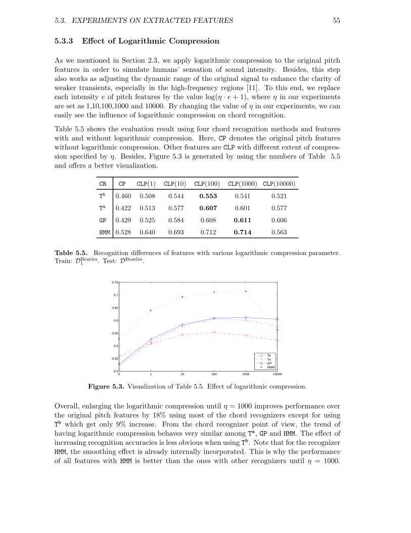
5.3. EXPERIMENTS ON EXTRACTED FEATURES 55
5.3.3 Effect of Logarithmic Compression
As we mentioned in Section 2.3, we apply logarithmic compression to the original pitchfeatures in order to simulate humans’ sensation of sound intensity. Besides, this stepalso works as adjusting the dynamic range of the original signal to enhance the clarity ofweaker transients, especially in the high-frequency regions [11]. To this end, we replaceeach intensity e of pitch features by the value log(η · e + 1), where η in our experimentsare set as 1,10,100,1000 and 10000. By changing the value of η in our experiments, we caneasily see the influence of logarithmic compression on chord recognition.
Table 5.5 shows the evaluation result using four chord recognition methods and featureswith and without logarithmic compression. Here, CP denotes the original pitch featureswithout logarithmic compression. Other features are CLP with different extent of compres-sion specified by η. Besides, Figure 5.3 is generated by using the numbers of Table 5.5and offers a better visualization.
CR CP CLP(1) CLP(10) CLP(100) CLP(1000) CLP(10000)
Tb 0.460 0.508 0.544 0.553 0.541 0.521
Ta 0.422 0.513 0.577 0.607 0.601 0.577
GP 0.429 0.525 0.584 0.608 0.611 0.606
HMM 0.528 0.640 0.693 0.712 0.714 0.563
Table 5.5. Recognition differences of features with various logarithmic compression parameter.Train: DBeatles
1. Test: DBeatles.
0 1 10 100 1000 100000.4
0.45
0.5
0.55
0.6
0.65
0.7
0.75
TbTaGPHMM
Figure 5.3. Visualization of Table 5.5. Effect of logarithmic compression.
Overall, enlarging the logarithmic compression until η = 1000 improves performance overthe original pitch features by 18% using most of the chord recognizers except for usingTb which get only 9% increase. From the chord recognizer point of view, the trend ofhaving logarithmic compression behaves very similar among Ta, GP and HMM. The effect ofincreasing recognition accuracies is less obvious when using Tb. Note that for the recognizerHMM, the smoothing effect is already internally incorporated. This is why the performanceof all features with HMM is better than the ones with other recognizers until η = 1000.

56 CHAPTER 5. EXPERIMENTS
However, it seems that just due to this smoothing effect, when η = 10000 the HMM has asharper decrease than other recognizers.
The best compression parameters for template-based methods (η = 100) and for statistical-model-based methods (η = 1000) are not the same. However, the result difference of usingη = 100 or η = 1000 is quite small, which is less than 1%. Enlarging the logarithmiccompression to 10000, the recognition accuracies of all the chord recognizers decrease.This indicates the optimal compression parameter lies in the range [100, 1000].
In order to further inspect the effect of logarithmic compression on features, the chroma-grams of features with or without different logarithmic parameters are shown in Figure 5.4.From 0 to 1.8 seconds, the chroma G gets much more obvious as the enlarging the com-pression parameter, while at the same time the chroma C gets less obvious yet still clearlyvisible. This assists the chord recognizers to determine the correct chord C since the weightsof both the components notes are the same in Tb. However, for some cases, logarithmiccompression also brings a negative effect. For example, at around 3.4 to 3.5 second, thechord changes from G to Am. In the chromagrams of feature CP and CLP(1), the intensityof chroma G is very weak, and the chroma A, E and C are strong in contrast to G. Thechord edge is sharp and clear so that the following recognizers will make correct decisionsabout the time point when chord changes. But in the chromagrams of feature CLP(1000),the chroma G and chroma A nearly have the same intensity. With the presence chroma ofC and E, it is hard for the following chord recognizers to decide whether the correct chordshould be C which consists of C,E and G, or should be Am which consists of A, C and E.In other words, the edge of chord changes are blurred in this way. This is also the reasonthat CLP(1000) is wrong at this time position but CP avoids this error in Figure 5.2.
0 1 2 3 4 5 6 7 8 9
C
C#
D
D#
E
F
F#
G
G#
A
A#
B
0
0.1
0.2
0.3
0.4
0.5
0.6
0.7
0.8
0.9
1
(a) CP
0 1 2 3 4 5 6 7 8 9
C
C#
D
D#
E
F
F#
G
G#
A
A#
B
0
0.1
0.2
0.3
0.4
0.5
0.6
0.7
0.8
0.9
1
(b) CLP(1)
0 1 2 3 4 5 6 7 8 9
C
C#
D
D#
E
F
F#
G
G#
A
A#
B
0
0.1
0.2
0.3
0.4
0.5
0.6
0.7
0.8
0.9
1
(c) CLP(10)
0 1 2 3 4 5 6 7 8 9
C
C#
D
D#
E
F
F#
G
G#
A
A#
B
0
0.1
0.2
0.3
0.4
0.5
0.6
0.7
0.8
0.9
1
(d) CLP(100)
0 1 2 3 4 5 6 7 8 9
C
C#
D
D#
E
F
F#
G
G#
A
A#
B
0
0.1
0.2
0.3
0.4
0.5
0.6
0.7
0.8
0.9
1
(e) CLP(1000)
0 1 2 3 4 5 6 7 8 9
C
C#
D
D#
E
F
F#
G
G#
A
A#
B
0
0.1
0.2
0.3
0.4
0.5
0.6
0.7
0.8
0.9
1
(f) CLP(10000)
Figure 5.4. Comparisons of different logarithmic compression on chroma features.

5.3. EXPERIMENTS ON EXTRACTED FEATURES 57
5.3.4 Effect of Smoothing
In this section we evaluate the impact of the smoothing at the feature side on the chordrecognition performance. Among all the feature types, we only integrated smoothingparameter in CENS and CRP. As we described in Section 2.4 and 2.5, we convolve eachsingle feature vector x with the neighbor feature vectors which are within a Hann windowof fixed length w centered on x. Here w specifies the number of the neighbor featurevectors and therefore control the size of smoothing. For the chord recognition methodswhich require training, the models are retrained using features with the specified smoothingwindow length w as in the evaluation.
The evaluation results of smoothing using CENS features are shown in Figure 5.5. Recallthat for CENS features, CENS(w, d) means we use the smoothing window size w and down-sampling factor d. Here we have no down-sampling at all therefore set d = 1 in all theexperiments. On the contrary, w is enlarging so that the extent of smoothing is rising.Note that by setting w = 1, CENS(1, 1) simply means no smoothing.
In general, the best smoothing result of CENS(w, 1) feature improves performance over thenon smoothing CENS(1, 1) by 22%, 16%, 15% and 3% for chord recognizer Tb, Ta, GP andHMM respectively. The best results come from the w = 25 for all recognizers except forHMM where w = 15. Furthermore, from Figure 5.5 we can see that the overall trend of allrecognizers except HMM are quite similar as well. As w is getting larger, the recognitionaccuracies of all chord recognizers get higher. In particular, increasing w from 1 to 3 getsthe most rapid increase in accuracies. For HMM, the reason that it behaves differently fromother recognizers is that HMM already integrated post-smoothing due to its internal viterbidecoding algorithm which emphasizes the situation of a chord staying in itself. Therefore,in this experiment it actually contains two stages of smoothing: both on the feature sideand on the recognizer side. This makes HMM distinct from other recognizers.
Similar to CENS features, we test the smoothing effect on CRP features as well. Figure 5.6illustrates the results. The smoothing also improves the recognition accuracies as weincrease the window length. However, the extent of increase is not as large as on CENS
features. CRP reaches the optimum with w = 21 which is smaller than the w = 25 for CENSand the increase is 10%, 10%, 11% for the first three recognizers. To our surprise, there isnearly no improvement of using HMM, where the difference between the optimal CRP(13, 1)and CRP(1, 1) is only 0.2%.
Figure 5.7 shows the chromagrams of CENS(w, 1) with different settings of w and thecorresponding chord recognition visualization for the first 10 seconds of BeatlesLetItBe.By comparing the recognition accuracy, we find that smoothing works as double-edgedsword: on one hand, it smoothes out the error and thus increases the accuracy, on theother hand, it also smoothes out the correct answer and decreases the accuracy. Figure 5.7reflects this phenomenon obviously: from 4.8 to 5.0 seconds the error occurs for CENS(1, 1)but is smoothed out for CENS(9, 1). This is because that at the time point of 4.8 secondin CENS(1, 1), the chroma A has nearly zero intensity in CENS(1, 1), and the chroma G haslow intensity yet it is larger then zero. In CENS(9, 1) with the smoothing effect, at thattime point since A gets larger intensity while G gets smaller since its neighbor featurescontain no intensity of G. However, from 5.1 to 5.6 seconds, some correct recognized F

58 CHAPTER 5. EXPERIMENTS
1 3 5 7 9 11 13 15 17 19 21 23 25
0.35
0.4
0.45
0.5
0.55
0.6
0.65
0.7
stat window length
Acc
urac
y
TbTaGPHMM
CR Tb Ta GP HMM
CENS(1, 1) 0.345 0.426 0.442 0.580CENS(3, 1) 0.428 0.472 0.479 0.591CENS(5, 1) 0.465 0.499 0.503 0.597CENS(7, 1) 0.491 0.520 0.522 0.604CENS(9, 1) 0.511 0.537 0.540 0.610CENS(11, 1) 0.525 0.551 0.555 0.613CENS(13, 1) 0.536 0.563 0.566 0.615CENS(15, 1) 0.546 0.570 0.575 0.616CENS(17, 1) 0.553 0.576 0.581 0.615CENS(19, 1) 0.558 0.580 0.585 0.614CENS(21, 1) 0.562 0.584 0.588 0.613CENS(23, 1) 0.565 0.586 0.591 0.610CENS(25, 1) 0.567 0.587 0.592 0.608
Figure 5.5. Recognition accuracies of using different smoothing window length in CENS features.Train: DBeatles
1 . Test: DBeatles3 .
1 3 5 7 9 11 13 15 17 19 21 23 250.52
0.54
0.56
0.58
0.6
0.62
0.64
0.66
0.68
0.7
0.72
stat window length
Acc
urac
y
TbTaGPHMM
CR Tb Ta GP HMM
CRP(1, 1) 0.523 0.574 0.580 0.713CRP(3, 1) 0.551 0.604 0.611 0.714CRP(5, 1) 0.571 0.625 0.632 0.715CRP(7, 1) 0.586 0.641 0.648 0.715CRP(9, 1) 0.598 0.652 0.660 0.714CRP(11, 1) 0.607 0.661 0.671 0.714CRP(13, 1) 0.613 0.667 0.677 0.715CRP(15, 1) 0.617 0.671 0.683 0.715CRP(17, 1) 0.622 0.672 0.686 0.713CRP(19, 1) 0.624 0.674 0.689 0.712CRP(21, 1) 0.625 0.674 0.691 0.711CRP(23, 1) 0.625 0.673 0.691 0.708CRP(25, 1) 0.624 0.672 0.691 0.703
Figure 5.6. Recognition accuracies of using different smoothing window length in CRP features.Train: DBeatles
1. Test: DBeatles
3.
was smoothed out to the wrong chord Am. This is because in CENS(1, 1), at that shorttime, chroma F is originally stronger than A which yields the correct chord F. But aftersmoothing with the neighbors, chroma F gets weaker than A, because in the neighborfeatures the intensity of F is less than A.
When w is increased to 21, which means each feature is blend with 2.1 seconds of theoriginal audio file, we find that the error which occurs in all other CENS features withsmaller w from 6 to 7 second totally disappears in CENS(21, 1). But such large w alsoblurs the edge of the chord transition. We find that nearly all the start and end of thechord transition is wrong in CENS(21, 1). However when w is less than 9, the edge can beperfectly recognized.

5.3. EXPERIMENTS ON EXTRACTED FEATURES 59
(a) Score of the first 10 seconds (corresponding to the first threemeasures) of BeatlesLetItBe.
0 1 2 3 4 5 6 7 8 9
C
C#
D
D#
E
F
F#
G
G#
A
A#
B
0
0.1
0.2
0.3
0.4
0.5
0.6
0.7
0.8
0.9
1
(b) CENS(1, 1)
0 1 2 3 4 5 6 7 8 9 C
C#/Db D
D#/Eb E/Fb E#/F
F#/Gb G
G#/Ab A
A#/Bb B/Cb
cc#/db
dd#/eb
e/fb e#/ff#/gb g
g#/ab a
a#/bb b/cb
0
0.5
1
1.5
2
2.5
3
(c) Recognition accuracy 0.850
0 1 2 3 4 5 6 7 8 9
C
C#
D
D#
E
F
F#
G
G#
A
A#
B
0
0.1
0.2
0.3
0.4
0.5
0.6
0.7
0.8
0.9
1
(d) CENS(5, 1)
0 1 2 3 4 5 6 7 8 9 C
C#/Db D
D#/Eb E/Fb E#/F
F#/Gb G
G#/Ab A
A#/Bb B/Cb
cc#/db
dd#/eb
e/fb e#/ff#/gb g
g#/ab a
a#/bb b/cb
0
0.5
1
1.5
2
2.5
3
(e) Recognition accuracy 0.820
0 1 2 3 4 5 6 7 8 9
C
C#
D
D#
E
F
F#
G
G#
A
A#
B
0
0.1
0.2
0.3
0.4
0.5
0.6
0.7
0.8
0.9
1
(f) CENS(9, 1)
0 1 2 3 4 5 6 7 8 9 C
C#/Db D
D#/Eb E/Fb E#/F
F#/Gb G
G#/Ab A
A#/Bb B/Cb
cc#/db
dd#/eb
e/fb e#/ff#/gb g
g#/ab a
a#/bb b/cb
0
0.5
1
1.5
2
2.5
3
(g) Recognition accuracy 0.850
0 1 2 3 4 5 6 7 8 9
C
C#
D
D#
E
F
F#
G
G#
A
A#
B
0
0.1
0.2
0.3
0.4
0.5
0.6
0.7
0.8
0.9
1
(h) CENS(13, 1)
0 1 2 3 4 5 6 7 8 9 C
C#/Db D
D#/Eb E/Fb E#/F
F#/Gb G
G#/Ab A
A#/Bb B/Cb
cc#/db
dd#/eb
e/fb e#/ff#/gb g
g#/ab a
a#/bb b/cb
0
0.5
1
1.5
2
2.5
3
(i) Recognition accuracy 0.850
0 1 2 3 4 5 6 7 8 9
C
C#
D
D#
E
F
F#
G
G#
A
A#
B
0
0.1
0.2
0.3
0.4
0.5
0.6
0.7
0.8
0.9
1
(j) CENS(17, 1)
0 1 2 3 4 5 6 7 8 9 C
C#/Db D
D#/Eb E/Fb E#/F
F#/Gb G
G#/Ab A
A#/Bb B/Cb
cc#/db
dd#/eb
e/fb e#/ff#/gb g
g#/ab a
a#/bb b/cb
0
0.5
1
1.5
2
2.5
3
(k) Recognition accuracy 0.870
0 1 2 3 4 5 6 7 8 9
C
C#
D
D#
E
F
F#
G
G#
A
A#
B
0
0.1
0.2
0.3
0.4
0.5
0.6
0.7
0.8
0.9
1
(l) CENS(21, 1)
0 1 2 3 4 5 6 7 8 9 C
C#/Db D
D#/Eb E/Fb E#/F
F#/Gb G
G#/Ab A
A#/Bb B/Cb
cc#/db
dd#/eb
e/fb e#/ff#/gb g
g#/ab a
a#/bb b/cb
0
0.5
1
1.5
2
2.5
3
(m) Recognition accuracy 0.900
Figure 5.7. Comparisons of different window lengths of smoothing on CENS features. Test onrecognizer Tb and test data : the first 10 seconds of BeatlesLetItBe.

60 CHAPTER 5. EXPERIMENTS
The next question is what the optimal value for w is. Although CENS(21, 1) yields thehighest recognition accuracy of 0.90 among all the settings, does it really make sense tohave such a large smoothing window which blend in the original signal more than twoseconds? The answer to that question is, that there is no universal optimal value since thedurations of the chord differ for each song. For some of the music pieces which containArpeggio such as Bach BWV846, it would be good to have a large window than thecommon pieces of music since the notes of the chords are separately played. While forsome of the pop music in which the duration of chords are short and the chords rapidlychange, it would be good to have a small window. However, in general, we consider thatthe window size corresponding to 0.5 second does make sense, since most of the chordslast at least 0.5 second.
5.3.5 Effect of Pitch Range Separation
In this section we evaluate the effect of pitch range separation by dividing the whole pitchrange p ∈ [1 : 120] to some smaller range mainly representing melody and bass. We usetwo types of features in our evaluation. One is CISP, the other is CRP.
Pitch Range Separation for CLP :
In CISP features, the melody part is restricted to p ∈ [43 : 92] covering musical notes fromG2 to G6, and the bass part is in p ∈ [21 : 68] covering notes from A0 to A4. Note thereis an overlap range in the two parts. Furthermore, in order to test the effect of usingmore dimensions other than 12 to represent the chromas, here we combine both the 12dimensional melody range features and the 12 dimensional bass range features verticallyto form 24 dimensional features.
Table 5.6 shows the evaluation results of using CISP features. The first column whichis named “12dim all” is the normal CISP we used in other experiments. From the tablewe see that the general performance of using melody range features is very close to theperformance of using whole range features. The biggest recognition difference between thetwo types of features is only 1.5% at recognizer Tb. However, using bass range featuresdramatically decreases the performance. The recognition decreases from 7% to 15% com-pared to the features using the whole range. The biggest difference comes from Tb as well.This implies that the melody pitch range is more or less able to cover the pitch of mostplayed notes in the dataset, while the bass pitch range captures only several played notesand misses most notes who have higher pitches.
For the comparison of dimensions of features, we find that the results of using 24 dimen-sions and using 12 dimensions are very close to each other as well. For Tb and GP, the24 dimensional features increase the accuracy about 1%. For Ta and HMM, the accuracy isdecreased, but only less than 1%.
Pitch Range Separation for CLP :
Table 5.7 shows the pitch range separation results using CLP features. First we focus onthe 12 dimensional features which are in the first three columns. Different from using CISPfeatures, the recognition accuracy of the melody range features is 5% to 7% less than thenormal whole range features for all the CLP with Tb. For other recognitions, the difference

5.3. EXPERIMENTS ON EXTRACTED FEATURES 61
CR 12dim all 12dim melody 12dim bass 24dim all
Tb 0.429 0.414 0.279 0.441
Ta 0.481 0.472 0.406 0.475
GP 0.504 0.495 0.399 0.514
HMM 0.717 0.703 0.642 0.715
Table 5.6. Recognition differences of pitch range separation of CISP. Train: DBeatles1 . Test:
DBeatles.
between them is also larger than those tested on CISP features. A common phenomenonoccurs in both CLP and sCISP is the bad performance of using bass range features. Againwe get about 7% to 20% decrease.
For the dimension comparison of CLP, the result varies with different compression param-eters. For CLP(1), the “24dim all” features improves recognition at most 5% and at least2%. However, this improvement becomes less and less as the log compression parameter ηgets larger. Until η = 100 it still improves the result. But to our surprise, when η = 100,it decreases the result of GP by 30% and HMM by 35%, while it stays nearly the same for Tb
and Ta. This is because for large compression parameters, the intensity difference betweenchromas is already quite small and hard to distinguish, now putting such undistinguishedchroma features into a complex model, the model pattern we learned will be even moreundistinguished among each of the chords. That is why for the template method theperformance is still ok but for complex methods it totally fails.
CR 12dim 12dim 12dim 24dimall melody bass all
Tb 0.508 0.455 0.397 0.551Ta 0.513 0.475 0.353 0.545GP 0.541 0.490 0.508 0.582HMM 0.665 0.623 0.599 0.686
CR 12dim 12dim 12dim 24dimall melody bass all
Tb 0.544 0.487 0.396 0.572Ta 0.577 0.535 0.382 0.585GP 0.601 0.552 0.535 0.632HMM 0.710 0.675 0.631 0.727
CR 12dim 12dim 12dim 24dimall melody bass all
Tb 0.553 0.492 0.376 0.569Ta 0.607 0.560 0.391 0.599GP 0.622 0.575 0.519 0.642HMM 0.694 0.672 0.598 0.722
CR 12dim 12dim 12dim 24dimall melody bass all
Tb 0.541 0.474 0.345 0.553Ta 0.601 0.547 0.362 0.590GP 0.611 0.545 0.478 0.329HMM 0.714 0.655 0.572 0.347
Table 5.7. Recognition differences of pitch range separation of CLP. Upper Left: CLP(1), UpperRight: CLP(10). Lower Left: CLP(100). Lower Right: CLP(1000). Train: DBeatles
1. Test: DBeatles.

62 CHAPTER 5. EXPERIMENTS
5.4 Experiments on Chord Recognition Methods
As we described previously, after converting a audio file into audio features, we pass thesequence of features into the chord recognition module, and the chord recognition methodwill classify each of the features to one of the chord classes via pattern matching betweenthe feature and predefined chord patterns. We have introduced three different templatebased methods in Chapter 3 and three statistical model based methods in Chapter 4.In this section, we conduct several experiments to evaluate the performance of all thesemethods.
The structure of this section is listed as follows. In Section 5.4.1 we illustrate the overallperformance of all features and recognizers. In order to test out the real effect of therecognizers, we adapt the optimal parameter setting to the normal setting on the featureside so that the increased recognition accuracy caused by feature is removed. In Sec-tion 5.4.2 we compare all the recognizers and analyze the result and trend of the errors.Since the behavior of the Gaussian probability based method and the HMM based methoddepends much on the covariance matrix, we analyze the effect of the covariance matrixby changing the diagonal value and off-diagonal value and test their ability of modelinga chord pattern by observing the difference in recognition accuracies. We describe this inSection 5.4.3. Among all the recognition methods, HMM is the only one which integratedpost-smoothing after classification. The effect of such post-smoothing is controlled bythe transition matrix. Therefore we conduct several experiments which mainly focus onthe self-transition to test how the smoothing works and what effect it has on the finalrecognition result.
5.4.1 Overall Performance
CR CP CLP(1000) CISP CENS(1, 1) CRP(1, 1)
Tb 0.460 0.541 0.429 0.458 0.528
Th 0.342 0.590 0.467 0.374 0.563
Ta 0.421 0.601 0.481 0.423 0.583
Maha 0.331 0.388 0.425 0.374 0.577
GP 0.429 0.611 0.504 0.441 0.588
HMM 0.528 0.714 0.717 0.587 0.723
Table 5.8. Recognition differences between various recognizers, using features without smoothing.Train: DBeatles
1 . Test: DBeatles.
In this section we discuss the overall performance of our system focusing on the recognizerside. Table 5.8 shows the recognition accuracies with all six recognizers and five featuretypes. Figure 5.8 is the corresponding visualization. The parameters of the CENS and CRP
are set to the initial value without any smoothing. In this way, we discard the optimizationtechniques on the feature side so that the real capability of the recognizers can be testedout.

5.4. EXPERIMENTS ON CHORD RECOGNITION METHODS 63
CP CLP CISP CENS CRP
0.35
0.4
0.45
0.5
0.55
0.6
0.65
0.7
0.75
Acc
urac
y
TbThTaMahaGPHMM
Figure 5.8. Visualization of Table 5.8. Overall performance of the recognizers.
From Figure 5.8 we can see that the overall trends of Tb,Th,Ta and GP are very similar, whileMaha and HMM behave differently. In comparison to the three template-based recognizers,we previously expected that Th should be better than Tb since it considers the contributionof harmonics, which make its template more close to the real pattern of features than thetemplates of Tb. However, this expectation is not fulfilled by CP and CENS. This is becausefor these two features the computed intensity is in the form of energy, which is the squaredmagnitude; while for the other features they are in the form of magnitude. This impliesthat template based methods are not suitable for features with a squared magnitude whichmake the difference of magnitudes larger than their original differences. Ta is in a similarsituation. It learns the pattern of features from training data and therefore should have abetter fit with features compared to Tb, but CP and CENS violate the expectation as well.For other features, using Th generally increase the accuracy by 4% or 5% compared to Tb,and Ta, which is the best among all template based methods, can have a further increaseof 1% or 2% compared to Th.
The behavior of three statistical model based methods are totally different. So far wecannot interpret the performance of Maha. For GP, previously we supposed it should bemuch better than Ta, because GP considers both the average value of the feature vectors andthe correlation between different chromas of the features, while Ta takes only the averagevalue. In the table we can see that for all the features there are increases using GP comparedto using Ta. However such increases are not that large. The largest increase happens atfeature CISP, which gets 0.481 at Ta and 0.504 at GP and yields the increase of 2.3%.Finally, HMM performs best among all recognizers due to its internal smoothing around thecontext, and the general increase is 10% to 20%. This again verifies the importance ofsmoothing. Recall that in Table 5.3, incorporated the smoothing in CENS and CRP fromthe feature side as well as the smoothing in HMM from recognizer side, we got recognitionaccuracy 0.644 and 0.730 for the two features respectively. And without smoothing on thefeature side, in Table 5.8 we got corresponding 0.587 and 0.723, which are 5.7 and 0.7 lessthan the previous result. This illustrates the difference between performing smoothing onboth feature and recognizer sides and performing only on the feature side. We confirm thateach of them can bring huge improvement to a chord recognition system, but when theyare combined together, the contribution will largely depend on the quality of the feature.As in our result from both tables, CENS benefits a lot from the combined smoothing butCRP does not.

64 CHAPTER 5. EXPERIMENTS
5.4.2 Error Analysis
C C# D D# E F F# G G# A A# B c c# d d# e f f# g g# a a# b0
0.02
0.04
0.06
0.08
0.1
0.12
0.14
0.16
0.18
0.2
Tb + MajorThTa
(a)
C C# D D# E F F# G G# A A# B c c# d d# e f f# g g# a a# b0
0.05
0.1
0.15
0.2
0.25
0.3
0.35
0.4
Maha + MajorGPHMM
(b)
c c# d d# e f f# g g# a a# b C C# D D# E F F# G G# A A# B0
0.05
0.1
0.15
0.2
0.25
0.3
0.35
Tb + MinorThTa
(c)
c c# d d# e f f# g g# a a# b C C# D D# E F F# G G# A A# B0
0.05
0.1
0.15
0.2
0.25
0.3
0.35
0.4
0.45
Maha + MinorGPHMM
(d)
Figure 5.9. Error analysis of chord recognizers. Upper: major chord. Lower: minor chords. Left:on template based methods. Right: on statistical model based methods.
After the analysis of the overall performance of recognizers, in this section we present inwhich situations the recognizers fail to recognize the chords, that is to say, the analysisof errors. Figure 5.9 illustrates the distribution of errors with the x-axis indicating thechord label, and the y-axis indicating the normalized error ratio. The figure is generatedby collecting the wrongly recognized chords of each recognition methods with featureCLP(1000) using the same data as in Table 5.8. For convenience of visualizing the errors,all chords with ground truth major are circle shifted to C and all chords with ground truthminor are shifted to Cm.
In Figure 5.18(a), the ground truth is C, and we visualize the error distribution of threetemplate based chord recognizers. We see that there are high error distributions at Cm,Em and Am. This is due to the musical reasons that all these chords share two componentswith C. What is interesting is the errors at F and G totally reflect the characteristic of thetemplates. At G, Tb makes more errors than Th. This is because the feature of C generallycontains high intensity at chroma C, E, G, D and B, and the last three notes form G
which make Tb confuse between the C and G. However, Th formulates the G considering itsother two harmonics which do not coincide with the notes or harmonics in C. ThereforeTh successfully beats Tb at the possible chord confusion between C and G. However on

5.4. EXPERIMENTS ON CHORD RECOGNITION METHODS 65
the contrary, at F, just because Th considers the harmonics which are coincide with thecomponents of C, it was beaten by Tb.
In Figure 5.18(b), the ground truth is still C but we visualize the error of three statisticalmodel based recognizers. The general error distributions of GP and HMM are very similar.At F and G, HMM makes more errors than all other recognizers. This is again due to itsinternal smoothing effect. Because F and G are subdominant and dominant chords of C,and they are very probably to be the previous or next neighbor of C in the progression ofchords. With temporal smoothing, HMM may make errors at the edge between two chordswhich mistakes the current C to G.
From Figure 5.18(b) and 5.18(f) we see that, GP and HMM tend to classify the featuresto major chords no matter the ground truth is major or minor. On the contrary, Mahatends to classify features to minor chords. However, we did not find such preferencesof templates in Figure 5.18(a) and 5.18(c). Therefore the reason lies in the covariancematrix of the statistical models, which controls the variance of each chroma and also thecorrelation between different chromas.
Actually, the data ratio of major chords and minor chords is 80% and 20%. Thus theperformance of our system is related to the errors coming from major chords. This is whyalthough GP and HMM make more errors in Figure 5.18(f) which is much higher than theerror rate of major chords in Figure 5.18(b), they still perform quite well in the overallperformance.
5.4.3 Effect of Covariance Matrix
Since the behavior of the Gaussian Probability method and the HMM method dependsmuch on the covariance matrix, we analyze the effect of covariance matrix by changing thediagonal value and off-diagonal value and test their ability of modeling a chord patternby observing the difference in recognition accuracies.
5.4.3.1 Trained Covariance Matrix
0 0.1 0.2 0.3 0.4 0.5 0.6 0.7 0.8 0.9 10.4
0.45
0.5
0.55
0.6
0.65
scale
Acc
urac
y
CLP10 + GP + TrainedOffDiagSuppressCENSCISP
(a)
0 0.1 0.2 0.3 0.4 0.5 0.6 0.7 0.8 0.9 1
0.58
0.6
0.62
0.64
0.66
0.68
0.7
0.72
0.74
scale
Acc
urac
y
CLP10 + HMM + TrainedOffDiagSuppressCENSCISP
(b)
Figure 5.10. Comparisons of having different suppression parameter on off-diagonal values intrained covariance matrix.
Off-diagonal values. First we explore the contributions of the off-diagonal values. To

66 CHAPTER 5. EXPERIMENTS
this end, we first train the covariance matrix using DBeatles1 and then suppress the off-
diagonal values by multiplying a scale factor s while at the same time keep the diagonalvalues unchanged. Figure 5.10(a) illustrates the result of using recognizer GP, with svarying at the x-axis, and the y-axis showing the corresponding recognition accuracies.The three lines represent three different feature types. By observing the figure, we canhardly find any significant decrease or increase of the recognition accuracy. In fact, thedifference between the highest and lowest accuracy is very small, for CLP(10) being 2.6%,for CENS(1, 1) being 0.8% and for CISP being 0.3%. Besides, the highest accuracy comesfrom s = 0.6, and the lowest comes from s = 0.02 for all three feature types. Similarly,Figure 5.10(b) illustrates the result using the HMM recognizer. And the biggest difference liesin CENS(1, 1) which is 2.9%. We can see that HMM is not much affected by the suppressionof the off-diagonal value as well.
From the observation of the two figures we conclude that using a full covariance matrix isindeed slightly better than using a diagonal covariance matrix, however such improvementis very small and for some of the features it can be negligible. Therefore, one can generallyfocus on the diagonal value when analyzing the performance of a chord recognition system,which controls the variance of each chroma, other than the off-diagonal value, whichcontrols the correlation between two chromas.
Diagonal values. After the discussion about off-diagonal values, we examine the con-tributions of diagonal values in Figure 5.11. This time the impact of changing the scaleparameter is huge. In Figure 5.11(a) the difference between the highest and lowest recogni-tion accuracies are 4.8%, 6.3% and 5.0% for CLP(10), CISP and CENS respectively. Besides,the overall trend of CENS is different from the other two features. CENS keeps ascending aswe increase the scale while the other two features reach the highest at s = 3 and is nearlyunchanged for s = 4 or s = 5.
The behavior of HMM is quite different from GP when testing the diagonal values. Fig-ure 5.11(b) shows that the original covariance matrix for s = 1 performs the worst amongall results. Then there is a huge improvement, which is nearly 10% of increase, whensetting s = 2 for all features. Note that CLP(10) and CISP even get the highest recognitionaccuracy at s = 2, then the accuracies get around 2% to 3% of decrease as we increase severy time by one.
The above discussion indicates that the diagonal values of the covariance matrix are ofgreat importance to the performance of GP and HMM. Enlarging the scale factor actuallymeans we enlarge the variance of each chroma. Recall the Gaussian density function wederived that such an enlarging effect is exponential with s, thus the original a large variancewill become even larger, in other words, less strict with features at outliers. Therefore, thechromas with large variance gets more tolerable for the intensity change than those witha small variance. And now the experiments results show that by enlarging the variancethe performance will be improved.
Covariance of component notes. Suppressing all the off-diagonal values as a wholemight be too strict in the previous experiment. Since the covariance of the componentnotes might have impact on the results of experiment, here instead of suppressing alloff-diagonal values, we first keep the covariance of the component notes and diagonalvalues, then change them by multiplying the scale factor. Such covariance entries we

5.4. EXPERIMENTS ON CHORD RECOGNITION METHODS 67
1 2 3 4 50.4
0.45
0.5
0.55
0.6
0.65
scale
Acc
urac
y
CLP10 + GP + diagOnlyCENSCISP
(a)
1 2 3 4 50.5
0.55
0.6
0.65
0.7
0.75
scale
Acc
urac
y
CLP10 + HMM + diagOnlyCENSCISP
(b)
Figure 5.11. Comparisons of having different scale on diagonal values in trained covariancematrix.
1 2 3 4 50.4
0.45
0.5
0.55
0.6
0.65
scale
Acc
urac
y
CLP10 + GP + diag&compCENSCISP
(a)
1 2 3 4 50.5
0.55
0.6
0.65
0.7
0.75
scale
Acc
urac
y
CLP10 + HMM + diag&compCENSCISP
(b)
Figure 5.12. Comparisons of having different scale on all the diagonal values and off-diagonal atcomponent notes in trained covariance matrix.
keep include the covariance of C,E,C,G and E,G for chord C. In Figure 5.14, we presentthe result. In comparison to Figure 5.11, we find that the result involving with suchcovariance of component notes nearly has no difference with the uninvolved result. Thelargest recognition difference among them is less than 1%.
Conclusion. From all the above discussions we conclude that, for a trained covariancematrix, one can generally focus on the diagonal values which represents the variance ofeach chroma, and pay attention to the scale of these values; and the off-diagonal valueshave only little influence on the final performance.
5.4.3.2 Manually Set Covariance Matrix
In the previous subsection, we trained the covariance matrix and inspected the impact ofdiagonal values and off-diagonal values. Here in this subsection, we take the manually setcovariance matrix which inspired by musical knowledge. We adapt the setting accordingto [3], where Bello and Pickens set the values as visualized in Figure 5.14(d). Then wereplace the trained covariance matrix with the manually set matrix and circle shift themfrom C or Cm to the corresponding chord.
Similar to the previous experiments, we test on the performance by varying the scaling fac-

68 CHAPTER 5. EXPERIMENTS
0 0.2 0.4 0.6 0.8 1 1.2 1.4 1.6 1.8 20.4
0.42
0.44
0.46
0.48
0.5
0.52
0.54
0.56
0.58
scale
Acc
urac
y
CLP10 + GP + BelloCovCENSCISP
(a)
0 0.2 0.4 0.6 0.8 1 1.2 1.4 1.6 1.8 2
0.35
0.4
0.45
0.5
0.55
0.6
0.65
0.7
scale
Acc
urac
y
CLP10 + HMM + BelloCovCENSCISP
(b)
Figure 5.13. Comparisons of having different scale on all the diagonal values and off-diagonal atcomponent notes in manually set covariance matrix.
C C# D D# E F F# G G# A A# B
C
C#
D
D#
E
F
F#
G
G#
A
A#
B −0.01
0
0.01
0.02
0.03
0.04
0.05
0.06
0.07
(a) CENS
C C# D D# E F F# G G# A A# B
C
C#
D
D#
E
F
F#
G
G#
A
A#
B −5
0
5
10
15
20
x 10−3
(b) CLP(10)
C C# D D# E F F# G G# A A# B
C
C#
D
D#
E
F
F#
G
G#
A
A#
B
0
5
10
15
20
x 10−3
(c) CISP
C C# D D# E F F# G G# A A# B
C
C#
D
D#
E
F
F#
G
G#
A
A#
B
0
0.1
0.2
0.3
0.4
0.5
0.6
0.7
0.8
0.9
1
(d) Manually set covariance matrix
Figure 5.14. Trained covariance matrix of corresponding feature types and manually set covari-ance matrix for C.
tor on diagonal variances and off-diagonal covariance of component notes. Figure 5.13(a)shows the results for GP and Figure 5.13(b) shows the results for HMM. We find that GP isinvariant with the scaling factor, but HMM has significant changes with the scaling factor.
Actually the chord labels computed by GP with different scaling factor are not exactlythe same. After replacing the covariance matrix, although all the computed Gaussianprobabilities change, there are only small changes in the chords whose pattern yieldsmaximum probability. The number of such chord differences are so small that usingevaluation with precision 0.001 is not enough to find the differences.

5.4. EXPERIMENTS ON CHORD RECOGNITION METHODS 69
However, in HMM we are not selecting the maximum, and the value of Gaussian probabilitiesseverely affects the final performance. This is because the Viterbi algorithm takes boththe covariance matrix and transition matrix and then computes the forward probabilityin an accumulated multiplication manner. In this way, any tiny difference even as smallas 0.001 will be exaggerated largely after several times of multiplication. Therefore, if onewants to use the manually set covariance matrix in HMM, one needs to be very carefully toscale the values to fit the intensity of the features. Figure 5.14(a), 5.14(b) and 5.14(c)show the example of covariance feature setting of three features. We can see that theprecision of the color bars of CISP and CLP(10) is at 10−3 but CENS is at 10−2. This isthe reason why the trends of CISP and CLP(10) are close to each other but different withCENS in Figure 5.13(b). Furthermore, by this experiment, we see that using the manuallyset covariance matrix can also yield a good recognition result as long as the scale of thevalues are appropriately set.
5.4.4 Effect of Transition Matrix
C C# D D# E F F# G G# A A# B c c# d d# e f f# g g# a a# b
C
C#
D
D#
E
F
F#
G
G#
A
A#
B
c
c#
d
d#
e
f
f#
g
g#
a
a#
b 0
0.1
0.2
0.3
0.4
0.5
0.6
0.7
0.8
0.9
1
Figure 5.15. Transition Matrix.
−0.96 −0.94 −0.92 −0.9 −0.88 −0.86 −0.84
0.35
0.4
0.45
0.5
0.55
0.6
0.65
0.7
diag plus
Acc
urac
y
CLP10CENSCISP
(a)
10 20 30 40 50 60 70 80 90 100
0.58
0.6
0.62
0.64
0.66
0.68
0.7
0.72
diag plus
Acc
urac
y
CLP10CENSCISP
(b)
Figure 5.16. Comparisons of different suppression parameters on diagonal values of a transitionmatrix.
In this subsection, we inspect the diagonal entries of transition matrix. Figure 5.15 showsthe transition matrix trained on DBeatles
2 . All the diagonal values are above 0.95. They aremuch larger than other off-diagonal values, and most of them are below 0.001. A diagonalentry represents the self transition of a chord, and an off-diagonal entry represents the

70 CHAPTER 5. EXPERIMENTS
transition from one chord to another. This is because that we parse the original chordannotations into small frames and we train the transition matrix by absolute counting ofthe bi-grams. Therefore the transition between the chords will be count once while theself transition which corresponding to long lasting chord will be count many times.
Figure 5.16 shows the effect of changing diagonal entries of the transition matrix. Here wekeep all the off-diagonal values unchanged and add an additional value to all the diagonalvalues. See Equation (5.4). The x-axis of Figure 5.16 indicates the value of a.
A′(i, j) =
{
A(i, j) if i 6= jA(i, j) + a if i = j
(5.4)
As we can see from Figure 5.16(b), the value of diagonal entries have a large impact on therecognition accuracies. This impact are the same for all the three features we test in thisexperiment. Since any of the original diagonal entries is above 0.90, after add a = −0.85,the diagonal values becomes at least 0.05. Such value is still about 50 times larger thanmost of the off-diagonal entries. With recognition accuracy 0.67, we consider this doesnot affect much of the system performance. However when we enlarge the absolute valueof a, in particular when a is beyond −0.90, the recognition accuracy decrease rapidly. InFigure 5.16(b), we set a much larger than the original off-diagonal values, the recognitionaccuracy is higher than in Figure 5.16(a) but changing a has nearly no influence. Bothfigure together indicate that as long as we emphasize the self transition in a proper range,the performance of the system remains the same. However once we are out of this rage,the system is totally violated.

5.5. EFFECT OF TUNING 71
From now on, we discuss some special aspects of our experiments besides the parameter offeature or chord recognition methods described in the previous sections. We first presentthe effect of the tuning in section 5.5. We will see the difference of recognition accuracieswith and without the tuning of the original audio file. In section 5.6, we conduct ourexperiments using different training data to observe the influence of the training data onthe performance of our system. In section 5.7, we add an optimization technique whichcalled Harmonic Percussive Source Separation to our system. And we discuss how it affectsthe performance of chord recognition by analyzing the increased and decreased recognitionaccuracies of having this technique. In section 5.8 we discuss the behavior of using thebeat-synchronized features instead of using the frame-wise features. Finally in Section 5.9,we briefly examine the chord recognition on classical dataset.
5.5 Effect of Tuning
CR tuned CP CLP(1000) CENS(1, 1) CRP(1, 1)Tb − 0.445 0.520 0.445 0.505Tb + 0.460 0.541 0.458 0.528Th − 0.332 0.568 0.365 0.538Th + 0.342 0.590 0.375 0.563Ta − 0.411 0.590 0.419 0.558Ta + 0.419 0.607 0.431 0.581Maha − 0.378 0.470 0.402 0.566Maha + 0.387 0.493 0.411 0.592GP − 0.392 0.602 0.400 0.546GP + 0.412 0.621 0.415 0.573HMM − 0.512 0.721 0.563 0.689HMM + 0.525 0.749 0.583 0.709
Table 5.9. Recognition differences between features with tuning and without tuning. Train:DBeatles
2. Test: DBeatles.
−0.2 −0.1 0 0.1 0.2 0.3 0.4 0.5 0.60
10
20
30
40
50
60
70
(a) CLP(1000)
−0.2 −0.1 0 0.1 0.2 0.3 0.4 0.5 0.60
10
20
30
40
50
60
70
80
(b) CRP(1, 1)
−0.8 −0.6 −0.4 −0.2 0 0.2 0.4 0.60
10
20
30
40
50
60
70
80
(c) CENS(1, 1)
Figure 5.17. Histogram of recognition with tuning and without tuning, using recognizer Tb.
Although it is asserted by people that the audio files which prepared for chord recognitionare in standard tuning, which means for example in a concert the note A4 should be exactly440 Hz, the actual tuning of the music recordings sometimes deviate from the standardtuning. In this section, we check the influence of tuning on the chord recognition. To this

72 CHAPTER 5. EXPERIMENTS
end, we replace the original filter banks which we used to extract pitch features with thesix different filter banks which consider tuning deviation from 0, 0.25, 0.33, 0.5, 0.67, 0.75of the semitones. We select the pitches in a certain range as representative pitches andapply the six filter banks on them and get six versions of the sub bands. Then for eachversion, we add up the energy of all these sub bands. Finally we select the version whichyields maximum energy as the tuning.
Note that such tuning method can not handle the deviation beyond one semitone. There-fore in order to make sure we have the exact tuning, we perform our chord recognitionwith each time circular shift the features down by one semitone, and with the help ofthe ground truth chord annotation, we record the number of circular shift with which thechord recognition yields the best recognition accuracies.
Table 5.9 shows the result of recognition accuracies with and without tuning. The plussign means we integrated tuning while the minus sign means without tuning. We find thatmost of the integrated recognition rates increase about 1% to 3% compared to the resultwithout tuning, regardless of the feature types and recognizers. Further investigationshows that 50% of the pieces in the DBeatles dataset are not exactly tuned, and 10% ofthe pieces even have deviation beyond one semitone. For most of the untuned pieces, therecognition accuracy in average increased by about 7%. We have even seen an extremecase that with tuning the recognition increased by 57% for the song BeatlesLovelyRita.This shows that tuning is a very important pre-processing technique which will largelyimprove the chord recognition accuracy.
Note that tuning is not always correct and sometimes might decrease the recognitionaccuracies. Figure 5.17 shows the histogram statistics of the recognition difference betweenusing and not using tuning. In Figure 5.17(c) we find that CENS have more decrease thanCLP(1000) or CRP. This is an aspect which is worth future inspection.
5.6 Effect of Using Different Training Datasets
In order to totally examine the influence of using different training data, we test out allpotential training dataset which we use in this thesis and evaluate the performance. Ta-ble 5.10 shows the recognition of using four different training datasets, with each tableevaluated on different features. From the table we find that the various datasets do haveinfluence on the chord recognition result, for example in Table 5.6, evaluated with rec-ognizer GP and CENS, we got 0.441 when trained on DBeatles
1 , but the results decrease to0.415 when trained on DBeatles
2 . However, evaluated with HMM, the decrease from 0.587 to0.583 is negligible. This shows that the influence of training data also varies on the rec-ognizers. Furthermore, evaluated with HMM and CRP, again we find the difference betweenusing DBeatles
1 and DBeatles2 gets 1.4%, which can not be neglected. This implies that we
also need to consider the influence of training data together with the feature types.

5.7. HARMONIC PERCUSSIVE SOURCE SEPARATION 73
DBeatles DBeatles1 DBeatles
2 DBeatles3
Ta 0.421 0.422 0.419 0.414GP 0.426 0.429 0.412 0.410HMM 0.529 0.528 0.525 0.523
(a)
DBeatles DBeatles1 DBeatles
2 DBeatles3
Ta 0.431 0.424 0.431 0.431GP 0.439 0.441 0.415 0.411HMM 0.586 0.587 0.583 0.587
(b)
DBeatles DBeatles1 DBeatles
2 DBeatles3
Ta 0.582 0.583 0.581 0.583GP 0.583 0.588 0.573 0.578HMM 0.718 0.723 0.709 0.721
(c)
Table 5.10. Recognition accuracies using different training datasets. Result test on DBeatles.(a)using feature CP. (b)CENS(1, 1). (c)CRP(1, 1).
CR HPSS CP CLP(1) CLP(10) CLP(100) CLP(1000) CENS(1, 1) CRP(1, 1)
Tb + 0.473 0.521 0.557 0.571 0.565 0.466 0.543
Tb − 0.460 0.508 0.544 0.553 0.541 0.458 0.528
Th + 0.343 0.519 0.587 0.616 0.619 0.374 0.590
Th − 0.342 0.497 0.568 0.592 0.590 0.374 0.563
Ta + 0.427 0.526 0.592 0.624 0.624 0.444 0.608
Ta − 0.419 0.508 0.577 0.610 0.607 0.431 0.581
Maha + 0.402 0.488 0.538 0.561 0.568 0.428 0.614
Maha − 0.387 0.451 0.488 0.495 0.493 0.411 0.592
GP + 0.417 0.531 0.603 0.635 0.627 0.429 0.603
GP − 0.412 0.516 0.586 0.619 0.621 0.415 0.573
HMM + 0.528 0.656 0.722 0.754 0.757 0.579 0.724
HMM − 0.525 0.645 0.706 0.736 0.749 0.583 0.709
Table 5.11. Recognition differences between features with and without HPSS. Train: DBeatles2 .
Test: DBeatles.
5.7 Harmonic Percussive Source Separation
In this experiment, we add the harmonic percussive source separation (HPSS for short)as a pre-processing step for our chord recognition system. This technique is introducedby Ono and Sagayama in [27]. The general idea is to remove the percussive componentfrom the original audio file and to perform a more robust chord recognition on the re-maining harmonic component. We recomputed the features from the separated harmoniccomponent of each audio file and then evaluated the recognition accuracies using the samerecognizers as before.

74 CHAPTER 5. EXPERIMENTS
CR CP CLP(1) CLP(10) CLP(100) CLP(1000) CENS(1, 1) CRP(1, 1)
Tb 0.039 0.048 0.060 0.099 0.111 0.044 0.078
Th 0.042 0.140 0.079 0.091 0.107 0.036 0.098
Ta 0.037 0.083 0.092 0.074 0.090 0.088 0.105
Maha 0.055 0.128 0.120 0.144 0.142 0.047 0.124
GP 0.027 0.075 0.126 0.134 0.157 0.048 0.127
HMM 0.060 0.160 0.228 0.244 0.246 0.090 0.145
Table 5.12. Maximum increased recognition difference with and without HPSS.
CR CP CLP(1) CLP(10) CLP(100) CLP(1000) CENS(1, 1) CRP(1, 1)
Tb -0.031 -0.022 -0.045 -0.057 -0.080 -0.034 -0.096
Th -0.030 -0.017 -0.012 -0.043 -0.067 -0.029 -0.103
Ta -0.026 -0.034 -0.036 -0.035 -0.048 -0.038 -0.068
Maha -0.017 -0.038 -0.027 -0.040 -0.045 -0.027 -0.078
GP -0.013 -0.053 -0.055 -0.053 -0.053 -0.022 -0.079
HMM -0.050 -0.092 -0.107 -0.091 -0.109 -0.045 -0.111
Table 5.13. Maximum decreased recognition difference with and without HPSS.
−0.1 −0.05 0 0.05 0.1 0.150
5
10
15
20
25
30
35recognizer:Tb+featureCLP(1000)
(a) Tb−0.1 −0.05 0 0.05 0.1 0.15
0
5
10
15
20
25
30
35
40recognizer:Th+featureCLP(1000)
(b) Th−0.1 −0.05 0 0.05 0.1 0.15
0
5
10
15
20
25
30
35
40
45recognizer:Ta+featureCLP(1000)
(c) Ta
−0.1 −0.05 0 0.05 0.1 0.150
5
10
15
20
25
30recognizer:Maha+featureCLP(1000)
(d) Maha
−0.1 −0.05 0 0.05 0.1 0.150
5
10
15
20
25
30recognizer:GP+featureCLP(1000)
(e) GP
−0.1 −0.05 0 0.05 0.1 0.150
5
10
15
20
25
30recognizer:HMM+featureCLP(1000)
(f) HMM
Figure 5.18. Histogram of recognition difference with HPSS, using feature CLP(1000).
Table 5.11 shows the result with plus and minus sign indicating the system with or withoutHPSS respectively. We can see that with the help of HPSS, almost all the recognitionaccuracies increase about 1% to 3% for the overall result except CENS(1, 1) with HMM hasa slight decrease of 0.4%. Although the averaged increase is not so large, the maximumincrease is indeed significant. Table 5.12 shows the maximum increased accuracies andTable 5.13 shows the maximum decreased accuracies. By comparing the two tables wefind that using HPSS does help to improve the chord recognition, especially the maximumincrease of 24.6% is much larger than the maximum decrease of −11.1%. This indicatesthat the general trend of adding HPSS on chord recognition will yield better result than the
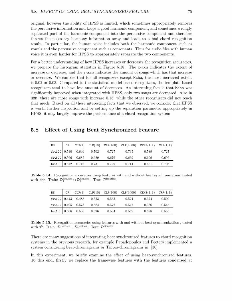
5.8. EFFECT OF USING BEAT SYNCHRONIZED FEATURE 75
original, however the ability of HPSS is limited, which sometimes appropriately removesthe percussive information and keeps a good harmonic component; and sometimes wronglyseparated part of the harmonic component into the percussive component and thereforethrows the necessary harmony information away and leads to a bad chord recognitionresult. In particular, the human voice includes both the harmonic component such asvowels and the percussive component such as consonants. Thus for audio files with humanvoice it is even harder for HPSS to appropriately separate the two components.
For a better understanding of how HPSS increases or decreases the recognition accuracies,we prepare the histogram statistics in Figure 5.18. The x-axis indicates the extent ofincrease or decrease, and the y-axis indicates the amount of songs which has that increaseor decrease. We can see that for all recognizers except Maha, the most increased extentis 0.02 or 0.03. Compared to the statistical model based recognizers, the template basedrecognizers tend to have less amount of decreases. An interesting fact is that Maha wassignificantly improved when integrated with HPSS, only two songs are decreased. Also inHMM, there are more songs with increase 0.15, while the other recognizers did not reachthat much. Based on all these interesting facts that we observed, we consider that HPSSis worth further inspection and by setting up the separation parameter appropriately inHPSS, it may largely improve the performance of a chord recognition system.
5.8 Effect of Using Beat Synchronized Feature
BS CP CLP(1) CLP(10) CLP(100) CLP(1000) CENS(1, 1) CRP(1, 1)
fw 100 0.530 0.646 0.702 0.727 0.735 0.589 0.727
fw 500 0.566 0.685 0.689 0.676 0.669 0.609 0.695
bw 1.0 0.572 0.716 0.731 0.729 0.714 0.621 0.708
Table 5.14. Recognition accuracies using features with and without beat synchronization, testedwith HMM. Train: DBeatles
1∪DBeatles
2.. Test: DBeatles.
BS CP CLP(1) CLP(10) CLP(100) CLP(1000) CENS(1, 1) CRP(1, 1)
fw 100 0.443 0.488 0.523 0.533 0.524 0.324 0.509
fw 500 0.495 0.573 0.584 0.572 0.547 0.386 0.545
bw 1.0 0.506 0.586 0.596 0.584 0.559 0.398 0.555
Table 5.15. Recognition accuracies using features with and without beat synchronization , testedwith Tb. Train: DBeatles
1∪ DBeatles
2.. Test: DBeatles.
There are many suggestions of integrating beat synchronized features to chord recognitionsystems in the previous research, for example Papadopoulos and Peeters implemented asystem considering beat-chromagrams or Tactus-chromagrams in [30].
In this experiment, we briefly examine the effect of using beat-synchronized features.To this end, firstly we replace the framewise features with the features condensed at

76 CHAPTER 5. EXPERIMENTS
beats. Secondly, the chord labels are computed for each of the beat-synchronized features.Thirdly, in order to have make the result comparable to the previous statistics, at theevaluation step we keep the framewise evaluation by resampling the computed chord labelsinto frames. Finally, the framewise comparison between computed labels and ground truthlabels are performed and the recognition accuracies are calculated.
Table 5.14 shows the result tested with recognizer HMM and Table 5.15 shows the resultwith Tb. The rows change the strategy of features in turn. fw 100 indicates that eachfeature is computed using a fixed window with length 100 milliseconds, which is the sameas our previous setting where feature rate is 10 Hz. fw 500 means that the window lengthis set to 500 milliseconds. Usually the duration of a beat is 500 milliseconds as well. bw 1.0means that we take the ground truth beat labels to form the beat windows, and averagingthe framewise features inside each beat window to generate the beat-synchronized features.From the tables we can find that using recognizer Tb, for all the features, fw 500 performsbetter than fw 100, and bw 1.0 gets the best result. However using recognizer HMM, theresults varies with the feature types. For example, CP, CLP(1) and CLP(10) get the bestresult with the beat-synchronized features. But for CLP(1000) and CRP(1, 1), the best resultcome from the features with fixed window length 100. We consider that such unstablebehavior is due to the combination of beat-synchronized features with the post-smoothingeffect of HMM. Averaging the original framewise features inside a beat window can beconsidered as a kind of smoothing as well. In this case, the results might be over smoothedand therefore we observe a decrease in recognition accuracy compared to the result usingframewise features.
5.9 Experiments on Classical Dataset
File ID CP CLP(1) CLP(10) CLP(100) CLP(1000) CISP CENS(1, 1) CRP(1, 1)
BachBWV846Fischer 0.613 0.637 0.657 0.680 0.683 0.602 0.558 0.653
Beet5Bernstein 0.648 0.658 0.679 0.700 0.687 0.564 0.653 0.648
ChopMazurkaSmith 0.761 0.773 0.795 0.788 0.773 0.746 0.596 0.717
SchumannKonz 0.750 0.746 0.766 0.811 0.834 0.814 0.757 0.825
Table 5.16. Recognition accuracies of classical dataset using Tb. Test: D4.
File ID CP CLP(1) CLP(10) CLP(100) CLP(1000) CISP CENS(1, 1) CRP(1, 1)
BachBWV846Fischer 0.508 0.578 0.624 0.646 0.653 0.694 0.596 0.738
Beet5Bernstein 0.572 0.585 0.674 0.729 0.759 0.740 0.700 0.849
ChopMazurkaSmith 0.578 0.728 0.712 0.739 0.775 0.811 0.700 0.808
SchumannKonz 0.556 0.553 0.562 0.652 0.722 0.846 0.776 0.854
Table 5.17. Recognition accuracies of classical dataset using HMM. Train: DBeatles1
. Test: D4.
All the datset we used before are from Beatles Album which is the instance of pop music.

5.9. EXPERIMENTS ON CLASSICAL DATASET 77
In this section, as an additional experiment, we test the chord recognition on the classicaldataset D4.
Table 5.16 shows the recognition accuracies of each of the music piece using recognizer Tb.We find that the chords of all these four classical pieces are recognized for at least 0.613,which can be considered as a good result. Table 5.17 shows the recognition accuraciesusing HMM. By comparison of the two tables, we find that generally Tb gets better resultthan HMM for the feature type CP and CLP. In contrast, for feature CISP, CENS and CRP,HMM gets better result than Tb. This is an interesting phenomenon which needs furtherinspection.
We previously assume that the result of using HMM might not be satisfied. Because theparameters of HMM are trained on the pop music, which may not fit for classical music.However, according to the recognition accuracies of the four pieces, we can consider thatthe model still work for classical music. In particular, for CRP, the result using HMM is muchlarger than using Tb for the first three pieces.

78 CHAPTER 5. EXPERIMENTS

Chapter 6
Summary
In this thesis, we introduced an automatic chord recognition system and performed sys-tematic evaluations at different stages with a focus on the effect of different parametersettings and their interaction. To this end, we first transformed the audio data to sev-eral types of feature representations which captured the harmony-related music content.Then, the feature sequences were passed to the chord recognizer module where severalchord recognition methods existed. In template based methods, we previously defined orlearned a set of feature templates, and performed pattern matching with cosine distancemeasure. In statistical model based methods, we learned multivariate Gaussian models torepresent the chord patterns and then used these models to perform pattern matching inseveral methods such as Mahalanobis distance based method, Gaussian probability basedmethod and HMM based method.
Our main contributions can be summarized as follows. Firstly, we developed a modularchord recognition system with various types of features and several chord recognizers.Secondly, we conducted extensive experiments which examined certain parameter settingsand their impacts on chord recognition accuracies, and we present detailed analysis andconclusions.
By testing chord recognition performance using various types of features we gained insightof the characteristics of each type of features. We found that factors such as logarithmiccompression and smoothing in features had significant impact on recognition accuracies.Instead of 12 dimension, using 24 dimension features also improved the results but suchimprovement varied with feature types and recognizers. In the recognizer side, we foundthat the suitability of chord recognizers and features had large impact on recognition ac-curacies. One needed to consider whether the intensity computation of features such asmagnitude or energy, was appropriate for certain recognizers. In the statistical modelbased recognizers. We found that the main contribution of covariance matrix came fromthe diagonal values. One can disregard the off-diagonal values for convenience of analysisyet keep nearly the same recognition accuracies by scaling the diagonal values. Insteadof using trained covariance matrices, manually set covariance matrices worked effectivelyas well. However one needs to adjust the scale to fit different types of features. Finally,the post-smoothing introduced by HMM brought a large improvement to recognition ac-curacies. A crucial factor which made it work was the emphasizing of the self-transition
79

80 CHAPTER 6. SUMMARY
probability. Furthermore, the performance of HMM depended much on the corporationof covariance matrix and transition matrix. It was very sensitive to the values of theentries of these matrices, and any small difference in value setting might totally destroythe performance.
As future work, one could extend the experiments which we briefly discussed such as usingharmonic-percussive source separation as pre-processing step and using beat synchronizedfeatures instead of framewise features. Furthermore, an insight gained from all theseexperiments is that if we could compute a type of feature which successfully emphasizeharmony-related content of the music audio while suppress the unnecessary noise, eventhe simplest recognizer such as binary template-based method will yields a good result.Usually the complex recognizers with many parameters only slightly improve the recogni-tion and the computation efficiency is far less than simple recognizers such as all templatebased methods. Therefore in the future, it is worth to try to enhance our features. Onepossibility is to integrate more information such as the bass note of the chord and the keyinformation in the features.

Appendix A
Source Code
In this chapter, the headers of selected MATLAB functions created during the writingof this thesis are reproduced. The headers contain information about the name of thedescribed function and its input/output behavior.
General Routine of Chord Recognition
Here we provide the general routine of chord recognition system. Firstly, the audio fileis converted to features. Secondly, the chord labels are computed by one of the chordrecognizers. Thirdly, the ground truth labels are prepared. Finally, the computed andground truth labels are compared to express the recognition accuracy via precision andrecall.
%--------------------------------------------------------------------------------------------------%
%step 1. Load or compute features for the audio file.
% The file name and parameter of features are passed as arguments.
[song_features] = audiofile_to_features(filename,parameterFeature);
%step 2. Compute chord labels by one of the chord recognizers.
% Case 1 corresponds to the template-based method which is introduced in Chapter 3
% The other cases correspond to the statistical model-based methods which is introduced in Chapter 4
switch chord_recognizer
case 1
[computed_chords] = template_based_method(song_features,parameterTemplate);
case 2
[computed_chords] = Mahalanobis_distance_based_method(song_features,parameterMaha);
case 3
[computed_chords] = Gaussian_probability_based_method(song_features,parameterGP);
case 4
[computed_chords] = HMM_based_method(song_features,parameterHMM);
end
%step 3. Prepare the annotated ground truth
annotated_chords = parse_annotation_file(filename,parameterAnno);
%step 4. Evaluate recognition accuracy by comparing the computed and ground truth labels.
The method of evaluation is introduced in Chapter 5.
[precision,recall,f_measure] = evaluate_result(computed_chords,annotated_chords,parameter);
%--------------------------------------------------------------------------------------------------%
81

82 APPENDIX A. SOURCE CODE
Procedure of Training the Chord Models and Transition
There are three parameters in the recognizers which needed to be previous trained: Themean vector and the covariance matrix of a Gaussian model which represents a chordpattern, and the transition matrix which describing the chord transitions. The meanvector can be also considered as the averaged templates of a chord pattern. The functionprocedure training first takes a trainining dataset as input and extract all the featuresand corresponding labels, then compute all these parameters and finally save them in afile.
Sample usage:[chord_models,transition_matrix] = procedure_training(trainDataset);
%--------------------------------------------------------------------------------------------------%
%step 1. extract all the features and corresponding labels from the training dataset
for n=1:size(trainDataset)
filename = strcat(trainDataset{n});
%load or compute features for the audio file
[f_features] = audiofile_to_features(filename,parameterFeature);
%prepare the annotated ground truth
[chord_labels] = parse_annotation_file(filename,parameterAnno);
%Accumulating all features
[all_features]=[all_features,f_features]; % combine features;
%Accumulating all labels
[all_labels] = [all_labels ; chord_labels];
end
%step 2. train the mean vector and covariance matrix for each of the Gaussian model which
% represent the chord pattern. Note that the mean vector can be used as averaged templates.
[chord_models] = train_MeanVectorAndCovMatrix(all_features,all_labels);
%train the transition matrix which save the transition probabilities between chords
[transition_matrix] = train_TransitionMatrix(L_CP);
%step 3. save all these parameters in a file
save_transition_model(transition_matrix);
save_chord_models(chord_models);
%--------------------------------------------------------------------------------------------------%
Feature Extraction
The audiofile to features function is a wrapper to several feature extraction functionsin the Chroma Tool Box [22]. Here we compute a certain type of features, with the typeinformation specified in the parameter.
Sample usage:[f_features] = audiofile_to_features(filename,parameter);
%%%%%%%%%%%%%%%%%%%%%%%%%%%%%%%%%%%%%%%%%%%%%%%%%%%%%%%%%%%%%%%%%%%%%%%%%%%%%%%
% Name: audiofile_to_features
% Date of Revision: 19.01.2011
% Programmer: Nanzhu Jiang
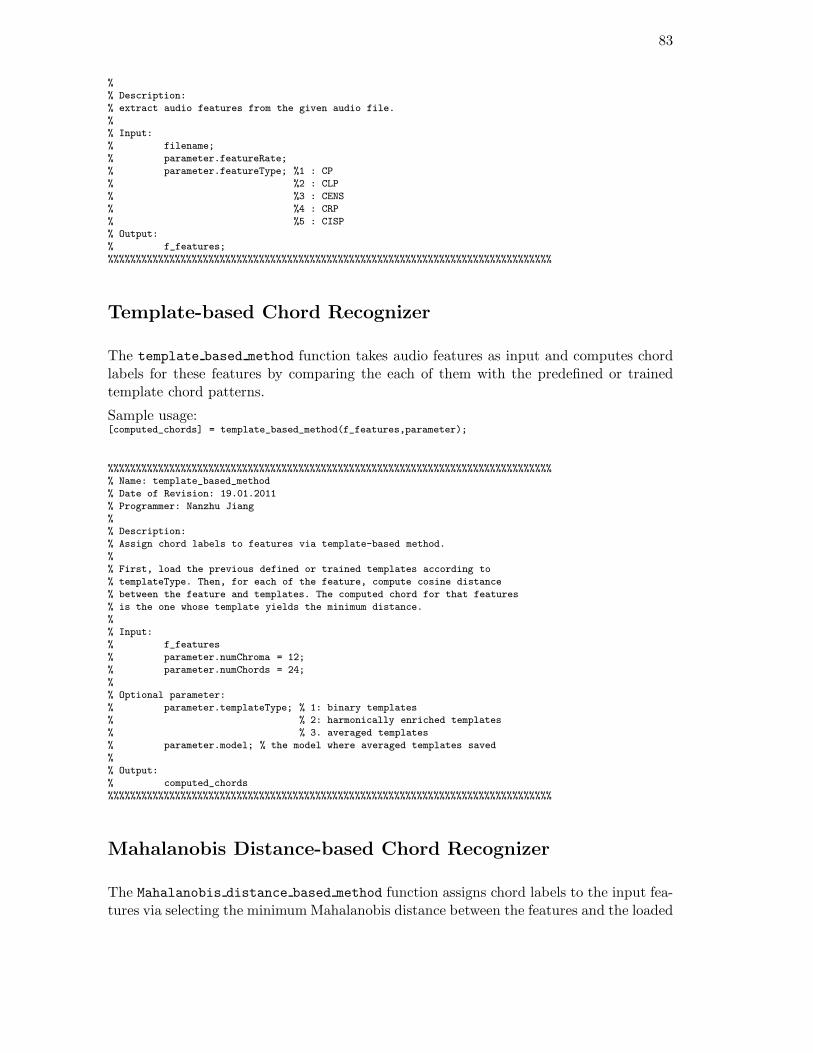
83
%
% Description:
% extract audio features from the given audio file.
%
% Input:
% filename;
% parameter.featureRate;
% parameter.featureType; %1 : CP
% %2 : CLP
% %3 : CENS
% %4 : CRP
% %5 : CISP
% Output:
% f_features;
%%%%%%%%%%%%%%%%%%%%%%%%%%%%%%%%%%%%%%%%%%%%%%%%%%%%%%%%%%%%%%%%%%%%%%%%%%%%%%%
Template-based Chord Recognizer
The template based method function takes audio features as input and computes chordlabels for these features by comparing the each of them with the predefined or trainedtemplate chord patterns.
Sample usage:[computed_chords] = template_based_method(f_features,parameter);
%%%%%%%%%%%%%%%%%%%%%%%%%%%%%%%%%%%%%%%%%%%%%%%%%%%%%%%%%%%%%%%%%%%%%%%%%%%%%%%
% Name: template_based_method
% Date of Revision: 19.01.2011
% Programmer: Nanzhu Jiang
%
% Description:
% Assign chord labels to features via template-based method.
%
% First, load the previous defined or trained templates according to
% templateType. Then, for each of the feature, compute cosine distance
% between the feature and templates. The computed chord for that features
% is the one whose template yields the minimum distance.
%
% Input:
% f_features
% parameter.numChroma = 12;
% parameter.numChords = 24;
%
% Optional parameter:
% parameter.templateType; % 1: binary templates
% % 2: harmonically enriched templates
% % 3. averaged templates
% parameter.model; % the model where averaged templates saved
%
% Output:
% computed_chords
%%%%%%%%%%%%%%%%%%%%%%%%%%%%%%%%%%%%%%%%%%%%%%%%%%%%%%%%%%%%%%%%%%%%%%%%%%%%%%%
Mahalanobis Distance-based Chord Recognizer
The Mahalanobis distance based method function assigns chord labels to the input fea-tures via selecting the minimumMahalanobis distance between the features and the loaded

84 APPENDIX A. SOURCE CODE
chord patterns.
Sample usage:[computed_chords] = Mahalanobis_distance_based_method(f_features,parameter);
%%%%%%%%%%%%%%%%%%%%%%%%%%%%%%%%%%%%%%%%%%%%%%%%%%%%%%%%%%%%%%%%%%%%%%%%%%%%%%%
% Name: Mahalanobis_distance_based_method
% Date of Revision: 19.01.2011
% Programmer: Nanzhu Jiang
%
% Description:
% Assign chord labels to features via Mahalanobis distance-based method.
%
% First, for each of the chord, load the mean vector and covariance matrix
% from the Gaussian model which described the chod pattern. Then, compute the
% Mahalanobis Distance for each of the feature and the chord patterns. The computed
% chord for that features is the one whose pattern yields the minimum distance.
%
% Input:
% f_features;
% parameter.model; %Gaussian models which specify chord patterns
% %For each model, we load the mean vector and the covariance
% matrix which determined the model.
%
% Output:
% computed_chords;
%%%%%%%%%%%%%%%%%%%%%%%%%%%%%%%%%%%%%%%%%%%%%%%%%%%%%%%%%%%%%%%%%%%%%%%%%%%%%%%
Gaussian Probability-based Chord Recognizer
The Gaussian probability based method function represents chord patterns by Gaus-sian models. Here, the Gaussian probability describes the possibility that a feature belongsto a certain chord distribution. The assigned chord for the feature is determined by se-lecting the chord pattern whose model gets the maximum Gaussian probability.
Sample usage:[computed_chords] = Gaussian_probability_based_method(f_features,parameter);
%%%%%%%%%%%%%%%%%%%%%%%%%%%%%%%%%%%%%%%%%%%%%%%%%%%%%%%%%%%%%%%%%%%%%%%%%%%%%%%
% Name: Gaussian_probability_based_method
% Date of Revision: 19.01.2011
% Programmer: Nanzhu Jiang
%
% Description:
% Assign chord labels to features via Gaussian probability-based method.
%
% First, for each of the chord, load the mean vector and covariance matrix
% from the Gaussian model which described the chod pattern. Then, compute the
% Gaussian probability for each of the feature and the chord patterns. The computed
% chord for that features is the one whose pattern yields the maximum probability.
%
% Input:
% f_features;
% parameter.model; %Gaussian models which specify chord patterns
% %For each model, we load the mean vector and the covariance
% matrix which determined the model.
%
% Output:
% computed_chords;
%%%%%%%%%%%%%%%%%%%%%%%%%%%%%%%%%%%%%%%%%%%%%%%%%%%%%%%%%%%%%%%%%%%%%%%%%%%%%%%

85
HMM-based Chord Recognizer
The HMM based method function first computes the Gaussian probabilities for each of thefeature, then treat these probabilities as observation probabilities of the Viterbi algorithm.By plug in the observation and transition probabilities as parameters, the Viterbi algorithmcomputes the chord labels with smoothing of temporal context. The output of Viterbialgorithm is the sequence of final chord labels.
Sample usage:[computed_chords] = HMM_based_method(f_features,parameter);
%%%%%%%%%%%%%%%%%%%%%%%%%%%%%%%%%%%%%%%%%%%%%%%%%%%%%%%%%%%%%%%%%%%%%%%%%%%%%%%
% Name: HMM_based_method
% Date of Revision: 19.01.2011
% Programmer: Nanzhu Jiang
%
% Description:
% Assign chord labels to features via HMM-based method.
%
% Firstly, for each of the chord, load the mean vector and covariance matrix
% from the Gaussian model which described the chod pattern. Load the transition
% matrix which describe the chord transition probabilities.
%
% Secondly, compute the Gaussian probability for each of the feature and the
% chord patterns.
%
% Thirdly, the Gaussian probability is treated as observation probability,
% and the transition matrix is treated transition probability. The chord labels
% are computed via Viterbi algorithm, in which the both probability are plugged in
% as parameter.
%
% Input:
% f_features;
% parameter.model; %Gaussian models which specify chord patterns
% %For each model, we load the mean vector and the covariance
% matrix which determined the model.
%
% parameter.transition_matrix; %24*24 square matrix which saved the transition
% probabilities of the chords.
%
% Output:
% computed_chords;
%%%%%%%%%%%%%%%%%%%%%%%%%%%%%%%%%%%%%%%%%%%%%%%%%%%%%%%%%%%%%%%%%%%%%%%%%%%%%%%
Parse Chord Annotations
The parse annotation file function reads chord annotations from the specified file andmap the original chords to one of the 24 triads. The triad chords are further mapped tointegers for the convenience of the next evaluation step.
Sample usage:[annotated_chords] = parse_annotation_file(filename,parameter);
%%%%%%%%%%%%%%%%%%%%%%%%%%%%%%%%%%%%%%%%%%%%%%%%%%%%%%%%%%%%%%%%%%%%%%%%%%%%%%%
% Name: parse_annotation_file
% Date of Revision: 19.01.2011
% Programmer: Meinard Mueller, Verena Konz, Nanzhu Jiang

86 APPENDIX A. SOURCE CODE
%
% Description:
% parse annotation file, extract chord annotation and segment them into
% frames. The number of annotation frames are equal to the number of
% feature frames specified in the parameter.
%
% Input:
% filename;
% parameter.featureFrames;
% parameter.featureRate;
%
% Output:
% annotated_chords;
%%%%%%%%%%%%%%%%%%%%%%%%%%%%%%%%%%%%%%%%%%%%%%%%%%%%%%%%%%%%%%%%%%%%%%%%%%%%%%%
Result Evaluation
The evaluate result function compare the compare the computed chords with the an-notated chords, and evaluate correctness via precision and recall. The f-measure is takenas the final recognition accuracy.
Sample usage:[precision,recall,f_measure] = evaluate_result(computed_chords,annotated_chords,parameter);
%%%%%%%%%%%%%%%%%%%%%%%%%%%%%%%%%%%%%%%%%%%%%%%%%%%%%%%%%%%%%%%%%%%%%%%%%%%%%%%
% Name: evaluate_result
% Date of Revision: 19.01.2011
% Programmer: Meinard Mueller, Verena Konz, Nanzhu Jiang
%
% Description:
% Result evaluation via precision and recall. Take f-measure as chord recognition
% accuracy.
%
% Input:
% computed_chords;
% annotated_chords;
% parameter;
%
% Optional:
% parameter.neglectNotAnnotatedChords;
%
% Output:
% precision;
% recall;
% f_measure;
%%%%%%%%%%%%%%%%%%%%%%%%%%%%%%%%%%%%%%%%%%%%%%%%%%%%%%%%%%%%%%%%%%%%%%%%%%%%%%%

List of Figures
1.1 C major triad . . . . . . . . . . . . . . . . . . . . . . . . . . . . . . . . . . . . . . . 1
1.2 Three types of chords with different number of notes based on root note C. . . . . 2
1.3 Chromatic circle and pitch perception . . . . . . . . . . . . . . . . . . . . . . . . . 2
1.4 Triads of major, minor, augmented and diminished. . . . . . . . . . . . . . . . . . . 3
1.5 C major triads in root-position and inversions. . . . . . . . . . . . . . . . . . . . . 3
1.6 All 12 major triads. . . . . . . . . . . . . . . . . . . . . . . . . . . . . . . . . . . . 3
1.7 Overview of our chord recognition system. . . . . . . . . . . . . . . . . . . . . . . . 5
1.8 Chord Recognition output visualized by Interpretation Switcher . . . . . . . . . . . 6
1.9 Module of thesis structure. . . . . . . . . . . . . . . . . . . . . . . . . . . . . . . . 8
2.1 A sample array of filters . . . . . . . . . . . . . . . . . . . . . . . . . . . . . . . . . 13
2.2 Pitch features extracted from ChordExample1 . . . . . . . . . . . . . . . . . . . . . 15
2.3 CP features extracted from ChordExample1 . . . . . . . . . . . . . . . . . . . . . . 16
2.4 CPL features extracted from ChordExample1 . . . . . . . . . . . . . . . . . . . . . . 17
2.5 CENS features extracted from ChordExample1 . . . . . . . . . . . . . . . . . . . . . 19
2.6 CRP features extracted from ChordExample1 . . . . . . . . . . . . . . . . . . . . . . 20
2.7 CISP features extracted from ChordExample1 . . . . . . . . . . . . . . . . . . . . . 22
3.1 Binary templates. . . . . . . . . . . . . . . . . . . . . . . . . . . . . . . . . . . . . . 26
3.2 Harmonically enriched templates for C and Cm. . . . . . . . . . . . . . . . . . . . . 28
3.3 Procedure of generating the averaged template T a. . . . . . . . . . . . . . . . . . . 29
3.4 Averaged templates of different features for chord C and Cm. . . . . . . . . . . . . . 31
3.5 Three variation of template sets. . . . . . . . . . . . . . . . . . . . . . . . . . . . . 33
5.1 Bar visualization of Table 5.3. Result comparison from feature side. . . . . . . . . 51
5.2 Comparisons of features. . . . . . . . . . . . . . . . . . . . . . . . . . . . . . . . . . 54
5.3 Visualization of Table 5.5. Effect of logarithmic compression. . . . . . . . . . . . . 55
87

88 LIST OF FIGURES
5.4 Comparisons of different logarithmic compression on chroma features. . . . . . . . 56
5.5 Effect of Smoothing in CENS features. . . . . . . . . . . . . . . . . . . . . . . . . . . 58
5.6 Effect of smoothing in CRP features. . . . . . . . . . . . . . . . . . . . . . . . . . . 58
5.7 Smoothed CENS features on BeatlesLetItBe. . . . . . . . . . . . . . . . . . . . . . 59
5.8 Visualization of Table 5.8. Overall performance of the recognizers. . . . . . . . . . 63
5.9 Error analysis of chord recognizers. . . . . . . . . . . . . . . . . . . . . . . . . . . . 64
5.10 Suppression on off-diagonal values of trained covariance matrix. . . . . . . . . . . . 65
5.11 Scale on diagonal values of trained covariance matrix. . . . . . . . . . . . . . . . . 67
5.12 Scale on diagonal and off-diagonal values of component notes, trained cov. . . . . . 67
5.13 Scale on diagonal and off-diagonal values of component notes, manually set cov. . . 68
5.14 Trained and manually set covariance matrices. . . . . . . . . . . . . . . . . . . . . 68
5.15 Transition Matrix. . . . . . . . . . . . . . . . . . . . . . . . . . . . . . . . . . . . . 69
5.16 Suppression on diagonal values of a transition matrix. . . . . . . . . . . . . . . . . 69
5.17 Histogram of recognition with tuning and without tuning, using recognizer Tb. . . . 71
5.18 Histogram of recognition difference with HPSS, using feature CLP(1000). . . . . . . 74

List of Tables
1.1 Ground truth chord labels of Bach BWV846. . . . . . . . . . . . . . . . . . . . . . 5
3.1 Contributions for the first six harmonics of a note. . . . . . . . . . . . . . . . . . . 28
3.2 Contributions for the first six harmonics of component notes of C . . . . . . . . . . 28
3.3 Mapping function dchord for major and minor triads. . . . . . . . . . . . . . . . . . 30
5.1 Description of the dataset D4. . . . . . . . . . . . . . . . . . . . . . . . . . . . . . 48
5.2 Description of the dataset D20. . . . . . . . . . . . . . . . . . . . . . . . . . . . . . 48
5.3 Overall recognition accuracies. Train: DBeatles1
. Test: DBeatles. . . . . . . . . . . . . 51
5.4 Overall recognition accuracies. Train: DBeatles1 . Test: DBeatles. . . . . . . . . . . . . 52
5.5 Effect of logarithmic compression. . . . . . . . . . . . . . . . . . . . . . . . . . . . . 55
5.6 Effect of pitch range separation. . . . . . . . . . . . . . . . . . . . . . . . . . . . . . 61
5.7 Recognition differences of pitch range separation of CLP. . . . . . . . . . . . . . . . 61
5.8 Recognition differences between recognizers. . . . . . . . . . . . . . . . . . . . . . . 62
5.9 Effect of detuning compensation. . . . . . . . . . . . . . . . . . . . . . . . . . . . . 71
5.10 Recognition accuracies using different training datasets. . . . . . . . . . . . . . . . 73
5.11 Effect of HPSS. . . . . . . . . . . . . . . . . . . . . . . . . . . . . . . . . . . . . . . 73
5.12 Maximum increased recognition difference with and without HPSS. . . . . . . . . 74
5.13 Maximum decreased recognition difference with and without HPSS. . . . . . . . . 74
5.14 Effect of using beat synchronized features test on HMM. . . . . . . . . . . . . . . . . 75
5.15 Effect of using beat synchronized features test on Tb. . . . . . . . . . . . . . . . . . 75
5.16 Chord Recognition of classical dataset using Tb . . . . . . . . . . . . . . . . . . . . 76
5.17 Chord Recognition of classical dataset using HMM . . . . . . . . . . . . . . . . . . . 76
89

90 LIST OF TABLES

Bibliography
[1] AI ACCESS. Multivariate normal distribution, mean vector, covariance and covariancematrix. http://www.aiaccess.net/English/Glossaries/GlosMod/e_gm_multinormal_distri.htm,Retrieved 12.05.2010.
[2] M. A. Bartsch and G. H. Wakefield. Audio thumbnailing of popular music using chroma-basedrepresentations. IEEE Transactions on Multimedia, 7(1):96–104, Feb. 2005.
[3] J. P. Bello and J. Pickens. A robust mid-level representation for harmonic content in music signals. InProceedings of the International Conference on Music Information Retrieval (ISMIR), London, UK,2005.
[4] T. Cho, R. J. Weiss, and J. P. Bello. Exploring common variations in state of the art chord recognitionsystems. Barcelona, Spain, 2010.
[5] Dan Ellis and Jesper Højvang Jensen. Isp tool box. http://kom.aau.dk/project/isound/ , Retrieved31.12.2010.
[6] K. Dressler. Sinusoidal extraction using an efficient implementation of a multi-resolution FFT. Pro-ceedings of 9th International Conference on Digital Audio Effects (DAfX-06), pages 18–20, 2006.
[7] D. P. W. Ellis and G. E. Poliner. Identifying ‘cover songs’ with chroma features and dynamic pro-gramming beat tracking. In Proc. IEEE International Conference on Acoustics, Speech and SignalProcessing (ICASSP), volume 4, Honolulu, Hawaii, USA, Apr. 2007.
[8] R. Gnanadesikan. Methods for statistical Data Analysis of Multivariate Observations. John Wiley &Sons., United States of America, 1977.
[9] E. Gomez. Tonal Description of Music Audio Signals. PhD thesis, UPF Barcelona, 2006.
[10] E. Gomez. Tonal description of polyphonic audio for music content processing. INFORMS Journalon Computing, 18(3):294–304, 2006.
[11] P. Grosche and M. Muller. Extracting predominant local pulse information from music recordings.IEEE Transactions on Audio, Speech, and Language Processing, 2011.
[12] C. Harte and M. Sandler. Automatic chord identification using a quantised chromagram. In Proceed-ings of the Audio Enginerring Society, 2005.
[13] C. Harte, M. Sandler, S. Abdallah, and E. Gomez. Symbolic representation of musical chords: Aproposed syntax for text annotations. In Proceedings of the International Conference on Music In-formation Retrieval (ISMIR), London, GB, 2005.
[14] X. Huang, A. Acero, A. Acero, and H.-W. Hon. Spoken Language Processing: A Guide to Theory,Algorithm, and System Development. Prentice Hall PTR.
[15] A. P. Klapuri, A. J. Eronen, and J. Astola. Analysis of the meter of acoustic musical signals. IEEETransactions on Audio, Speech and Language Processing, 14(1):342–355, 2006.
[16] V. Konz, M. Muller, and S. Ewert. A multi-perspective evaluation framework for chord recognition.In Proceedings of the 11th International Conference on Music Information Retrieval (ISMIR), pages9–14, Utrecht, Netherlands, 2010.
[17] K. Lee. Automatic chord recognition from audio using enhanaced pitch class profile. In Proceedingsof the 7th International Conference on Music Information Retrieval (ISMIR), 2006.
91

92 BIBLIOGRAPHY
[18] B. Logan. Mel frequency cepstral coefficients for music modeling. In Proceedings of the InternationalSymposium on Music Information Retrieval (ISMIR), Plymouth, Massachusetts, 2000.
[19] G. Madazrov and D. Gjorgjevikj. Evaluation of distance measures for multi-class classification inbinary svm decision tree. In Artificial Intelligence and Soft Computing: 10th International Conference(ICAISC), 2010.
[20] J. Makhoul, F. Kubala, R. Schwartz, and R. Weischedel. Performance measures for informationextraction. In In Proceedings of DARPA Broadcast News Workshop, pages 249–252, 1999.
[21] M. Mauch and S. Dixon. Simultaneous estimation of chords and musical context from audio. IEEETrans. Audio, Speech, and Language Processing, 18(6):1280–1289, 2010.
[22] Meinard Muller and Sebastian Ewert and Peter Grosche. Chroma tool box.http://www.mpi-inf.mpg.de/~mmueller/chromatoolbox/, Retrieved 14.12.2010.
[23] M. Muller. Information Retrieval for Music and Motion. Springer Verlag, 2007.
[24] M. Muller and S. Ewert. Towards timbre-invariant audio features for harmony-based music. IEEETransactions on Audio, Speech, and Language Processing (TASLP), 18(3):649–662, 2010.
[25] M. Muller, S. Ewert, and S. Kreuzer. Making chroma features more robust to timbre changes. InProceedings of IEEE International Conference on Acoustics, Speech, and Signal Processing (ICASSP),pages 1869–1872, Taipei, Taiwan, Apr. 2009.
[26] M. Muller, F. Kurth, and M. Clausen. Audio matching via chroma-based statistical features. InProceedings of the 6th International Conference on Music Information Retrieval (ISMIR), pages 288–295, 2005.
[27] N. Ono, K. ichi Miyamoto, H. Kameoka, and S. Sagayama. A real-time equalizer of harmonic andpercussive components in music signals. In Proceedings of the 9th International Conference on MusicInformation Retrieval (ISMIR), Philadelphia, Pennsylvania, USA, 2008.
[28] L. Oudre, Y. Grenier, and C. Fevotte. Template-based chord recognition: Influence of the chordtypes. In Proceedings of the 10th International Conference on Music Information Retrieval (ISMIR),2009.
[29] H. Papadopoulos and G. Peeters. Large-scale study of chord estimation algorithms based on chromarepresentation and hmm. In Proceedings of the International Workshop on Content-based MultimediaIndexing), 2007.
[30] H. Papadopoulos and G. Peeters. Simultaneous estimation of chord progression and downbeats froman audio file. In Proceedings of the IEEE International Conference on Acoustics, Speech and SignalProcessing (ICASSP), pages 121–124, 2008.
[31] L. Rabiner and B.-H. Juang. Fundamentals of Speech Recognition. Prentice Hall Signal ProcessingSeries, 1993.
[32] A. C. Rencher. Methods of Multivariate Analysis. John Wiley & Sons., United States of America,2002.
[33] A. Schafstein. Determining tempo characteristics of expressive music recordings: An algorithmicapproach. Master Thesis, 2009.
[34] G. Taguchi and R. Jugulum. The Mahalanobis-Taguchi Strategy: A Pattern Technology System. JohnWiley & Sons., United States of America, 2002.
[35] Wikipedia. Precision and recall. http://en.wikipedia.org/wiki/Precision_and_recall, Retrieved19.01.2011.
[36] E. Zwicker and H. Fastl. Psychoacoustics, facts and models. Springer Verlag, New York, NY, US,1990.