Embed Size (px)
Citation preview
Analyzing publicly available data: Fitting multilevel models in complex surveys with design
weights, a software based tutorial.
Adam C. Carle, [email protected]
Department of PsychologyUniversity of North Florida
Jacksonville, FL
Office of Research and Sponsored Program’s Research Forum
October 22nd, 2008.
Introduction• How can you get research done at a relatively teaching oriented University?
• Use publicly available data!
• Federal agencies routinely make data available.
• Federal agencies routinely provide grant funds to investigators using the data!
Introduction• Examples:• The Early Childhood Longitudinal Study.
– http://nces.ed.gov/ECLS/index.asp• More generally: http://nces.ed.gov/
• National Survey of Children’s Health:– http://www.cdc.gov/nchs/about/major/slaits/nsch.htm
• More generally: http://www.cdc.gov/nchs/express.htm
• National Epidemiologic Survey on Alcohol and Related Conditions (NESARC)– http://www.nesarc.niaaa.nih.gov/
Introduction• Examples:• National Archive of Criminal Justice Data:
– http://www.icpsr.umich.edu/NACJD/index.html
• Interuniversity Consortium for Political and Social Research:– http://www.icpsr.umich.edu/index.html
• World's largest archive of digital social science data
• Many, many, others!
• International data too!
Introduction• Funding opportunities abound.
• Use SMARTS.
• ORSP can and WILL help you find more!– Dawn OʹConnor.
Introduction• So, what do we do once we get the data?
• Do special analytical problems present?
• What can we do about them?
• Let’s discuss a few “problems” and solutions.
Introduction• As research progressively seeks to understand individual and contextual influences on health, education, families, organizations, analysts will increasingly turn to multilevel models (MLM).
Introduction• Describe which variables predict individual differences.– e.g., Does an individual’s SES status affect their health?
• Uncover which variables predict contextual level differences.– e.g., Does the average amount a state spends on health care affect an individual’s health?
Introduction• Complex survey data provide a rich source of data for these analyses.
– Organize populations into strata or clusters.• e.g., states, counties, or neighborhoods.
– Collect data within the strata or clusters.• e.g., people, schools, families.
Introduction• But these designs violate important statistical assumptions.
– Data no longer independent.
Introduction• MLM explicitly model the clustered nature of survey design.– Good!– More correctly estimate standard errors.– Increase inferential accuracy
• However, MLM may lead to biased estimates when employed in complex survey data. – Caution!– Complex survey designs often include unequal selection probabilities.
Introduction• To address this, in a separate study, I developed a set of current best practice recommendations for handling design weights in MLM.
• UNF has the software capable of doing what I recommend!
• Let me show you!
Introduction• I fit two models representing “typical” MLM models.
• They examine a continuous outcome…– The number of months CSHCN go without insurance.
• as a function of a level‐1 predictor…– “family income”
• and a level‐2 predictor.– “proportion of families in poverty in a state”
Methods• Publicly available data from the 2005‐2006 National Survey of Children with Special Health Care Needs (NS‐CSHCN)– ftp://ftp.cdc.gov/pub/Health_Statistics/NCHS/slaits_cshcn_survey/2005_2006/Datasets/
• Sponsored by the Maternal and Child Health Bureau (MCHB) and conducted by the National Center for Health Statistics (NCHS).
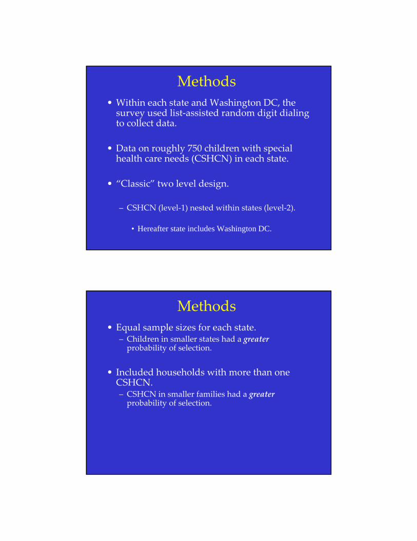
Methods• Within each state and Washington DC, the survey used list‐assisted random digit dialing to collect data.
• Data on roughly 750 children with special health care needs (CSHCN) in each state.
• “Classic” two level design.
– CSHCN (level‐1) nested within states (level‐2).
• Hereafter state includes Washington DC.
Methods• Equal sample sizes for each state.
– Children in smaller states had a greaterprobability of selection.
• Included households with more than one CSHCN.– CSHCN in smaller families had a greaterprobability of selection.
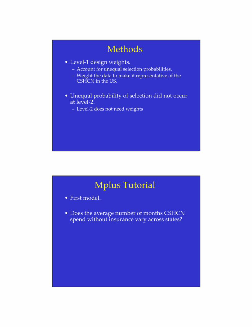
Methods• Level‐1 design weights.
– Account for unequal selection probabilities.– Weight the data to make it representative of the CSHCN in the US.
• Unequal probability of selection did not occur at level‐2. – Level‐2 does not need weights
Mplus Tutorial• First model.
• Does the average number of months CSHCN spend without insurance vary across states?
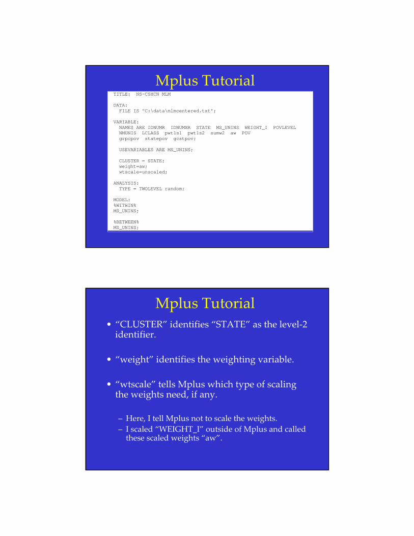
Mplus Tutorial TITLE: NS-CSHCN MLM
DATA: FILE IS "C:\data\mlmcentered.txt";
VARIABLE: NAMES ARE IDNUMR IDNUMXR STATE MS_UNINS WEIGHT_I POVLEVEL NMUNIS LCLASS pwt1s1 pwt1s2 sumw2 aw POV grpcpov statepov gcstpov;
USEVARIABLES ARE MS_UNINS;
CLUSTER = STATE; weight=aw; wtscale=unscaled;
ANALYSIS: TYPE = TWOLEVEL random;
MODEL: %WITHIN% MS_UNINS;
%BETWEEN% MS_UNINS;
Mplus Tutorial• “CLUSTER” identifies “STATE” as the level‐2 identifier.
• “weight” identifies the weighting variable.
• “wtscale” tells Mplus which type of scaling the weights need, if any.
– Here, I tell Mplus not to scale the weights.– I scaled “WEIGHT_I” outside of Mplus and called these scaled weights “aw”.
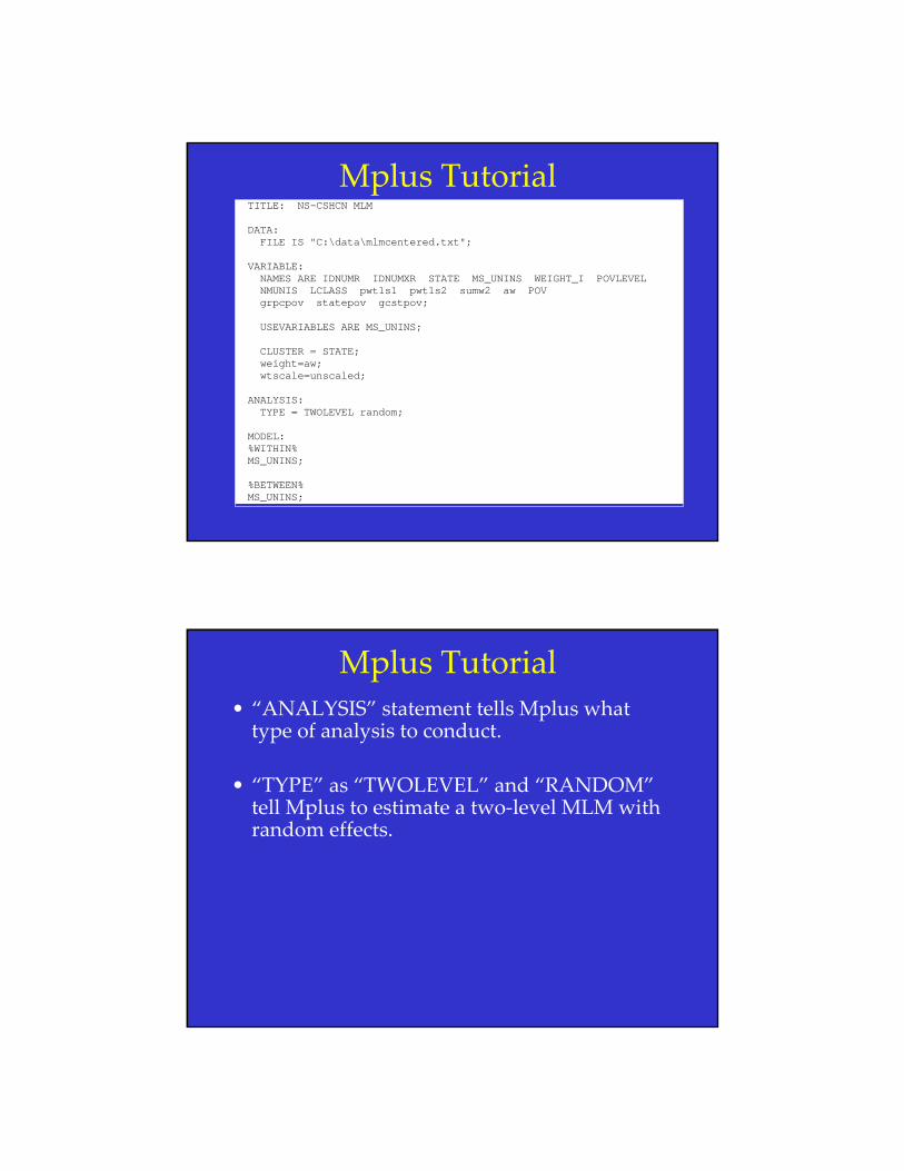
Mplus Tutorial TITLE: NS-CSHCN MLM
DATA: FILE IS "C:\data\mlmcentered.txt";
VARIABLE: NAMES ARE IDNUMR IDNUMXR STATE MS_UNINS WEIGHT_I POVLEVEL NMUNIS LCLASS pwt1s1 pwt1s2 sumw2 aw POV grpcpov statepov gcstpov;
USEVARIABLES ARE MS_UNINS;
CLUSTER = STATE; weight=aw; wtscale=unscaled;
ANALYSIS: TYPE = TWOLEVEL random;
MODEL: %WITHIN% MS_UNINS;
%BETWEEN% MS_UNINS;
Mplus Tutorial• “ANALYSIS” statement tells Mplus what type of analysis to conduct.
• “TYPE” as “TWOLEVEL” and “RANDOM”tell Mplus to estimate a two‐level MLM with random effects.

Mplus Tutorial TITLE: NS-CSHCN MLM
DATA: FILE IS "C:\data\mlmcentered.txt";
VARIABLE: NAMES ARE IDNUMR IDNUMXR STATE MS_UNINS WEIGHT_I POVLEVEL NMUNIS LCLASS pwt1s1 pwt1s2 sumw2 aw POV grpcpov statepov gcstpov;
USEVARIABLES ARE MS_UNINS;
CLUSTER = STATE; weight=aw; wtscale=unscaled;
ANALYSIS: TYPE = TWOLEVEL random;
MODEL: %WITHIN% MS_UNINS;
%BETWEEN% MS_UNINS;
Mplus Tutorial• “%BETWEEN%” specifies the level‐2 part of the model.
• To specify the unconditional model, I included the outcome variable “MS_UNINS” under both the “%WITHIN%” and “%BETWEEN%”statements. – Estimates the MS_UNINS’s intercept (%WITHIN%)– Estimates the variance in MS_UNINS across states (%BETWEEN%).
• Mplus automatically estimates the residual variance.
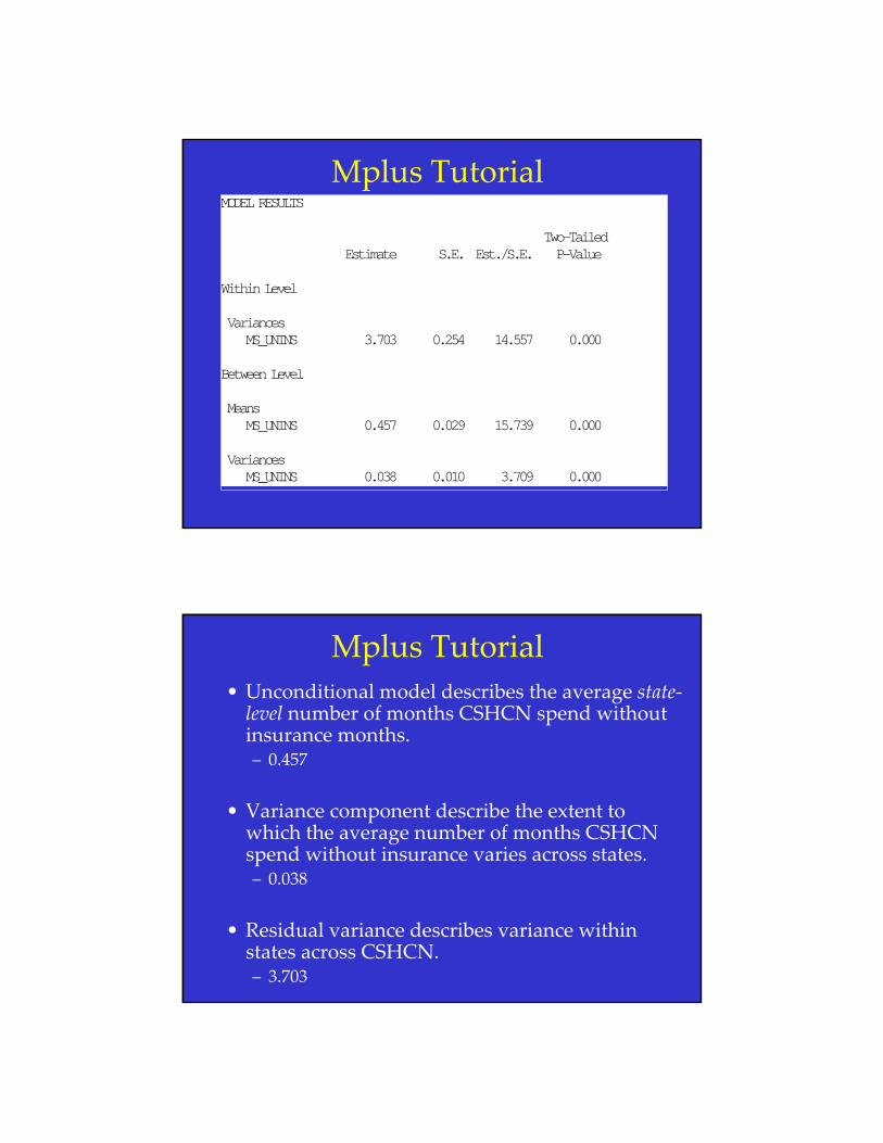
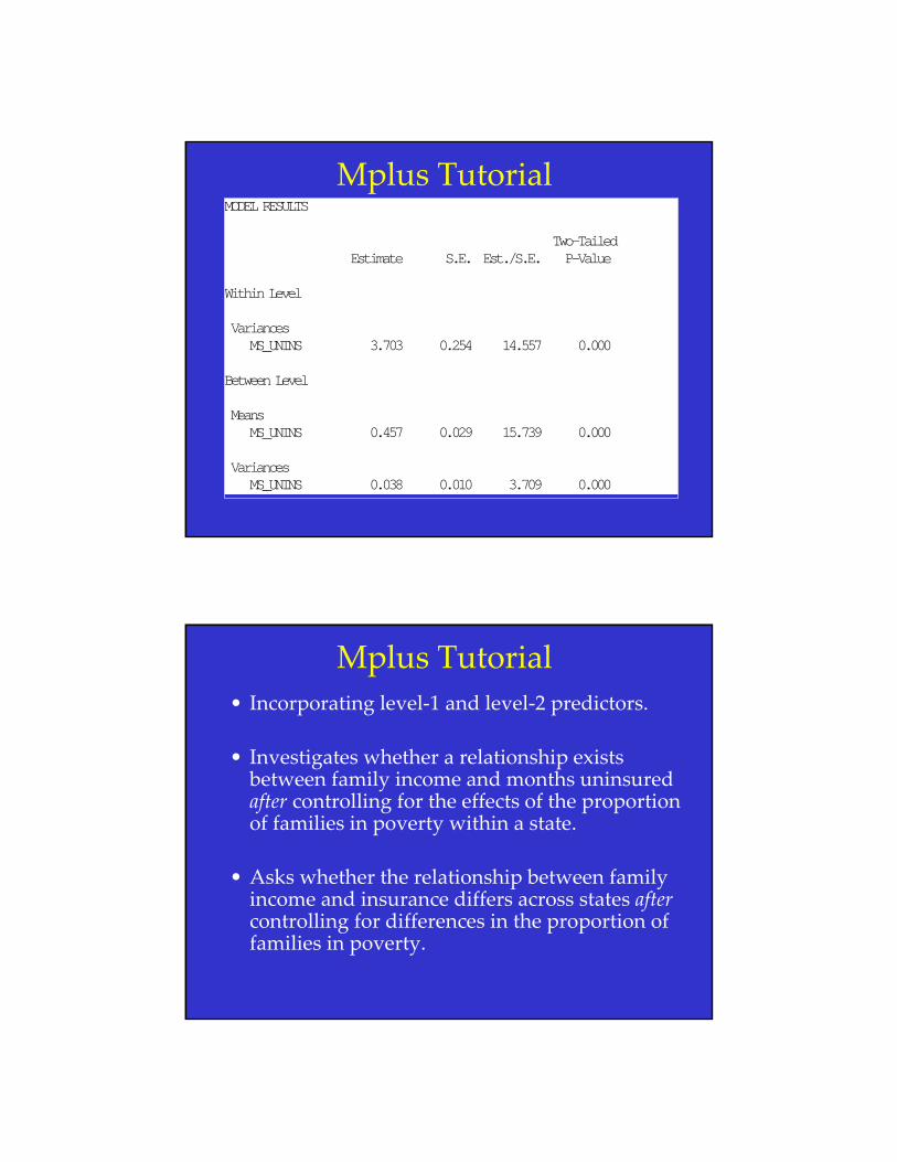
Mplus TutorialMODEL RESULTS
Two-Tailed Estimate S.E. Est./S.E. P-Value
Within Level
Variances MS_UNINS 3.703 0.254 14.557 0.000
Between Level
Means MS_UNINS 0.457 0.029 15.739 0.000
Variances MS_UNINS 0.038 0.010 3.709 0.000
Mplus Tutorial• Unconditional model describes the average state‐level number of months CSHCN spend without insurance months.– 0.457
• Variance component describe the extent to which the average number of months CSHCN spend without insurance varies across states.– 0.038
• Residual variance describes variance within states across CSHCN. – 3.703
Mplus TutorialMODEL RESULTS
Two-Tailed Estimate S.E. Est./S.E. P-Value
Within Level
Variances MS_UNINS 3.703 0.254 14.557 0.000
Between Level
Means MS_UNINS 0.457 0.029 15.739 0.000
Variances MS_UNINS 0.038 0.010 3.709 0.000
Mplus Tutorial• Incorporating level‐1 and level‐2 predictors.
• Investigates whether a relationship exists between family income and months uninsured after controlling for the effects of the proportion of families in poverty within a state.
• Asks whether the relationship between family income and insurance differs across states aftercontrolling for differences in the proportion of families in poverty.
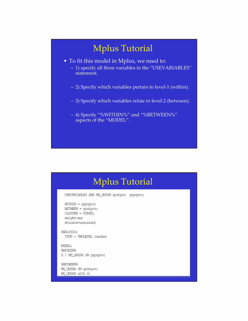
Mplus Tutorial• To fit this model in Mplus, we need to:
– 1) specify all three variables in the “USEVARIABLES”statement.
– 2) Specify which variables pertain to level‐1 (within).
– 3) Specify which variables relate to level‐2 (between).
– 4) Specify “%WITHIN%” and “%BETWEEN%”aspects of the “MODEL”.
Mplus Tutorial USEVARIABLES ARE MS_UNINS gcstpov grpcpov;
WITHIN = grpcpov; BETWEEN = gcstpov; CLUSTER = STATE; weight=aw; wtscale=unscaled;
ANALYSIS: TYPE = TWOLEVEL random;
MODEL: %WITHIN% S | MS_UNINS ON grpcpov;
%BETWEEN% MS_UNINS ON gcstpov; MS_UNINS with S;
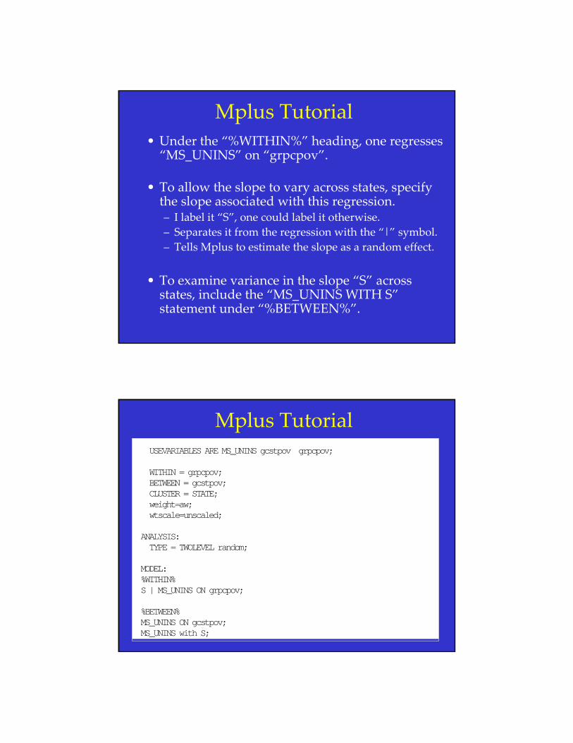
Mplus Tutorial• Under the “%WITHIN%” heading, one regresses “MS_UNINS” on “grpcpov”.
• To allow the slope to vary across states, specify the slope associated with this regression.– I label it “S”, one could label it otherwise.– Separates it from the regression with the “|” symbol. – Tells Mplus to estimate the slope as a random effect.
• To examine variance in the slope “S” across states, include the “MS_UNINS WITH S”statement under “%BETWEEN%”.
Mplus Tutorial USEVARIABLES ARE MS_UNINS gcstpov grpcpov;
WITHIN = grpcpov; BETWEEN = gcstpov; CLUSTER = STATE; weight=aw; wtscale=unscaled;
ANALYSIS: TYPE = TWOLEVEL random;
MODEL: %WITHIN% S | MS_UNINS ON grpcpov;
%BETWEEN% MS_UNINS ON gcstpov; MS_UNINS with S;
Mplus Tutorial• To incorporate the level‐2 predictor, one includes “MS_UNINS ON gcstpov”.
• Reflects the regression of the proportion of families in poverty on months uninsured.– Predicts months uninsured from the proportion of families in poverty.
Mplus Tutorial• All output now reflects conditional statements.
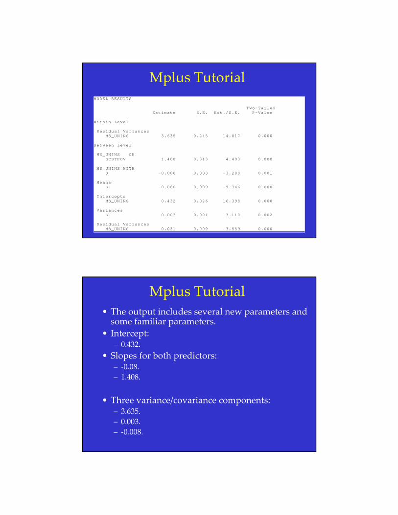
Mplus TutorialMODEL RESULTS
Two-Tailed Estimate S.E. Est./S.E. P-Value
Within Level
Residual Variances MS_UNINS 3.635 0.245 14.817 0.000
Between Level
MS_UNINS ON GCSTPOV 1.408 0.313 4.493 0.000
MS_UNINS WITH S -0.008 0.003 -3.208 0.001
Means S -0.080 0.009 -9.346 0.000
Intercepts MS_UNINS 0.432 0.026 16.398 0.000
Variances S 0.003 0.001 3.118 0.002
Residual Variances MS_UNINS 0.031 0.009 3.559 0.000
Mplus Tutorial• The output includes several new parameters and some familiar parameters.
• Intercept:– 0.432.
• Slopes for both predictors:– ‐0.08.– 1.408.
• Three variance/covariance components:– 3.635.– 0.003.– ‐0.008.
Mplus TutorialMODEL RESULTS
Two-Tailed Estimate S.E. Est./S.E. P-Value
Within Level
Residual Variances MS_UNINS 3.635 0.245 14.817 0.000
Between Level
MS_UNINS ON GCSTPOV 1.408 0.313 4.493 0.000
MS_UNINS WITH S -0.008 0.003 -3.208 0.001
Means S -0.080 0.009 -9.346 0.000
Intercepts MS_UNINS 0.432 0.026 16.398 0.000
Variances S 0.003 0.001 3.118 0.002
Residual Variances MS_UNINS 0.031 0.009 3.559 0.000
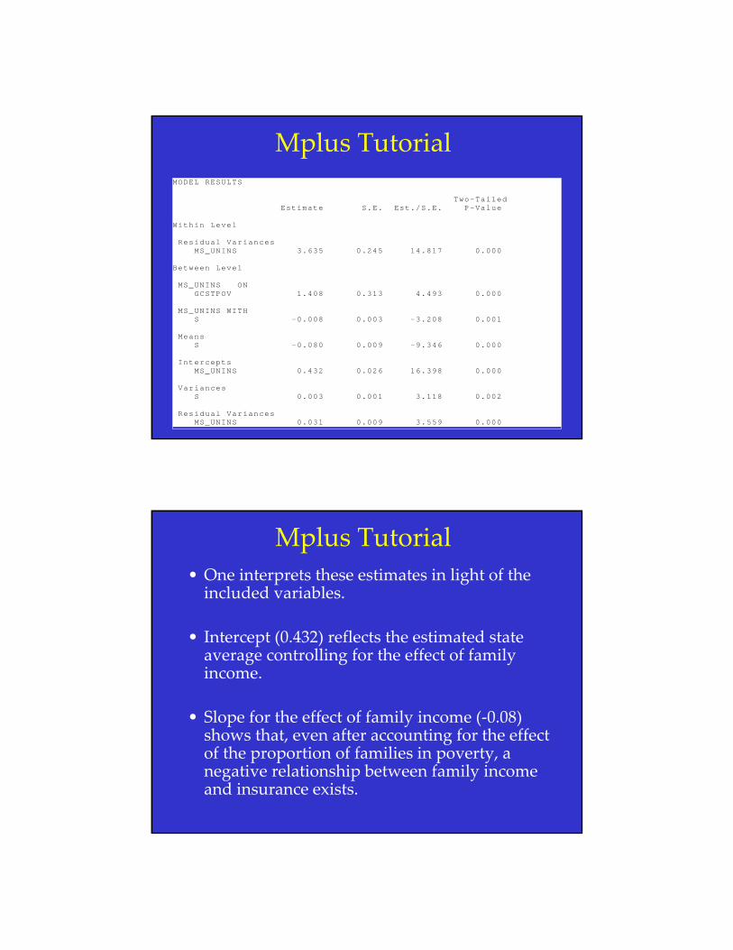
Mplus Tutorial• One interprets these estimates in light of the included variables.
• Intercept (0.432) reflects the estimated state average controlling for the effect of family income.
• Slope for the effect of family income (‐0.08) shows that, even after accounting for the effect of the proportion of families in poverty, a negative relationship between family income and insurance exists.
Mplus TutorialMODEL RESULTS
Two-Tailed Estimate S.E. Est./S.E. P-Value
Within Level
Residual Variances MS_UNINS 3.635 0.245 14.817 0.000
Between Level
MS_UNINS ON GCSTPOV 1.408 0.313 4.493 0.000
MS_UNINS WITH S -0.008 0.003 -3.208 0.001
Means S -0.080 0.009 -9.346 0.000
Intercepts MS_UNINS 0.432 0.026 16.398 0.000
Variances S 0.003 0.001 3.118 0.002
Residual Variances MS_UNINS 0.031 0.009 3.559 0.000
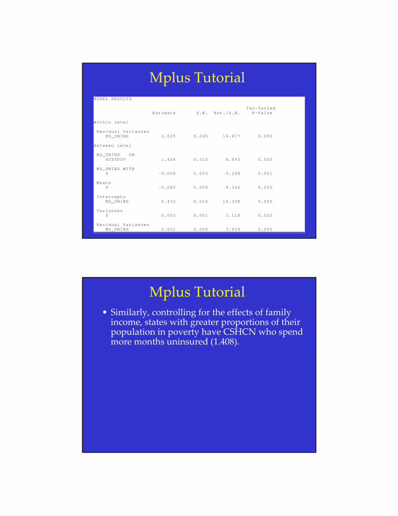
Mplus Tutorial• Similarly, controlling for the effects of family income, states with greater proportions of their population in poverty have CSHCN who spend more months uninsured (1.408).
Mplus TutorialMODEL RESULTS
Two-Tailed Estimate S.E. Est./S.E. P-Value
Within Level
Residual Variances MS_UNINS 3.635 0.245 14.817 0.000
Between Level
MS_UNINS ON GCSTPOV 1.408 0.313 4.493 0.000
MS_UNINS WITH S -0.008 0.003 -3.208 0.001
Means S -0.080 0.009 -9.346 0.000
Intercepts MS_UNINS 0.432 0.026 16.398 0.000
Variances S 0.003 0.001 3.118 0.002
Residual Variances MS_UNINS 0.031 0.009 3.559 0.000
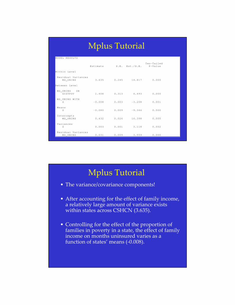
Mplus Tutorial• The variance/covariance components!
• After accounting for the effect of family income, a relatively large amount of variance exists within states across CSHCN (3.635).
• Controlling for the effect of the proportion of families in poverty in a state, the effect of family income on months uninsured varies as a function of states’ means (‐0.008).
Mplus TutorialMODEL RESULTS
Two-Tailed Estimate S.E. Est./S.E. P-Value
Within Level
Residual Variances MS_UNINS 3.635 0.245 14.817 0.000
Between Level
MS_UNINS ON GCSTPOV 1.408 0.313 4.493 0.000
MS_UNINS WITH S -0.008 0.003 -3.208 0.001
Means S -0.080 0.009 -9.346 0.000
Intercepts MS_UNINS 0.432 0.026 16.398 0.000
Variances S 0.003 0.001 3.118 0.002
Residual Variances MS_UNINS 0.031 0.009 3.559 0.000
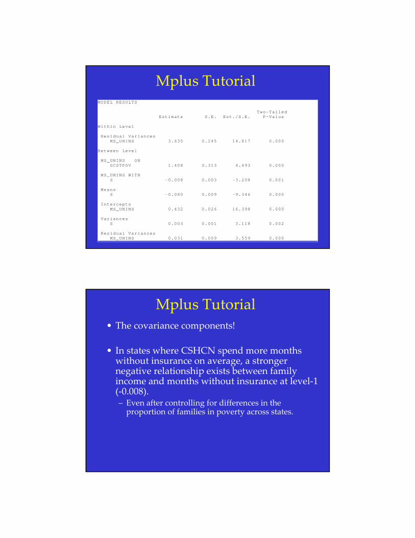
Mplus Tutorial• The covariance components!
• In states where CSHCN spend more months without insurance on average, a stronger negative relationship exists between family income and months without insurance at level‐1 (‐0.008).– Even after controlling for differences in the proportion of families in poverty across states.

Mplus TutorialMODEL RESULTS
Two-Tailed Estimate S.E. Est./S.E. P-Value
Within Level
Residual Variances MS_UNINS 3.635 0.245 14.817 0.000
Between Level
MS_UNINS ON GCSTPOV 1.408 0.313 4.493 0.000
MS_UNINS WITH S -0.008 0.003 -3.208 0.001
Means S -0.080 0.009 -9.346 0.000
Intercepts MS_UNINS 0.432 0.026 16.398 0.000
Variances S 0.003 0.001 3.118 0.002
Residual Variances MS_UNINS 0.031 0.009 3.559 0.000
Mplus Tutorial• Lastly, statistically significant variance exists in the slopes across states even after controlling for effect of family income (0.031).
Mplus Tutorial• Could include numerous other variables.
• And!– Could include cross‐level interactions!
Conclusion• Take home points:
• A vast treasure trove of publicly available data exists.
• This data often needs special statistical analyses.
• Incorrectly analyzing that data will lead to incorrect inferential decisions and faulty research.
• UNF has the software you need to conduct your analyses!
Analyzing publicly available data: Fitting multilevel models in complex surveys with design
weights, a software based tutorial.
Adam C. Carle, [email protected]
Department of PsychologyUniversity of North Florida
Jacksonville, FL
Office of Research and Sponsored Program’s Research Forum
October 22nd, 2008.