Embed Size (px)
Citation preview
Universitat Stuttgart - Institut fur Wasser- undUmweltsystemmodellierung
Lehrstuhl fur Hydromechanik und HydrosystemmodellierungProf. Dr.-Ing. Rainer Helmig
Bachelor Thesis
Analytical Solution for Determining Brine
Leakage Along a Salt Wall
Submitted by
Simon Scholz
Matriculation Number
2714653
Stuttgart, December 9, 2014
Examiners: apl. Prof. Dr.-Ing. Holger Class
PD Dr. rer. nat. Bernd Flemisch, M.Sc
Supervisor: Dipl.-Ing. Alexander Kissinger
I hereby state that this Bachelor thesis has been written independently. I noted all
sources that were used and marked all statements that originate from other authors.
This work, or essential parts of it, is not part of other examination procedures.
Furthermore, I did not publish this work or parts of it. I also assure that the
electronic copy of this work is identical to other copies.
Hiermit versichere ich, dass ich die vorliegende Arbeit selbststandig verfasst habe. Ich
habe keine anderen als die angegebenen Quellen verwendet und alle Aussagen, die
wortlich oder sinngemaß aus anderen Werken ubernommen wurden, als solche
gekennzeichnet. Diese Arbeit, oder wesentliche Teile davon, ist nicht Gegenstand
eines anderen Prufungsverfahrens. Sie ist außerdem von mir weder vollstandig noch
teilweise veroffentlicht worden. Ebenfalls bestatige ich, dass das elektronisch
eingereichte Exemplar mit anderen Exemplaren ubereinstimmt.
Stuttgart, December 9, 2014
Simon Scholz
Contents
1 Motivation 1
1.1 Introduction . . . . . . . . . . . . . . . . . . . . . . . . . . . . . . . . . 1
1.2 Analytical solution . . . . . . . . . . . . . . . . . . . . . . . . . . . . . 2
1.3 Aims . . . . . . . . . . . . . . . . . . . . . . . . . . . . . . . . . . . . . 3
1.4 Structure of this thesis . . . . . . . . . . . . . . . . . . . . . . . . . . . 4
2 Problem Description and Assumptions 5
2.1 Fault structure . . . . . . . . . . . . . . . . . . . . . . . . . . . . . . . 5
2.2 Salt wall structure . . . . . . . . . . . . . . . . . . . . . . . . . . . . . 6
2.3 Assumptions . . . . . . . . . . . . . . . . . . . . . . . . . . . . . . . . . 6
3 Governing Equations and Solution Method 8
3.1 Equation System . . . . . . . . . . . . . . . . . . . . . . . . . . . . . . 8
3.1.1 Darcy’s Law . . . . . . . . . . . . . . . . . . . . . . . . . . . . . 9
3.1.2 Diffusion equation . . . . . . . . . . . . . . . . . . . . . . . . . 10
3.1.3 Governing equations . . . . . . . . . . . . . . . . . . . . . . . . 10
3.2 Fourier and Laplace transform and inversion . . . . . . . . . . . . . . . 13
3.2.1 Fourier and Laplace transform . . . . . . . . . . . . . . . . . . . 13
3.2.2 Fourier and Laplace inversion . . . . . . . . . . . . . . . . . . . 13
4 Scenarios 15
4.1 Zeidouni two-layer analytical model . . . . . . . . . . . . . . . . . . . . 15
4.1.1 Boundary conditions . . . . . . . . . . . . . . . . . . . . . . . . 16
4.1.2 Leakage rate to the upper aquifer for different values of αu . . . 16
4.1.3 Pressure change in the aquifers . . . . . . . . . . . . . . . . . . 18
4.1.4 Leakage rate comparison to numerical model . . . . . . . . . . . 20
4.2 Multiple layer analytical model . . . . . . . . . . . . . . . . . . . . . . 23
4.2.1 Boundary conditions . . . . . . . . . . . . . . . . . . . . . . . . 23
4.2.2 Leakage rate comparison for multi-layer or two-layer systems . . 25
4.3 North German Basin multiple layer analytical model . . . . . . . . . . 26
4.3.1 Boundary conditions . . . . . . . . . . . . . . . . . . . . . . . . 27
4.3.2 Choice of confining layers . . . . . . . . . . . . . . . . . . . . . 27
4.3.3 Leakage rate comparison . . . . . . . . . . . . . . . . . . . . . . 29
I
CONTENTS II
4.4 Limitations . . . . . . . . . . . . . . . . . . . . . . . . . . . . . . . . . 30
5 Summary 31
6 Outlook 33
List of Figures
1.1 Schematic of a typical fault system with a fault core, damage zones and
injection well . . . . . . . . . . . . . . . . . . . . . . . . . . . . . . . . 3
2.1 Fault components in rock . . . . . . . . . . . . . . . . . . . . . . . . . . 6
2.2 Idealized two-layer fault system with boundary conditions modified after
Zeidouni [20] showing a single injection well and the fault zone. . . . . 7
3.1 Schematic overview of the solution method to model leakage through a
fault zone for a two-layer system. . . . . . . . . . . . . . . . . . . . . . 9
4.1 Idealized two-layer fault system with boundary conditions modified after
Zeidouni [20] showing a single injection well and the fault zone. . . . . 15
4.2 Dimensionless leakage rate qlD using different values for αu, considering
zero pressure change in the upper aquifer . . . . . . . . . . . . . . . . . 17
4.3 Pressure changes in the injection aquifer . . . . . . . . . . . . . . . . . 19
4.4 Pressure changes in the upper aquifer . . . . . . . . . . . . . . . . . . . 20
4.5 Dimensionless leakage rate qlD comparison to numerical model for the
two-layer . . . . . . . . . . . . . . . . . . . . . . . . . . . . . . . . . . . 22
4.6 Dimensionless leakage rate qlD for numerical two-layer model . . . . . . 23
4.7 Idealized multi-layer fault system with boundary conditions modified
after Zeidouni [20] showing a single injection well and the fault zone
intersecting all aquifers. . . . . . . . . . . . . . . . . . . . . . . . . . . 24
4.8 Dimensionless leakage to upper aquifers 1, 8 and 15 . . . . . . . . . . . 25
4.9 Idealized North German Basin multi-layer fault system with boundary
conditions. . . . . . . . . . . . . . . . . . . . . . . . . . . . . . . . . . . 27
4.10 Leakage to upper aquifers - North German Basin multi-layer . . . . . . 28
4.11 Dimensionless leakage rate to upper aquifers of North German Basin
with DuMuX comparison . . . . . . . . . . . . . . . . . . . . . . . . . . 30
III
List of Tables
4.1 Input parameters for the two-layer analytical model. . . . . . . . . . . 16
4.2 Input parameters for the two-layer analytical model compared to the
numerical model. . . . . . . . . . . . . . . . . . . . . . . . . . . . . . . 21
4.3 Input parameters for the multi-layer analytical model. . . . . . . . . . . 24
4.4 Layer properties for the North German Basin multiple layer analytical
model. . . . . . . . . . . . . . . . . . . . . . . . . . . . . . . . . . . . 28
IV
Nomenclature
Subscript “D” stands for a dimensionless term
Subscript “f” stands for fault properties
Subscript “u” stands for upper aquifer
Subscripts “1” (with injection) or “2” (without injection) stand for regions separated
by the fault
α dimensionless transmissibility [-]
δ dirac delta function [-]
η diffusivity coefficient [m2
s]
κ intrinsic permeability [m2]
µ viscosity [Pa·s]
ρ density [ kgm3 ]
φ porosity [-]
a well to fault distance [m]
ct total compressibilty [ 1Pa
]
h aquifer thickness [m]
k aquifer permeability [m2]
L leakage pathway [m]
N number of overlying aquifers [-]
P pressure [Pa]
q injection rate [m3
s]
Q volumetric sink/source term [m3
s]
t time [s]
TD dimensionless transmissivity [-]
V
LIST OF TABLES VI
wf fault width [m]
x, y spatial coordinates [m]
FFT Fast Fourier Transform function in MATLAB [-]
Chapter 1
Motivation
1.1 Introduction
Despite all plans and technologies to reduce the energy demand of modern day society,
the industrialization and the immense population growth world wide still have a large
effect on the climate. According to the Third Assessment Report by the International
Panel on Climate Change (IPCC), “human influences are expected to continue to
change atmospheric composition throughout the 21st century” [6]. To match the
demands of modern day society, the use of the subsurface is more popular than ever.
Considering efforts by various governments and organizations to use subsurface sites
for carbon dioxide storage projects, gas storage, waste-water disposal, enhanced oil
recovery or fracking, it has become more relevant to model and monitor possible
geological formations and sites [8].
Especially geologic sites for sequestration of carbon dioxide have been discussed in
the last 10 to 20 years. Most of the considered geologic sequestration sites are either
depleted hydrocarbon reservoirs, brine-bearing saline formations or unmineable coal
seams [16]. If there is a leaky fault, an abandoned well or any other potential pathway
for leakage nearby a subsurface fluid injection or disposal project, the potential of
contaminating possible underground sources of drinking water or other sensitive
aquifers needs to be taken into account. Oldenburg et al. [11] define migration of
brine or CO2 out of a defined storage region as leakage. In our context leakage is only
possible through faults or wells.
Salt formations, such as salt walls and diapirs are an important part of common
rock formations around the world, especially in the North German Basin. Due to
their structure and the disturbed sediments surrounding them, they may be potential
pathways for displaced brine or trace metals from deep aquifers similar to a regular
fault zone.
Salt wall flanks often intersect multiple geological formations and create faulted and
disturbed sediments surrounding them. In the North German Basin, many intrusive
salt walls that deform sediments of upper formations can be found. The permeability
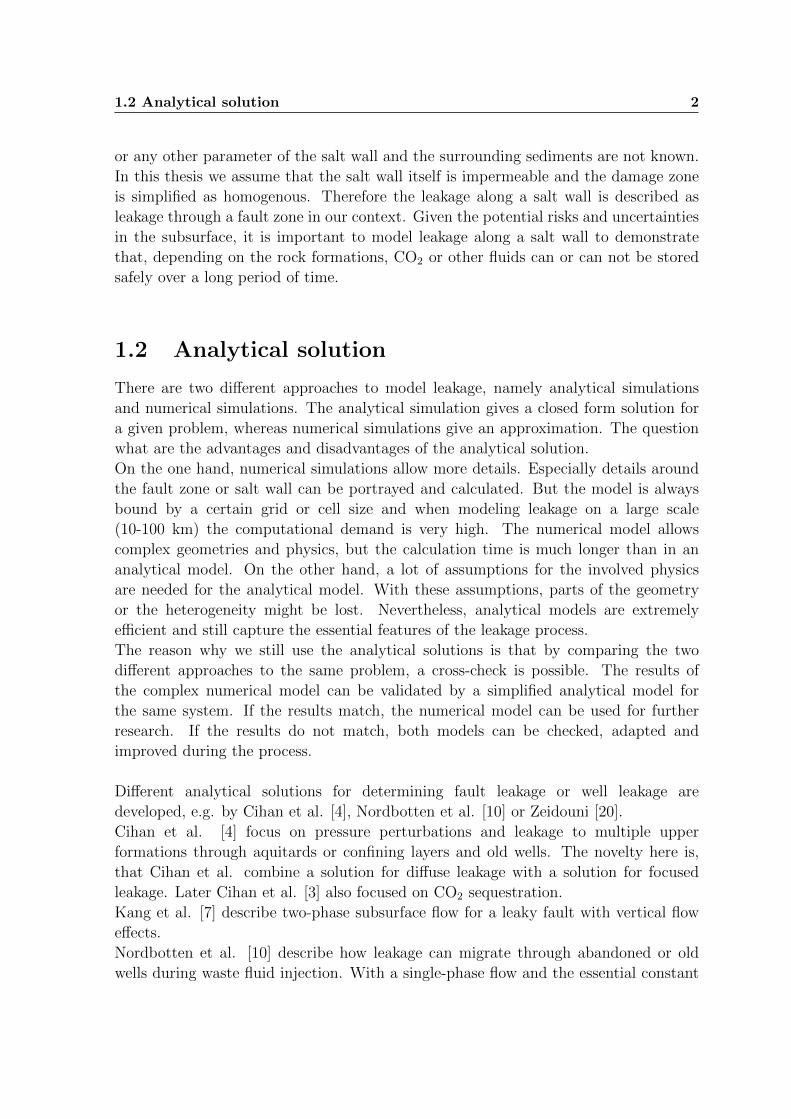
1.2 Analytical solution 2
or any other parameter of the salt wall and the surrounding sediments are not known.
In this thesis we assume that the salt wall itself is impermeable and the damage zone
is simplified as homogenous. Therefore the leakage along a salt wall is described as
leakage through a fault zone in our context. Given the potential risks and uncertainties
in the subsurface, it is important to model leakage along a salt wall to demonstrate
that, depending on the rock formations, CO2 or other fluids can or can not be stored
safely over a long period of time.
1.2 Analytical solution
There are two different approaches to model leakage, namely analytical simulations
and numerical simulations. The analytical simulation gives a closed form solution for
a given problem, whereas numerical simulations give an approximation. The question
what are the advantages and disadvantages of the analytical solution.
On the one hand, numerical simulations allow more details. Especially details around
the fault zone or salt wall can be portrayed and calculated. But the model is always
bound by a certain grid or cell size and when modeling leakage on a large scale
(10-100 km) the computational demand is very high. The numerical model allows
complex geometries and physics, but the calculation time is much longer than in an
analytical model. On the other hand, a lot of assumptions for the involved physics
are needed for the analytical model. With these assumptions, parts of the geometry
or the heterogeneity might be lost. Nevertheless, analytical models are extremely
efficient and still capture the essential features of the leakage process.
The reason why we still use the analytical solutions is that by comparing the two
different approaches to the same problem, a cross-check is possible. The results of
the complex numerical model can be validated by a simplified analytical model for
the same system. If the results match, the numerical model can be used for further
research. If the results do not match, both models can be checked, adapted and
improved during the process.
Different analytical solutions for determining fault leakage or well leakage are
developed, e.g. by Cihan et al. [4], Nordbotten et al. [10] or Zeidouni [20].
Cihan et al. [4] focus on pressure perturbations and leakage to multiple upper
formations through aquitards or confining layers and old wells. The novelty here is,
that Cihan et al. combine a solution for diffuse leakage with a solution for focused
leakage. Later Cihan et al. [3] also focused on CO2 sequestration.
Kang et al. [7] describe two-phase subsurface flow for a leaky fault with vertical flow
effects.
Nordbotten et al. [10] describe how leakage can migrate through abandoned or old
wells during waste fluid injection. With a single-phase flow and the essential constant
1.3 Aims 3
properties they use the superposition principle to investigate the effect of multiple
leakage pathways.
Zeidouni [20] developed a solution for fault leakage involving multiple overlying
formations. He uses existing analytical solutions to verify his results and gives
potential applications for his analytical model. We will focus on the analytical model
developed by Zeidouni, because of his implementation of the fault zone and the
multiple overlying formations. He also provided his MATLAB code, so that the results
can be reproduced easily.
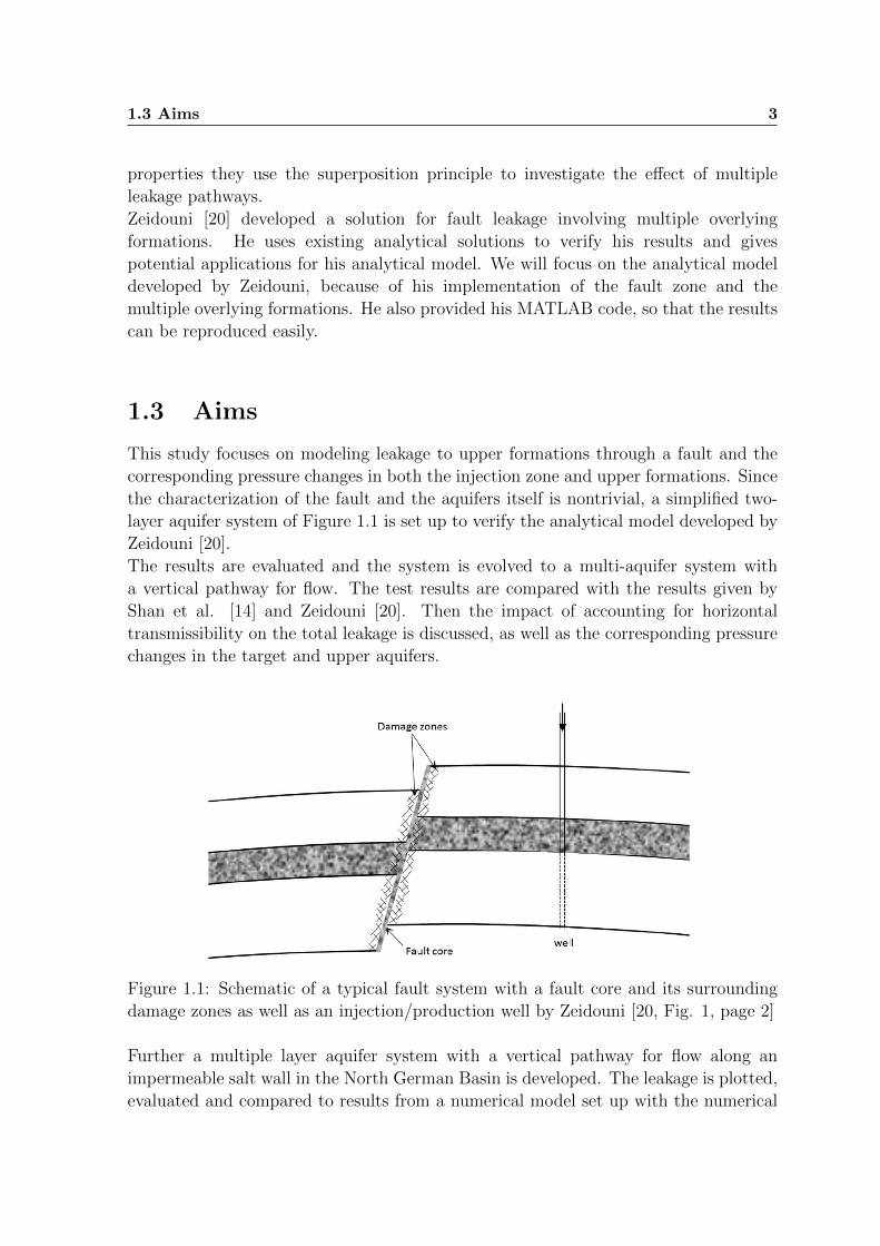
1.3 Aims
This study focuses on modeling leakage to upper formations through a fault and the
corresponding pressure changes in both the injection zone and upper formations. Since
the characterization of the fault and the aquifers itself is nontrivial, a simplified two-
layer aquifer system of Figure 1.1 is set up to verify the analytical model developed by
Zeidouni [20].
The results are evaluated and the system is evolved to a multi-aquifer system with
a vertical pathway for flow. The test results are compared with the results given by
Shan et al. [14] and Zeidouni [20]. Then the impact of accounting for horizontal
transmissibility on the total leakage is discussed, as well as the corresponding pressure
changes in the target and upper aquifers.
Figure 1.1: Schematic of a typical fault system with a fault core and its surrounding
damage zones as well as an injection/production well by Zeidouni [20, Fig. 1, page 2]
Further a multiple layer aquifer system with a vertical pathway for flow along an
impermeable salt wall in the North German Basin is developed. The leakage is plotted,
evaluated and compared to results from a numerical model set up with the numerical
1.4 Structure of this thesis 4
simulator DuMuX [5]. Salt walls are considered because they are an important part
of the geological composition in the North German Basin and are subject of research
in terms of migration to upper aquifers. Salinity of the fluids and transport processes
could be investigated as well, but are not subject of this thesis.
1.4 Structure of this thesis
Chapter 2 describes the problem in general and explains all necessary assumptions.
The aim of Chapter 3 is to provide fundamental knowledge of the problem as well as a
description of the system setup. Then the basic mathematical equations and methods
are given in Section 3.1. The different scenarios with their corresponding parameters
are discussed in Section 4.1 and 4.2, and the results are compared to our reference
models (by Zeidouni [20] and Shan et al. [14]).
Finally the model is adapted to determine brine leakage along a salt wall in the
North German Basin. Therefore, the model is adapted and the results compared to
numerical simulations run in DuMuX in Chapter 4.3.
Chapter 2
Problem Description and
Assumptions
The simplifications used in this thesis are explained here. Most of the system
properties are described in Chapter 3. We take a look at an injection scenario with
one injection well. Fluid is injected into a deep aquifer. It is assumed there is only
one vertical, linear and impermeable fault [20] intersecting all overlying aquifers in
the system without other perturbations or abandoned wells. The aquifers themselves
are assumed to be homogenous and isotropic. Between each aquifer a confining layer,
that does not allow leakage, is set up so that the aquifers are separated and the fault
is the only connection between the aquifers.
2.1 Fault structure
The fault structure is non-trivial and difficult to model in detail due to the different
components of the fault. Caine et al. [2] and others describe faults as a conduit, barrier
or a combination of both.
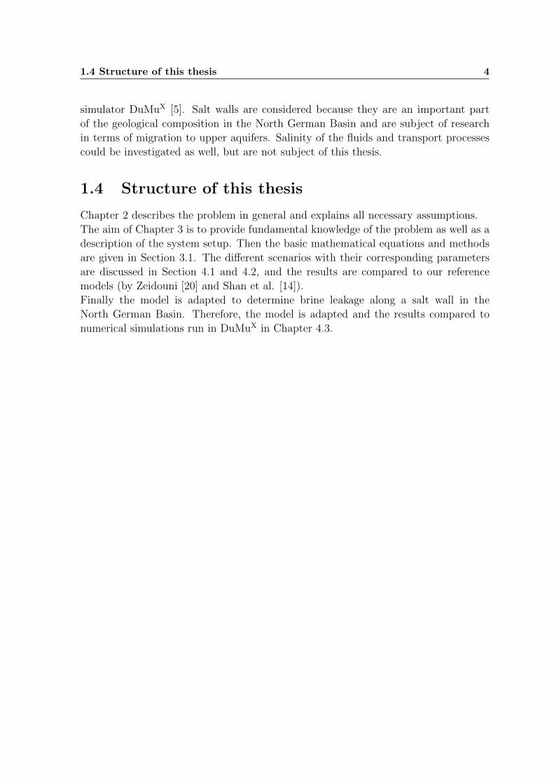
Faults generally have a fault core which is surrounded by damage zones, as we can see
in Fig. 2.1. The fault core often consists of a clay-rich, soft and low permeability gouge
zone called fault gouge [20]. Further, there is fault zone breccia, which may be highly
permeable according to Shan et al. [14] and is broken and sheared fault material [12].
With Zeidouni’s analytical model we do not focus on a detailed fault structure, but
simplify geometry and properties to roughly describe the flow through the fault. Zei-
douni [20] assumes that horizontal resistance of the fault does not have an impact on
the leakage. In Appendix A of his paper Zeidouni demonstrates that lateral transmis-
sibility α and the ratio of upperzone thickness to that of the injection zone hD do not
have an effect when the arithmetic mean of the pressure change at the fault plane is
calculated [20, Paragraph 23]. We will discuss later whether these assumptions are
valid or not.
2.2 Salt wall structure 6
Figure 2.1: Fault components in rock formations by Caine et al., 1996 [2] taken from
http://crustal.usgs.gov/projects/rgb/faults_gw.html [18].
2.2 Salt wall structure
Salt walls and salt domes are common rock formations around the world. Usually
they start growing from relatively small anomalies and can be intrusive (always in
the subsurface) or extrusive (reach the surface). Intrusive salt domes often buckle the
formations above them, whereas extrusive salt domes do not deform upper formations
as much. Each salt wall is unique, and no detailed information on salt walls can be
found. We assume, that they consist of an impermeable salt core and a homogenous
and permeable surrounding transition zones. These zones are assumed to be connected
across all intersecting geological layers for our test cases. Therefore, we describe salt
walls as fault zones and use Zeidouni’s model for fault leakage to model leakage along
a salt wall.
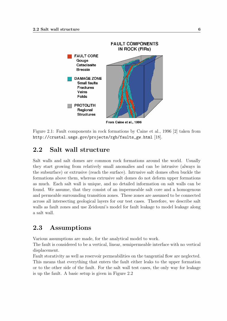
2.3 Assumptions
Various assumptions are made, for the analytical model to work.
The fault is considered to be a vertical, linear, semipermeable interface with no vertical
displacement.
Fault storativity as well as reservoir permeabilities on the tangential flow are neglected.
This means that everything that enters the fault either leaks to the upper formation
or to the other side of the fault. For the salt wall test cases, the only way for leakage
is up the fault. A basic setup is given in Figure 2.2
2.3 Assumptions 7
wf
no-flow boundary
∆P2(x,±∞,t
)=
∆P2(±∞,y,t
)=
0
q
x = 0 x = a
region 2 region 1
k
ku
L
upper zone
injection zone
confining layer
h
hu
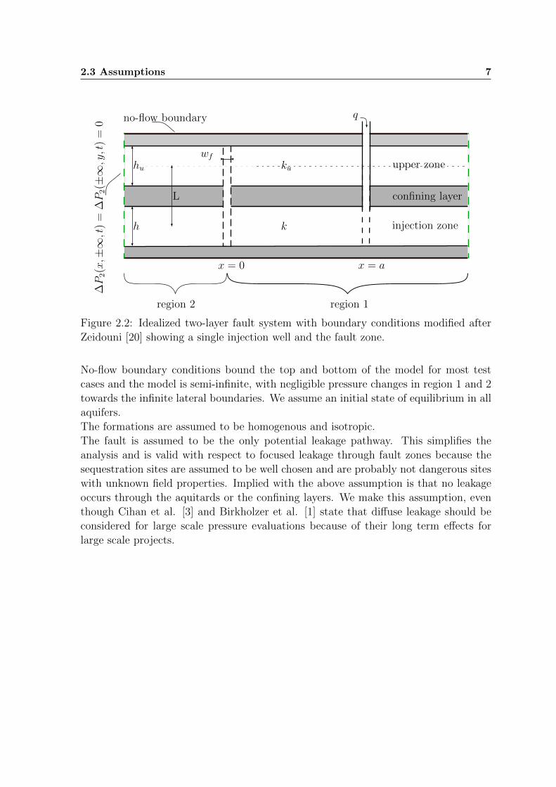
Figure 2.2: Idealized two-layer fault system with boundary conditions modified after
Zeidouni [20] showing a single injection well and the fault zone.
No-flow boundary conditions bound the top and bottom of the model for most test
cases and the model is semi-infinite, with negligible pressure changes in region 1 and 2
towards the infinite lateral boundaries. We assume an initial state of equilibrium in all
aquifers.
The formations are assumed to be homogenous and isotropic.
The fault is assumed to be the only potential leakage pathway. This simplifies the
analysis and is valid with respect to focused leakage through fault zones because the
sequestration sites are assumed to be well chosen and are probably not dangerous sites
with unknown field properties. Implied with the above assumption is that no leakage
occurs through the aquitards or the confining layers. We make this assumption, even
though Cihan et al. [3] and Birkholzer et al. [1] state that diffuse leakage should be
considered for large scale pressure evaluations because of their long term effects for
large scale projects.
Chapter 3
Governing Equations and Solution
Method
In this Chapter, the equations for the model described in Chapter 2 are explained. Us-
ing the code obtained from Zeidouni [20], we model leakage through a fault to multiple
overlying formations. The system setup is based on Zeidouni [20] and Shan et al. [14].
The model is an idealization of the complex system shown in Figure 1.1. They both
assume that different aquifers are separated by aquitards or confining layers that do
not allow flow. The aquifers are assumed to be homogenous and isotropic and are
intersected by a single fault.
For the derivation of the governing equations and the solution method we take a look at
two aquifers with one confining layer in between. The system has a no-flow boundary
condition at the top and the bottom, as well as negligible pressure changes towards
the infinite lateral boundaries. There is a single fault splitting the system in regions 1
(with injection) and 2 (without injection). The Cartesian coordinate is set in a way
that x = 0 at the fault. The injection is at a constant flow rate and no other faults or
old wells are considered.
A detailed description of the general assumptions is given in Chapter 2.3. The pa-
rameters and input data for each test case are given in the corresponding sections of
Chapter 4.
3.1 Equation System
In this thesis an analytical solution for single-phase flow is applied to a hypothetical
two-layer system. In Section 4.2 the system is evolved to a hypothetical multi-layer
system and finally a real multi-layer system is modeled. Because we are only interested
in brine leakage and do not consider local two-phase flow, variable density can be
neglected here [3]. Leakage and pressure buildup in the far field for CO2 storage can
then be reasonably described by a single-phase flow model according to Nicot [9].
3.1 Equation System 9
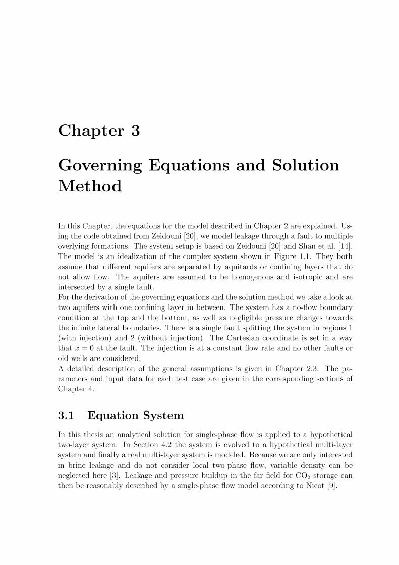
The solution is based on the diffusion equation and Figure 3.1 gives an overview of the
solution method. First of all new dimensionless terms are introduced. Then the set of
partial differential equations is Laplace transformed in the time domain and Fourier
transformed in the space domain. Combining all the equations, we get a system
of coupled ordinary differential equations. This is evaluated in the Laplace-Fourier
domain and then retransformed to calculate the leakage either using the pressure
changes or the derivatives of the pressure changes.
Figure 3.1: Schematic overview of the solution method to model leakage through a
fault zone for a two-layer system.
3.1.1 Darcy’s Law
Darcy’s law is a relationship that was determined experimentally by Henry Darcy.
It provides an accurate description for the ability of a fluid to flow through porous
media. In a simple discrete form it shows that the flux q is a function of the intrinsic
permeability κ and the pressure gradient ∇p divided by the fluid viscosity µ
q = −κµ∇p . (3.1)
3.1 Equation System 10
3.1.2 Diffusion equation
Diffusion is a fundamental transport process in engineering science, especially in envi-
ronmental fluid mechanics. With the mass balance defined as
∇ · (ρ q) + ρQ =∂(ρ φ)
∂t, (3.2)
q can be substituted with Equation 3.1. With the Dupuit assumption for an isotropic
and homogenous aquifer, as well as constant density ρ we get the diffusion equation
∂2∆P
∂x2+∂2∆P
∂y2+����>
Dupuit assumption∂2∆P
∂z2+Q =
φµ ctk
∂∆P
∂t. (3.3)
The diffusivity coefficient η is defined as
η =k
φµ ct, (3.4)
for further simplifications with φ being porosity, µ fluid viscosity and ct total compress-
ibility.
3.1.3 Governing equations
This Section is an explanation of the equations used in this thesis to model flow through
the fault zone and the corresponding pressure perturbations. We follow Zeidouni here.
A more detailed explanation can be found in Appendix A of his paper [20].
Equation 3.3 is used in a special form, with the Dirac delta function to add a point
source term, is used here for region 1 of the injection zone (as previously defined in
Fig. 2.2) to get∂2∆P1
∂x2+∂2∆P1
∂y2+qµ
khδ(x− a)δ(y) =
1
η
∂∆P1
∂t(3.5)
and respectively
∂2∆P2
∂x2+∂2∆P2
∂y2=
1
η
∂∆P2
∂t(3.6)
for region 2, where ∆P1 and ∆P2 stand for pressure changes in the corresponding re-
gion.
q is the volumetric injection rate, µ fluid viscosity, k injection zone permeability, h in-
jection zone thickness, δ the Dirac delta function and a the distance from the injection
well to the fault.
The upper zone equations are similar to Equation 3.6.
3.1 Equation System 11
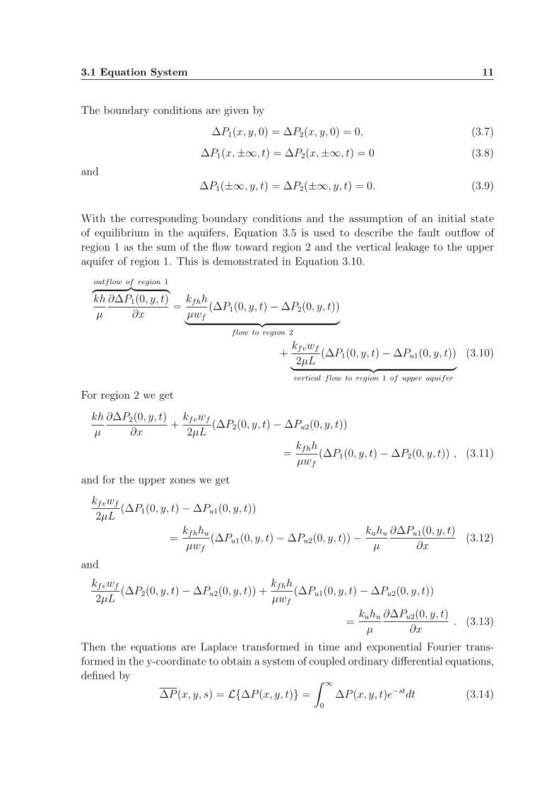
The boundary conditions are given by
∆P1(x, y, 0) = ∆P2(x, y, 0) = 0, (3.7)
∆P1(x,±∞, t) = ∆P2(x,±∞, t) = 0 (3.8)
and
∆P1(±∞, y, t) = ∆P2(±∞, y, t) = 0. (3.9)
With the corresponding boundary conditions and the assumption of an initial state
of equilibrium in the aquifers, Equation 3.5 is used to describe the fault outflow of
region 1 as the sum of the flow toward region 2 and the vertical leakage to the upper
aquifer of region 1. This is demonstrated in Equation 3.10.
outflow of region 1︷ ︸︸ ︷kh
µ
∂∆P1(0, y, t)
∂x=kfhh
µwf
(∆P1(0, y, t)−∆P2(0, y, t))︸ ︷︷ ︸flow to region 2
+kfvwf
2µL(∆P1(0, y, t)−∆Pu1(0, y, t))︸ ︷︷ ︸
vertical flow to region 1 of upper aquifer
(3.10)
For region 2 we get
kh
µ
∂∆P2(0, y, t)
∂x+kfvwf
2µL(∆P2(0, y, t)−∆Pu2(0, y, t))
=kfhh
µwf
(∆P1(0, y, t)−∆P2(0, y, t)) , (3.11)
and for the upper zones we get
kfvwf
2µL(∆P1(0, y, t)−∆Pu1(0, y, t))
=kfhhuµwf
(∆Pu1(0, y, t)−∆Pu2(0, y, t))−kuhuµ
∂∆Pu1(0, y, t)
∂x(3.12)
and
kfvwf
2µL(∆P2(0, y, t)−∆Pu2(0, y, t)) +
kfhh
µwf
(∆Pu1(0, y, t)−∆Pu2(0, y, t))
=kuhuµ
∂∆Pu2(0, y, t)
∂x. (3.13)
Then the equations are Laplace transformed in time and exponential Fourier trans-
formed in the y-coordinate to obtain a system of coupled ordinary differential equations,
defined by
∆P (x, y, s) = L{∆P (x, y, t)} =
∫ ∞0
∆P (x, y, t)e−stdt (3.14)
3.1 Equation System 12
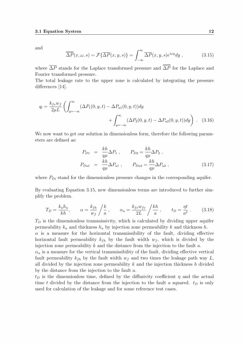
and
∆P (x, ω, s) = F{∆P (x, y, s)} =
∫ ∞−∞
∆P (x, y, s)eiωydy , (3.15)
where ∆P stands for the Laplace transformed pressure and ∆P for the Laplace and
Fourier transformed pressure.
The total leakage rate to the upper zone is calculated by integrating the pressure
differences [14].
ql =kfvwf
2µL
(∫ ∞y=−∞
(∆P1(0, y, t)−∆Pu1(0, y, t))dy
+
∫ ∞y=−∞
(∆P2(0, y, t)−∆Pu2(0, y, t))dy
). (3.16)
We now want to get our solution in dimensionless form, therefore the following param-
eters are defined as:
PD1 =kh
qµ∆P1 , PD2 =
kh
qµ∆P2 ,
PDu1 =kh
qµ∆Pu1 , PDu2 =
kh
qµ∆Pu2 , (3.17)
where PDi stand for the dimensionless pressure changes in the corresponding aquifer.
By evaluating Equation 3.15, new dimensionless terms are introduced to further sim-
plify the problem.
TD =kuhukh
, α =kfhwf
/k
a, αu =
kfvwfv
2L
/kh
a, tD =
ηt
a2. (3.18)
TD is the dimensionless transmissivity, which is calculated by dividing upper aquifer
permeability ku and thickness hu by injection zone permeability k and thickness h.
α is a measure for the horizontal transmissibility of the fault, dividing effective
horizontal fault permeability kfh by the fault width wf , which is divided by the
injection zone permeability k and the distance from the injection to the fault a.
αu is a measure for the vertical transmissibility of the fault, dividing effective vertical
fault permeability kfh by the fault width wf and two times the leakage path way L,
all divided by the injection zone permeability k and the injection thickness h divided
by the distance from the injection to the fault a.
tD is the dimensionless time, defined by the diffusivity coefficient η and the actual
time t divided by the distance from the injection to the fault a squared. tD is only
used for calculation of the leakage and for some reference test cases.
3.2 Fourier and Laplace transform and inversion 13
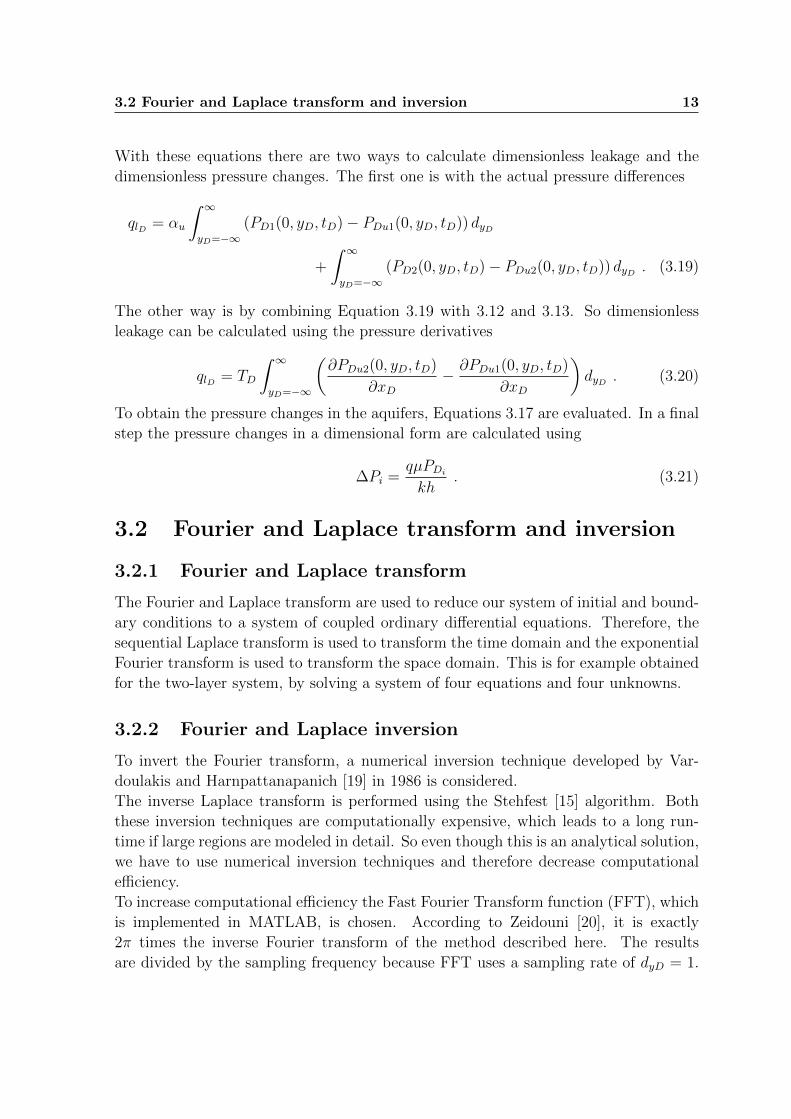
With these equations there are two ways to calculate dimensionless leakage and the
dimensionless pressure changes. The first one is with the actual pressure differences
qlD = αu
∫ ∞yD=−∞
(PD1(0, yD, tD)− PDu1(0, yD, tD)) dyD
+
∫ ∞yD=−∞
(PD2(0, yD, tD)− PDu2(0, yD, tD)) dyD . (3.19)
The other way is by combining Equation 3.19 with 3.12 and 3.13. So dimensionless
leakage can be calculated using the pressure derivatives
qlD = TD
∫ ∞yD=−∞
(∂PDu2(0, yD, tD)
∂xD− ∂PDu1(0, yD, tD)
∂xD
)dyD . (3.20)
To obtain the pressure changes in the aquifers, Equations 3.17 are evaluated. In a final
step the pressure changes in a dimensional form are calculated using
∆Pi =qµPDi
kh. (3.21)
3.2 Fourier and Laplace transform and inversion
3.2.1 Fourier and Laplace transform
The Fourier and Laplace transform are used to reduce our system of initial and bound-
ary conditions to a system of coupled ordinary differential equations. Therefore, the
sequential Laplace transform is used to transform the time domain and the exponential
Fourier transform is used to transform the space domain. This is for example obtained
for the two-layer system, by solving a system of four equations and four unknowns.
3.2.2 Fourier and Laplace inversion
To invert the Fourier transform, a numerical inversion technique developed by Var-
doulakis and Harnpattanapanich [19] in 1986 is considered.
The inverse Laplace transform is performed using the Stehfest [15] algorithm. Both
these inversion techniques are computationally expensive, which leads to a long run-
time if large regions are modeled in detail. So even though this is an analytical solution,
we have to use numerical inversion techniques and therefore decrease computational
efficiency.
To increase computational efficiency the Fast Fourier Transform function (FFT), which
is implemented in MATLAB, is chosen. According to Zeidouni [20], it is exactly
2π times the inverse Fourier transform of the method described here. The results
are divided by the sampling frequency because FFT uses a sampling rate of dyD = 1.
3.2 Fourier and Laplace transform and inversion 14
Finally, our results are shifted using fftshift in MATLAB to ensure that the zero-
frequency component is at the center.
For a more detailed explanation of the inversion techniques, please take a look into
Appendix B of Zeidouni [20].
Chapter 4
Scenarios
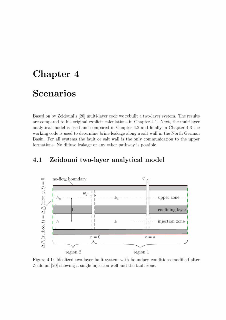
Based on by Zeidouni’s [20] multi-layer code we rebuilt a two-layer system. The results
are compared to his original explicit calculations in Chapter 4.1. Next, the multilayer
analytical model is used and compared in Chapter 4.2 and finally in Chapter 4.3 the
working code is used to determine brine leakage along a salt wall in the North German
Basin. For all systems the fault or salt wall is the only communication to the upper
formations. No diffuse leakage or any other pathway is possible.
4.1 Zeidouni two-layer analytical model
wf
no-flow boundary
∆P2(x,±∞,t
)=
∆P2(±∞,y,t
)=
0 q
x = 0 x = a
region 2 region 1
k
ku
L
upper zone
injection zone
confining layer
h
hu
Figure 4.1: Idealized two-layer fault system with boundary conditions modified after
Zeidouni [20] showing a single injection well and the fault zone.
4.1 Zeidouni two-layer analytical model 16
4.1.1 Boundary conditions
The system has a no-flow boundary condition at the top and the bottom of the system,
as well as insignificant pressure changes towards the infinite lateral boundaries. There
is a single fault splitting the system in regions 1 (with injection) and 2.
Figure 4.1 shows the system and Table 4.1 gives all the input parameters for this test
case. The exact parameters are chosen to match the test cases of Zeidouni [20] and
Shan et al. [14]. The fault width is assumed to be 1.68 meters. This is the value
given by Zeidouni and is supported by Porse [13] who assumes an arbitrary value of
1.68 meters for Hastings field, Texas.
Parameter Value
Injection rate q 0.005 m3
s
Injection well - fault distance a 100 m
Fluid viscosity µ 0.001 kgms
Injection aquifer diffusivity coefficient η 10 m2
s
Injection aquifer permeability k 1 · 10−11 m2
Injection aquifer thickness h 20 m
Upper aquifer diffusivity coefficient ηu 10 m2
s
Upper aquifer permeability ku 1 · 10−11 m2
Upper aquifer thickness hu 20 m
Time (logarithmic & dimensionless) t 10−1 − 106
Table 4.1: Input parameters for the two-layer analytical model.
4.1.2 Leakage rate to the upper aquifer for different values
of αu
We want to compare different values for αu, considering zero pressure change in the
upper aquifer. As previously defined in Equation 3.18, αu is a measure for resistance
that stands for the fault properties divided by the injection zone properties.
In this specific test case, Zeidouni’s code [20] is compared to Shan et al.’s [14] solution.
To get the same results we have to consider a Dirichlet boundary condition of insignif-
icant resistance to flow in the upper aquifer. TD, defined in Equation 3.18, has to be
set to TD → ∞ for the Dirichlet boundary condition. We achieve this by setting the
dimensionless transmissivity TD to a value of 109 in the code.
4.1 Zeidouni two-layer analytical model 17
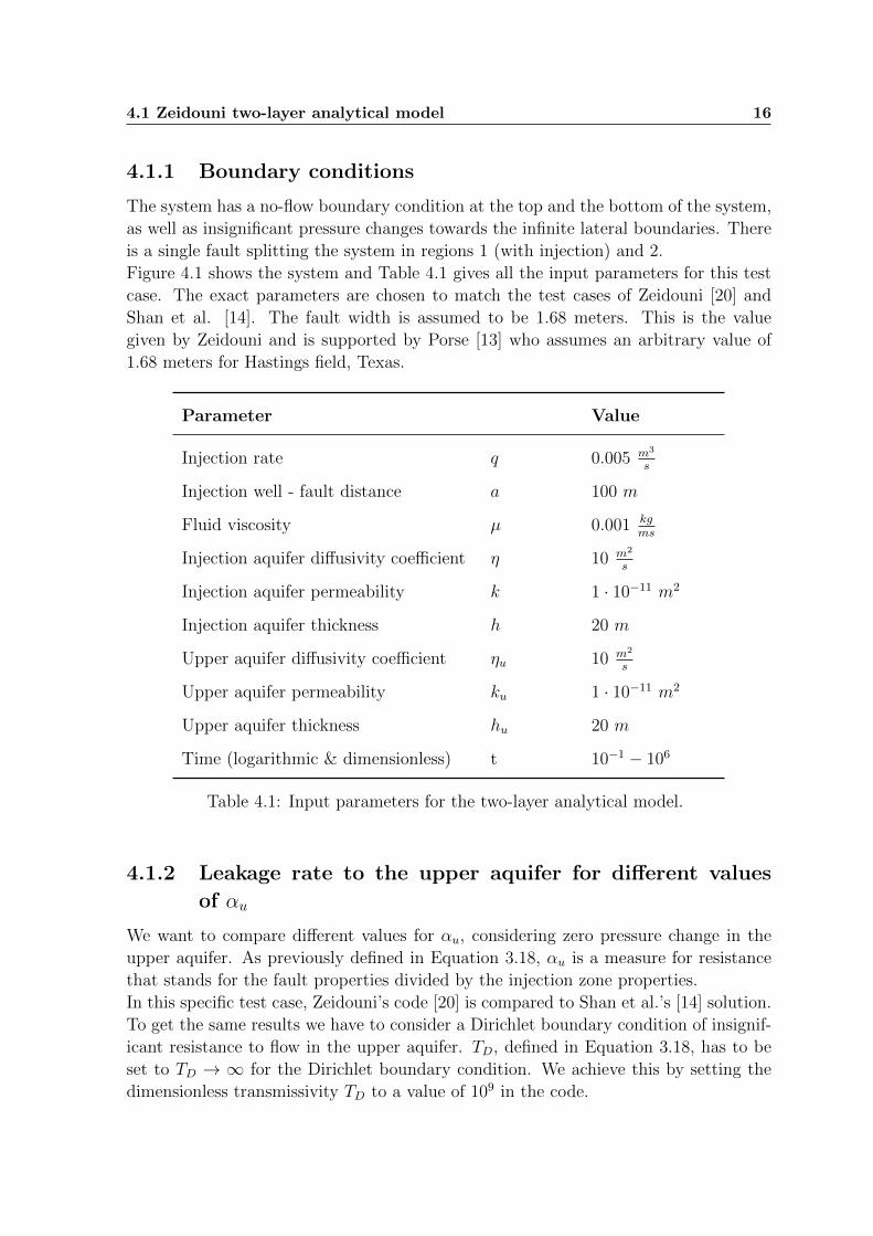
The results of the dimensionless leakage, defined by the leakage to the upper formation
divided by the injection rate, are plotted over dimensionless time tD and compared to
Shan et al.’s [14] solutions in Figure 4.2.
10−1
100
101
102
103
104
105
106
0
0.1
0.2
0.3
0.4
0.5
0.6
0.7
0.8
0.9
1
Time tD [−]
lea
ka
ge
ql /
in
jectio
n r
ate
qIn
j = q
lD [
−]
Dimensionless leakage depending on αu
αu = 0.01
αu = 0.1
αu = 1
αu = 10
Shan reference
Figure 4.2: Dimensionless leakage rate qlD using different values for αu (measure of
fault transmissibility), considering zero pressure change in the upper aquifer.
It is clearly visible, that there is almost perfect agreement to Shan et al.’s [14] solution
for all values of αu. Only for the first couple of time steps a minor difference is visible.
As we can see, increasing αu results in an increased dimensionless leakage rate qlD.
With increased qlD, the steady state of qlD = 1 is reached faster. This implies that, if
we wait long enough, 100 % of the injected fluid flows through the fault. It is obvious
that this does not reflect most real systems. This is why reaching qlD = 1 only makes
sense in this theoretical test case with the dimensionless transmissivity TD set to 109.
The minor differences, especially in the beginning and towards the end of the injection
period can be neglected here. They can probably be traced back to a much higher
resolution used by Shan et al. [14] for his calculations.
4.1 Zeidouni two-layer analytical model 18
4.1.3 Pressure change in the aquifers
In this section, pressure changes ∆P due to injection and leakage in the respective
aquifers are evaluated after 10 hours of injection. Zeidouni [20] once again uses
Shan et al.’s [14] solution to validate his results. Shan et al. calculate the drawdown
of a pumped aquifer and plot the depletion curves for a constant-head fault, a leaky
fault, and no fault at all, which results in a solution developed by Theis [17].
It is interesting to see that the drawdown of the leaky fault scenario is between the
other two curves. The Theis solution is achieved by not allowing vertical flow up
the fault zone, which reduces the system to a simple pumping test. Usually the
Theis solution is used during a aquifer or pumping test with a fully penetrating well.
Therefore, it is reasonable that for a system with no fault, Shan et al. get the Theis
solution. The Theis solution is often used for different type of tests today, namely to
create a Theis type curve. The aquifer properties are evaluated for the unsteady flow
phase of a pumping test to determine the hydraulic properties of a nonleaky aquifer.
The effect of horizontal resistance between the aquifers or regions might be of interest
for the pressure analysis. Zeidouni does account for horizontal resistance in some of his
results at first, but later shows that “for mere calculation of leakage rate, the lateral
resistance of the fault plane can be neglected” [20, Paragraph 23]. Since our focus is
on modeling the pressure changes with the already existing code for modeling leakage,
we do not account for horizontal resistance in our code. Zeidouni does give the explicit
equations for PDiin Paragraph 17 - 20 of his paper [20], which could be used for
future two-layer test cases. Since they are only given for the two-layer system and do
not present any new information, we refrain from using or comparing to them in this
thesis.
Pressure change in the injection aquifer not accounting for horizontal resis-
tance
Not accounting for horizontal resistance leads to a pressure plot with no discontinu-
ities at the fault. The system setup is the same as before, where αu = α = 1 and
the resistance to flow in the upper aquifer is TD = 1. Taking a look at the results in
Figure 4.3, we see that the pressure in the respective aquifer systems matches perfectly
with Zeidouni’s solution [20]. A minimal difference is visible at the fault. This might
be a result of different fault parameters or inaccuracies trying to get the data out of
Zeidouni’s plot with multiple scenarios plotted in just one figure.
The largest pressure change is at the injection site with more than 21 kPa. It decreases
towards the outer boundaries. The left side towards the fault decreases a little faster
due to the leakage through the fault. The faster decrease can also be measured by the
pressure changes in the upper aquifer. The increase in the upper aquifer is proportional
to the faster decrease on the left side of the injection site. The pressure at the right side
drops slower and reaches a steady state for the outer boundaries. There are no disconti-
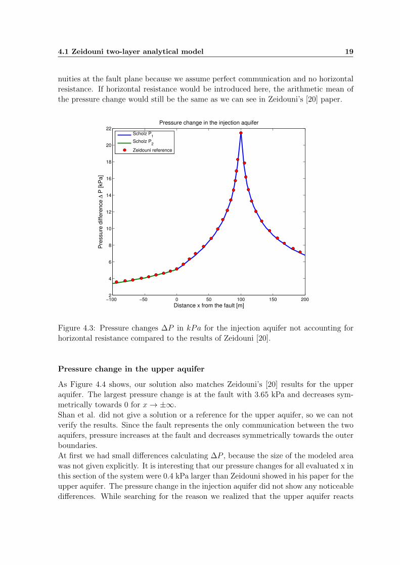
4.1 Zeidouni two-layer analytical model 19
nuities at the fault plane because we assume perfect communication and no horizontal
resistance. If horizontal resistance would be introduced here, the arithmetic mean of
the pressure change would still be the same as we can see in Zeidouni’s [20] paper.
−100 −50 0 50 100 150 2002
4
6
8
10
12
14
16
18
20
22
Distance x from the fault [m]
Pre
ssu
re d
iffe
ren
ce
∆ P
[kP
a]
Pressure change in the injection aquifer
Scholz P
1
Scholz P2
Zeidouni reference
Figure 4.3: Pressure changes ∆P in kPa for the injection aquifer not accounting for
horizontal resistance compared to the results of Zeidouni [20].
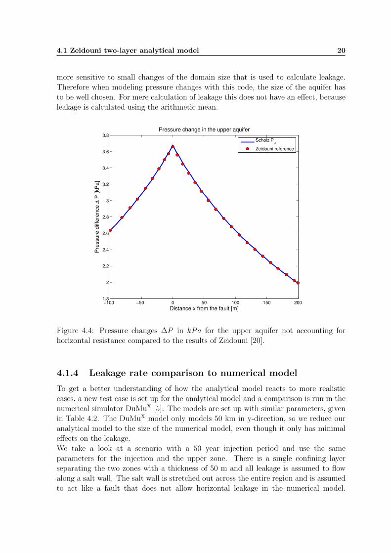
Pressure change in the upper aquifer
As Figure 4.4 shows, our solution also matches Zeidouni’s [20] results for the upper
aquifer. The largest pressure change is at the fault with 3.65 kPa and decreases sym-
metrically towards 0 for x→ ±∞.
Shan et al. did not give a solution or a reference for the upper aquifer, so we can not
verify the results. Since the fault represents the only communication between the two
aquifers, pressure increases at the fault and decreases symmetrically towards the outer
boundaries.
At first we had small differences calculating ∆P , because the size of the modeled area
was not given explicitly. It is interesting that our pressure changes for all evaluated x in
this section of the system were 0.4 kPa larger than Zeidouni showed in his paper for the
upper aquifer. The pressure change in the injection aquifer did not show any noticeable
differences. While searching for the reason we realized that the upper aquifer reacts
4.1 Zeidouni two-layer analytical model 20
more sensitive to small changes of the domain size that is used to calculate leakage.
Therefore when modeling pressure changes with this code, the size of the aquifer has
to be well chosen. For mere calculation of leakage this does not have an effect, because
leakage is calculated using the arithmetic mean.
−100 −50 0 50 100 150 2001.8
2
2.2
2.4
2.6
2.8
3
3.2
3.4
3.6
3.8
Distance x from the fault [m]
Pre
ssu
re d
iffe
ren
ce
∆ P
[kP
a]
Pressure change in the upper aquifer
Scholz P
u
Zeidouni reference
Figure 4.4: Pressure changes ∆P in kPa for the upper aquifer not accounting for
horizontal resistance compared to the results of Zeidouni [20].
4.1.4 Leakage rate comparison to numerical model
To get a better understanding of how the analytical model reacts to more realistic
cases, a new test case is set up for the analytical model and a comparison is run in the
numerical simulator DuMuX [5]. The models are set up with similar parameters, given
in Table 4.2. The DuMuX model only models 50 km in y-direction, so we reduce our
analytical model to the size of the numerical model, even though it only has minimal
effects on the leakage.
We take a look at a scenario with a 50 year injection period and use the same
parameters for the injection and the upper zone. There is a single confining layer
separating the two zones with a thickness of 50 m and all leakage is assumed to flow
along a salt wall. The salt wall is stretched out across the entire region and is assumed
to act like a fault that does not allow horizontal leakage in the numerical model.
4.1 Zeidouni two-layer analytical model 21
Therefore, we double the initial fault width of 50 m and consider only one region in
the analytical model. As previously mentioned in Section 2.1 and 4.1.3, the horizontal
resistance does not have an effect on the leakage.
Parameter Value
Injection rate q 0.02175 m3
s
Injection well - fault distance a 5000 m
Fluid viscosity µ 0.001 kgms
Aquifer diffusivity coefficients η 0.55556 m2
s
Aquifer permeabilities k 1 · 10−13 m2
Aquifer thicknesses h 50 m
Salt Wall / Fault permeability kf 1 · 10−12 m2
Injection period t 50 years
Table 4.2: Input parameters for the two-layer analytical model compared to the nu-
merical model.
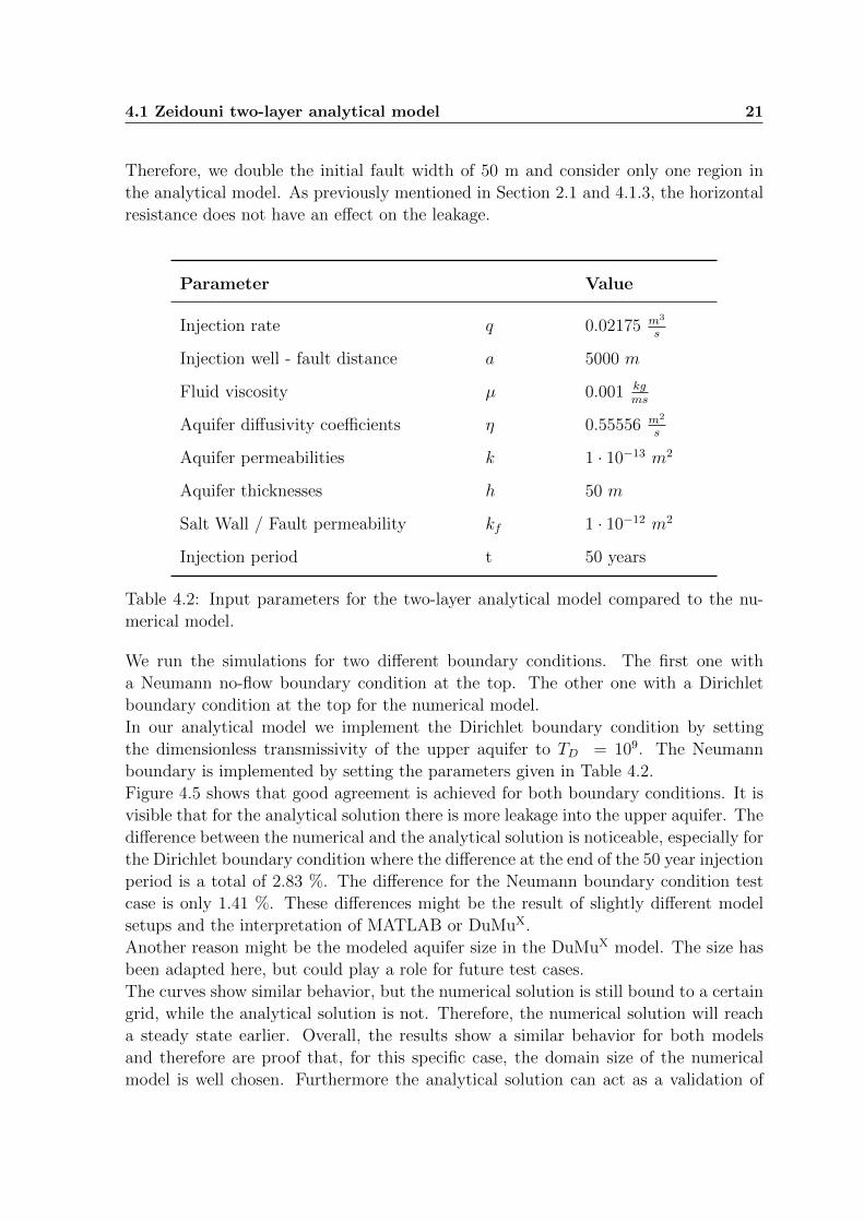
We run the simulations for two different boundary conditions. The first one with
a Neumann no-flow boundary condition at the top. The other one with a Dirichlet
boundary condition at the top for the numerical model.
In our analytical model we implement the Dirichlet boundary condition by setting
the dimensionless transmissivity of the upper aquifer to TD = 109. The Neumann
boundary is implemented by setting the parameters given in Table 4.2.
Figure 4.5 shows that good agreement is achieved for both boundary conditions. It is
visible that for the analytical solution there is more leakage into the upper aquifer. The
difference between the numerical and the analytical solution is noticeable, especially for
the Dirichlet boundary condition where the difference at the end of the 50 year injection
period is a total of 2.83 %. The difference for the Neumann boundary condition test
case is only 1.41 %. These differences might be the result of slightly different model
setups and the interpretation of MATLAB or DuMuX.
Another reason might be the modeled aquifer size in the DuMuX model. The size has
been adapted here, but could play a role for future test cases.
The curves show similar behavior, but the numerical solution is still bound to a certain
grid, while the analytical solution is not. Therefore, the numerical solution will reach
a steady state earlier. Overall, the results show a similar behavior for both models
and therefore are proof that, for this specific case, the domain size of the numerical
model is well chosen. Furthermore the analytical solution can act as a validation of
4.1 Zeidouni two-layer analytical model 22
0 10 20 30 40 50 60 70 80 90 1000
0.1
0.2
0.3
0.4
0.5
0.6
0.7
0.8
0.9
1
Flux into shallow aquifers along salt wall
Ma
ss F
low
Ra
te /
In
jectio
n R
ate
[−
]
Time [years]
DuMuX Neumann
DuMuX Dirichlet
Analytical Neumann
Analytical Dirichlet
Figure 4.5: Dimensionless leakage rate qlD comparison to numerical model for an equiv-
alent two-layer reference system set up in DuMuX.
the numerical solution. Both describe the problem quite well and the small differences
can be subject of future research.
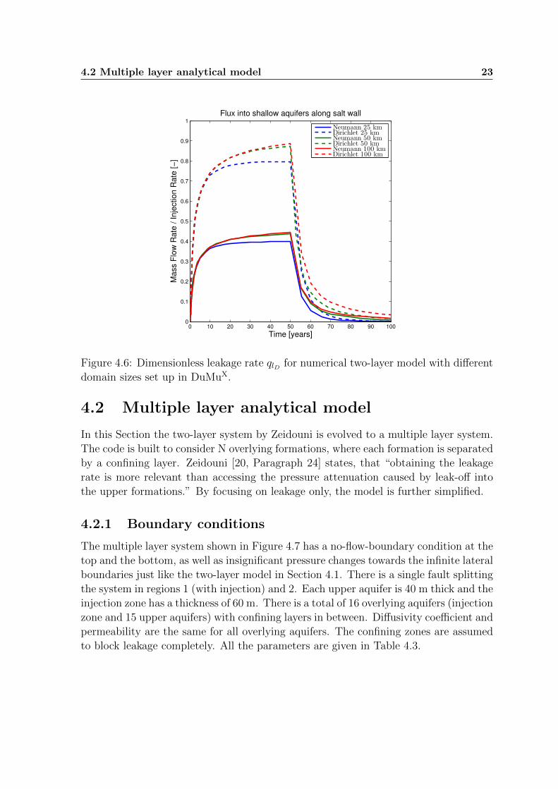
As described earlier, the size of the modeled area does matter. While the analytical
model is only sensitive to the size when it comes to pressure evaluations, the DuMuX
model shows that the size does have an effect on the leakage in Figure 4.6. A steady
state is reached faster for smaller areas due to the domain size and the Dirichlet bound-
ary conditions set there. Consequently, when modeling large systems, numerical models
would be computationally expensive and might still reach a steady state too early.
4.2 Multiple layer analytical model 23
0 10 20 30 40 50 60 70 80 90 1000
0.1
0.2
0.3
0.4
0.5
0.6
0.7
0.8
0.9
1
Flux into shallow aquifers along salt wall
Ma
ss F
low
Ra
te /
In
jectio
n R
ate
[−
]
Time [years]
Neumann 25 kmDirichlet 25 kmNeumann 50 kmDirichlet 50 kmNeumann 100 kmDirichlet 100 km
Figure 4.6: Dimensionless leakage rate qlD for numerical two-layer model with different
domain sizes set up in DuMuX.
4.2 Multiple layer analytical model
In this Section the two-layer system by Zeidouni is evolved to a multiple layer system.
The code is built to consider N overlying formations, where each formation is separated
by a confining layer. Zeidouni [20, Paragraph 24] states, that “obtaining the leakage
rate is more relevant than accessing the pressure attenuation caused by leak-off into
the upper formations.” By focusing on leakage only, the model is further simplified.
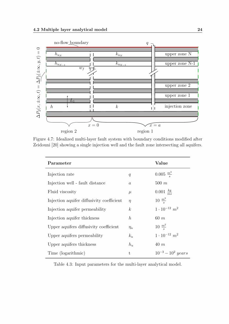
4.2.1 Boundary conditions
The multiple layer system shown in Figure 4.7 has a no-flow-boundary condition at the
top and the bottom, as well as insignificant pressure changes towards the infinite lateral
boundaries just like the two-layer model in Section 4.1. There is a single fault splitting
the system in regions 1 (with injection) and 2. Each upper aquifer is 40 m thick and the
injection zone has a thickness of 60 m. There is a total of 16 overlying aquifers (injection
zone and 15 upper aquifers) with confining layers in between. Diffusivity coefficient and
permeability are the same for all overlying aquifers. The confining zones are assumed
to block leakage completely. All the parameters are given in Table 4.3.
4.2 Multiple layer analytical model 24
wf
no-flow boundary∆P2(x,±∞,t
)=
∆P2(±∞,y,t
)=
0
upper zone 2
L1
q
x = 0 x = a
region 2 region 1
k
kuN
upper zone 1
injection zoneh
huN upper zone N
upper zone N-1huN−1kuN−1
Figure 4.7: Idealized multi-layer fault system with boundary conditions modified after
Zeidouni [20] showing a single injection well and the fault zone intersecting all aquifers.
Parameter Value
Injection rate q 0.005 m3
s
Injection well - fault distance a 500 m
Fluid viscosity µ 0.001 kgms
Injection aquifer diffusivity coefficient η 10 m2
s
Injection aquifer permeability k 1 · 10−12 m2
Injection aquifer thickness h 60 m
Upper aquifers diffusivity coefficient ηu 10 m2
s
Upper aquifers permeability ku 1 · 10−12 m2
Upper aquifers thickness hu 40 m
Time (logarithmic) t 10−3− 102 years
Table 4.3: Input parameters for the multi-layer analytical model.
4.2 Multiple layer analytical model 25
4.2.2 Leakage rate comparison for multi-layer or two-layer
systems
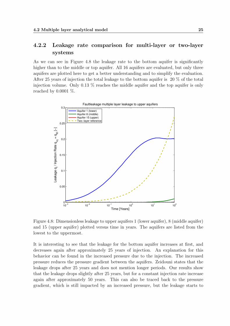
As we can see in Figure 4.8 the leakage rate to the bottom aquifer is significantly
higher than to the middle or top aquifer. All 16 aquifers are evaluated, but only three
aquifers are plotted here to get a better understanding and to simplify the evaluation.
After 25 years of injection the total leakage to the bottom aquifer is 20 % of the total
injection volume. Only 0.13 % reaches the middle aquifer and the top aquifer is only
reached by 0.0001 %.
10−3
10−2
10−1
100
101
102
0
0.05
0.1
0.15
0.2
0.25
0.3
Time [Years]
Le
aka
ge
ql /
In
jectio
n R
ate
qin
j = q
lD [
−]
Faultleakage multiple layer leakage to upper aquifers
Aquifer 1 (lower)
Aquifer 8 (middle)
Aquifer 15 (upper)
Two−layer reference
Figure 4.8: Dimensionless leakage to upper aquifers 1 (lower aquifer), 8 (middle aquifer)
and 15 (upper aquifer) plotted versus time in years. The aquifers are listed from the
lowest to the uppermost.
It is interesting to see that the leakage for the bottom aquifer increases at first, and
decreases again after approximately 25 years of injection. An explanation for this
behavior can be found in the increased pressure due to the injection. The increased
pressure reduces the pressure gradient between the aquifers. Zeidouni states that the
leakage drops after 25 years and does not mention longer periods. Our results show
that the leakage drops slightly after 25 years, but for a constant injection rate increase
again after approximately 50 years. This can also be traced back to the pressure
gradient, which is still impacted by an increased pressure, but the leakage starts to
4.3 North German Basin multiple layer analytical model 26
reach all aquifers by then and is therefore causing changes in the entire model again.
Given these small increases after the initial decrease, the leakage rate is going to reach
a steady state in all aquifers at some point.
The leakage to the middle or uppermost aquifer is relatively small compared to the
leakage into the lowest aquifer. This shows that multiple layers with confining layers
should always be considered. The approach is supported when the equivalent two-layer
system is compared to the multi-layer solution in Figure 4.8.
For the two-layer system the thickness of the upper aquifer is assumed to be 600 m (sum
of all overlying aquifers in the multi-layer system) and the confining layer is assumed
to be 450 m (sum of all confining layers in the multi-layer system). By the end of a
25 year injection period the bottom layer alone has more leakage than the equivalent
two-layer system. This demonstrates how important multiple layers are in hindering
up-fault leakage. Other test scenarios with leakage through abandoned wells e.g. run
by Nordbotten et. al [10] show similar results when it comes to multiple layer systems
with confining layers.
4.3 North German Basin multiple layer analytical
model
In this Section, leakage along a salt wall for a real case scenario is modeled. Several
simplifications and assumptions are made to adapt the real case parameters to our
analytical solution.
All layers are assumed to be homogenous and of constant thickness. The leakage occurs
only through the fault zone, i.e. along the salt wall, which does not reflect the real
scenario, where diffuse leakage through the confining layers takes place.
The results of the analytical solution are compared to a numerical simulation with a
similar setting.
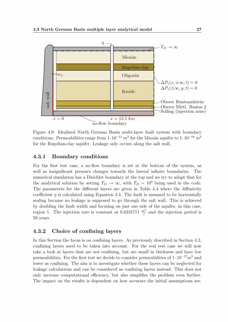
Figure 4.9 shows the idealized system. It illustrates how the boundary conditions are
interpreted. Since the code of the analytical solution does not consider a horizontally
sealing fault and Zeidouni [20] shows in his paper that a horizontally sealing fault does
not have an impact on the system, we still model flow through the fault to both re-
gions but are only interested in leakage to region 1. To achieve a similar setting to the
numerical model, the fault width is doubled and we focus on just one region when it
comes to the evaluation. By doubling the fault width, our leakage along the salt wall
should be the same as in the numerical model.
The real system also has another aquifer on top of the Miozan aquifer, called Quar-
ternary which is considered by the numerical model. For the analytical solution this
is not possible. That is why the two aquifers are summed together, which could be
performed due to their similar properties. However, this would also result in a much
longer fault. Another solution is to only consider the Miozan aquifer and neglect the
Quarternary aquifer.
4.3 North German Basin multiple layer analytical model 27
no-flow boundary
∆P1(x,±∞, t) = 0∆P1(±∞, y, t) = 0
q
x = 0 x = 13.5 km
Solling (injection zone)
Rupelian-clay
Miozan
Oligozan
Kreide
Oberer BuntsandsteinOberer Mittl. Buntss 2
wf
salt
wal
lTD →∞
Figure 4.9: Idealized North German Basin multi-layer fault system with boundary
conditions. Permeabilities range from 1 ·10−13 m2 for the Miozan aquifer to 1 ·10−18 m2
for the Rupelian-clay aquifer. Leakage only occurs along the salt wall.
4.3.1 Boundary conditions
For the first test case, a no-flow boundary is set at the bottom of the system, as
well as insignificant pressure changes towards the lateral infinite boundaries. The
numerical simulation has a Dirichlet boundary at the top and we try to adapt that for
the analytical solution by setting TD → ∞, with TD = 109 being used in the code.
The parameters for the different layers are given in Table 4.4 where the diffusivity
coefficient η is calculated using Equation 3.4. The fault is assumed to be horizontally
sealing because no leakage is supposed to go through the salt wall. This is achieved
by doubling the fault width and focusing on just one side of the aquifer, in this case,
region 1. The injection rate is constant at 0.0235711 m3
sand the injection period is
50 years.
4.3.2 Choice of confining layers
In this Section the focus is on confining layers. As previously described in Section 4.2,
confining layers need to be taken into account. For the real test case we will now
take a look at layers that are not confining, but are small in thickness and have low
permeabilities. For the first test we decide to consider permeabilities of 1 ·10−17m2 and
lower as confining. The aim is to investigate whether these layers can be neglected for
leakage calculations and can be considered as confining layers instead. This does not
only increase computational efficiency, but also simplifies the problem even further.
The impact on the results is dependent on how accurate the initial assumptions are.
4.3 North German Basin multiple layer analytical model 28
Layer Thickness h Diffusivity
coefficient η
Permeability k
Tertiary Post-Rupelian
(Miozan)
400 m 1.481 m2
s1 · 10−13 m2
Rupelian-clay 80 m 2.222 · 10−5 m2
s1 · 10−18 m2
Oligozan, Eozan, Palaozan 350 m 2.222 m2
s1 · 10−13 m2
Kreide 900 m 0.317 m2
s1 · 10−14 m2
Oberer Buntsandstein 50 m 5.556 · 10−4 m2
s1 · 10−17 m2
Oberer Mittl. Buntss 2 20 m 5.556 · 10−3 m2
s1 · 10−16 m2
Solling (injection zone) 20 m 1.222 m2
s1.1 · 10−13 m2
Table 4.4: Layer properties for the North German Basin multiple layer analytical
model.
Therefore these further assumptions should be handled with care and should only
have a minimal impact on the results.
0 5 10 15 20 25 30 35 40 45 500
0.05
0.1
0.15
0.2
0.25
0.3
0.35
0.4
North German Basin without confining layers
Time [years]
Mass F
low
R
ate
ql /
Inje
ction R
ate
qin
j = q
lD [−
]
Oberer Mittl Buntss 2
Oberer Buntsandstein
Kreide
Oligozän
Rupelian−clay
Miozän
(a) North German Basin multi-layer all layers
with real parameters.
0 5 10 15 20 25 30 35 40 45 500
0.05
0.1
0.15
0.2
0.25
0.3
0.35
0.4
North German Basin with confining layers
Time [years]
Mass F
low
R
ate
ql /
Inje
ction R
ate
qin
j = q
lD [−
]
Oberer Mittl Buntss 2
Kreide
Oligozän
Miozän
(b) North German Basin multi-layer with some
layers defined as confining.
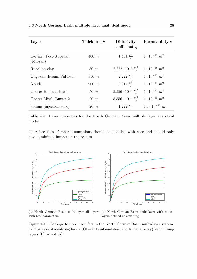
Figure 4.10: Leakage to upper aquifers in the North German Basin multi-layer system.
Comparison of idealizing layers (Oberer Buntsandstein and Rupelian-clay) as confining
layers (b) or not (a).
4.3 North German Basin multiple layer analytical model 29
Figure 4.10 a) and b) show that the leakage to the relatively thick aquifers is almost the
same for calculations which take the aquifers into account and for calculations which
consider them as confining layers. For both test cases 36 % of the total leakage are in
the top aquifer “Miozan” by the end of the 50 year injection period. The “Kreide” and
“Oligozan” aquifer also match perfectly. Only 0.019 % of the leakage migrates into the
“Rupelian-clay” aquifer by the end of the 50 year injection period. The assumption
of considering the above mentioned aquifers as confining in this scenario seems to be
valid.
The bottom aquifer “Oberer Mittl. Buntss 2” could probably be considered as confining
as well for future scenarios. In this study, we decided on keeping the properties, because
it is the first aquifer above the injection zone, and for small and short injections the
aquifer might become more important.
4.3.3 Leakage rate comparison
The analytical solution is plotted and compared to a numerical simulation run in
DuMuX [5]. We now use the results of the confining layers from Section 4.3.2 to
simplify the calculations. A new compressibility ct = 9 · 10−10 1Pa
is introduced for the
comparison to the numerical model. Therefore, the diffusivity coefficients in Table 4.4
need to be recalculated for this case with Equation 3.4. Since the initial compressibility
was set to ct = 4.5 · 10−10 1Pa
, the diffusivity coefficients need to be divided by 2. For
this case only the leakage to the uppermost aquifer is plotted.
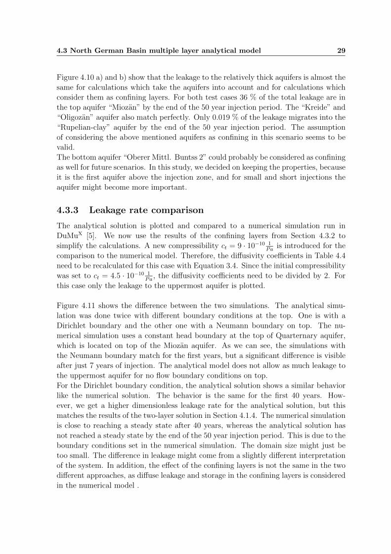
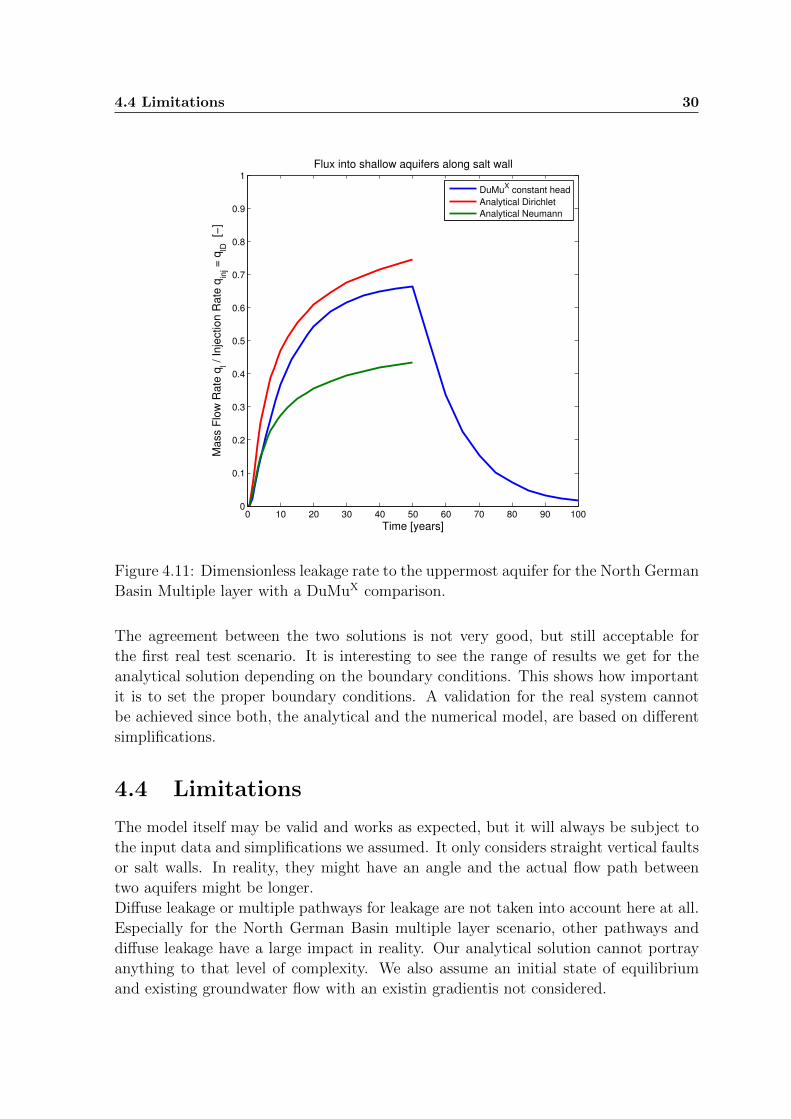
Figure 4.11 shows the difference between the two simulations. The analytical simu-
lation was done twice with different boundary conditions at the top. One is with a
Dirichlet boundary and the other one with a Neumann boundary on top. The nu-
merical simulation uses a constant head boundary at the top of Quarternary aquifer,
which is located on top of the Miozan aquifer. As we can see, the simulations with
the Neumann boundary match for the first years, but a significant difference is visible
after just 7 years of injection. The analytical model does not allow as much leakage to
the uppermost aquifer for no flow boundary conditions on top.
For the Dirichlet boundary condition, the analytical solution shows a similar behavior
like the numerical solution. The behavior is the same for the first 40 years. How-
ever, we get a higher dimensionless leakage rate for the analytical solution, but this
matches the results of the two-layer solution in Section 4.1.4. The numerical simulation
is close to reaching a steady state after 40 years, whereas the analytical solution has
not reached a steady state by the end of the 50 year injection period. This is due to the
boundary conditions set in the numerical simulation. The domain size might just be
too small. The difference in leakage might come from a slightly different interpretation
of the system. In addition, the effect of the confining layers is not the same in the two
different approaches, as diffuse leakage and storage in the confining layers is considered
in the numerical model .
4.4 Limitations 30
0 10 20 30 40 50 60 70 80 90 1000
0.1
0.2
0.3
0.4
0.5
0.6
0.7
0.8
0.9
1
Flux into shallow aquifers along salt wall
Ma
ss F
low
Ra
te q
l / I
nje
ctio
n R
ate
qin
j = q
lD
[−]
Time [years]
DuMuX constant head
Analytical Dirichlet
Analytical Neumann
Figure 4.11: Dimensionless leakage rate to the uppermost aquifer for the North German
Basin Multiple layer with a DuMuX comparison.
The agreement between the two solutions is not very good, but still acceptable for
the first real test scenario. It is interesting to see the range of results we get for the
analytical solution depending on the boundary conditions. This shows how important
it is to set the proper boundary conditions. A validation for the real system cannot
be achieved since both, the analytical and the numerical model, are based on different
simplifications.
4.4 Limitations
The model itself may be valid and works as expected, but it will always be subject to
the input data and simplifications we assumed. It only considers straight vertical faults
or salt walls. In reality, they might have an angle and the actual flow path between
two aquifers might be longer.
Diffuse leakage or multiple pathways for leakage are not taken into account here at all.
Especially for the North German Basin multiple layer scenario, other pathways and
diffuse leakage have a large impact in reality. Our analytical solution cannot portray
anything to that level of complexity. We also assume an initial state of equilibrium
and existing groundwater flow with an existin gradientis not considered.
Chapter 5
Summary
Over the last 10 to 20 years, there has been rising interest in ways to use the subsurface.
Most of these projects are motivated by the changing atmospheric composition and
the demand to use or store energy. Multiple possible scenarios of injection into the
subsurface are subject of current research in Germany. Especially the North German
Basin, which consists of special rock formations like salt diapirs and salt walls, is
of interest. These salt walls could act like a fault and be a possible pathway for
migration of injection induced leakage to shallow aquifers. If a fluid is injected into
a deep aquifer, brine or other fluids could migrate to shallow aquifers and possibly
contaminate ground water resources. The aim of this thesis is to model the leakage
along a salt wall to upper formations analytically to compare and validate existing
numerical models.
Since there is no explicit analytical model for leakage along a salt wall, a model for
leakage through a fault, developed by Zeidouni [20], is used. This basic model is
checked and compared to other simple two-layer reference cases and numerical models.
Then multiple layers are introduced and finally, a more realistic multiple layer system
of the North German Basin is modeled and compared to the numerical simulations
run with DuMuX [5].
For the first step, the aim was to validate a simple two-layer solution. This was done by
using Zeidouni’s approach and Shan et al.’s solution as well as a numerical solution. The
different models were set up similarly and all started with an initial state of equilibrium.
The analytical solution by Zeidouni shows good agreement to all the reference models.
The effect of different parameters was investigated and the simplifications introduced
by Zeidouni were found to be accurate for this specific test case. It is interesting to
see that the leakage to upper aquifers is independent of the horizontal fault properties.
We use this solution to model leakage along a salt wall, which is described as a fault
that only allows leakage to one side of the fault in our context. Pressure evaluation of
the the injection zone and the upper aquifer for the two-layer model showed that the
pressure changes in the aquifers are extremely sensitive to the domain size.
32
The next step was done by introducing multiple layers with multiple confining zones
that do not allow any leakage. The results were compared to an equivalent two-layer
system. Like Zeidouni, we found the difference between single and multiple layer
models were significant. After a short injection period of 20 years, the model already
shows that the confining layers hinder upfault leakage extremely. When modeling real
systems with confining layers or strongly varying parameters, multiple layers need to
be considered for future simulations.
Finally, the real parameters of the North German Basin were used with the analytical
model for multiple layers. Many simplifications and assumptions of the physics were
needed to describe the real system. The analytical model showed quite close agreement
to the numerical simulation, but differences, depending on the top boundary condition,
were identified. The boundary conditions for the analytical and the numerical model
cannot be set exactly the same due to the different approaches. The numerical model
also considers diffuse leakage and storage in the confining layers and the analytical
model does not. The results are good enough to show that there is some agreement, but
the models need further investigation, especially concerning the boundary conditions.
A big advantage of the analytical model can be seen when modeling large areas. The
numerical model is always bound to a certain domain size, whereas the analytical model
theoretically stretches out towards infinity. This can be seen for the last years of the
injection period when the numerical model is about to reach a steady state, because
the model boundaries set by the domain size are reached faster.
All in all, the analytical model developed by Zeidouni, which is presented in this thesis,
validates the results of numerical models developed in DuMuX, but the results do not
match perfectly yet, which needs to be further investigated. The effect of the confining
layers for multiple layer system or real scenarios is found to be important and the
boundary conditions need to be well chosen.
Chapter 6
Outlook
This thesis showed how powerful analytical solutions can be for modeling leakage. Some
of the disadvantages concerning the analytical model where also shown, but since com-
putational efficiency is very important, analytical models should be subject of further
research. This is especially true for regions with leaky faults or needing a risk analysis.
Analytical models have a lot of advantages considering efficiency, but they are based
on various assumptions and simplifications.
Analytical solution for fault leakage should be further investigated. Based on the lim-
itations of analytical solutions presented here, a new approach with multiple faults or
old wells is of interest. Real systems often show multiple possible pathways for leakage
to upper formations. Therefore, when modeling real scenarios, these pathways should
be portrayed in the analytical solution. Inhomogeneous fault zones and a more detailed
fault structure, as well as fault zones with an angle, are of interest too. The fault zones
are assumed to be homogenous and vertical. For the real system, they are everything
but homogenous and most of the time they do have an angle. Therefore, separating
the fault zone into different sections could help improve the results.
As one of the most important subjects of future research, diffuse leakage needs to be
investigated. The effect of the confining layers was shown in this thesis, but we know
that for the real system diffuse leakage can be important. Where numerical models can
easily take diffuse leakage into account, the analytical model needs a new approach.
Cihan et al. [4] developed an analytical solution that takes diffuse leakage into account.
Due to the fact that some layers are not separated perfectly by a confining layer, diffuse
leakage, especially for large scenarios, is extremely important.
Finally, the analytical solution can not only validate existing numerical models, but
could also be coupled with an existing model. For large scale calculations, the advan-
tages of the analytical solution are obvious. But a complex fault structure or inhomo-
geneous sediments surrounding the salt wall are best portrayed by a detailed numerical
solution. Taking the advantages of both could result in a coupled model which uses
the analytical solution for the regions far from the salt wall and the numerical model
for the complex structures around the salt wall.
Bibliography
[1] Birkholzer, J. T. and Zhou, Q. Basin-scale hydrogeologic impacts of CO2 storage:
Capacity and regulatory implications. International Journal of Greenhouse Gas
Control, 3(6):745–756, Dec 2009.
[2] Caine, J., Evans, J., and Forster, C. Fault zone architecture and permeability
structure. Geology, 24(11):1025–1028, Nov 1996.
[3] Cihan, A., Birkholzer, J. T., and Zhou, Q. Pressure buildup and brine migration
during CO2 storage in multilayered aquifers. Groundwater, 51(2):252–267, 2013.
[4] Cihan, A., Zhou, Q., and Birkholzer, J. T. Analytical solutions for pressure
perturbation and fluid leakage through aquitards and wells in multilayered-aquifer
systems. Water Resources Research, 47(10), 2011.
[5] Flemisch, B., Darcis, M., Erbertseder, K., Faigle, B., Lauser, A., Mosthaf, K.,
Muething, S., Nuske, P., Tatomir, A., Wolff, M., and Helmig, R. DuMu(x):
DUNE for multi-{phase, component, scale, physics, ...} flow and transport in
porous media. Advances in Water Resources, 34(9, SI):1102–1112, Sep 2011.
[6] Houghton, J., Ding, Y., Griggs, D., Noguer, M., van der Linden, P., Dai, X.,
Maskell, K., and Johnson, C. Climate Change 2001: The Scientific Basis. Con-
tribution of Working Group I to the Third Assessment Report of the Intergov-
ernmental Panel on Climate Change. Cambridge University Press, Cambridge,
United Kingdom and New York, NY, USA, 2001.
[7] Kang, M., Nordbotten, J. M., Doster, F., and Celia, M. A. Analytical solutions
for two- phase subsurface flow to a leaky fault considering vertical flow effects and
fault properties. Water Resources Research, 50(4):3536–3552, Apr 2014.
[8] Metz, B. and on Climate Change. Working Group III., I. P. Carbon Dioxide
Capture and Storage: Special Report of the Intergovernmental Panel on Climate
Change. Cambridge University Press, 2005.
[9] Nicot, J.-P. Evaluation of large-scale CO2 storage on fresh-water sections of
aquifers: An example from the Texas Gulf Coast Basin. International Journal
34
BIBLIOGRAPHY 35
of Greenhouse Gas Control, 2(4, SI):582–593, Oct 2008. 4th Trondheim Confer-
ence on CO2 Capture, Transport and Storage, Trondheim, Norway, Oct 16-17,
2007.
[10] Nordbotten, J., Celia, M., and Bachu, S. Analytical solutions for leakage rates
through abandoned wells. Water Resources Research, 40(4), Apr 6 2004.
[11] Oldenburg, C. M., Bryant, S. L., and Nicot, J.-P. Certification framework based
on effective trapping for geologic carbon sequestration. International Journal of
Greenhouse Gas Control, 3(4):444–457, Jul 2009.
[12] Peter, W. B. and Larson, E. E. Putnam’s geology, 1978.
[13] Porse, S. L. Using analytical and numerical modeling to assess deep groundwater
monitoring parameters at carbon capture, utilization, and storage sites. Diplo-
marbeit, The University of Texas at Austin, Dec 2013.
[14] Shan, C., Javandel, I., and Witherspoon, P. A. Characterization of leaky faults:
Study of water flow in aquifer-fault-aquifer systems. Water Resources Research,
31(12):2897–2904, 1995.
[15] Stehfest, H. Algorithm 368: Numerical inversion of laplace transforms [d5]. Com-
mun. ACM, 13(1):47–49, Jan 1970.
[16] Sun, A. Y. and Nicot, J.-P. Inversion of pressure anomaly data for detecting leak-
age at geologic carbon sequestration sites. Advances in Water Resources, 44:20–29,
Aug 2012.
[17] Theis, C. The relation between the lowering of the piezometric surface and the
rate and duration of discharge of a well using ground water storage. Transactions-
American Geophysical Union, 16(2):519–524, Aug 1935.
[18] U.S. Geological Survey. Geophysics of rio grande basins, Aug 2014.
[19] Vardoulakis, I. and Harnpattanapanich, T. Numerical Laplace Fourier-Transform
Inversion Technique for Layered-Soil Consolidation Problems .1. Fundamental-
Solutions and Validation. International Journal for Numerical and Analytical
Methods in Geomechanics, 10(4):347–365, Jul-Aug 1986.
[20] Zeidouni, M. Analytical model of leakage through fault to overlying formations.
Water Resources Research, 48(12), 2012.