Analytical Modeling of Fire Smoke Spread in High-rise Buildings

Dahai Qi

A Thesis Proposal

In the Department

of

Building, Civil and Environmental Engineering

Presented in Partial Fulfillment of the Requirements

for the Degree of Doctor of Philosophy at

Concordia University

Montreal, Quebec, Canada

September 2016

© Dahai Qi, 2016

CONCORDIA UNIVERSITY

School of Graduate Studies

This is to certify that the thesis prepared

By: Dahai Qi

Entitled: Analytical Modeling of Fire Smoke Spread in High-rise Buildings

and submitted in partial fulfillment of the requirements for the degree of

Doctor of Philosophy (Building Engineering)

complies with the regulations of the University and meets the accepted standards with respect to

originality and quality.

Signed by the final Examining Committee:

Chair

Dr. Nematollaah Shiri

External Examiner

Dr. Jie Ji

External to Program

Dr. Marius Paraschivoiu

Examiner

Dr. Samuel Li

Examiner

Dr. Hua Ge

Thesis Supervisor

Dr. Liangzhu (Leon) Wang & Dr. Radu Zmeureanu

Approved by

_________________________________________

Chair of Department or Graduate Program Director

__________________________

Dean of Faculty

iii

Abstract

Analytical Modeling of Fire Smoke Spread in High-rise Buildings

Dahai Qi, Ph.D.

Concordia University, 2016

Canada has a large number of high-rise buildings; according to the National Fire Protection

Association (NFPA) 101 Life Safety Code, a high-rise building is defined as a building with the

height of more than 23 meters or that is roughly 7 stories tall. Fires in high-rise buildings are often

disastrous and cause huge losses if the buildings are not well protected against fires. Historically,

a high-rise fire is more likely to happen in the lower floors according to the statistics. Driven by

stack effect, the resulting smoke from fires may spread to the higher levels more easily via the

vertical shafts, e.g. stairs, elevators, light wells, ventilation ducts, than through leakage openings

in the building structure. It was reported that smoke spread through shafts counts for about 95%

or more of the upward movement of smoke in typical high-rise buildings. Therefore, much

attention has been paid to the study of the smoke movement in vertical shafts.

Analytical models, numerical simulations and experimental studies are the commonly used

methods to study the smoke movement through building shafts. For simplification, most of the

previous studies on the analytical models and numerical simulations assumed adiabatic shaft walls

and did not take heat transfer between smoke and shaft boundaries into consideration. In fact, the

smoke temperature strongly depends on the heat exchange with the shaft walls and may vary

significantly depending on the height. An accurate estimation of the temperature profile in a shaft

iv

is crucial for the prediction of smoke movement during a fire, because the amount of smoke

spreading through a shaft is closely coupled with the heat transfer during a fire. Numerical

approaches normally include CFD model, zone model and mutizone network model, in which the

mutizone network model is often used to study smoke movement during fires in high-rise buildings

but temperature in each zone has to be specified by users due to the lack of energy model, which

may results in errors in stimulation. In addition, full size experiments are often costly and

unpractical to conduct, especially for high-rise buildings. Sub-scale experiment is the often used

one but it lacks sound scaling law to maintain the similarity of scaled and full-size high-rise models.

The main objective of this research is to develop an analytical model and a numerical modeling

approach of coupled heat and mass transfer of fire smoke movement through vertical shafts of

high-rise buildings. Based on the analytical model, simple calculation method and empirical

equation of neutral plane level were developed and validated by experimental data from the

literature. It was found that the empirical equation is more accurate than the existing equation of

neutral plane level. Studies on the dimensionless analytical solutions and similarity study were

also conducted using the analytical model, which provide a new scaling method to sub-scale smoke

spreads in high-rise shafts. The new scaling method was verified by experiments on different size

and material shafts. The results indicated that compared to the common used scaling method,

Froude modeling method, the new scaling method could achieve closer results between sub-scaled

models and the full-size model. The numerical approach is based on a multizone program with an

added energy equation, CONTAM97R, which can calculate the coupled heat and mass transfer

inside the high-rise shafts. Different from floor zoning strategy (FZS) that is frequently used, a

new zoning strategy called adaptive zoning strategy (AZS) was suggested by adapting the

temperature gradient inside the shaft. Using this zoning strategy, a modeling method of smoke

v

movement in shafts during high-rise fires by the mutilizone and energy network program was

proposed. It was concluded that AZS could achieve similar accuracy results as FZS but with fewer

zones.

vi

Acknowledgements

I would like to express my special acknowledgements to my co-supervisor, Dr. Liangzhu (Leon)

Wang, for offering his encouragement and profound knowledge on heat and mass transfer in

buildings. The same acknowledgements to my co-supervisor, Dr. Radu Zmeureanu, whose support

and inspiring suggestions have been precious for the PhD study. Without their guidance and

persistent assistance, this thesis would not have been possible.

I would like to thank the members of examining committee, Dr. Jie Ji, Dr. Marius Paraschivoiu,

Dr. Samuel Li and Dr. Hua Ge, for their precious comments on my thesis work, especially Dr. Jie

Ji for the experimental data from his papers. Without the data, I could not complete the thesis.

Besides, I would also thank my friend and colleague, Guanchao Zhao, who dedicated a lot to the

experiments. He helped me to design, set up and conduct the whole experiments. In addition, I

would like to extend my regards to the rest of my friends and colleagues, Dr. Cheng-Chun Lin,

Weigang Li, Sui Jiang Si Tu, Jun Cheng, Sherif Goubran and Jiaqing He, for their friendship and

knowledge.

Finally, my deepest gratitude goes to my mother, Wenqin Fang, my father, Guangqi Qi, for their

unconditional love and respect for my choices; to my wife, Hui Chen, for her support in realizing

my dreams and our child, Jason, who brings much happiness into my life.

vii

Table of Contents

List of Figures ................................................................................................................................ x

List of Tables .............................................................................................................................. xiv

Nomenclature ............................................................................................................................. xvi

Preface ......................................................................................................................................... xxi

Chapter 1 Introduction ........................................................................................................... 1

1.1. Statement of the problem .............................................................................................................. 3

1.2. Objectives of this thesis ................................................................................................................ 6

1.3. Summary and thesis work introduction ........................................................................................ 7

Chapter 2 Literature Review ............................................................................................... 10

2.1. Introduction ................................................................................................................................. 10

2.2. Analytical models ....................................................................................................................... 12

2.2.1. Analytical model without considering heat transfer ........................................................... 13

2.2.2. Analytical model considering heat transfer ......................................................................... 14

2.3. Scale modeling ............................................................................................................................ 18

2.4. Numerical modeling .................................................................................................................... 21

Chapter 3 Analytical Model of Heat and Mass Transfer through Non-adiabatic High-

rise Shafts during fires ............................................................................................................... 24

3.1. Introduction ................................................................................................................................. 25

3.2. Building shaft with given smoke mass flow rate ........................................................................ 29

3.3. Building shaft with smoke driven by stack effect only ............................................................... 37

3.4. Discussion ................................................................................................................................... 49

3.5. Conclusion .................................................................................................................................. 53

Chapter 4 Dimensionless Analytical Solutions for Steady-state Heat and Mass Transfer

through High-rise Shafts ............................................................................................................ 56

viii

4.1. Introduction ................................................................................................................................. 56

4.2. Theory ......................................................................................................................................... 60

4.2.1. Mechanical smoke venting .................................................................................................. 61

4.2.2. Natural smoke venting ........................................................................................................ 64

4.3. Experiments ................................................................................................................................ 67

4.4. Results and discussion ................................................................................................................ 69

4.4.1. Mechanical smoke venting .................................................................................................. 69

4.4.2. Natural smoke venting ........................................................................................................ 72

4.5. Discussion ................................................................................................................................... 76

4.6. Conclusion .................................................................................................................................. 78

Chapter 5 The Effects of Non-uniform Temperature Distribution on Neutral Plane Level

in Non-adiabatic High-rise Shafts during Fires ....................................................................... 81

5.1. Introduction ................................................................................................................................. 82

5.2. Theory ......................................................................................................................................... 85

5.3. Validation .................................................................................................................................... 92

5.4. Empirical formulations ............................................................................................................... 94

5.4.1. NPL based on shaft top temperature ................................................................................... 94

5.4.2. NPL based on shaft bottom temperature ............................................................................. 96

5.5. Sensitivity study .......................................................................................................................... 98

5.6. Discussion ................................................................................................................................. 100

5.7. Conclusion ................................................................................................................................ 104

Chapter 6 Scale Modeling of Steady-state Smoke Spread in Large Vertical Spaces of

High-rise Buildings ................................................................................................................... 106

6.1. Introduction ............................................................................................................................... 106

6.2. Governing equations and dimensionless groups ....................................................................... 109

6.2.1. Mechanical smoke venting ................................................................................................ 110

6.2.2. Natural smoke venting ...................................................................................................... 113

6.3. Scale modeling method ............................................................................................................. 114

6.3.1. Froude modeling method .................................................................................................. 114

6.3.2. New modeling method ...................................................................................................... 115

6.4. Experiments .............................................................................................................................. 117

ix

6.5. Results and discussion .............................................................................................................. 120

6.5.1. Mechanical smoke venting ................................................................................................ 120

6.5.2. Natural smoke venting ...................................................................................................... 122

6.6. Conclusion ................................................................................................................................ 125

Chapter 7 Modeling Smoke Movement in High-rise Shafts by a Multizone Airflow and

Energy Network Program ........................................................................................................ 127

7.1. Introduction ............................................................................................................................... 128

7.2. Fundamentals ............................................................................................................................ 130

7.3. Validation by reduced-scale building model............................................................................. 135

7.4. Simulations of full-size high-rise buildings .............................................................................. 137

7.4.1. Shafts without air infiltration ............................................................................................ 137

7.4.2. Shaft with infiltration ........................................................................................................ 143

7.5. Conclusion ................................................................................................................................ 147

Chapter 8 Conclusion and Future Work .......................................................................... 149

8.1. Conclusion ................................................................................................................................ 149

8.2. Future work ............................................................................................................................... 152

Reference ................................................................................................................................... 154

x

List of Figures

Figure 3-1 Schematic of a building with a ceiling exhaust fan with given flow rate ................... 30

Figure 3-2 Comparison of the calculated temperatures by the analytical model and FDS ........... 34

Figure 3-3 Dimensionless smoke temperature profile .................................................................. 35

Figure 3-4 Relative smoke temperature at the top of the shaft ..................................................... 37

Figure 3-5 Comparison of smoke temperatures (lines) and mass flow rates (table) of the experiment

(Ji et al. 2013) the analytical model .............................................................................................. 42

Figure 3-6 Numbers of iterations for different fire temperature and convergence thresholds ..... 46

Figure 3-7 Variation of flow rate with different fire floor temperatures ...................................... 48

Figure 3-8 Pressure profiles for different fire floor temperatures ................................................. 48

Figure 3-9 Comparison of temperature profiles with/without radiation for the fire temperature of

973.15 K (case1) ........................................................................................................................... 51

Figure 4-1 Schematic of a high-rise shafts during fires ................................................................ 61

Figure 4-2 Schematic of the experimental setup........................................................................... 68

Figure 4-3 Comparison between measured and predicted temperature distribution for mechanical

venting........................................................................................................................................... 71

Figure 4-4 Comparison between measured and predicted dimensionless NPL for mechanical

ventilation ..................................................................................................................................... 72

xi

Figure 4-5 The predicted and measured dimensionless smoke flow rates, ψ, under different

temperature attenuation coefficients, α, for different shaft properties (ω), and fire temperatures (η)

during the natural venting of Concordia shaft. ............................................................................. 74

Figure 4-6 Temperature distributions predicted by dimensionless analytical solutions and

measured by experiments for natural venting of Concordia shaft. ............................................... 75

Figure 4-7 The relative error caused by the adiabatic assumption for the required mechanical

venting rate achieving a shaft smoke free using the dimensionless NPL from this study as a baseline

(non-adiabatic). ............................................................................................................................. 78

Figure 5-1 Schematic of a shaft. ................................................................................................... 83

Figure 5-2 Iteration method to solve the coupled equations Eqs. (5-2) ~ (5-12). ......................... 89

Figure 5-3 Comparison of predicted temperature distribution by coupled equations with the

measured data (Ji et al. 2013) for different pool size .................................................................... 93

Figure 5-4 Correlation for empirical equation based on shaft top temperature. ........................... 95

Figure 5-5 Correlation for empirical equation based on shaft bottom temperature. ..................... 97

Figure 5-6 Comparison of predicted relative NPL. ...................................................................... 99

Figure 5-7 Effects of shaft bottom temperature and (a) bottom opening area and (b) top opening

area on predicted relative NPL. ................................................................................................... 102

Figure 5-8 Effect of ambient temperature on predicted relative NPL when Tsh0=324 K. ........... 103

Figure 5-9 Effect of shaft height on predicted relative NPL when Tsh0=324 K. ......................... 103

xii

Figure 6-1 Schematic of a high-rise shaft during fires ............................................................... 110

Figure 6-2 Shafts structures ........................................................................................................ 118

Figure 6-3 Comparison of temperature profiles .......................................................................... 121

Figure 6-4 Comparison of neutral plane level ............................................................................ 122

Figure 6-5 Temperature profiles ................................................................................................. 123

Figure 6-6 Comparison of mass flow rate for new modeling method ........................................ 124

Figure 7-1 Schematic of the energy model in CONTAM97R .................................................... 132

Figure 7-2 Schematic of a building with buoyancy-driven smoke flow in shaft ........................ 133

Figure 7-3 Comparison of gas temperature rise .......................................................................... 137

Figure 7-4 Comparison between results of CONTAM97R and analytical model for different cases

with FZS (total zones = 16) for (a) temperatures rise of smoke, (b) relative difference of mass flow

rate............................................................................................................................................... 139

Figure 7-5 Effects of zone numbers on the (a) predicted smoke temperature and (b) relative

difference of predicted mass flow rate between CONTAM97R and analytical model for shafts

without infiltration in Case 1 ...................................................................................................... 141

Figure 7-6 Comparison of temperature profiles between analytical model and different zoning

strategies in Case 1...................................................................................................................... 143

Figure 7-7 Shaft zoning by the FZS with 153 zones and the AZS with β=0.05 for the shaft with an

infiltration opening at the 4th floor in the 16-storey building .................................................... 145

xiii

Figure 7-8 Comparisons of predicted (a) smoke temperatures and (b) smoke pressures for different

zoning strategies for the shafts with and without infiltration ..................................................... 147

xiv

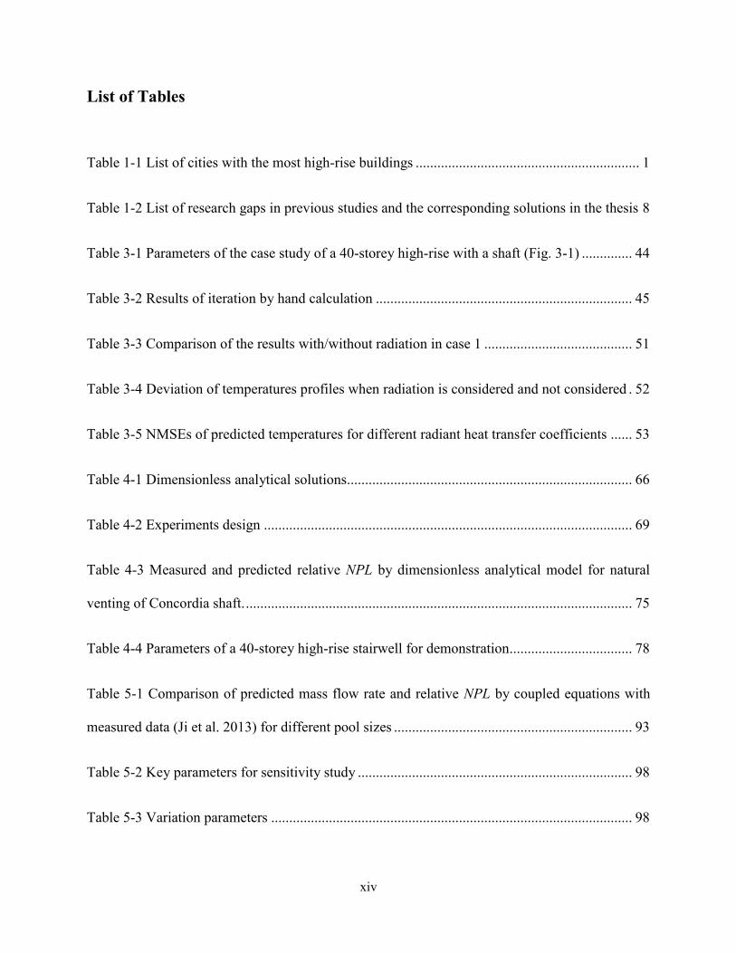
List of Tables

Table 1-1 List of cities with the most high-rise buildings .............................................................. 1

Table 1-2 List of research gaps in previous studies and the corresponding solutions in the thesis 8

Table 3-1 Parameters of the case study of a 40-storey high-rise with a shaft (Fig. 3-1) .............. 44

Table 3-2 Results of iteration by hand calculation ....................................................................... 45

Table 3-3 Comparison of the results with/without radiation in case 1 ......................................... 51

Table 3-4 Deviation of temperatures profiles when radiation is considered and not considered . 52

Table 3-5 NMSEs of predicted temperatures for different radiant heat transfer coefficients ...... 53

Table 4-1 Dimensionless analytical solutions............................................................................... 66

Table 4-2 Experiments design ...................................................................................................... 69

Table 4-3 Measured and predicted relative NPL by dimensionless analytical model for natural

venting of Concordia shaft. ........................................................................................................... 75

Table 4-4 Parameters of a 40-storey high-rise stairwell for demonstration .................................. 78

Table 5-1 Comparison of predicted mass flow rate and relative NPL by coupled equations with

measured data (Ji et al. 2013) for different pool sizes .................................................................. 93

Table 5-2 Key parameters for sensitivity study ............................................................................ 98

Table 5-3 Variation parameters .................................................................................................... 98

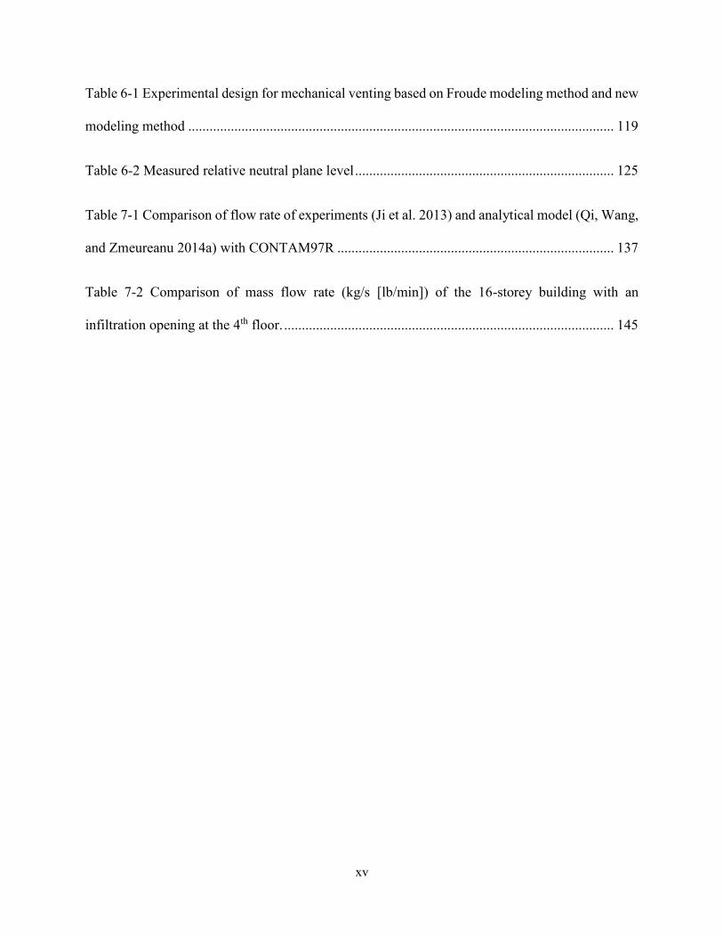
xv

Table 6-1 Experimental design for mechanical venting based on Froude modeling method and new

modeling method ........................................................................................................................ 119

Table 6-2 Measured relative neutral plane level ......................................................................... 125

Table 7-1 Comparison of flow rate of experiments (Ji et al. 2013) and analytical model (Qi, Wang,

and Zmeureanu 2014a) with CONTAM97R .............................................................................. 137

Table 7-2 Comparison of mass flow rate (kg/s [lb/min]) of the 16-storey building with an

infiltration opening at the 4th floor. ............................................................................................. 145

xvi

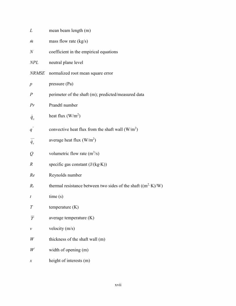
Nomenclature

a

ai

absorption coefficient; thermal diffusivity

emissivity weighting factor for the ith fictitious gray gas in the weighted sum of gray

gases model

A cross section area of the shaft (m2)

A* effective area of opening (m2)

Ah cross-section area (m2)

C pressure correction coefficient; coefficient in the empirical equations

Cd discharge coefficient

Cw coefficient for natural convection

Cp specific heat capacity of the smoke (J/(kg∙K))

D characteristic length (m)

E heat source (kW); heat release rate (kW)

H height of the shaft (m)

Hf height of the fire floor (m)

Hf/ height of opening (m)

Dh hydraulic diameter (m)

f dimensionless friction factor

Fr Froude mumber

h heat transfer coefficient (W/(m2∙K)); head loss caused by friction (m) ; height (m)

k conduction heat transfer coefficient of air (W/(m∙K))

ki absorption efficient of the ith gray gas in the weighted sum of gray gases model

l characteristic length (m)

xvii

L mean beam length (m)

ṁ mass flow rate (kg/s)

N coefficient in the empirical equations

NPL neutral plane level

NRMSE normalized root mean square error

p pressure (Pa)

P perimeter of the shaft (m); predicted/measured data

Pr Prandtl number

xq heat flux (W/m2)

q˝ convective heat flux from the shaft wall (W/m2)

xq average heat flux (W/m2)

Q volumetric flow rate (m3/s)

R specific gas constant (J/(kg∙K))

Re

Rt

Reynolds number

thermal resistance between two sides of the shaft ((m2·K)/W)

t time (s)

T temperature (K)

T

v

average temperature (K)

velocity (m/s)

W thickness of the shaft wall (m)

W/ width of opening (m)

x height of interests (m)

xviii

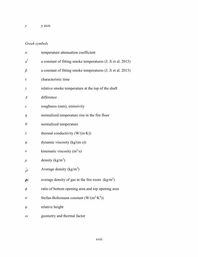
y y axis

Greek symbols

α temperature attenuation coefficient

a* a constant of fitting smoke temperatures (J. Ji et al. 2013)

β a constant of fitting smoke temperatures (J. Ji et al. 2013)

τ characteristic time

γ relative smoke temperature at the top of the shaft

Δ difference

ε roughness (mm); emissivity

η normalized temperature rise in the fire floor

θ normalized temperature

λ

μ

ν

thermal conductivity (W/(m∙K))

dynamic viscosity (kg/(m·s))

kinematic viscosity (m2/s)

ρ density (kg/m3)

Average density (kg/m3)

𝞺f/ average density of gas in the fire room (kg/m3)

ϕ ratio of bottom opening area and top opening area

σ Stefan-Boltzmann constant (W/(m2∙K4))

φ relative height

ω geometry and thermal factor

xix

Subscripts

0 ground level, the height of x = 0

1 expelling gas

a atmospheric

b bottom

c

CO2

convective

carbon dioxide

couple coupled equation

dy dynamic

e emittance

el elevation in the shaft

ek predicted results of empirical equation or Klote’s equation

f fire floor; full size

fr friction

g gas

H height of the shaft

i interior wall of the shaft; index of points of interests in the shaft; zone i; sub-section

i; inside of the shaft

in entry the shaft

j zone j

k wall k

l lower

m sub-scaled model scale

xx

n zone number

nf non-fire floor

np neutral pressure

o exterior wall of the shaft

out leave the shaft

r radiant

sh shaft

shl lower section of shaft below neutral plane level

shu upper section of shaft above neutral plane level

t top

u upper

w wall

xxi

Preface

This is a manuscript-based thesis, a collection of three published journal papers and two

manuscripts ready to be submitted. The five papers compose Chapter 3 ~ Chapter 7, and each

manuscript is an independent chapter.

For the purpose of easy reading, these five manuscripts are modified from the original ones. The

numbering of equations, tables, and figures includes the numbers of the chapters they belong to.

References of different chapters are combined at the end of the thesis.

1

Chapter 1 Introduction

According to the National Fire Protection Association (NFPA) 101 Life Safety Code (2012), a

high-rise building is defined as a building with the height of more than 23 m (roughly 7 stories).

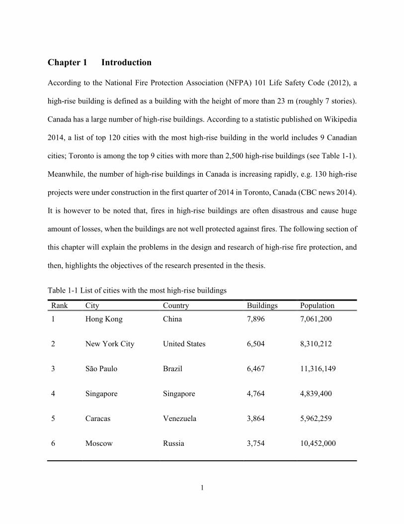
Canada has a large number of high-rise buildings. According to a statistic published on Wikipedia

2014, a list of top 120 cities with the most high-rise building in the world includes 9 Canadian

cities; Toronto is among the top 9 cities with more than 2,500 high-rise buildings (see Table 1-1).

Meanwhile, the number of high-rise buildings in Canada is increasing rapidly, e.g. 130 high-rise

projects were under construction in the first quarter of 2014 in Toronto, Canada (CBC news 2014).

It is however to be noted that, fires in high-rise buildings are often disastrous and cause huge

amount of losses, when the buildings are not well protected against fires. The following section of

this chapter will explain the problems in the design and research of high-rise fire protection, and

then, highlights the objectives of the research presented in the thesis.

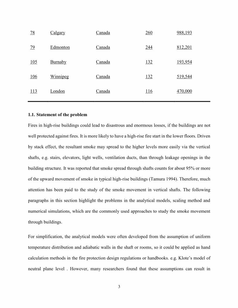
Table 1-1 List of cities with the most high-rise buildings

Rank City Country Buildings Population

1 Hong Kong China 7,896 7,061,200

2 New York City United States 6,504 8,310,212

3 São Paulo Brazil 6,467 11,316,149

4 Singapore Singapore 4,764 4,839,400

5 Caracas Venezuela 3,864 5,962,259

6 Moscow Russia 3,754 10,452,000

2

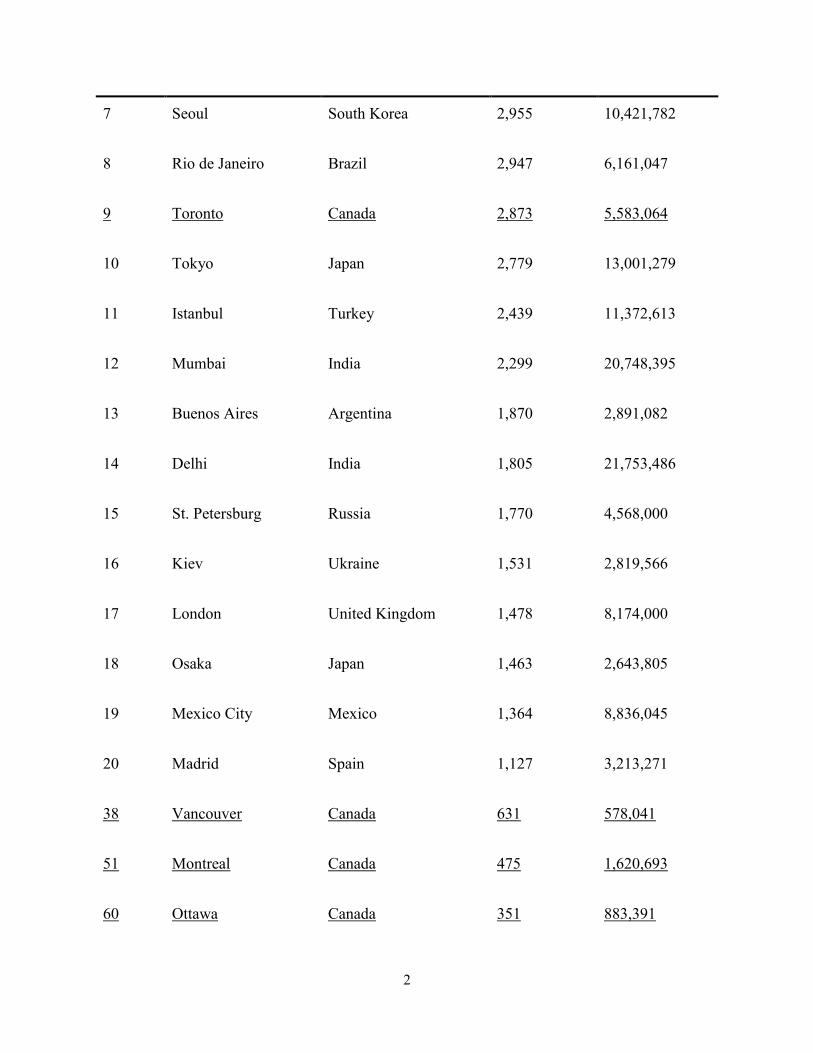
7 Seoul South Korea 2,955 10,421,782

8 Rio de Janeiro Brazil 2,947 6,161,047

9 Toronto Canada 2,873 5,583,064

10 Tokyo Japan 2,779 13,001,279

11 Istanbul Turkey 2,439 11,372,613

12 Mumbai India 2,299 20,748,395

13 Buenos Aires Argentina 1,870 2,891,082

14 Delhi India 1,805 21,753,486

15 St. Petersburg Russia 1,770 4,568,000

16 Kiev Ukraine 1,531 2,819,566

17 London United Kingdom 1,478 8,174,000

18 Osaka Japan 1,463 2,643,805

19 Mexico City Mexico 1,364 8,836,045

20 Madrid Spain 1,127 3,213,271

38 Vancouver Canada 631 578,041

51 Montreal Canada 475 1,620,693

60 Ottawa Canada 351 883,391

3

78 Calgary Canada 260 988,193

79 Edmonton Canada 244 812,201

105 Burnaby Canada 132 193,954

106 Winnipeg Canada 132 519,544

113 London Canada 116 470,000

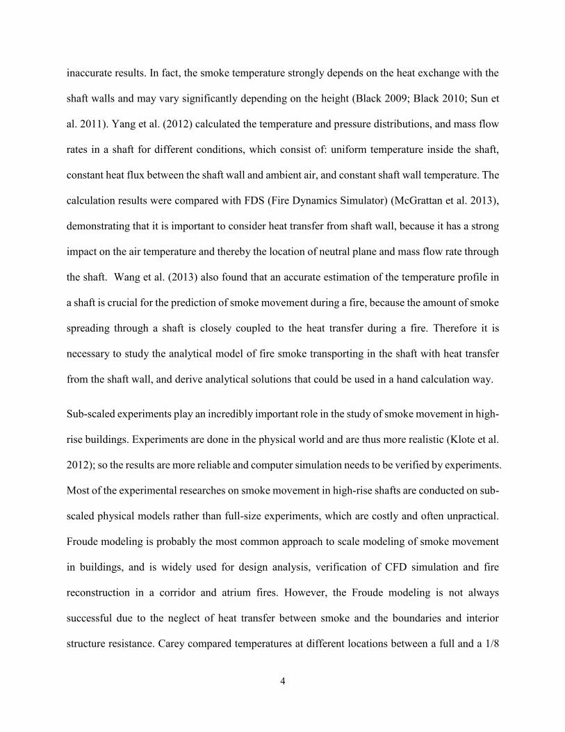
1.1. Statement of the problem

Fires in high-rise buildings could lead to disastrous and enormous losses, if the buildings are not

well protected against fires. It is more likely to have a high-rise fire start in the lower floors. Driven

by stack effect, the resultant smoke may spread to the higher levels more easily via the vertical

shafts, e.g. stairs, elevators, light wells, ventilation ducts, than through leakage openings in the

building structure. It was reported that smoke spread through shafts counts for about 95% or more

of the upward movement of smoke in typical high-rise buildings (Tamura 1994). Therefore, much

attention has been paid to the study of the smoke movement in vertical shafts. The following

paragraphs in this section highlight the problems in the analytical models, scaling method and

numerical simulations, which are the commonly used approaches to study the smoke movement

through buildings.

For simplification, the analytical models were often developed from the assumption of uniform

temperature distribution and adiabatic walls in the shaft or rooms, so it could be applied as hand

calculation methods in the fire protection design regulations or handbooks. e.g. Klote’s model of

neutral plane level . However, many researchers found that these assumptions can result in

4

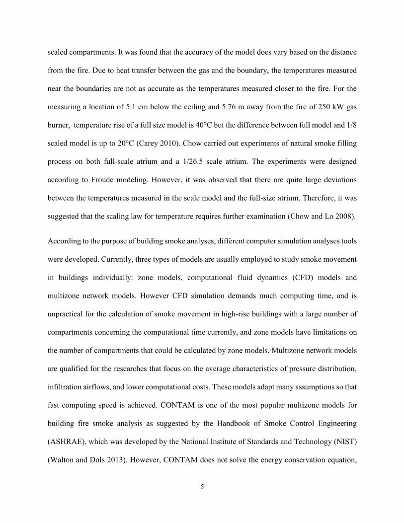
inaccurate results. In fact, the smoke temperature strongly depends on the heat exchange with the

shaft walls and may vary significantly depending on the height (Black 2009; Black 2010; Sun et

al. 2011). Yang et al. (2012) calculated the temperature and pressure distributions, and mass flow

rates in a shaft for different conditions, which consist of: uniform temperature inside the shaft,

constant heat flux between the shaft wall and ambient air, and constant shaft wall temperature. The

calculation results were compared with FDS (Fire Dynamics Simulator) (McGrattan et al. 2013),

demonstrating that it is important to consider heat transfer from shaft wall, because it has a strong

impact on the air temperature and thereby the location of neutral plane and mass flow rate through

the shaft. Wang et al. (2013) also found that an accurate estimation of the temperature profile in

a shaft is crucial for the prediction of smoke movement during a fire, because the amount of smoke

spreading through a shaft is closely coupled to the heat transfer during a fire. Therefore it is

necessary to study the analytical model of fire smoke transporting in the shaft with heat transfer

from the shaft wall, and derive analytical solutions that could be used in a hand calculation way.

Sub-scaled experiments play an incredibly important role in the study of smoke movement in high-

rise buildings. Experiments are done in the physical world and are thus more realistic (Klote et al.

2012); so the results are more reliable and computer simulation needs to be verified by experiments.

Most of the experimental researches on smoke movement in high-rise shafts are conducted on sub-

scaled physical models rather than full-size experiments, which are costly and often unpractical.

Froude modeling is probably the most common approach to scale modeling of smoke movement

in buildings, and is widely used for design analysis, verification of CFD simulation and fire

reconstruction in a corridor and atrium fires. However, the Froude modeling is not always

successful due to the neglect of heat transfer between smoke and the boundaries and interior

structure resistance. Carey compared temperatures at different locations between a full and a 1/8

5

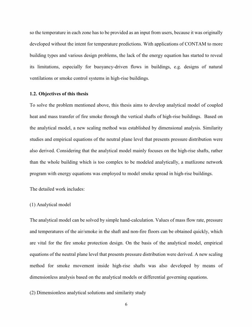
scaled compartments. It was found that the accuracy of the model does vary based on the distance

from the fire. Due to heat transfer between the gas and the boundary, the temperatures measured

near the boundaries are not as accurate as the temperatures measured closer to the fire. For the

measuring a location of 5.1 cm below the ceiling and 5.76 m away from the fire of 250 kW gas

burner, temperature rise of a full size model is 40°C but the difference between full model and 1/8

scaled model is up to 20°C (Carey 2010). Chow carried out experiments of natural smoke filling

process on both full-scale atrium and a 1/26.5 scale atrium. The experiments were designed

according to Froude modeling. However, it was observed that there are quite large deviations

between the temperatures measured in the scale model and the full-size atrium. Therefore, it was

suggested that the scaling law for temperature requires further examination (Chow and Lo 2008).

According to the purpose of building smoke analyses, different computer simulation analyses tools

were developed. Currently, three types of models are usually employed to study smoke movement

in buildings individually: zone models, computational fluid dynamics (CFD) models and

multizone network models. However CFD simulation demands much computing time, and is

unpractical for the calculation of smoke movement in high-rise buildings with a large number of

compartments concerning the computational time currently, and zone models have limitations on

the number of compartments that could be calculated by zone models. Multizone network models

are qualified for the researches that focus on the average characteristics of pressure distribution,

infiltration airflows, and lower computational costs. These models adapt many assumptions so that

fast computing speed is achieved. CONTAM is one of the most popular multizone models for

building fire smoke analysis as suggested by the Handbook of Smoke Control Engineering

(ASHRAE), which was developed by the National Institute of Standards and Technology (NIST)

(Walton and Dols 2013). However, CONTAM does not solve the energy conservation equation,

6

so the temperature in each zone has to be provided as an input from users, because it was originally

developed without the intent for temperature predictions. With applications of CONTAM to more

building types and various design problems, the lack of the energy equation has started to reveal

its limitations, especially for buoyancy-driven flows in buildings, e.g. designs of natural

ventilations or smoke control systems in high-rise buildings.

1.2. Objectives of this thesis

To solve the problem mentioned above, this thesis aims to develop analytical model of coupled

heat and mass transfer of fire smoke through the vertical shafts of high-rise buildings. Based on

the analytical model, a new scaling method was established by dimensional analysis. Similarity

studies and empirical equations of the neutral plane level that presents pressure distribution were

also derived. Considering that the analytical model mainly focuses on the high-rise shafts, rather

than the whole building which is too complex to be modeled analytically, a mutlizone network

program with energy equations was employed to model smoke spread in high-rise buildings.

The detailed work includes:

(1) Analytical model

The analytical model can be solved by simple hand-calculation. Values of mass flow rate, pressure

and temperatures of the air/smoke in the shaft and non-fire floors can be obtained quickly, which

are vital for the fire smoke protection design. On the basis of the analytical model, empirical

equations of the neutral plane level that presents pressure distribution were derived. A new scaling

method for smoke movement inside high-rise shafts was also developed by means of

dimensionless analysis based on the analytical models or differential governing equations.

(2) Dimensionless analytical solutions and similarity study

7

Studies on dimensionless analytical solutions and similarity were conducted based on the

analytical model, which provide a new scaling method to sub-scale smoke spreads in high-rise

shafts. The new scaling method was verified by experiments on different size and material shafts.

(3) Numerical modeling

A multizone network program with energy equations was employed to model the smoke movement

in high-rise buildings, including verification of energy equation in the multizone network model,

the application in high-rise buildings with and without infiltrations. Using a dimensionless number

that represents the temperature profile of smoke inside the shaft, the zoning method was optimized

for the numerical modeling.

1.3. Summary and thesis work introduction

This chapter introduces the research gaps in the study of high-rise fire protection and objectives of

this thesis. It was pointed out the vertical shafts in the high-rise buildings are the primary paths for

the fire smoke spread from lower part of the building to the higher part, and therefore is the study

subject in this thesis. Considering venting smoke is a sound alternative approach to protect smoke

spread to non-fire area, this research focused on the venting shaft, including natural venting and

mechanical venting. Problems in the previous researches were highlighted in Table 1-2.

To solve the problem of no heat transfer consideration in the analytical model, chapter 3 develops

an analytical model of the coupled heat and mass transfer of fire smoke through high-rise shafts.

Hand calculation method based on the analytical model is provided. Since the smoke movement

in shafts is a thermal couple problem, including mechanical energy equation, energy equation and

mass balance equation, iteration is needed in the hand calculation method. Because there is no

discretion in the three equations, it is easier to obtain convergent results by the hand calculation

8

than the method with discretion like CFD approach. Iteration numbers with different convergence

thresholds is also counted in the demo cases with different conditions to show this advantage.

Chapters 4 reports the development of dimensionless analytical solutions of smoke transport in

non-adiabatic high-rise shafts during fires, which could provide a fundamental understanding of

smoke transport physics.

Chapter 5 provides a method to develop an empirical equation to estimate the neutral plane level,

which distinguishes from previous study of neutral plane level with the consideration of

temperature variation with the height. The temperature variation is caused by heat exchange

between smoke and shaft walls, and therefore the smoke temperature inside the shaft is non-

uniform.

Chapters 6 presents studies on the similarity to identify groups of dimensionless numbers, and a

new scaling method to sub-scale high-rise shafts with the consideration of heat exchange between

smoke and shaft walls, and interior structure resistance.

Chapter 7 presents the approach to model smoke movement in high-rise buildings by a multizone

airflow and energy network program, CONTAM97R. Chapters 3 ~ 6 mainly focus on the vertical

shafts, which are the main paths for fire smoke spread in high-rise buildings. To expend the

calculation of the heat and mass transfer to the whole building, the multizone program and its

modeling method is presented in chapter 7.

Table 1-2 List of research gaps in previous studies and the corresponding solutions in the thesis

Research gaps in previous studies

Solutions in

this thesis

1 Lack of appropriate heat exchange consideration in analytical model Chapter 3

9

2

Lack of appropriate heat exchange and structure resistance consideration

in dimensionless analytical solutions and scaling law to design sub-scaled

model

Chapters 4 &6

3 Lack of heat exchange consideration in modeling of neutral plane level Chapter 5

4

Lack of modeling method of smoke spread in high-rise buildings by

multizone network program with energy model

Chapter 7

This study contributes to an improved analytical model in terms of dimensionless numbers, a new

scale modeling method, and a new airflow network zoning approach of high-rise shafts during

fires. Different from previous studies, the analytical model and new scale modeling method

consider heat transfer between the smoke and walls using thermal resistance between two sides of

the walls, as well as interior structure resistance; therefore they are more reasonable and accurate.

The new zoning approach for airflow network program considers temperature gradient so it can

achieve the same accurate with fewer zones compared with traditional zoning approach.

10

Chapter 2 Literature Review

2.1. Introduction

Fires in high-rise buildings often lead to huge amount of losses, when the fires are not well

controlled. It is reported that smoke movement in high-rise buildings kills approximately 75

percent of the fire victims in the United States. These fire deaths occur in areas remote from the

room where the fire originates and are due to the toxic effects of the smoke as it migrates

throughout a building (Gann et al. 1994; Beitel, Wakelin, and Beyler 2000). Caused by stack effect

and wind, smoke spreads beyond fire sources and to other spaces through multiple paths, such as

large space, floor piping hole, stairwells, elevator shafts and building envelopes (Su et al. 2011;

Poreh and Trebukov 2000; Tamura 1994). Smoke can also spread through building equipment,

such as the air-handling units and mechanical ventilation systems. Smoke movement throughout a

high-rise building is, therefore, an important issue with respect to the life safety of people who are

in a building when a fire occurs (Zhong et al. 2004; Hou et al. 2011; Luo et al. 2013). It also greatly

impacts the firefighting efforts both in search and rescue as well as the attack on the fire (Beitel,

Wakelin, and Beyler 2000).

Historically, a high-rise fire is found more likely to happen in the lower floors according to the

statistics (Hall 2011), resulting in more non-fire floors to be exposed to smoke. The Winecoff

Hotel fire at Atlanta, US (December 7, 1946) caused 119 deaths. The MGM Grand Hotel fire at

Las Vegas, NV (November 21, 1980) led to the deaths of 85 people and the injuries of 600 people

(Tamura 1994). It was reported that in the US between 2007 and 2011, 43% of fires in hotel

buildings originated below the 2nd floor, and 73% below the 6th floor, and 37% of fires in office

buildings originated below the 2nd floor, and 64% below the 7th floor. Driven by stack effect, the

resultant smoke from fires may spread to the higher levels more easily via the vertical shafts, e.g.

11

stairs, elevators, light wells, ventilation ducts, than through leakage openings in the building

structure. It was reported that smoke spread through shafts counts for about 95% or more of the

upward movement of smoke in typical high-rise buildings (Tamura 1994). Therefore, much

attention has been paid to the study of the smoke movement in vertical shafts, aiming to decrease

the smoke inside shafts (Harmathy 1998; Mercier and Jaluria 1999; Shi et al. 2014a).

To prevent smoke spread to higher levels, the pressurization systems have become a popular option

since the 1960s, which is intended to prevent the smoke leaking through closed doors into shafts

by injecting clean air into the shaft enclosure as the pressure in the shaft is greater than the adjacent

fire compartment (Lay 2014). However, the pressurization systems do not always work to prevent

smoke spreads through shafts, especially for the high-rise shafts due to stack effect and floor-to-

floor variations in flow resistance (Klote 2011). It was estimated that 35% of pressurization

systems might fail to function as intended (Lay 2014).

As an alternative solution, the idea of using ventilation to exhaust smoke from the fire floor or

keeping spaces tenable during high-rise fires attracts much attention. Many studies have been

conducted on the experiments, mathematical models and applications of smoke ventilation in

shafts. Ji and Shi did extensive experimental research to investigate transport characteristics of

thermal plume in the ventilated stairwell with two or multiple openings (Jie Ji et al. 2015; Li et al.

2014; Ji et al. 2013; Shi et al. 2014a). Harmthy proposed the Fire Drainage System to remove the

heat and induced convection flow from a fire through a series of shafts to reduce the spread of fire

from the region of fire source (Lay 2014; Harmathy and Oleszkiewicz 1987). Design principles of

this system were also introduced based on the assumption of constant gas temperature (Harmathy

and Oleszkiewicz 1987) and the heat transfer between the gas and shaft walls was not considered.

Similar to the Fire Drainage System, the Beetham Tower system was developed to use an air inlet

12

shaft to exhaust smoke from fire floor by stack effect but mechanical input was employed to

enhance the performance (Lay 2014). Klote studied the ventilation control of stairwells in tall

buildings by tenability analysis, computational fluid dynamics (CFD) and network modeling. It

was found that the stairwell smoke control by ventilation is feasible (Klote 2011). The elevator

hoistway shafts could also provide excellent paths to remove hot smoke out of the building, which

gains wide acceptance even in the absence of supporting research (Klote et al. 2012). The

International Building Code demands that hoistways of elevators and dumbwaiters penetrating

more than three stories shall be provided with a means for venting smoke and hot gases to the outer

air in case of a fire. Vents shall be located at the top of the hoistway and shall open either directly

to the outer air or through non-combustible ducts to the outer air (International Code Council 2007).

However, the hot smoke inside of the elevator hoistway shafts can also make the smoke flow from

the elevator shaft to the building, especially on the upper floors of buildings (Klote 2004).

Therefore, more attention needs to be paid to the elevator hoistway shafts design.

Analytical models, scaling method and numerical simulations are the commonly used approaches

to study the smoke movement through high-rise shafts during fires. Related previous researches

will be introduced in the following section in this chapter.

2.2. Analytical models

Hand calculation method that is based on the analytical models is essential to the fire smoke

protection design, because it is fast and simple to obtain important parameters for early stage

design. Generally, high-rise buildings could be simplified to three types of spaces, fire floor, non-

fire floor and shafts, each of which is calculated separately. As mentioned in section 2.1, the shafts

are very important for the fire smoke protection study, many researchers developed analytical

models of smoke movement in the shafts. Sections 2.2.1 and 2.2.2 will introduce the analytical

13

models developed by these studies based on uniform temperature and non-uniform temperature,

which do not consider heat transfer and consider heat transfer between smoke and shaft walls

respectively.

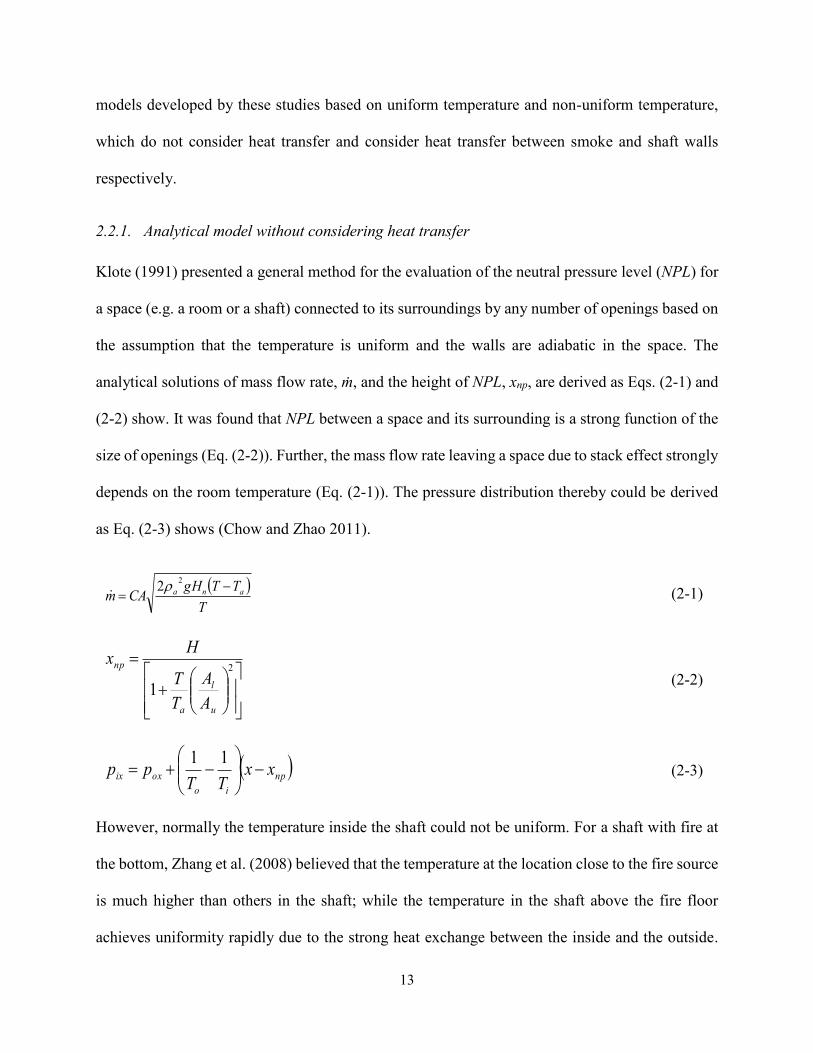
2.2.1. Analytical model without considering heat transfer

Klote (1991) presented a general method for the evaluation of the neutral pressure level (NPL) for

a space (e.g. a room or a shaft) connected to its surroundings by any number of openings based on

the assumption that the temperature is uniform and the walls are adiabatic in the space. The

analytical solutions of mass flow rate, ṁ, and the height of NPL, xnp, are derived as Eqs. (2-1) and

(2-2) show. It was found that NPL between a space and its surrounding is a strong function of the

size of openings (Eq. (2-2)). Further, the mass flow rate leaving a space due to stack effect strongly

depends on the room temperature (Eq. (2-1)). The pressure distribution thereby could be derived

as Eq. (2-3) shows (Chow and Zhao 2011).

T

TTgHCAm ana

22

(2-1)

2

1u

l

a

np

A

A

T

T

Hx

(2-2)

np

io

oxix xxTT

pp

11 (2-3)

However, normally the temperature inside the shaft could not be uniform. For a shaft with fire at

the bottom, Zhang et al. (2008) believed that the temperature at the location close to the fire source

is much higher than others in the shaft; while the temperature in the shaft above the fire floor

achieves uniformity rapidly due to the strong heat exchange between the inside and the outside.

14

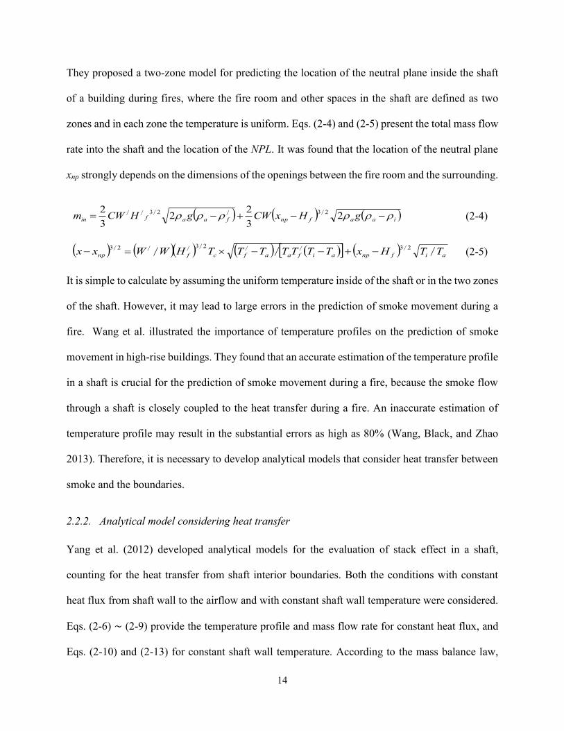
They proposed a two-zone model for predicting the location of the neutral plane inside the shaft

of a building during fires, where the fire room and other spaces in the shaft are defined as two

zones and in each zone the temperature is uniform. Eqs. (2-4) and (2-5) present the total mass flow

rate into the shaft and the location of the NPL. It was found that the location of the neutral plane

xnp strongly depends on the dimensions of the openings between the fire room and the surrounding.

iaafnpfaafin gHxCWgHCWm 23

22

3

2 2323 ///// (2-4)

aifnpaifaafcfnp TTHxTTTTTTTHWWxx ////////// 232323

(2-5)

It is simple to calculate by assuming the uniform temperature inside of the shaft or in the two zones

of the shaft. However, it may lead to large errors in the prediction of smoke movement during a

fire. Wang et al. illustrated the importance of temperature profiles on the prediction of smoke

movement in high-rise buildings. They found that an accurate estimation of the temperature profile

in a shaft is crucial for the prediction of smoke movement during a fire, because the smoke flow

through a shaft is closely coupled to the heat transfer during a fire. An inaccurate estimation of

temperature profile may result in the substantial errors as high as 80% (Wang, Black, and Zhao

2013). Therefore, it is necessary to develop analytical models that consider heat transfer between

smoke and the boundaries.

2.2.2. Analytical model considering heat transfer

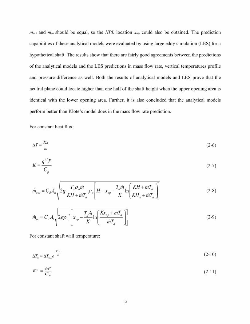
Yang et al. (2012) developed analytical models for the evaluation of stack effect in a shaft,

counting for the heat transfer from shaft interior boundaries. Both the conditions with constant

heat flux from shaft wall to the airflow and with constant shaft wall temperature were considered.

Eqs. (2-6) ~ (2-9) provide the temperature profile and mass flow rate for constant heat flux, and

Eqs. (2-10) and (2-13) for constant shaft wall temperature. According to the mass balance law,

15

ṁout and ṁin should be equal, so the NPL location xnp could also be obtained. The prediction

capabilities of these analytical models were evaluated by using large eddy simulation (LES) for a

hypothetical shaft. The results show that there are fairly good agreements between the predictions

of the analytical models and the LES predictions in mass flow rate, vertical temperatures profile

and pressure difference as well. Both the results of analytical models and LES prove that the

neutral plane could locate higher than one half of the shaft height when the upper opening area is

identical with the lower opening area. Further, it is also concluded that the analytical models

perform better than Klote’s model does in the mass flow rate prediction.

For constant heat flux:

m

KxT

(2-6)

pC

PqK

//

(2-7)

an

aanpa

a

aaudout

TmKH

TmKH

K

mTxH

TmKH

mTgACm

ln

2 (2-8)

a

anpanpaldin

Tm

TmKx

K

mTxgACm

ln

22 (2-9)

For constant shaft wall temperature:

m

xK

ww eTT

/

0,

(2-10)

pC

hPK /

(2-11)

16

mHK

ww

mHK

ww

w

anp

w

aamHK

ww

aaudout

neTT

eTT

TK

mTxH

T

T

eTT

TgACm

/

,.

/

,.

/

./

,.

/

/

/ ln0

0

0

12

(2-12)

a

mHK

ww

w

anp

w

aaldin

T

eTT

TK

mTx

T

TgACm

/

,.

/

.

/

ln02

12 (2-13)

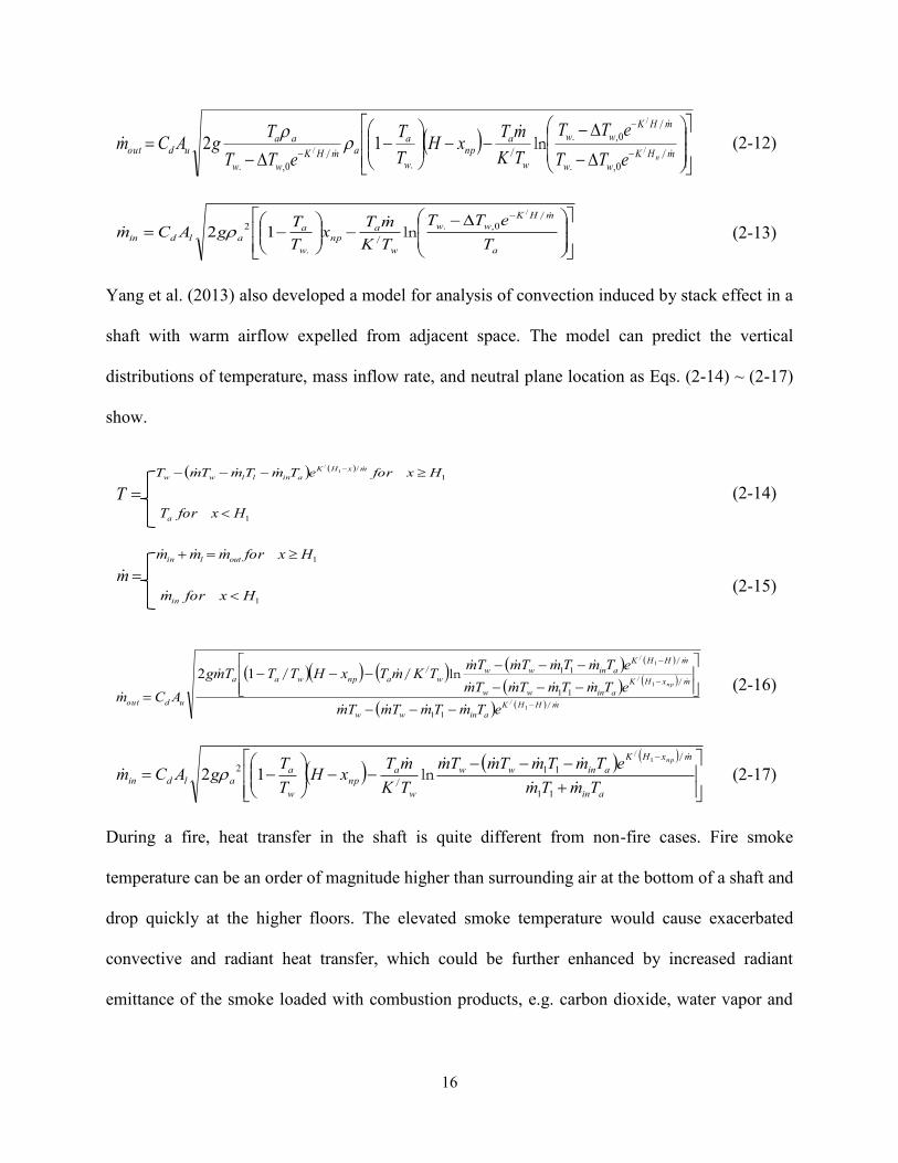
Yang et al. (2013) also developed a model for analysis of convection induced by stack effect in a

shaft with warm airflow expelled from adjacent space. The model can predict the vertical

distributions of temperature, mass inflow rate, and neutral plane location as Eqs. (2-14) ~ (2-17)

show.

1

/1/

HxforeTmTmTmTmxHK

ainllww

T

1HxforTa

(2-14)

1Hxformmm outlin

m

1Hxformin

(2-15)

mHHK

ainww

mxHK

ainww

mHHK

ainwwwanpwaa

udouteTmTmTmTm

eTmTmTmTm

eTmTmTmTmTKmTxHTTTmg

ACmnp

/

/

//

/

/

/

ln//

1

1

1

11

11

1112

(2-16)

ain

mxHK

ainww

w

anp

w

aaldin

TmTm

eTmTmTmTm

TK

mTxH

T

TgACm

np

11

1121

12

/

/

/

ln (2-17)

During a fire, heat transfer in the shaft is quite different from non-fire cases. Fire smoke

temperature can be an order of magnitude higher than surrounding air at the bottom of a shaft and

drop quickly at the higher floors. The elevated smoke temperature would cause exacerbated

convective and radiant heat transfer, which could be further enhanced by increased radiant

emittance of the smoke loaded with combustion products, e.g. carbon dioxide, water vapor and

17

soot. Meanwhile, both shaft surface temperature and heat flux would vary significantly with the

height of a shaft. Therefore, the previous studies of natural ventilation are not applicable.

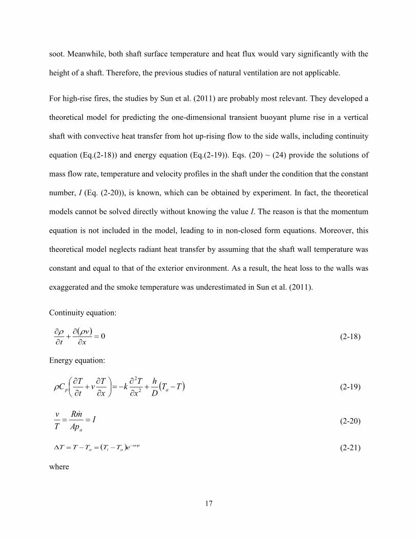
For high-rise fires, the studies by Sun et al. (2011) are probably most relevant. They developed a

theoretical model for predicting the one-dimensional transient buoyant plume rise in a vertical

shaft with convective heat transfer from hot up-rising flow to the side walls, including continuity

equation (Eq.(2-18)) and energy equation (Eq.(2-19)). Eqs. (20) ~ (24) provide the solutions of

mass flow rate, temperature and velocity profiles in the shaft under the condition that the constant

number, I (Eq. (2-20)), is known, which can be obtained by experiment. In fact, the theoretical

models cannot be solved directly without knowing the value I. The reason is that the momentum

equation is not included in the model, leading to in non-closed form equations. Moreover, this

theoretical model neglects radiant heat transfer by assuming that the shaft wall temperature was

constant and equal to that of the exterior environment. As a result, the heat loss to the walls was

exaggerated and the smoke temperature was underestimated in Sun et al. (2011).

Continuity equation:

0

x

v

t

(2-18)

Energy equation:

TTD

h

x

Tk

x

Tv

t

TC ap

2

2

(2-19)

IAp

mR

T

v

a

(2-20)

eTTTTT aia (2-21)

where

18

mDC

hHA

p

h

(2-22)

aoi

a

TeTTAp

mRv

(2-23)

H

x (2-24)

2.3. Scale modeling

Numerous studies have focused on the fire smoke movement inside high-rise large vertical spaces

by means of computer simulation and experiments, in which experiments play an incredible

important role. The experiment is done in the physical world and is more realistic (Klote et al.

2012); so the results are more reliable and computer simulation needs to be verified by it. Since

full-size fire experiments are costly and often unpractical to be conducted in buildings, most of the

experimental researches on smoke movement in high-rise buildings are conducted on sub-scaled

physical models. The sub-scaled modeling methods to simulate fire smoke spread in buildings

normally include the saltwater modeling and Froude modeling. The idea of saltwater modeling is

to substitute turbulent buoyant salt water moving in fresh water for turbulent buoyant hot gas

moving in cold gas (Steckler, Baum, and Quintiere 1986). The scale model is submerged in a tank

of fresh water and the inject salter simulates a heat source. Since the density of salt water is higher

than fresh water, the salt water tends to flow down whereas smoke tends to flow upward (Klote et

al. 2012). Steckler, Baum, and Quintiere (1986) used salt water modeling to study fire-induced

flows in multi-compartment structures. They developed the scaling laws relating salt water flows

and hot gas flows, based on which 1/20 scale salt water experiments were conducted to simulate

fire-induced flows in a single-story multi-room structure. The sub-scaled experimental results are

in good agreement with available full-scale results. The saltwater modeling was also applied to the

19

smoke filling visualization experiments on the atria and balcony spill plumes. The details can be

found in the work of Chow and Siu (1993) and Yii (1998), so they are not included here.

Froude modeling is probably the most common approach to scale modeling of smoke movement

in buildings, and is widely used for design analysis, verification of CFD simulation and fire

reconstruction. The Froude number, Fr, can be considered the ratio of inertial forces to buoyancy

gravity forces, which is shown in Eq. (2-25). The scaling relations are listed in Eqs. (2-26) to (2-

34).

gl

UFr

2

(2-25)

The scaling relations are:

f

mfm

l

lxx (2-26)

fm TT (2-27)

fm (2-28)

f

mfm

l

lvv (2-29)

25/

f

mfm

l

lQQ (2-30)

2/5

f

mfm

l

lmm (2-31)

f

mfm

l

ltt (2-32)

20

25/

f

mfm

l

lEE (2-33)

f

mfm

l

lpp (2-34)

Based on Froude modeling, Ding et al. (2004) developed a 1:25 scale model to validate CFD

simulations. Then, they carried out CFD simulations on a full size 8-storey building with a solar

chimney on top of the atrium to investigate the possibility of using the same system for natural

ventilation and smoke control in buildings. Froude modeling was also used to design experiments

on 1:10 physical scale model. The results of the experiments were employed to validate CFD

simulations. At last, both of the experimental and CFD results were used to investigate the hot

smoky gases entering an atrium from a fire within an adjacent compartment, (Harrison 2004).

Quintiere used a 1:7 geometric scale model in fire based on Froude modeling as evidence in civil

litigation case. It clarified the performance of a smoke control system which was operated in an

actual fire incident in a department store atrium. The scaled model results confirmed a design flaw

in the smoke control system. It was also found that the high velocity inlet air was shown to be

responsible for mixing and de-stratifying the hot smoke in the atrium and dispersing it throughout

the department store (Quintiere and Dillon 2008).

To study smoke movement inside high-rise buildings, 1:3 scaled building model was developed

by University of Science and Technology of China, which was designed using Froude modeling.

Extensive researches have been conducted on scaled building model. The topics include the

influence of the staircase ventilation state on the flow and heat transfer of the heated room on the

middle floor (Shi et al. 2014a), the effects of ventilation on the combustion characteristics in the

compartment connected to a stairwell (Ji et al. 2016).

21

However, due to the neglect of heat exchange between fire smoke and the boundaries, it was found

that sub-scaled experiments using Froude modeling may not obtain accurate temperature. Carey

compared temperatures at different locations between a full compartments and a 1:8 scaled

compartments designed based on Froude modeling. The accuracy of the model does vary based on

the distance from the fire. Due to heat transfer between the gas and the boundary, the temperatures

measured near the boundaries are not as accurate as the temperatures measured closer to the fire.

For the measuring location 5.1 cm below the ceiling and 5.76 m away from the fire of 250 kW gas

burner, temperature rise of full size model is 40°C but the difference between full model and 1:8

scaled model is up to 20°C (Allison C. Carey 2010). Chow carried out experiments of natural

smoke filling process on both full-scale atrium and a 1:26.5 scale atrium. The experiments were

designed according to Froude modeling. However, it was observed that there are quite large

deviations between the temperatures measured in the scale model and the full-size atrium.

Therefore, they suggested that the scaling law for temperature requires further examination (Chow

and Lo 2008). During a high-rise fire, fire smoke temperature can be an order of magnitude higher

than surrounding air at the bottom of large vertical spaces and drop quickly at the higher floor due

to the heat exchange between the fire smoke and the boundaries (Qi, Wang, and Zmeureanu 2014b).

It is necessary to consider the heat transfers when sub-scaling the large vertical spaces during fires.

2.4. Numerical modeling

Multizone network models are often used to calculate mechanically or naturally driven airflows

between different spaces (e.g. rooms) in a building, as well as between the building and the

outdoors (Wang and Chen 2008). Each space is defined as one zone with uniformly distributed air

parameters, e.g. air temperatures and species concentrations (Chen 2009), so that a whole-building

airflow analysis can be conducted within seconds. The simple and yet air quality (IAQ) analysis,

22

ventilation design, building safety and security analysis, e.g. fire smoke movement in buildings

(Wang, Black, and Zhao 2013). CONTAM is one of the most popular multizone models, which

was developed by the National Institute of Standards and Technology (NIST) (Walton and Dols

2013). It has been applied to many building types (Ng et al. 2012). Ng et al. (2012, 2013) used

CONTAM for the airflow and IAQ analysis in different DOE (the US Department of Energy)

reference buildings including restaurants, offices, schools, stores, hotels, hospitals and apartments.

Jo et al. (2007), Miller and Beasley (2009) and Miller (2011) conducted CONTAM simulations to

pressure distribution and smoke controls by the pressurization of the shafts in high-rise buildings.

However, CONTAM does not solve the energy conservation equation so the temperature in each

zone has to be provided as an input from users, because it was originally developed without the

intent for temperature predictions. With applications of CONTAM to more building types and

various design problems, the lack of the energy equation has started to reveal its limitations,

especially for buoyancy-driven flows in buildings, e.g. designs of natural ventilations or smoke

control systems in high-rise buildings. Wang, Black, and Zhao (2013) simulated the fire smoke

movement in a forty-storey building and found that the availability of temperature profile in the

shaft is the key to the accuracy of the prediction. The addition of the thermal analysis capability to

CONTAM thus becomes quite necessary.

There have been a few previous efforts to add the energy equation to CONTAM (Tang 2005; Tang

and Glicksman 2005; McDowell, Emmerich, Thornton, Walton 2003; Gu 2011), many of which

have not yet resulted in a final product. Among them, CONTAM97R (Axley 2001, Wang et al.

2012) is probably the most completed model, which was firstly developed in 1997 but not well

verified and/or validated so it was never released. Some previous studies tried to evaluate the

performance of CONTAM97R through experimental validations. Axley et al. (2012) compared

23

the measured airflow rates in a naturally ventilated building to the predictions, and found that the

difference could be over 25%. Such difference is also commonly seen in other experimental

validation studies with a discrepancy ranging between 25% and 50% (Mahdavi and Proglhof 2008,

Haghighat and Li 2004). Although experimental validation may be an effective way to prove the

validity of a numerical model, it is difficult to explain and isolate the causes for the discrepancies,

once observed, of the measurements and the predictions. Apparently, it is not reasonable to

attribute all the discrepancies to the computer model itself because there are many other

contributing factors, e.g. measurement uncertainties, user inputs, simplifications and assumptions

for the creation of the physical model of the problems. Therefore, experimental validation is

somehow limited during the evaluation of mathematical formulation and numerical discretization

of a computer model. In comparison, an analytical model provides a mathematical solution to the

same set of conservation equations formulated in a numerical model. Therefore, a verification

study based on analytical solutions is often conducted to evaluate the accuracy of a computer

model (Oberkampf and Trucano 2002, McDermott et al. 2010). The analytical solutions could also

help to identify causes of the discrepancies and to suggest necessary remedies.

24

Chapter 3 Analytical Model of Heat and Mass Transfer through Non-

adiabatic High-rise Shafts during fires

The contents of this chapter are published in “Dahai Qi, Liangzhu Wang, Radu Zmeureanu. 2014.

Analytical model of heat and mass transfer through non-adiabatic high-rise shafts during fires.

International Journal of Heat and Mass Transfer 72: 585-594”. The contents are slightly modified.

Abstract

Fire protection in high-rise buildings requires a good understanding of the physics of smoke spread

so that control measures can be properly undertaken. The problem is often complicated by the

coupled heat and mass transfer phenomena, especially when smoke spread through vertical shafts

far from a fire origin. Numerical analysis is often challenging due to limited computer resources

for such large structures. This study aims to develop an analytical model of the smoke movement

through a high-rise shaft under two ventilation conditions: the shaft with a given constant smoke

flow rate, and with the smoke purely driven by stack effect. A hand-calculation procedure is

proposed to obtain the solution to the analytical model, and demonstrated in a case of a 40-storey

building with a fire located at the 1st floor. The accuracy of the analytical model is confirmed by

comparisons to a numerical simulation and three experiments in the literature. It was found that

the calculated profiles of smoke temperatures and shaft wall temperatures depend on the

temperature attenuation coefficient a, a non-dimensional parameter associated with the

geometrical and thermal properties of the smoke and the shaft. The analytical solutions of the

smoke temperatures and smoke flow rates were plotted at different fire floor temperatures in non-

dimensional forms, which can be used for the design of shaft smoke controls. The effect of

radiation heat transfer on the calculation results was also discussed through a sensitivity study of

25

the analytical model. It was found that the calculated smoke and shaft wall temperatures seem not

quite sensitive to the radiation heat transfer in the case being studied.

3.1. Introduction

According to the National Fire Protection Association (NFPA) 101 Life Safety Code, a high-rise

building is defined as a building with the height more than 23 m (roughly 7 stories) (NFPA 101

2012). Fires in high-rise buildings are often disastrous and cause huge amount of losses, if the

buildings are not well protected against fires. The Winecoff Hotel fire at Atlanta, US (December

7, 1946) caused 119 deaths. The MGM Grand Hotel fire at Las Vegas, NV (November 21, 1980)

led to the deaths of 85 people and the injuries of 600 people (Tamura 1994). The terrorist attack

on the US World Trade Center on September 11, 2001 caused huge fires and subsequent building

collapse accounting for the deaths of 2,783 people. Between 2005 and 2009 in the North America

(Hall 2011), there were around 15,700 reported high-rise structure fires with the annually averaged

losses of 53 people, 546 injuries, and $235 million in direct property damage. Historically, a high-

rise fire is found more likely to happen in the lower floors according to the statistics (Hall 2011).

It was reported that in the US between 2007 and 2011, 43% of fires in hotel buildings originated

below the 2nd floor, and 73% below the 6th floor, and 37% of fires in office buildings originated

below the 2nd floor, and 64% below the 7th floor. Driven by stack effect, the resultant smoke from

fires may spread to the higher levels more easily via the vertical shafts, e.g. stairs, elevators, light

wells, ventilation ducts, than through leakage openings in building structure. Here, the stack effect

refers to buoyancy-driven airflows due to a difference of indoor/outdoor densities, which often

occur in building chimneys and/or flue gas stacks. It was reported that smoke spread through shafts

accounts for about 95% or more of the upward movement of smoke in typical high-rise buildings

26

(Tamura 1994). Therefore, much attention has been paid to the study of the smoke movement in

vertical shafts.

The risk of high-rise fire smoke spreads is closely related to the location of neutral pressure level

(NPL), where the shaft pressure is equal to that of the non-fire floor at the same height. Above a

NPL, the shaft pressure is higher than the non-fire floor so smoke would enter the non-fire floor if

there is a leakage (Klote 1991a). Klote presented a general method for the evaluation of the NPL

for a space (e.g. a room or a shaft) connected to its surroundings by any number of openings based

on the assumption that the temperature is uniform in the space (Klote 1991a). It was found that the

NPL between a space and its surrounding is a weak function of the room temperature but a strong

function of the size of openings. Further, the mass flow rate leaving a space due to stack effect

strongly depends on the room temperature. To predict the quantity of smoke entering a shaft,

Marshall (1986) developed an empirical equation based on the experiments in a 1/5 scale model

of a fire compartment with a corridor and a 5-storey open shaft. Xiao, Tu, and Yeoh (2008)

investigated numerically the effects of such dimensionless numbers as Grashof, Reynolds and Biot

numbers on smoke flow rate and temperature field. However, for simplification, these studies and

many of others often assumed adiabatic shaft walls and neglected heat transfer between smoke and

shaft boundaries. In fact, the smoke temperature strongly depends on the heat exchange with the

shaft walls and may vary significantly with the height (Black 2009; Sun et al. 2011). Wang, Black,

and Zhao (2013) also found that an accurate estimation of the temperature profile in a shaft is

crucial for the prediction of smoke movement during a fire, because the amount of smoke

spreading through a shaft is closely coupled to the heat transfer during a fire.

Numerical simulations and experimental studies are the commonly used methods to study the

coupled heat and mass transfer through building shafts. Popular numerical models used in the field

27

of building smoke control include but not limited to computational fluid dynamics (CFD), e.g. Fire

Dynamics Simulator (McGrattan et al. 2013) and ANSYS FLUENT, and simpler models such as

CONTAM (Dols and Polidoro 2015) and COSMO (i.e. COntrol of SMOke) (Black 2010). Black

studied the smoke movement and control by using COSMO (Black 2009). Peppes, Santamouris,

and Asimakopoulos (2001, 2002) conducted a series of experiments and CFD modeling studies,

showing that the smoke mass flow rate and the heat transfer rate are a function of the average

temperature difference between zones. However, both simulations and experiments are often

costly, time consuming, and experience demanding. It is often impractical to model a whole high-

rise building by CFD due to limited computer resources, or perform a costly full-scale field test.

Sub-scale experiments may be possible but it is not a trivial job to maintain the similarity of scaled

and full-size models. Therefore, designs of high-rise smoke controls often resort to hand

calculation methods based on analytical models.

In the literatures, analytical solutions to the coupled heat and mass transfer through a high-rise

shaft are relatively scarce. Some studies have touched upon the problem but were limited to non-

fire scenarios. Yam, Li, and Zheng (2008) provided an analytical solution to the coupled thermal

airflow problem in a naturally ventilated building. Yang et al. (2012, 2013) developed an analytical

model of a naturally-ventilated shaft by assuming either constant temperature or heat flux at the

interior surfaces of the shaft walls. It was found that the location of the neutral pressure level was

strongly associated with the heat transfer at the shaft wall surfaces. During a fire, heat transfer in

the shaft is quite different from non-fire cases. Fire smoke temperature can be an order of

magnitude higher than surrounding air at the bottom of a shaft and drop quickly at the higher floors.

The elevated smoke temperature would cause exacerbated convective and radiant heat transfer,

which could be further enhanced by increased radiant emittance of the smoke loaded with

28

combustion products, e.g. carbon dioxide, water vapor and soot. Meanwhile, both shaft surface

temperature and heat flux would vary significantly with the height of a shaft. Therefore, the

previous studies of natural ventilation are not applicable. For high-rise fires, the studies by Sun et

al. (2011) are probably most relevant. They developed an analytical model of the smoke plume

rise in a shaft by neglecting radiant heat transfer, and by assuming that the shaft wall temperature

was constant and equal to that of the exterior environment. As a result, the heat loss to the walls

was exaggerated and the smoke temperature was under estimated (Sun et al. 2011).

This paper aims to develop an analytical model of the coupled heat and mass transfer of fire smoke

through the vertical shafts of high-rise buildings. Analytical solutions are provided to the

temperature profiles of the smoke and the shaft wall surfaces (both interior and exterior), the

pressure distribution and the mass flow rate. We considered two scenarios of ventilation: a shaft

with a mechanical exhaust system at a given constant smoke flow rate, and the other with only

stack driven flow. For the case of mechanically ventilated shaft, the solution of the dimensionless

temperature profiles of smoke and wall temperatures are derived as a function of a so-called

temperature attenuation coefficient, which is a dimensionless number based on smoke mass flow

rate, thermal and geometric properties of the shaft. When the smoke through the shaft is only

driven by stack effect, a hand calculation method is reported for the prediction of pressure and

temperature profiles, and smoke mass flow rate. The accuracy of the analytical model is confirmed

by comparisons to a FDS simulation and three experiments in the literature. The method is then

demonstrated for a 40-story building with a fire located at the 1st floor, in which radiation is

neglected at first and its effect on the smoke movement is considered in a later section. This paper

also discusses the effect of radiation heat transfer on the calculation results in a sensitivity study

of the analytical model.

29

3.2. Building shaft with given smoke mass flow rate

For a mechanical smoke control system with a dedicated exhaust shaft (Klote et al. 2012), a ceiling

exhaust fan maintains a constant smoke mass flow rate through the shaft. One of the worst

scenarios is probably a fire located at the 1st floor and a bottom opening located at the ground level

so that all floors could be exposed to smoke as shown in Fig. 3-1. To formulate the analytical

model, we make the following assumptions:

Smoke movement in the shaft is one-dimensional at steady state.

The outdoor air temperature and the building temperature at non-fire floors are constant.

Specific heat capacity of the smoke, Cp, is constant.

The smoke is assumed to be incompressible and viscous but thermally expansible

satisfying the ideal gas law.

No smoke leaks through shaft wall Heat transfer coefficients (either due to convection or

radiation) are constant and do not vary along the height of the shaft.

The temperature of the fire floor is uniform and maintained at the fire smoke temperature

(Tamura 1994 and Black 2009).

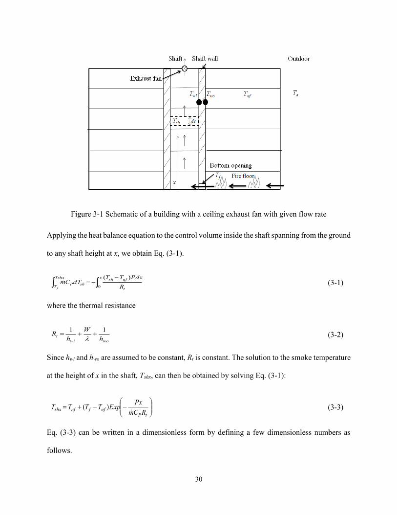
30

Figure 3-1 Schematic of a building with a ceiling exhaust fan with given flow rate

Applying the heat balance equation to the control volume inside the shaft spanning from the ground

to any shaft height at x, we obtain Eq. (3-1).

x

t

nfshTshx

TshP

R

PdxTTdTCm

f 0

)( (3-1)

where the thermal resistance

wowi

th

W

hR

11

(3-2)

Since hwi and hwo are assumed to be constant, Rt is constant. The solution to the smoke temperature

at the height of x in the shaft, Tshx, can then be obtained by solving Eq. (3-1):

tP

nffnfshxRCm

PxExpTTTT

)( (3-3)

Eq. (3-3) can be written in a dimensionless form by defining a few dimensionless numbers as

follows.

31

a) Dimensionless smoke temperature in the shaft:

nff

nfshx

shTT

TT

(3-4)

b) Relative height:

H

x (3-5)

c) Temperature attenuation coefficient:

tPRCm

PH

(3-6)

Eq. (3-3) can then be rewritten in the non-dimensional form:

Expsh (3-7)

The temperature attenuation coefficient, α, is a dimensionless number that depends on smoke mass

flow rate, thermal resistance between two sides of the shaft wall, and geometric features of the

shaft (height and circumference of the shaft cross sectional area). It considers the heat transfer on

both interior and exterior shaft walls, and solid wall conduction, which is different from the

attenuation coefficient in the literatures (Sun et al. 2011), which only considered the convection

on the interior shaft wall.

If we define the normalized temperature rise in the fire floor due to fire,

nf

nff

T

TT (3-8)

and the relative smoke temperature at the top of the shaft,

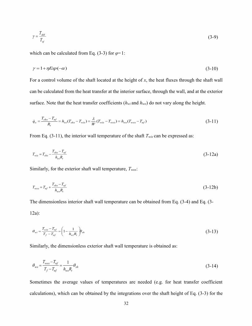
32

nf

shH

T

T (3-9)

which can be calculated from Eq. (3-3) for φ=1:

)(1 Exp (3-10)

For a control volume of the shaft located at the height of x, the heat fluxes through the shaft wall

can be calculated from the heat transfer at the interior surface, through the wall, and at the exterior

surface. Note that the heat transfer coefficients (hwi and hwo) do not vary along the height.

)()()( nfwoxwowoxwixwixshxwi

t

nfshx

x TThTTW

TThR

TTq

(3-11)

From Eq. (3-11), the interior wall temperature of the shaft Twix can be expressed as:

twi

nfshx

shxwixRh

TTTT

(3-12a)

Similarly, for the exterior shaft wall temperature, Twox:

two

nfshx

nfwoxRh

TTTT

(3-12b)

The dimensionless interior shaft wall temperature can be obtained from Eq. (3-4) and Eq. (3-

12a):

sh

twinff

nfwix

wiRhTT

TT

11 (3-13)

Similarly, the dimensionless exterior shaft wall temperature is obtained as:

sh

twonff

nfwox

woRhTT

TT

1

(3-14)

Sometimes the average values of temperatures are needed (e.g. for heat transfer coefficient

calculations), which can be obtained by the integrations over the shaft height of Eq. (3-3) for the

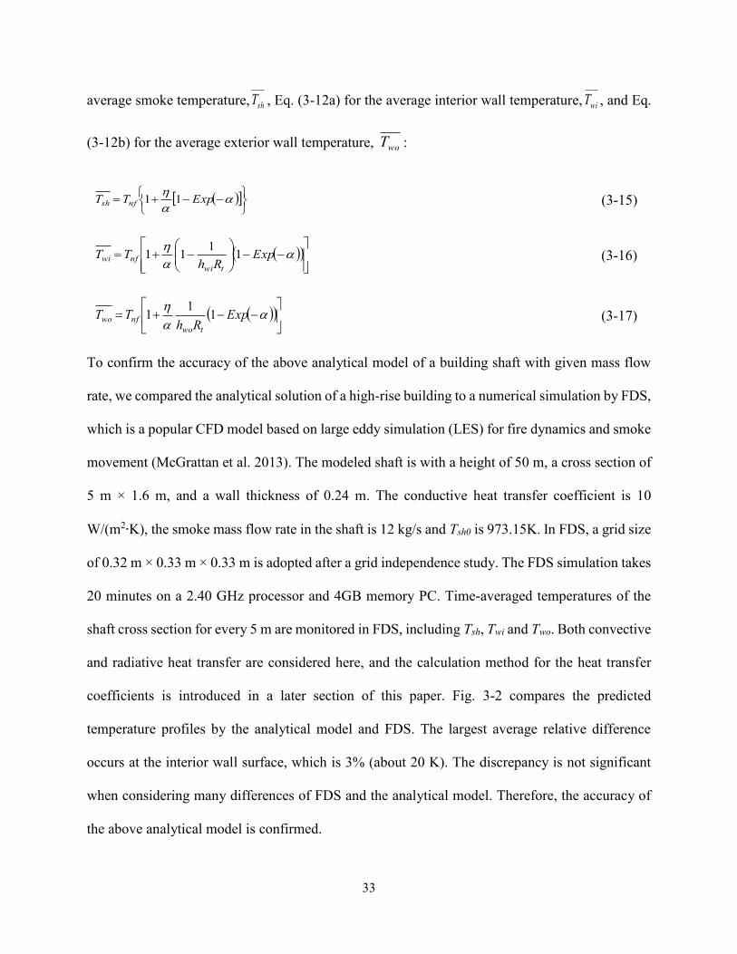
33

average smoke temperature, shT , Eq. (3-12a) for the average interior wall temperature, wiT , and Eq.

(3-12b) for the average exterior wall temperature, woT :

ExpTT nfsh 11 (3-15)

Exp

RhTT

twi

nfwi 11

11 (3-16)

Exp

RhTT

two

nfwo 11

1 (3-17)

To confirm the accuracy of the above analytical model of a building shaft with given mass flow

rate, we compared the analytical solution of a high-rise building to a numerical simulation by FDS,

which is a popular CFD model based on large eddy simulation (LES) for fire dynamics and smoke

movement (McGrattan et al. 2013). The modeled shaft is with a height of 50 m, a cross section of

5 m × 1.6 m, and a wall thickness of 0.24 m. The conductive heat transfer coefficient is 10

W/(m2∙K), the smoke mass flow rate in the shaft is 12 kg/s and Tsh0 is 973.15K. In FDS, a grid size

of 0.32 m × 0.33 m × 0.33 m is adopted after a grid independence study. The FDS simulation takes

20 minutes on a 2.40 GHz processor and 4GB memory PC. Time-averaged temperatures of the

shaft cross section for every 5 m are monitored in FDS, including Tsh, Twi and Two. Both convective

and radiative heat transfer are considered here, and the calculation method for the heat transfer

coefficients is introduced in a later section of this paper. Fig. 3-2 compares the predicted

temperature profiles by the analytical model and FDS. The largest average relative difference

occurs at the interior wall surface, which is 3% (about 20 K). The discrepancy is not significant

when considering many differences of FDS and the analytical model. Therefore, the accuracy of

the above analytical model is confirmed.

34

Figure 3-2 Comparison of the calculated temperatures by the analytical model and FDS

Meanwhile, a few major conclusions can be made from the analytical model. For a given smoke

mass flow through a shaft, Eq. (3-7) illustrates that the smoke temperature is an exponential

function of the product of dimensionless height and temperature attenuation coefficient. The

exponential temperature profile is consistent to the predictions by some numerical models in the

literatures. Wang, Black, and Zhao (2013) modeled a forty-storey building with four stairwell

shafts by COSMO and found that the shaft temperature cannot be simplified as a linear profile but

in fact follows a curve similar to an exponential distribution. It also shows that the temperature

profile can become linear for small values of α by plotting Eq. (3-7) as shown in Fig. 3-3. When α

is small enough, e.g. less than 0.3, the smoke temperature profile approaches linear. When α is

large enough (e.g. α ≥ 100), the entire shaft temperature is almost uniform and close to the non-

fire floor temperature, Tnf, and as well the temperature only decreases within the height of 0.05H.

This can be explained by that a large α value could indicate a small smoke mass flow or low

thermal resistances of the walls so the effect of the fire smoke on the shaft temperature becomes

35

minimal. When α is very small (e.g. α ≤ 0.05), the smoke temperature also becomes uniform but

close to fire floor temperature, Tf, due to the domination of a high smoke flow in the shaft or a high

thermal insulation of the shaft walls. Therefore, Eq. (3-7) and its illustration in Fig. 3-3 provide

the quantitative description of the transition of the shaft smoke temperature with the physical and

geometrical properties of the shaft. One immediate application is the use of the temperature profile

as the initial guess of the smoke/air temperatures in a shaft in a fire computer model or in a

computer model of naturally ventilated buildings. Moreover, both interior and exterior shaft wall

temperatures are a function of α as shown by Eqs. (3-13) and (3-14), which can also be used as

initial guesses of boundary conditions in fire computer models.

Figure 3-3 Dimensionless smoke temperature profile

The temperature at the top of the shaft, TshH, is important for the selection of smoke exhaust fan

installed at the shaft top (Klote et al. 2012) for the consideration of the safe operation of the fan.

The EN 12101-3 standard of the European Committee for Standardization (EN 12101-3 Standard

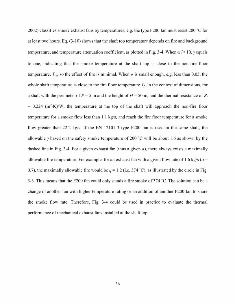
36

2002) classifies smoke exhaust fans by temperatures, e.g. the type F200 fan must resist 200 ˚C for

at least two hours. Eq. (3-10) shows that the shaft top temperature depends on fire and background

temperature, and temperature attenuation coefficient, as plotted in Fig. 3-4. When α ≥ 10, γ equals

to one, indicating that the smoke temperature at the shaft top is close to the non-fire floor

temperature, Tnf, so the effect of fire is minimal. When α is small enough, e.g. less than 0.05, the

whole shaft temperature is close to the fire floor temperature Tf. In the context of dimensions, for

a shaft with the perimeter of P = 5 m and the height of H = 50 m, and the thermal resistance of Rt

= 0.224 (m2∙K)/W, the temperature at the top of the shaft will approach the non-fire floor

temperature for a smoke flow less than 1.1 kg/s, and reach the fire floor temperature for a smoke

flow greater than 22.2 kg/s. If the EN 12101-3 type F200 fan is used in the same shaft, the

allowable γ based on the safety smoke temperature of 200 ˚C will be about 1.6 as shown by the

dashed line in Fig. 3-4. For a given exhaust fan (thus a given α), there always exists a maximally

allowable fire temperature. For example, for an exhaust fan with a given flow rate of 1.6 kg/s (α =

0.7), the maximally allowable fire would be η = 1.2 (i.e. 374 ˚C), as illustrated by the circle in Fig.

3-3. This means that the F200 fan could only stands a fire smoke of 374 ˚C. The solution can be a

change of another fan with higher temperature rating or an addition of another F200 fan to share

the smoke flow rate. Therefore, Fig. 3-4 could be used in practice to evaluate the thermal

performance of mechanical exhaust fans installed at the shaft top.

37

Figure 3-4 Relative smoke temperature at the top of the shaft

3.3. Building shaft with smoke driven by stack effect only

If a shaft has no mechanical exhaust system, the smoke flow in the shaft is only driven by stack

effect as shown in Fig. 3-1, where the exhaust fan is replaced by an opening at the top. The smoke

movement driven only by stack effect is also of particular interests because it helps to understand

the transport route of the smoke and aids the deployment of active smoke control measures. In a

stack-driven flow, the solution to temperature and pressure profiles, as well as mass flow rate

through a shaft is a coupled problem of heat and mass transfer. The calculation of the temperature

profiles is based on the same equations, Eqs. (3-7), (3-13) and (3-14), in the previous section. Here,

we focus on how to obtain the pressure profile and the resultant smoke mass flow rate in the shaft.

For incompressible and viscous flow at steady state, the mechanical energy equation (Munson et

al. 2009) for the control volume in Fig. 3-1 can be obtained.

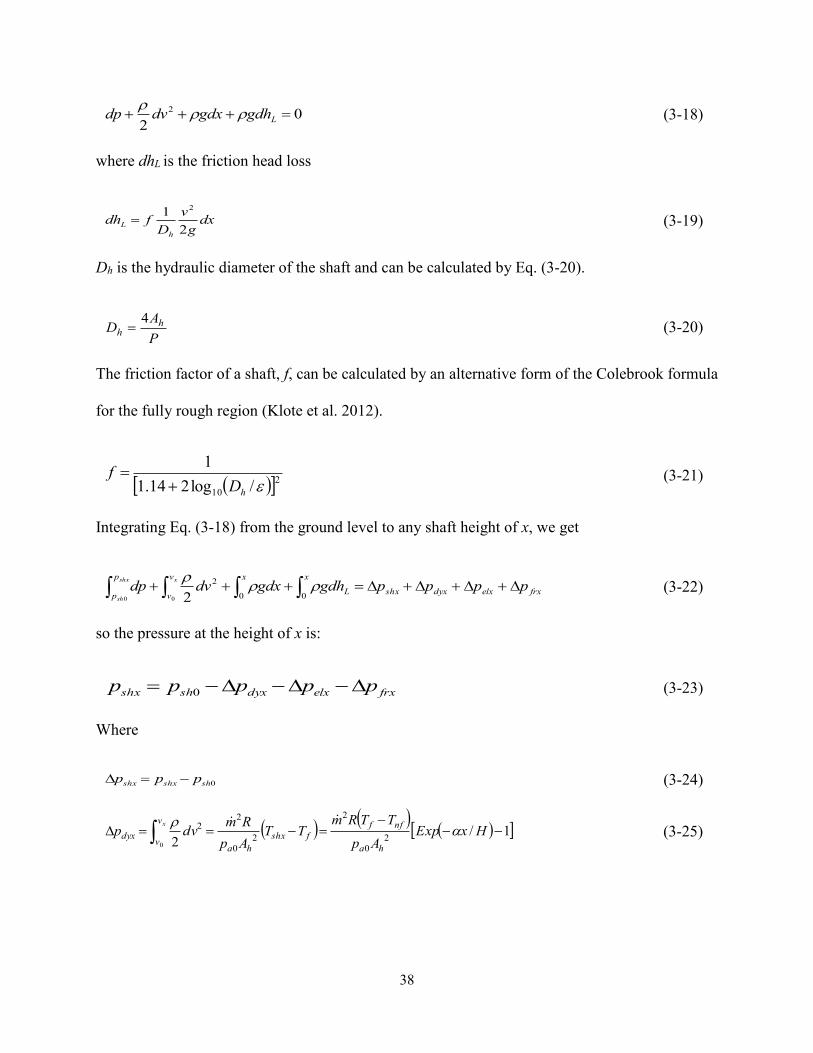
38

02

2 Lgdhgdxdvdp

(3-18)

where dhL is the friction head loss

dxg

v

Dfdh

h

L2

1 2

(3-19)

Dh is the hydraulic diameter of the shaft and can be calculated by Eq. (3-20).

P

AD h

h

4 (3-20)

The friction factor of a shaft, f, can be calculated by an alternative form of the Colebrook formula

for the fully rough region (Klote et al. 2012).

210 /log214.1

1

hDf

(3-21)

Integrating Eq. (3-18) from the ground level to any shaft height of x, we get

frxelxdyxshx

x

L

xv

v

p

pppppgdhgdxdvdp

xshx

sh

00

2

00 2

(3-22)

so the pressure at the height of x is:

frxelxdyxshshx ppppp 0 (3-23)

Where

0shshxshx ppp (3-24)

1/2 2

0

2

20

22

0

HxExpAp

TTRmTT

Ap

Rmdvp

ha

nff

fshx

ha

v

vdyx

x

(3-25)

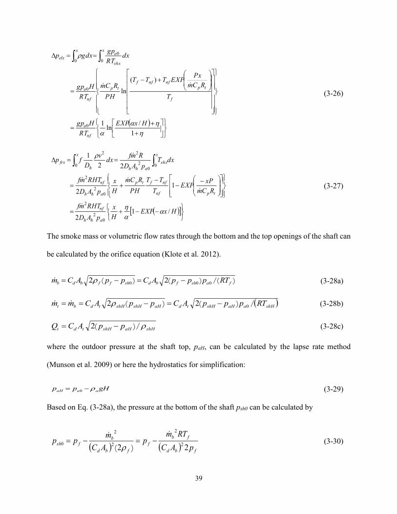
39

1

/ln

1

)(

ln

0

0

0

0

0

HxEXP

RT

Hgp

T

RCm

PxEXPTTT

PH

RCm

RT

Hgp

dxRT

gpgdxp

nf

a

f

tp

nfnff

tp

nf

a

x

shx

ax

elx

(3-26)

HxEXPH

x

pAD

RHTmf

RCm

xPEXP

T

TT

PH

RCm

H

x

pAD

RHTmf

dxTpAD

Rmfdx

v

Dfp

ahh

nf

tpnf

nfftp

ahh

nf

x

shx

ahh

x

h

frx

/12

12

22

1

02

2

02

2

00

2

2

0

2

(3-27)

The smoke mass or volumetric flow rates through the bottom and the top openings of the shaft can

be calculated by the orifice equation (Klote et al. 2012).

)/()()( fashfbdshffbdb RTpppACppACm 000 22 (3-28a)

shHaaHshHtdaHshHshHtdbt RTpppACppACmm /)()( 022 (3-28b)

shHaHshHtdt ppACQ /)( 2 (3-28c)

where the outdoor pressure at the shaft top, paH, can be calculated by the lapse rate method

(Munson et al. 2009) or here the hydrostatics for simplification:

gHpp aaaH 0 (3-29)

Based on Eq. (3-28a), the pressure at the bottom of the shaft psh0 can be calculated by

fbd

fb

f

fbd

bfsh

pAC

RTmp

AC

mpp

222

2

2

2

0

)( (3-30)

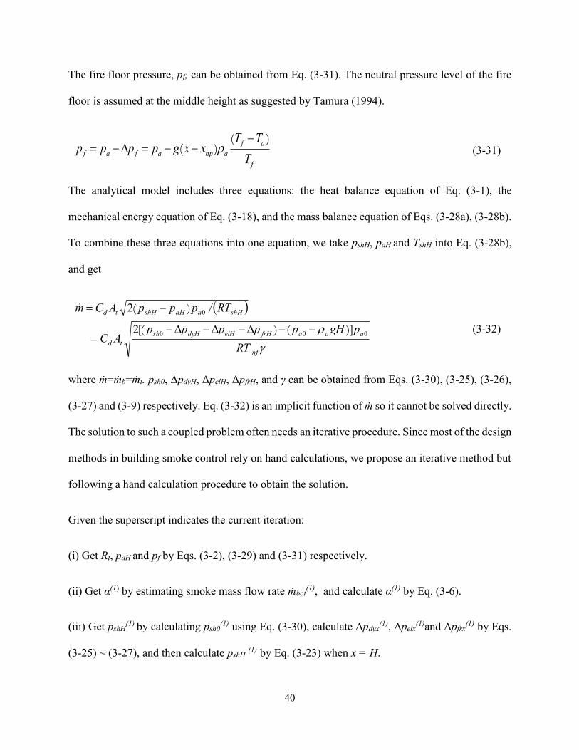
40

The fire floor pressure, pf, can be obtained from Eq. (3-31). The neutral pressure level of the fire

floor is assumed at the middle height as suggested by Tamura (1994).

f

af

anpafafT

TTxxgpppp

)()(

(3-31)

The analytical model includes three equations: the heat balance equation of Eq. (3-1), the

mechanical energy equation of Eq. (3-18), and the mass balance equation of Eqs. (3-28a), (3-28b).

To combine these three equations into one equation, we take pshH, paH and TshH into Eq. (3-28b),

and get

nf

aaafrHelHdyHsh

td

shHaaHshHtd

RT

pgHpppppAC

RTpppACm

000

0

2

2

)]()[(

/)(

(3-32)

where ṁ=ṁb=ṁt. psh0, ΔpdyH, ΔpelH, ΔpfrH, and γ can be obtained from Eqs. (3-30), (3-25), (3-26),

(3-27) and (3-9) respectively. Eq. (3-32) is an implicit function of ṁ so it cannot be solved directly.

The solution to such a coupled problem often needs an iterative procedure. Since most of the design

methods in building smoke control rely on hand calculations, we propose an iterative method but

following a hand calculation procedure to obtain the solution.

Given the superscript indicates the current iteration:

(i) Get Rt, paH and pf by Eqs. (3-2), (3-29) and (3-31) respectively.

(ii) Get α(1) by estimating smoke mass flow rate ṁbot(1), and calculate α(1) by Eq. (3-6).

(iii) Get pshH(1) by calculating psh0

(1) using Eq. (3-30), calculate Δpdyx(1), Δpelx

(1)and Δpfrx(1) by Eqs.

(3-25) ~ (3-27), and then calculate pshH (1) by Eq. (3-23) when x = H.

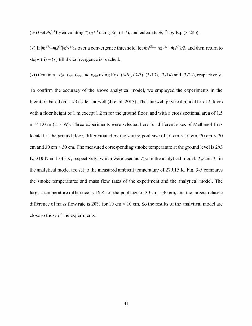
41

(iv) Get ṁt(1) by calculating TshH (1) using Eq. (3-7), and calculate ṁt

(1) by Eq. (3-28b).

(v) If |ṁt(1)–ṁb

(1)|/ṁt(1) is over a convergence threshold, let ṁb

(2)= (ṁt(1)+ṁb

(1))/2, and then return to

steps (ii) – (v) till the convergence is reached.

(vi) Obtain α, θsh, θwi, θwo and pshx using Eqs. (3-6), (3-7), (3-13), (3-14) and (3-23), respectively.

To confirm the accuracy of the above analytical model, we employed the experiments in the

literature based on a 1/3 scale stairwell (Ji et al. 2013). The stairwell physical model has 12 floors

with a floor height of 1 m except 1.2 m for the ground floor, and with a cross sectional area of 1.5

m × 1.0 m (L × W). Three experiments were selected here for different sizes of Methanol fires

located at the ground floor, differentiated by the square pool size of 10 cm × 10 cm, 20 cm × 20

cm and 30 cm × 30 cm. The measured corresponding smoke temperature at the ground level is 293

K, 310 K and 346 K, respectively, which were used as Tsh0 in the analytical model. Tnf and Ta in

the analytical model are set to the measured ambient temperature of 279.15 K. Fig. 3-5 compares

the smoke temperatures and mass flow rates of the experiment and the analytical model. The

largest temperature difference is 16 K for the pool size of 30 cm × 30 cm, and the largest relative

difference of mass flow rate is 20% for 10 cm × 10 cm. So the results of the analytical model are

close to those of the experiments.

42

Figure 3-5 Comparison of smoke temperatures (lines) and mass flow rates (table) of the

experiment (Ji et al. 2013) the analytical model

The above procedure of hand calculation method is demonstrated by a case study of a 40-storey

concrete building with a shaft, which is similar to the building in Fig. 3-1 but without the exhaust

fan. In the building, all the non-fire floors are assumed to have openings uniformly distributed

above and below the mid-height without significant internal resistance as suggested by the

literature (ASHRAE 2009). Therefore the pressures of the non-fire floors thus distribute

hydrostatically as calculated by Eq. (3-33), which is not used to develop analytical model but

calculate the non-fire floor pressure and study the NPL of the shaft in this case. Stronger stack

effect in the shaft can be created by lower outdoor temperature. To model one of the worst

scenarios of smoke spreads, the outdoor temperature is chose as 253.15 K, representing a winter

condition. The analytical model can be applied to summer conditions, which were not included

here due to page limit. Table 3-1 lists all the parameters for the calculation of the case study.

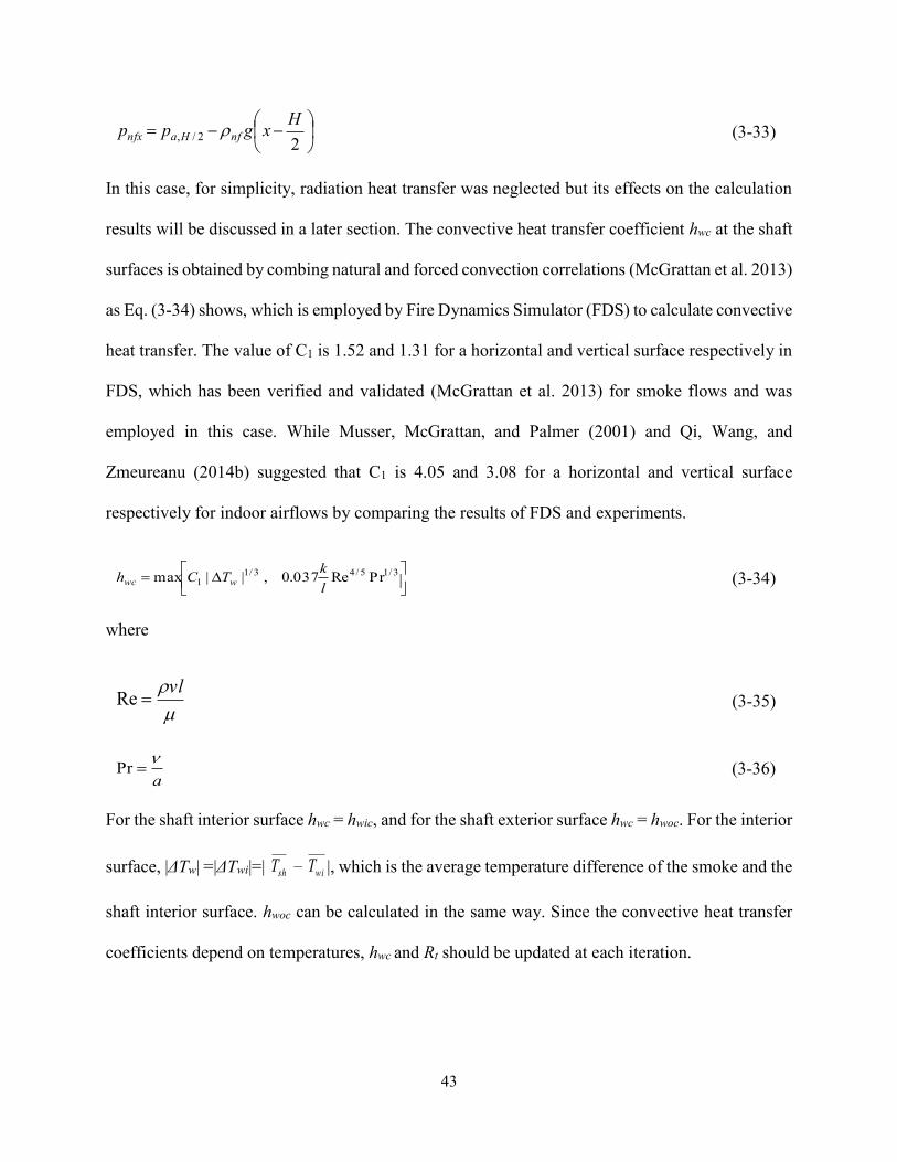
43

22/,

Hxgpp nfHanfx (3-33)

In this case, for simplicity, radiation heat transfer was neglected but its effects on the calculation

results will be discussed in a later section. The convective heat transfer coefficient hwc at the shaft

surfaces is obtained by combing natural and forced convection correlations (McGrattan et al. 2013)

as Eq. (3-34) shows, which is employed by Fire Dynamics Simulator (FDS) to calculate convective

heat transfer. The value of C1 is 1.52 and 1.31 for a horizontal and vertical surface respectively in

FDS, which has been verified and validated (McGrattan et al. 2013) for smoke flows and was

employed in this case. While Musser, McGrattan, and Palmer (2001) and Qi, Wang, and

Zmeureanu (2014b) suggested that C1 is 4.05 and 3.08 for a horizontal and vertical surface

respectively for indoor airflows by comparing the results of FDS and experiments.

3/15/43/1

1 PrRe037.0,||maxl

kTCh wwc

(3-34)

where

vlRe (3-35)

a

Pr (3-36)

For the shaft interior surface hwc = hwic, and for the shaft exterior surface hwc = hwoc. For the interior

surface, |ΔTw| =|ΔTwi|=| shT − wiT |, which is the average temperature difference of the smoke and the

shaft interior surface. hwoc can be calculated in the same way. Since the convective heat transfer

coefficients depend on temperatures, hwc and Rt should be updated at each iteration.

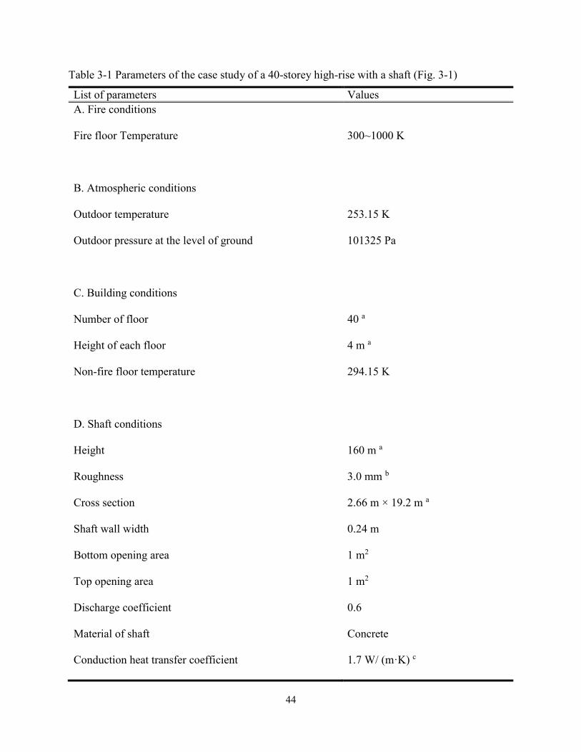
44

Table 3-1 Parameters of the case study of a 40-storey high-rise with a shaft (Fig. 3-1)

List of parameters Values

A. Fire conditions

Fire floor Temperature 300~1000 K

B. Atmospheric conditions

Outdoor temperature 253.15 K

Outdoor pressure at the level of ground 101325 Pa

C. Building conditions

Number of floor 40 a

Height of each floor 4 m a

Non-fire floor temperature 294.15 K

D. Shaft conditions

Height 160 m a

Roughness 3.0 mm b

Cross section 2.66 m × 19.2 m a

Shaft wall width 0.24 m

Bottom opening area 1 m2

Top opening area 1 m2

Discharge coefficient 0.6

Material of shaft Concrete

Conduction heat transfer coefficient 1.7 W/ (m·K) c

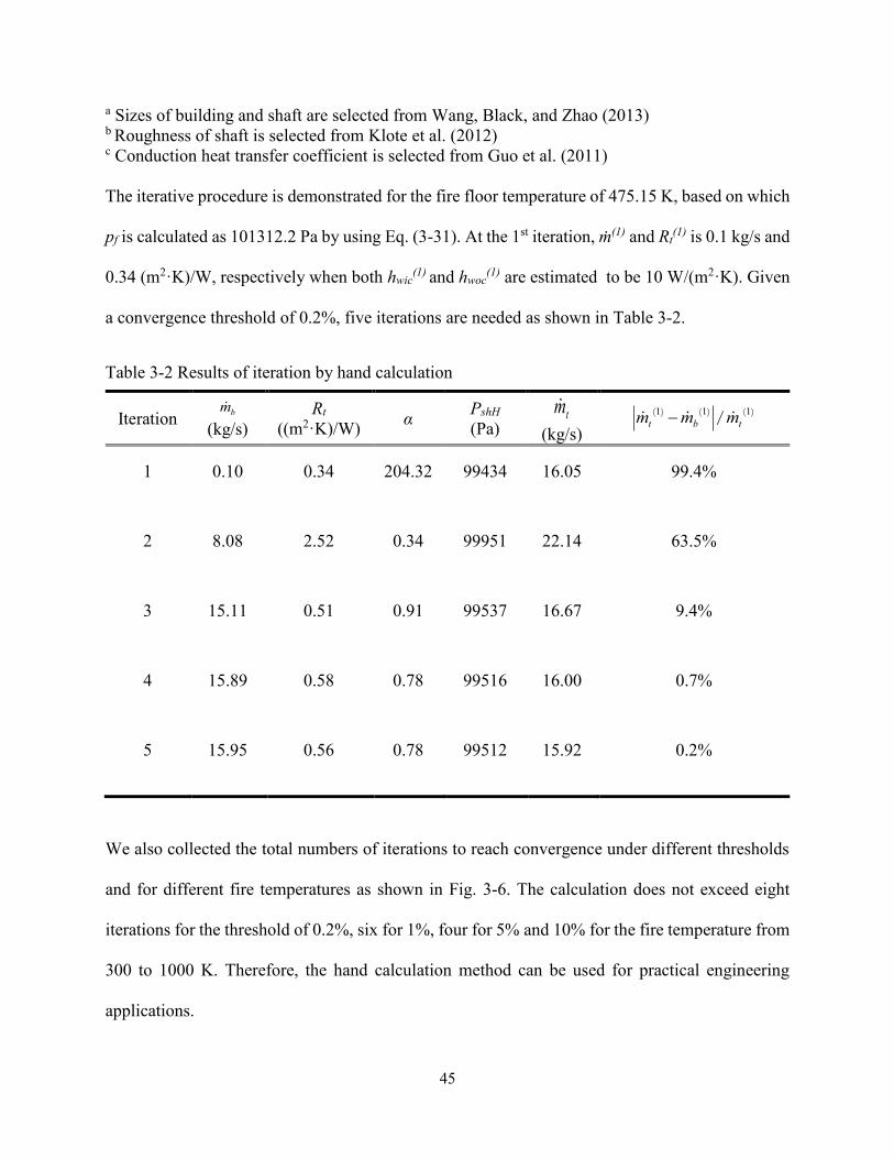
45

a Sizes of building and shaft are selected from Wang, Black, and Zhao (2013) b Roughness of shaft is selected from Klote et al. (2012) c Conduction heat transfer coefficient is selected from Guo et al. (2011)

The iterative procedure is demonstrated for the fire floor temperature of 475.15 K, based on which

pf is calculated as 101312.2 Pa by using Eq. (3-31). At the 1st iteration, ṁ(1) and Rt(1) is 0.1 kg/s and

0.34 (m2·K)/W, respectively when both hwic(1) and hwoc

(1) are estimated to be 10 W/(m2·K). Given

a convergence threshold of 0.2%, five iterations are needed as shown in Table 3-2.

Table 3-2 Results of iteration by hand calculation

Iteration bm

(kg/s)

Rt

((m2·K)/W) α

PshH

(Pa) tm

(kg/s)

)()()(/

111

tbt mmm

1 0.10 0.34 204.32 99434 16.05 99.4%

2 8.08 2.52 0.34 99951 22.14 63.5%

3 15.11 0.51 0.91 99537 16.67 9.4%

4 15.89 0.58 0.78 99516 16.00 0.7%

5 15.95 0.56 0.78 99512 15.92 0.2%

We also collected the total numbers of iterations to reach convergence under different thresholds

and for different fire temperatures as shown in Fig. 3-6. The calculation does not exceed eight

iterations for the threshold of 0.2%, six for 1%, four for 5% and 10% for the fire temperature from

300 to 1000 K. Therefore, the hand calculation method can be used for practical engineering

applications.

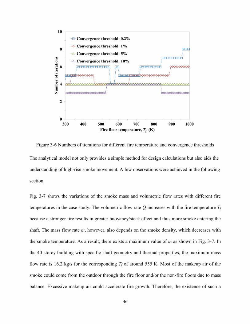
46

Figure 3-6 Numbers of iterations for different fire temperature and convergence thresholds

The analytical model not only provides a simple method for design calculations but also aids the

understanding of high-rise smoke movement. A few observations were achieved in the following

section.

Fig. 3-7 shows the variations of the smoke mass and volumetric flow rates with different fire

temperatures in the case study. The volumetric flow rate Q increases with the fire temperature Tf

because a stronger fire results in greater buoyancy/stack effect and thus more smoke entering the

shaft. The mass flow rate ṁ, however, also depends on the smoke density, which decreases with

the smoke temperature. As a result, there exists a maximum value of ṁ as shown in Fig. 3-7. In

the 40-storey building with specific shaft geometry and thermal properties, the maximum mass

flow rate is 16.2 kg/s for the corresponding Tf of around 555 K. Most of the makeup air of the

smoke could come from the outdoor through the fire floor and/or the non-fire floors due to mass

balance. Excessive makeup air could accelerate fire growth. Therefore, the existence of such a

47

maximum fire temperature and the corresponding maximum smoke mass flow rate could be an

important reference for the design of fire protection system, for the understanding of the effect of

high-rise shaft on the burning conditions at the fire floor, and consequently for the design of active

fire protection systems at the fire floor. The practical implications of the results are beyond the

scope this paper but can be covered in another study later.

The analytical model also provides important information on the risk assessment of the smoke

spread from the fire floor to higher floors mostly in terms of the location of the NPL. Fig. 3-8

shows the pressure profiles for the fire temperature of 375.15, 475.15 and 575.15 K. With the

increase of fire temperature, the overall shaft smoke temperature increases so the pressure

difference from the bottom to the top of the shaft becomes smaller. The location of NPL thus

increases with the fire temperature. In the current case, the NPL is 78 m for the fire of 375.15 K,

84 m for 475.15 K, and 90 m for 575.15 K. Smoke could enter non-fire floors above the NPL so a

higher NPL could result in a smaller section of non-fire floors subject to the smoke. However, with

the increase of the fire temperature, the elevated pressure difference above the NPL (Fig. 3-8)

could cause more smoke entry to these floors. Therefore, a detailed analysis should combine all

these effects based on the results from the current analytical model, which is beyond the scope of

this study but can be addressed in more details later.

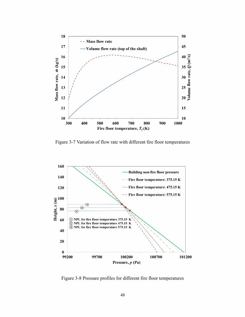
48

Figure 3-7 Variation of flow rate with different fire floor temperatures

Figure 3-8 Pressure profiles for different fire floor temperatures

49

3.4. Discussion

The case study only considers convective heat transfer but neglect radiation, which could be

significant during smoke spread. To apply the same method as convection, this study uses radiant

heat transfer coefficient to calculate radiation. Compared to convective heat transfer coefficient,

e.g. Eq. (3-34), radiant heat transfer coefficient depends on more factors, e.g. the geometry of the

shaft, gas compositions, gas and wall temperatures. Previous studies of analytical solutions often

neglected radiation (Sun et al. 2011; Ji et al. 2013), in which the effects of the neglecting were not

provided either. In this study, we discuss the effect of radiant heat transfer on the temperature

distributions with/without radiation through a sensitivity study of radiant heat transfer coefficients.

The same 40-storey building was used here for three different fire temperatures of 973.15 K (case

1), 773.15 K (case 2) and 573.15 K (case 3). The total heat transfer coefficients, hwi and hwo are the

sum of convective heat transfer coefficient and radiant heat transfer coefficient as Eqs. (3-37) and

(3-41) show. The convective heat transfer coefficients, hwic and hwoc are still calculated by Eq. (3-

34). For the radiation calculation, the smoke is assumed hot gas composed of water vapor and

carbon dioxide so the radiant heat transfer coefficient at the shaft interior wall could be calculated

by Eqs. (3-38) ~ (3-40) (Siegel and Howell 1993). The details about ai, ki, Le, CCO2, and εg can be

found in the literature(Siegel and Howell 1993). In real cases, a fire smoke can be loaded with

many other gases and/or soot, causing a higher radiation heat transfer. However, the method

presented here still applies if the radiant heat transfer coefficient can be provided. For the shaft

exterior wall, when the surface temperature is high, the radiation to the surrounding air inside the

building could become significant. The radiant heat transfer coefficient hwor could be calculated

by Eq. (3-42) (Hutcheon and Handegord 1983) with εw assumed one in this study.

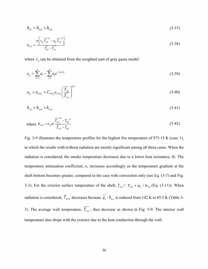
50

wirwicwi hhh (3-37)

wish

wigshg

wirTT

TaT

h

44

(3-38)

where g can be obtained from the weighted sum of gray gases model:

ei pLkn

i

i

n

i

ig eaa

11

(3-39)

5.0

222

wi

shCOCOCOg

T

TCaa (3-40)

worwocwo hhh (3-41)

where nfwo

nfwo

wworTT

TTh

44

(3-42)

Fig. 3-9 illustrates the temperature profiles for the highest fire temperature of 973.15 K (case 1),

in which the results with/without radiation are mostly significant among all three cases. When the

radiation is considered, the smoke temperature decreases due to a lower heat resistance, Rt. The

temperature attenuation coefficient, α, increases accordingly so the temperature gradient at the

shaft bottom becomes greater, compared to the case with convection only (see Eq. (3-7) and Fig.

3-3). For the exterior surface temperature of the shaft, woxT = woxnf hqT / (Eq. (3-11)). When

radiation is considered, woxT decreases because wox hq / is reduced from 142 K to 85.5 K (Table 3-

3). The average wall temperature, woT , thus decrease as shown in Fig. 3-9. The interior wall

temperature also drops with the exterior due to the heat conduction through the wall.

51

Figure 3-9 Comparison of temperature profiles with/without radiation for the fire temperature of

973.15 K (case1)

Table 3-3 Comparison of the results with/without radiation in case 1

hwo (W/(m2∙K)) m (kg/s) Tf -TshH (K) xq (W/m2) wox hq / (K)

Without radiation 6.8 15.2 443 966 142

With radiation 14.3 15 547 1180 85.5

To quantify the difference of the predicted temperatures with radiation, Tc&r, and without radiation,

Tc, this study use normalized mean square error (NMSE) (ASTM D5157-97 2008).

n

i

ircic

rcc

TTnTT

NMSE1

2

,&,

&

11 (3-43)

The calculated temperatures at every eight meters in the shaft were used to calculate the NMSE.

Table 3-4 lists the NMSEs for Tsh, Twi and Two. It shows that the largest difference is 1.8% for the

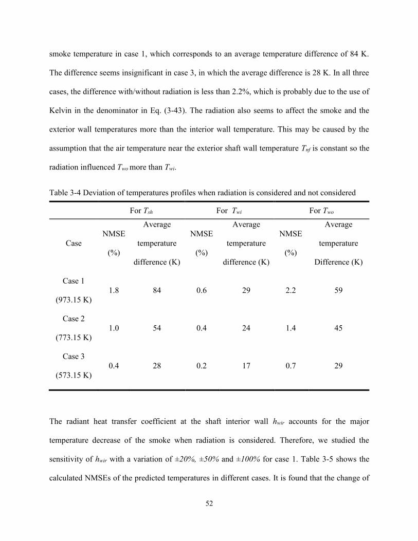
52

smoke temperature in case 1, which corresponds to an average temperature difference of 84 K.

The difference seems insignificant in case 3, in which the average difference is 28 K. In all three

cases, the difference with/without radiation is less than 2.2%, which is probably due to the use of

Kelvin in the denominator in Eq. (3-43). The radiation also seems to affect the smoke and the

exterior wall temperatures more than the interior wall temperature. This may be caused by the

assumption that the air temperature near the exterior shaft wall temperature Tnf is constant so the

radiation influenced Two more than Twi.

Table 3-4 Deviation of temperatures profiles when radiation is considered and not considered

For Tsh For Twi For Two

Case NMSE

(%)

Average

temperature

difference (K)

NMSE

(%)

Average

temperature

difference (K)

NMSE

(%)

Average

temperature

Difference (K)

Case 1

(973.15 K)

1.8 84 0.6 29 2.2 59

Case 2

(773.15 K)

1.0 54 0.4 24 1.4 45

Case 3

(573.15 K)

0.4 28 0.2 17 0.7 29

The radiant heat transfer coefficient at the shaft interior wall hwir accounts for the major

temperature decrease of the smoke when radiation is considered. Therefore, we studied the

sensitivity of hwir with a variation of ±20%, ±50% and ±100% for case 1. Table 3-5 shows the

calculated NMSEs of the predicted temperatures in different cases. It is found that the change of

53

hwir affects the smoke and the interior wall temperatures more than the exterior as expected. In this

case, the over-estimations of hwir generally cause fewer changes than the under-estimations when

the radiation was considered. The largest variation (0.57%) occurs when hwir is 100% under-

estimated in this case, corresponding to an average temperature deviation of only 46 K. Therefore,

the temperature predictions seem not quite sensitive to the change of radiant heat transfer

coefficient in this case.

Table 3-5 NMSEs of predicted temperatures for different radiant heat transfer coefficients

Case

Temperature

profile

Variations of radiant heat transfer coefficient hwir (%)

-100% -50% -20% 20% 50% 100%

Case 1

(973.15 K)

For Tsh 0.57 0.09 0.01 0.01 0.04 0.12

For Twi 0.54 0.08 0.01 0.01 0.04 0.11

For Two 0.10 0.02 0.00 0.00 0.01 0.02

Note that among other cases when radiation is considered, heat transfer coefficients may vary

significantly along the shaft height, because radiation is the fourth order of absolute temperatures.

In this case, the assumption that heat transfer coefficients do not vary along the height may not be

applicable. However, the limitation could be overcome by dividing the shaft into several vertical

sub-sections, for each of which the foregoing analytical model can be applied with different heat

transfer coefficients.

3.5. Conclusion

This study developed an analytical model for the smoke spread through a vertical shaft in a high-

rise building during fires when the shaft is with a given constant smoke flow rate and with the

54

smoke purely driven by stack effect. The associated equations include heat and mass balance, and

mechanical energy equations, which form a coupled smoke heat and mass transfer problem

through the shaft. This study presented the hand calculation method to solve the coupled problem

and demonstrated it in a case study of the smoke spread in a 40-storey building. The effects of the

radiant heat transfer on the calculated temperature profiles were also discussed. The study reached

the following major conclusions:

(1). The temperature attenuation coefficient, α, is an important parameter for the solutions of the

coupled problem, because the temperature profiles of smoke and shaft wall are both shown to be

exponential functions of α.

(2). The analytical solution provides the important information for the risk assessment of the smoke

spread from the fire floor to higher floors, including shaft top temperature, maximum mass flow

rate and corresponding fire floor temperature, and location of NPL.

(3). In the case study of the 40-storey building, only a few hand calculation iterations were needed

to obtain the analytical solution so the analytical model is very practical for real design problems.

(4). The effect of radiation on temperature calculations increases with fire temperatures. The

sensitivity study of the radiant heat transfer coefficient shows that the overestimation of the

radiation generally affects the temperature calculations less than the underestimation. Generally,

the temperature calculations seem not quite sensitive to the change of the radiant heat transfer

coefficients at the shaft interior wall in the case studied.

Some limitations about the current analytical solution were also noted. The current solution does

not consider the situation when heat transfer coefficients vary significantly along the shaft height.

The limitation could be overcome by dividing the shaft into several vertical sub-sections, for each

55

of which the analytical model can be applied with variable heat transfer coefficients with the height

of the shaft.

56

Chapter 4 Dimensionless Analytical Solutions for Steady-state Heat and

Mass Transfer through High-rise Shafts

Abstract

Analytical solutions in terms of dimensionless numbers for the smoke spread through high-rise

shafts during fires are essential to provide a fundamental understanding of smoke transport physics,

which is a complex coupled heat and mass transfer problem. Existing solutions are often

dimensional based on simplification of the problem such as assuming adiabatic conditions. In order

to obtain the dimensionless analytical solutions, energy balance equation, mechanical energy

equation and mass balance equation were established for high-rise smoke spread under both

mechanical and natural venting conditions. Experiments were deigned and conducted on two

different size and material shafts, and the measured results were compared to the dimensionless

analytical solutions. It was found that the dimensionless analytical solutions could predict

temperature profiles, mass flow rate and neutral plane level accurately. The effect of the adiabatic

assumption on the accuracy was also discussed. For example, due to the adiabatic assumption, the

error of the calculated mass flow rate required during mechanical venting to maintain a high-rise

shaft smoke free was found to increase with a dimensionless number, ω, defined by the geometrical

and thermal properties of the shaft.

4.1. Introduction

Fires in high-rise buildings are often disastrous, causing many injuries, fatalities and huge

economic losses. Such notorious fires as the Winecoff Hotel fire at Atlanta, US (December 7, 1946)

caused 119 deaths, and the MGM Grand Hotel fire at Las Vegas, NV (November 21, 1980) led to

the deaths of 85 people and 600 injured (Tamura 1994). A most recent high-rise fire, the 63-story

57

Address Downtown Dubai Hotel fire, occurred on New Year’s Eve of 2016, and continued to

generate smoke on the next day even after the fire was put down (“Dubai Hotel Fire Could Have

Been Worse” 2016; Chappell 2016). Although luckily no deaths seem reported, the estimated

repairs and business interruption exceeds $100 million dollars. Smoke generated from fires often

spreads quickly throughout a building, often even faster than the fire itself, especially in a high-

rise building, carrying toxic gases responsible for the majority of fatalities (Gann et al. 1994) with

elevated temperatures causing spread damages of upholsteries and structures.

In typical high-rise buildings, about 95% or more of the upward movement of smoke attributes to

the spreads through shafts (Tamura 1994), e.g. stairs, elevators, light wells, ventilation ducts. High-

rise smoke control using pressurization systems becomes a popular option since the 1960s: by

injecting clean air with mechanical fans into a shaft enclosure such that the pressure in the shaft is

greater than the adjacent fire compartment, the pressurization systems are intended to prevent

smoke leaking from its sources (Lay 2014). However, the pressurization systems have been found

not to always work as expected, especially for high-rise shafts with strong stack effect, also known

as chimney effect where shafts act like chimneys and smoke tends to spreads upwards due to

buoyancy, and floor-to-floor variations in flow resistance (Klote 2011). It was estimated that 35%

of pressurization systems might fail to function as intended (Lay 2014). A pressurization system

often acts against the stack effect so its performance heavily relies on the strength of the stack

effect, which could be subject to many variants, e.g. fire strengths and ambient weather conditions.

An alternative approach is the use of shafts as smoke venting routes through which the smoke

would be properly channeled to spread upwards, and eventually be exhausted at the top of the

shafts to the outside of a building. Instead of fighting against the stack effect, this method of shaft

58

smoke ventilation takes advantage of naturally-generated stack effect due to buoyancy, aided by

mechanical fan systems when necessary, and thus gains much attentions lately.

These shaft smoke ventilation systems allow fire smoke to spread through expectedly well-

engineered routes of shafts so it is critical to understand the dynamic and thermal properties of the

smoke along its route to the exit points, specifically smoke flow rates, smoke temperature and

pressure distributions. Previous studies have been conducted using various experimental,

mathematical and numerical techniques. Ji and Shi performed extensive experiments to investigate

the transport characteristics of thermal plume in a ventilated stairwell with two or multiple

openings (Jie Ji et al. 2015; Li et al. 2014; Ji et al. 2013; Shi et al. 2014a). Harmthy proposed a

Fire Drainage System to remove the heat and induced convection smoke flow from a fire through

a series of shafts to reduce the spread of fire from the region of fire source (Lay 2014; Harmathy

and Oleszkiewicz 1987). Design principles of this system were also introduced based on the

assumption of constant gas temperature (Harmathy and Oleszkiewicz 1987) but the heat transfer

between the smoke and the shaft walls was not considered, i.e. under adiabatic conditions. Similar

to the Fire Drainage System, the Beetham Tower system was developed to use an air inlet shaft to

exhaust smoke from the fire floor aided by a mechanical fan system (Lay 2014). Klote studied the

smoke ventilation control of stairwells in tall buildings by a tenability analysis based on

computational fluid dynamics (CFD) and multizone network modeling. It was concluded that the

stairwell smoke ventilation is a feasible approach (Klote 2011). Qi et al. (Qi, Wang, and

Zmeureanu 2014a) developed an analytical model of smoke movement in high-rise shafts.

Different from other analytical models, heat transfer between smoke and the shaft boundaries was

considered. Based on the analytical model, a hand calculation method and empirical equations

59

were developed for the calculation of temperature distribution, mass flow rate and pressure inside

the shaft (Qi, Wang, and Zmeureanu 2014b; Qi, Wang, and Zmeureanu 2016).

However, most of the previous studies were conducted on specific buildings and shafts. As a result

the generalization of the conclusions to other cases may need further verifications. Therefore, there

exists a gap of research that the solutions to smoke flow rates, temperature and pressure

distributions, preferably expressed in dimensionless analytical forms, should be developed for a

better understanding of the thermal aerodynamics of shaft smoke ventilations. The dimensionless

solutions could also benefit the research on the similitude and scale modeling analysis of a high-

rise building, for which the sheer size of the structure often makes full-size tests impractical.

This paper reported the development of dimensionless analytical solutions of smoke spread in non-

adiabatic high-rise shafts during fires. Conservation equations of thermal energy, mechanical

energy, and mass were developed in dimensionless forms for both mechanical and natural smoke

ventilations. A series of experiments were then conducted on two scaled shafts with different

dimensions and materials, and used to validate the developed dimensionless analytical solutions

by comparing temperature distribution, mass flow rate, pressure distributions, and neutral plane

levels (NPL). As an example of demonstration, we applied the dimensionless analytical solution

developed in this study to calculating the minimum mechanical venting rate required to maintain

a full-size high-rise shaft free of smoke, and compared to the result if the conventional adiabatic

assumption is used. The comparison helps to show the impact of the adiabatic assumption on the

accuracy of the calculation.

60

4.2. Theory

Smoke spread inside high-rise shafts may be generalized by the schematic in Fig. 4-1. When

mechanical smoke ventilation is used, a fan is installed at the top of the shaft. In comparison, the

fan is replaced by an opening at the top for natural venting/ventilation of the smoke. The objective

of this section is to develop dimensionless analytical solutions for these two venting systems, for

which the following assumptions are used:

A fire is located at the first floor of the building with a fire strength defined by the fire

temperature.

Smoke movement in the shaft is one-dimensional at steady state.

The outdoor air temperature and the building temperature at non-fire floors are constant.

Specific heat capacity of the smoke, Cp, is constant.

The smoke is assumed to be incompressible and viscous but thermally expansible satisfying

the ideal gas law.

No smoke leaks through shaft walls.

Heat transfer coefficients (either due to convection or radiation) are constant and do not vary

along the height of the shaft.

The temperature of the fire floor is uniform and maintained at the fire smoke temperature (Qi,

Wang, and Zmeureanu 2014a).

The smoke flow inside the shaft could be assumed as one-dimensional steady-state flow (Qi,

Wang, and Zmeureanu 2014a; Li et al. 2014).

The friction loss of the flow due to interior shaft wall is neglected (Qi, Wang, and Zmeureanu

2016).

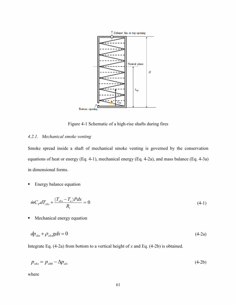
61

Figure 4-1 Schematic of a high-rise shafts during fires

4.2.1. Mechanical smoke venting

Smoke spread inside a shaft of mechanical smoke venting is governed by the conservation

equations of heat or energy (Eq. 4-1), mechanical energy (Eq. 4-2a), and mass balance (Eq. 4-3a)

in dimensional forms.

Energy balance equation

0

t

ashxshxP

R

PdxTTdTCm

)( (4-1)

Mechanical energy equation

0 gdxdp shxshx (4-2a)

Integrate Eq. (4-2a) from bottom to a vertical height of x and Eq. (4-2b) is obtained.

elxshshx ppp 0 (4-2b)

where

62

1

10

0

Hx

a

ax

shxelx

e

RT

Hgpgdxp

/

ln (4-2c)

Mass balance equation

mmm bt (4-3a)

where ṁb can be calculated by the orifice equation:

)/()()( aashabdshaabdb RTpppACppACm 00000 22 (4-3b)

For mechanical venting, mass flow rate is controlled by mechanical fan, so psh0 is calculated by

Eq. (4-3b)

To convert the conservation equations into dimensionless forms, a series of dimensionless numbers

are defined as follows.

Dimensionless temperature, θsh

ash

ashxsh

TT

TT

0

(4-4)

Dimensionless fire temperature,

a

ash

T

TT 0

(4-5)

Temperature attenuation coefficient, α

tPRCm

PH

(4-6)

where wowi

th

W

hR

11

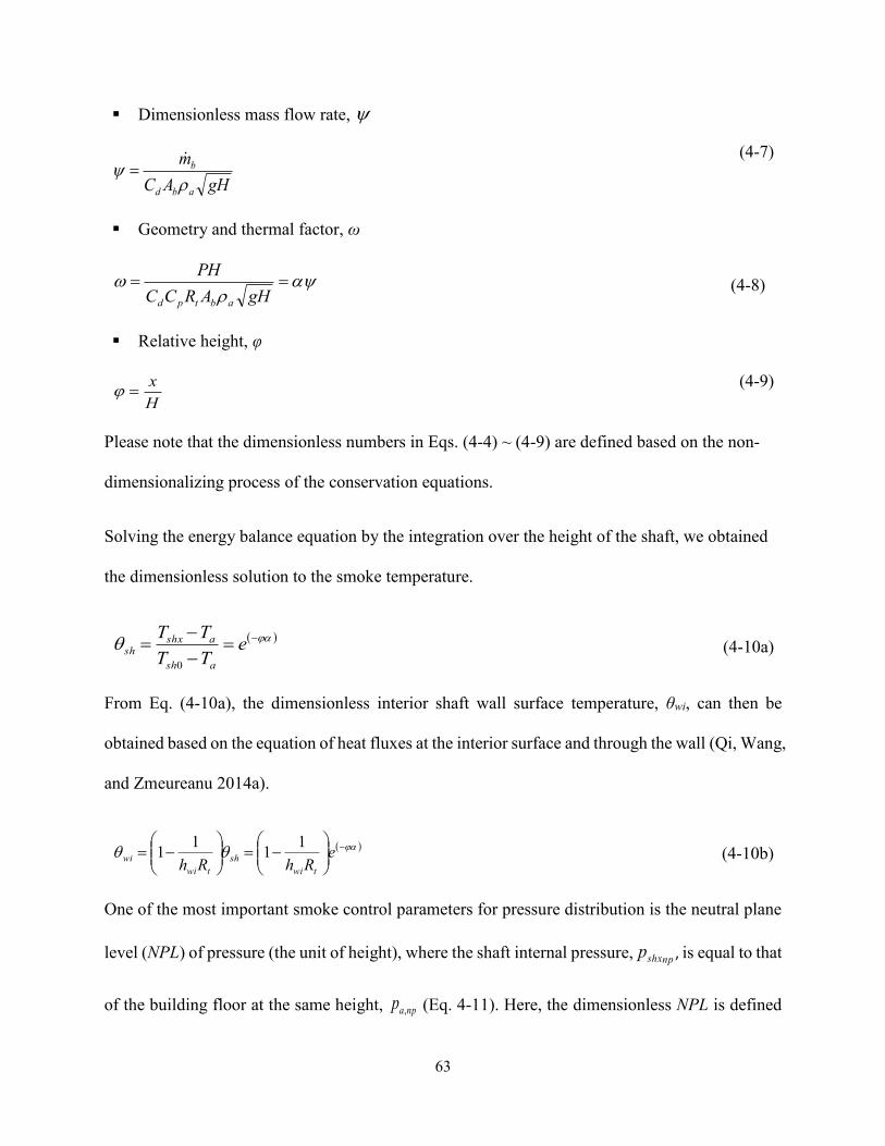
63

Dimensionless mass flow rate,

gHAC

m

abd

b

(4-7)

Geometry and thermal factor, ω

gHARCC

PH

abtpd

(4-8)

Relative height, φ

H

x

(4-9)

Please note that the dimensionless numbers in Eqs. (4-4) ~ (4-9) are defined based on the non-

dimensionalizing process of the conservation equations.

Solving the energy balance equation by the integration over the height of the shaft, we obtained

the dimensionless solution to the smoke temperature.

e

TT

TT

ash

ashxsh

0

(4-10a)

From Eq. (4-10a), the dimensionless interior shaft wall surface temperature, θwi, can then be

obtained based on the equation of heat fluxes at the interior surface and through the wall (Qi, Wang,

and Zmeureanu 2014a).

e

RhRh twi

sh

twi

wi

11

11 (4-10b)

One of the most important smoke control parameters for pressure distribution is the neutral plane

level (NPL) of pressure (the unit of height), where the shaft internal pressure,npshxp , is equal to that

of the building floor at the same height, npap , (Eq. 4-11). Here, the dimensionless NPL is defined

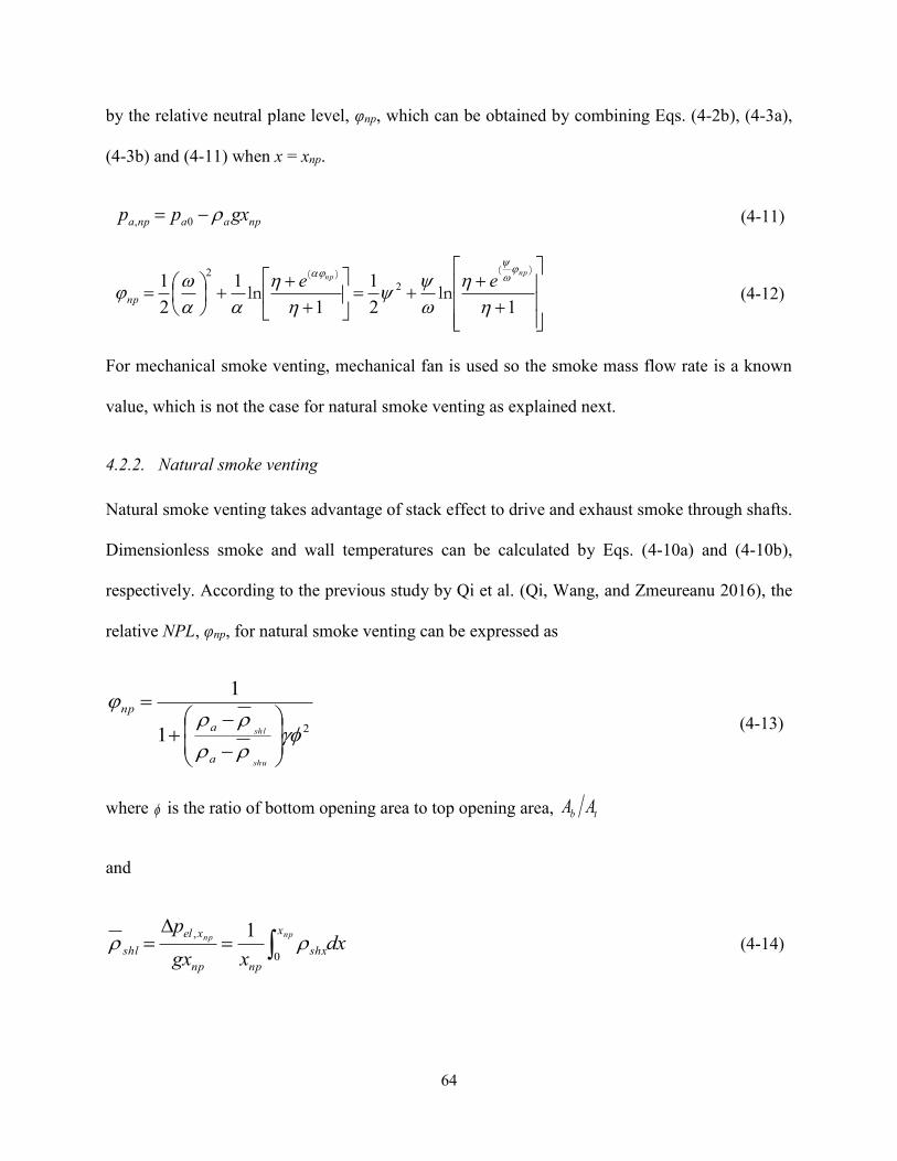
64

by the relative neutral plane level, φnp, which can be obtained by combining Eqs. (4-2b), (4-3a),

(4-3b) and (4-11) when x = xnp.

npaanpa gxpp 0, (4-11)

12

1

1

1

2

1 2

2

)()(

lnln

npnp ee

np (4-12)

For mechanical smoke venting, mechanical fan is used so the smoke mass flow rate is a known

value, which is not the case for natural smoke venting as explained next.

4.2.2. Natural smoke venting

Natural smoke venting takes advantage of stack effect to drive and exhaust smoke through shafts.

Dimensionless smoke and wall temperatures can be calculated by Eqs. (4-10a) and (4-10b),

respectively. According to the previous study by Qi et al. (Qi, Wang, and Zmeureanu 2016), the

relative NPL, φnp, for natural smoke venting can be expressed as

21

1

shu

shl

a

a

np (4-13)

where is the ratio of bottom opening area to top opening area, tb AA

and

npnp

x

shx

npnp

xel

shl dxxgx

p

0

1

,

(4-14)

65

H

xshx

npnp

shudx

xH

1 (4-15)

Take Eqs. (4-14) and (4-15) into Eq. (4-13), the dimensionless solution of NPL could be

obtained:

2

1

11

1

11

1

1

)(

)(

)(

ln

ln

np

np

e

e

e

np

np

np (4-16)

To obtain the mass flow rate, we apply the orifice equation to the top opening of the shaft as Eq.

(4-17) shows.

shHaaHshHtdaHshHshHtdt RTpppACppACm /)(2)(2 0 (4-17)

By combining Eqs. (4-2b), (4-3a), (4-3b), (4-8) and (4-17) when x = H, the dimensionless mass

flow rate, , for natural venting can be derived.

2

2

2

1

1

112

eln

(4-18)

Where is the dimensionless smoke temperature at the top of the shaft, )( eTT ashH 1 .

Table 1 summarizes the dimensionless solutions for both mechanical and natural venting. A few

observations can be made here:

The temperature profile, θsh, is the function of α, in which α is only associated with the

geometrical and thermal properties of the smoke and the shaft

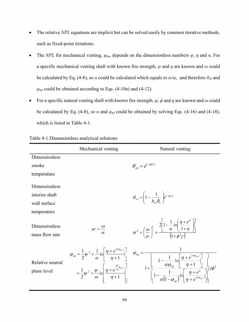
66

The relative NPL equations are implicit but can be solved easily by common iterative methods,

such as fixed-point iterations.

The NPL for mechanical venting, φnp, depends on the dimensionless numbers ψ, η and α. For

a specific mechanical venting shaft with known fire strength, ψ and η are known and ω could

be calculated by Eq. (4-8), so α could be calculated which equals to ω/ψ, and therefore θsh and

φnp could be obtained according to Eqs. (4-10a) and (4-12).

For a specific natural venting shaft with known fire strength, ψ, ϕ and η are known and ω could

be calculated by Eq. (4-8), so α and φnp could be obtained by solving Eqs. (4-16) and (4-18),

which is listed in Table 4-1.

Table 4-1 Dimensionless analytical solutions

Mechanical venting Natural venting

Dimensionless

smoke

temperature

esh

Dimensionless

interior shaft

wall surface

temperature

e

Rh twi

wi

11

Dimensionless

mass flow rate

2

2

2

1

1

112

eln

Relative neutral

plane level

12

1

1

1

2

1

2

2

)(

)(

ln

ln

np

np

e

enp

2

1

11

1

11

1

1

)(

)(

ln

ln

np

np

e

e

e

np

np

np

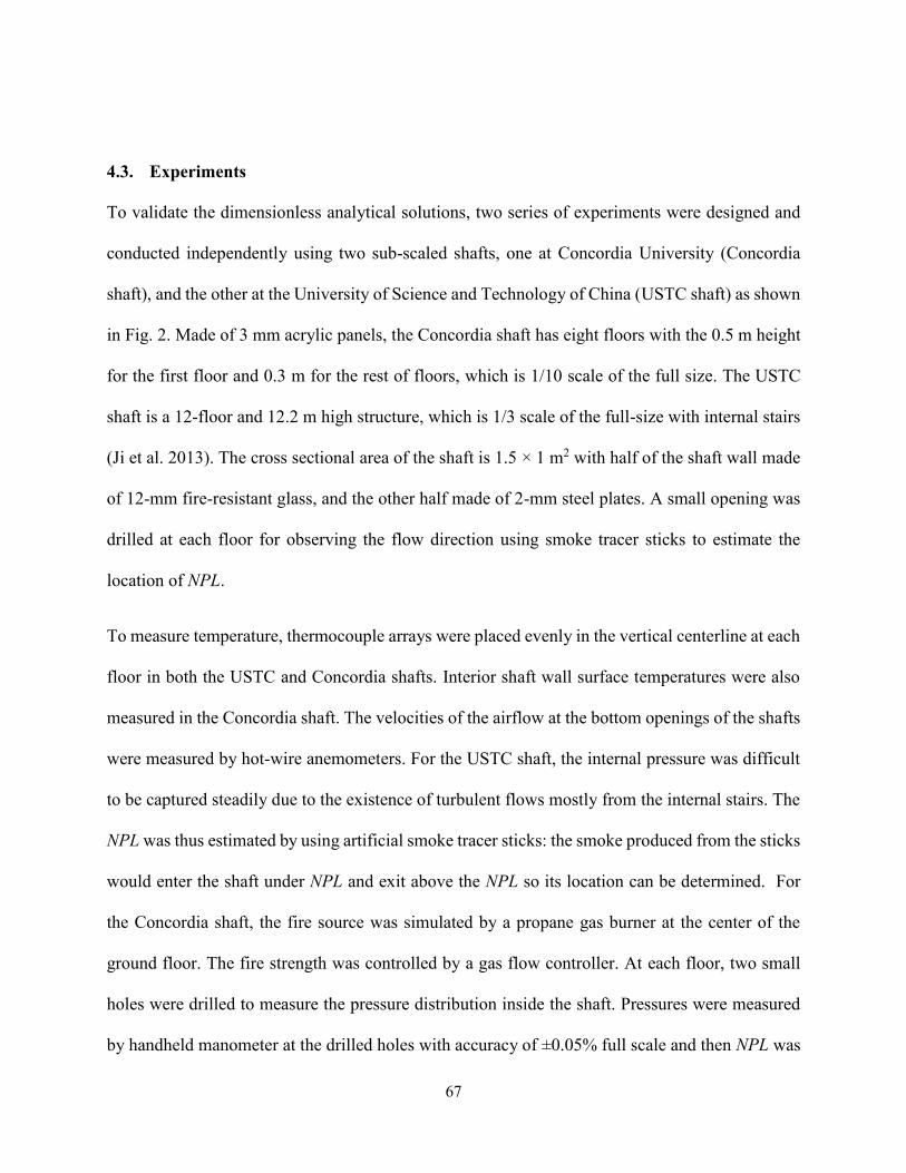
67

4.3. Experiments

To validate the dimensionless analytical solutions, two series of experiments were designed and

conducted independently using two sub-scaled shafts, one at Concordia University (Concordia

shaft), and the other at the University of Science and Technology of China (USTC shaft) as shown

in Fig. 2. Made of 3 mm acrylic panels, the Concordia shaft has eight floors with the 0.5 m height

for the first floor and 0.3 m for the rest of floors, which is 1/10 scale of the full size. The USTC

shaft is a 12-floor and 12.2 m high structure, which is 1/3 scale of the full-size with internal stairs

(Ji et al. 2013). The cross sectional area of the shaft is 1.5 × 1 m2 with half of the shaft wall made

of 12-mm fire-resistant glass, and the other half made of 2-mm steel plates. A small opening was

drilled at each floor for observing the flow direction using smoke tracer sticks to estimate the

location of NPL.

To measure temperature, thermocouple arrays were placed evenly in the vertical centerline at each

floor in both the USTC and Concordia shafts. Interior shaft wall surface temperatures were also

measured in the Concordia shaft. The velocities of the airflow at the bottom openings of the shafts

were measured by hot-wire anemometers. For the USTC shaft, the internal pressure was difficult

to be captured steadily due to the existence of turbulent flows mostly from the internal stairs. The

NPL was thus estimated by using artificial smoke tracer sticks: the smoke produced from the sticks

would enter the shaft under NPL and exit above the NPL so its location can be determined. For

the Concordia shaft, the fire source was simulated by a propane gas burner at the center of the

ground floor. The fire strength was controlled by a gas flow controller. At each floor, two small

holes were drilled to measure the pressure distribution inside the shaft. Pressures were measured

by handheld manometer at the drilled holes with accuracy of ±0.05% full scale and then NPL was

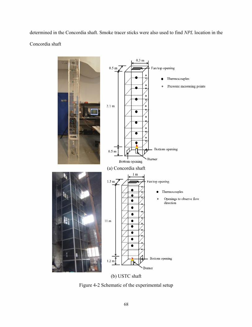
68

determined in the Concordia shaft. Smoke tracer sticks were also used to find NPL location in the

Concordia shaft

(a) Concordia shaft

(b) USTC shaft

Figure 4-2 Schematic of the experimental setup

69

Table 4-2 Experiments design

Geometry and thermal factor, ω Dimensionless

fire temperature, η

Dimensionless mass

flow rates, ψ

Mechanical venting

Concordia shaft1

0.15 0.29 0.33~0.61

0.15 0.35 0.4~0.63

USTC shaft2

0.3 0.12 0.17~0.35

0.3 0.16 0.27~0.39

Natural venting

Concordia shaft3

0.08 0.10 /

0.11 0.18 /

0.12 0.28 /

1Cd=0.65(Dols and Polidoro 2015), Rt = 0.5 (m2·K)/W 2Cd=0.23(Ji et al. 2013), Rt = 0.27 (m2·K)/W 3Cd=0.65(Dols and Polidoro 2015), Rt = 0.5~0.7 (m2·K)/W

Fire strength in terms of dimensionless fire temperature, η, and dimensionless mass flow rates, ψ,

were reported in Table 4-2. Nine experiments were conducted for the Concordia shaft and 24

experiments were conducted on the USTC shaft for mechanical venting. For natural venting, three

experiments were performed on the Concordia shaft. Note that the USTC tests were conducted

independently before the dimensionless analytical solutions in this study were developed mostly

at Concordia, so many dimensionless numbers were with different values, and they were not

intentionally made to be the same.

4.4. Results and discussion

4.4.1. Mechanical smoke venting

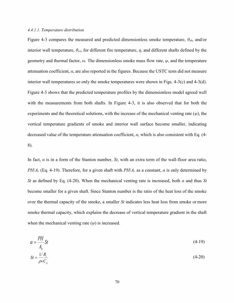
70

4.4.1.1. Temperature distribution

Figure 4-3 compares the measured and predicted dimensionless smoke temperature, θsh, and/or

interior wall temperature, θwi, for different fire temperature, η, and different shafts defined by the

geometry and thermal factor, ω. The dimensionless smoke mass flow rate, ψ, and the temperature

attenuation coefficient, α, are also reported in the figures. Because the USTC tests did not measure

interior wall temperatures so only the smoke temperatures were shown in Figs. 4-3(c) and 4-3(d).

Figure 4-3 shows that the predicted temperature profiles by the dimensionless model agreed well

with the measurements from both shafts. In Figure 4-3, it is also observed that for both the

experiments and the theoretical solutions, with the increase of the mechanical venting rate (ψ), the

vertical temperature gradients of smoke and interior wall surface become smaller, indicating

decreased value of the temperature attenuation coefficient, α, which is also consistent with Eq. (4-

8).

In fact, α is in a form of the Stanton number, St, with an extra term of the wall-floor area ratio,

PH/Ac (Eq. 4-19). Therefore, for a given shaft with PH/Ac as a constant, α is only determined by

St as defined by Eq. (4-20). When the mechanical venting rate is increased, both α and thus St

become smaller for a given shaft. Since Stanton number is the ratio of the heat loss of the smoke

over the thermal capacity of the smoke, a smaller St indicates less heat loss from smoke or more

smoke thermal capacity, which explains the decrease of vertical temperature gradient in the shaft

when the mechanical venting rate (ψ) is increased.

StA

PH

h

(4-19)

p

t

vC

RSt

/1 (4-20)

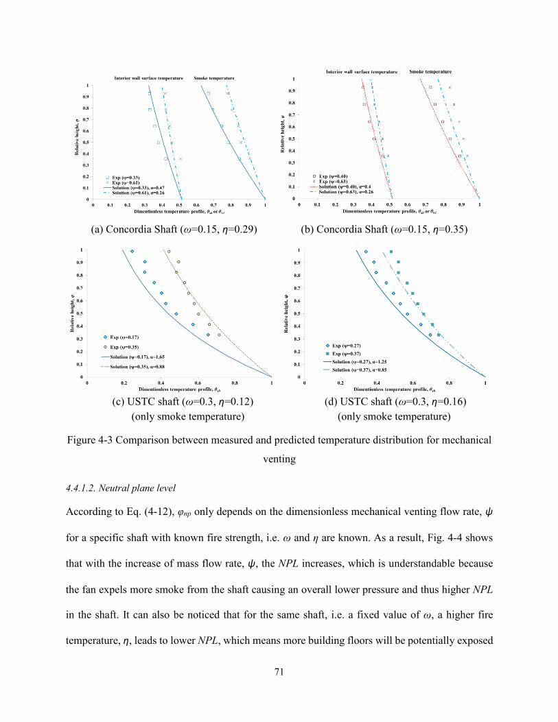
71

(a) Concordia Shaft (ω=0.15, η=0.29) (b) Concordia Shaft (ω=0.15, η=0.35)

(c) USTC shaft (ω=0.3, η=0.12) (d) USTC shaft (ω=0.3, η=0.16)

(only smoke temperature) (only smoke temperature)

Figure 4-3 Comparison between measured and predicted temperature distribution for mechanical

venting

4.4.1.2. Neutral plane level

According to Eq. (4-12), φnp only depends on the dimensionless mechanical venting flow rate, ψ

for a specific shaft with known fire strength, i.e. ω and η are known. As a result, Fig. 4-4 shows

that with the increase of mass flow rate, ψ, the NPL increases, which is understandable because

the fan expels more smoke from the shaft causing an overall lower pressure and thus higher NPL

in the shaft. It can also be noticed that for the same shaft, i.e. a fixed value of ω, a higher fire

temperature, η, leads to lower NPL, which means more building floors will be potentially exposed

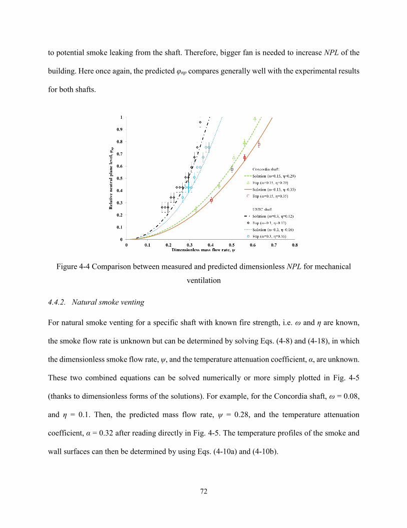
72

to potential smoke leaking from the shaft. Therefore, bigger fan is needed to increase NPL of the

building. Here once again, the predicted φnp compares generally well with the experimental results

for both shafts.

Figure 4-4 Comparison between measured and predicted dimensionless NPL for mechanical

ventilation

4.4.2. Natural smoke venting

For natural smoke venting for a specific shaft with known fire strength, i.e. ω and η are known,

the smoke flow rate is unknown but can be determined by solving Eqs. (4-8) and (4-18), in which

the dimensionless smoke flow rate, ψ, and the temperature attenuation coefficient, α, are unknown.

These two combined equations can be solved numerically or more simply plotted in Fig. 4-5

(thanks to dimensionless forms of the solutions). For example, for the Concordia shaft, ω = 0.08,

and η = 0.1. Then, the predicted mass flow rate, ψ = 0.28, and the temperature attenuation

coefficient, α = 0.32 after reading directly in Fig. 4-5. The temperature profiles of the smoke and

wall surfaces can then be determined by using Eqs. (4-10a) and (4-10b).

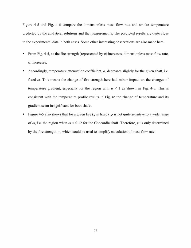
73

Figure 4-5 and Fig. 4-6 compare the dimensionless mass flow rate and smoke temperature

predicted by the analytical solutions and the measurements. The predicted results are quite close

to the experimental data in both cases. Some other interesting observations are also made here:

From Fig. 4-5, as the fire strength (represented by η) increases, dimensionless mass flow rate,

ψ, increases.

Accordingly, temperature attenuation coefficient, α, decreases slightly for the given shaft, i.e.

fixed ω. This means the change of fire strength here had minor impact on the changes of

temperature gradient, especially for the region with α < 1 as shown in Fig. 4-5. This is

consistent with the temperature profile results in Fig. 6: the change of temperature and its

gradient seem insignificant for both shafts.

Figure 4-5 also shows that for a given fire (η is fixed), ψ is not quite sensitive to a wide range

of ω, i.e. the region when ω < 0.12 for the Concordia shaft. Therefore, ψ is only determined

by the fire strength, η, which could be used to simplify calculation of mass flow rate.

74

Figure 4-5 The predicted and measured dimensionless smoke flow rates, ψ, under different

temperature attenuation coefficients, α, for different shaft properties (ω), and fire temperatures

(η) during the natural venting of Concordia shaft.

75

Figure 4-6 Temperature distributions predicted by dimensionless analytical solutions and

measured by experiments for natural venting of Concordia shaft.

Due to the minor change of α with the increase of fire strength as it indicated by Fig. 4-6, the fire

strength has little influence on the relative NPL for natural venting. This is consistent with the

previous study by Li et al. (2014). Table 4-3 compares φnp of measured and predicted relative NPL

for natural venting. When the fire strength, η, increases from 0.1 to 0.28, the measured φnp is around

0.46±0.05 is close to the predicted one by dimensionless model, which is around 0.44.

Table 4-3 Measured and predicted relative NPL by dimensionless analytical model for natural

venting of Concordia shaft.

Measured results Predicted by dimensionless model

Relative NPL 0.46 ± 0.05 0.44

76

4.5. Discussion

For simplicity, many previous studies often assumed a shaft to be adiabatic (Zhang et al. 2008;

Klote et al. 2012), for which the literature found that the error of the predicted NPL location could

be significant (Yang et al. 2012). An inaccurate prediction of NPL could cause a poorly designed

or even failed mechanical venting system, because the mechanical fan is expected to achieve a

NPL as high as possible, preferably to the top of the shaft so there would be zero chance that non-

fire building floors could be potentially exposed to toxic smoke from the shaft.

In this section, with the help of the dimensionless analytical solutions developed here, we are able

to discuss about the errors from the adiabatic assumption. The required mechanical venting rate to

keep a shaft smoke free can be found by letting φnp = 1 in Eq. (4-12) to obtain Eq. (4-21), from

which the dimensionless fan flow rate required to achieve the highest NPL (the top of the shaft)

can be calculated based on geometrical and thermal parameters of the shaft, i.e. ω, and fire strength,

i.e. η. For comparison, the required fan flow under the adiabatic assumption can also be derived:

for Eq. (4-21) under the adiabatic assumption, setting the geometry and thermal factor of a shaft,

ω = 0, and finding its limit, we can obtain Eq. (4-22) if the adiabatic assumption is applied. It

shows that Eq. (4-22) is only a function of fire strength, η, regardless of the shaft geometrical and

thermal properties. The relative error of the adiabatic assumption can then be defined by Eq. (4-

23) when compared to the non-adiabatic situation.

12

11 2

adnoneadnonadnon ln

(4-21)

1

2

ad

(4-22)

77

adnon

adnonad

adnon

adnonad

m

mm

=error Relative

(4-23)

where “ad” is for “adiabatic” and “non-ad” for “non-adiabatic”.

Equation 4-23 is plotted for a wide range of building parameters (ω) and fire (η) as shown in Fig.

4-7. Here are a few interesting observations:

With the increase of ω, the error due to adiabatic assumption increases. It can be explained by

that: a greater P, H or smaller values of Rt increase ω, and thus more heat loss from smoke to

shaft wall. So neglecting heat transfer leads to more error under the adiabatic assumption.

With the decrease of η, the error also increases. Therefore, for a shaft with bigger ω and/or

smaller η, the adiabatic assumption leads to more errors.

Here, to put the analysis in the context of real buildings, consider a 40-storey high-rise stairwell

with the detailed specification shown in Table 4. If all the infiltration area is lumped as a part of

the bottom opening area, which is often done to consider leakages on shaft walls, ω is around 1.5.

The relative error of the adiabatic assumption is about 18% for a fire with η = 2, corresponding to

a high-rise fire of 5 MW. The error of 18% means an overestimation of 18% of the mechanical

venting fan capacity in terms of mass flow rate to keep the high-rise shaft smoke free.

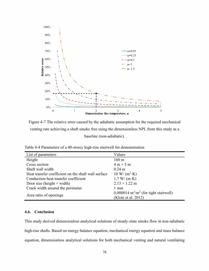
78

Figure 4-7 The relative error caused by the adiabatic assumption for the required mechanical

venting rate achieving a shaft smoke free using the dimensionless NPL from this study as a

baseline (non-adiabatic).

Table 4-4 Parameters of a 40-storey high-rise stairwell for demonstration

List of parameters Values

Height 160 m

Cross section 4 m × 5 m

Shaft wall width 0.24 m

Heat transfer coefficient on the shaft wall surface 10 W/ (m2·K)

Conduction heat transfer coefficient 1.7 W/ (m·K)

Door size (height × width) 2.13 × 1.22 m

Crack width around the perimeter 1 mm

Area ratio of openings 0.000014 m2/m2 (for tight stairwell)

(Klote et al. 2012)

4.6. Conclusion

This study derived dimensionless analytical solutions of steady-state smoke flow in non-adiabatic

high-rise shafts. Based on energy balance equation, mechanical energy equation and mass balance

equation, dimensionless analytical solutions for both mechanical venting and natural ventilating

79

were developed. Experiments were designed and conducted on two different size and material

shafts, the results of which were used to validate the dimensionless models. To compare with the

solutions based on adiabatic assumption, the required mechanical venting to achieve a shaft free

of smoke was discussed and compared to the result without the assumption. This study reached

the following major conclusions:

(1) When compared to the two sub-scale tests, the developed dimensionless model accurately

predict temperature distribution, mass flow rate and neutral plane level for both mechanical

and natural venting.

(2) By defining the dimensionless number, ω, which equals to ψ times α, the coupled problem of

smoke movement inside shaft driven by stack effect can be solved by only two equations,

which much simplifies the calculations that cannot be achieved by previous studies.

(3) For the natural venting, with the increase of fire strength, smoke flow rate through the shaft

increases accordingly whereas the temperature gradient does not change significantly, thus

leading to minor change of NPL.

(4) The temperature attenuation coefficient, α, is in a form of the Stanton number, St, which is the

ratio of the heat loss of the smoke over the thermal capacity of the smoke. When the mechanical

venting rate (ψ) is increased in a shaft, St, becomes smaller, indicating less heat loss from

smoke or more smoke thermal capacity, and thus the vertical temperature gradient decreases.

(5) The adiabatic assumption, which is commonly used in the literature, is found to lead to an

overestimation of the mechanical venting rate necessary to keep a high-rise shaft free of smoke.

The resultant error depends on the dimensionless number, ω, describing the geometry and

thermal properties of the shaft: the adiabatic assumption causes more errors for bigger values

of ω.

80

In summary, the dimensionless analytical solution developed by this study therefore provides

insights on the smoke spread in high-rise building shafts. It can be potentially used for further

studies on similarities and scale modeling of these phenomena for high-rise buildings.

81

Chapter 5 The Effects of Non-uniform Temperature Distribution on Neutral

Plane Level in Non-adiabatic High-rise Shafts during Fires

The contents of this chapter are published in “Dahai Qi, Liangzhu Wang, Radu Zmeureanu. 2016.

The effects of non-uniform temperature distribution on neutral plane level in non-adiabatic high-

rise shafts during fires. Fire Technology. Springer US. doi:10.1007/s10694-015-0554-2”. The

contents are slightly modified.

Abstract

The location of neutral plane level (NPL) is an important factor for the evaluation of risks of smoke

spreads in high-rise buildings. The current method to determine the location of NPL assumes

uniform temperature distribution inside a shaft, which causes concerns over accuracy of the

predicted NPL for high-rise shafts with non-uniformly distributed temperatures during fires. To

address the effect of temperature distribution on NPL location, this paper introduces a method to

calculate temperature distribution and its associated NPL location based on a coupled model of

smoke temperature profile, flow rate and pressure distribution inside a shaft. The measured data

from a 1/3 scale experiment is used to validate the method and used to develop two empirical

equations for NPL locations in terms of dimensionless numbers: one empirical equation based on

shaft top temperature and the second based on shaft bottom temperature. A sensitivity study of the

empirical equations is then conducted to evaluate the applicability of the developed equations

when compared to the existing NPL method. It was found that for the existing NPL equation based

on uniform temperature assumption may under-/overestimate the NPL locations. For non-adiabatic

shafts, the effects of non-uniform temperature distribution on NPL should be considered and the

suggested empirical equations can predict NPL locations with a reasonable accuracy.

82

5.1. Introduction

In the last decades, a large number of high-rise buildings have been constructed all over the world,

and the number is still increasing rapidly especially in cities with fast economic growth, e.g. 130

high-rise projects were under construction in the first quarter of 2014 at Toronto, Canada (CBC

news 2014). Building fire safety is a major challenge for high-rise buildings. Driven by stack effect,

the toxic smoke resulting from fires can spread to higher levels rapidly via vertical shafts, such as

stairwells and elevator hoist ways. In the United States, fire smoke accounts for approximately 75%

of the victims of building fires due to the toxic effects of the smoke migrating throughout the

building (Gann et al. 1994; Beitel, Wakelin, and Beyler 2000). Therefore, the study of smoke

movement in shafts and its associated risks on building occupants are among the major tasks of

high-rise building fire protection (Lie and McGuire 1975; Hadjisophocleous and Jia 2009; Wang,

Zalok, and Hadjisophocleous 2011; Shi et al. 2014b).

Smoke spread via a shaft is directly determined by the pressure distribution inside the shaft and

from an engineer’s point of view, neutral plane level (NPL), where the shaft internal pressure is

equal to that of the building floor at the same height. Due to buoyancy, fire smoke seeks any

possible route to spread to the rest of a building despite summer or winter seasons. If fire smoke

enters a shaft by any means, the temperature inside the shaft is generally higher than the air

temperature of the floors. As a result, above a NPL, the shaft pressure is higher than that of the

floor so smoke would enter the building floor if there is a leakage. Accordingly the flow direction

would be reversed under the NPL. Therefore, the major objective of a shaft smoke management

plan is to identify and control the location of NPL to prevent smoke from entering building floors

via shafts. A number of studies have been focused on NPL. To determine the NPL location, Klote

(1991) assumed a uniform temperature inside a shaft and proposed a simple equation Eq. (5-1)

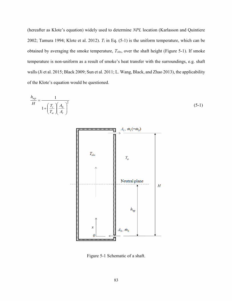
83

(hereafter as Klote’s equation) widely used to determine NPL location (Karlasson and Quintiere

2002; Tamura 1994; Klote et al. 2012). Ti in Eq. (5-1) is the uniform temperature, which can be

obtained by averaging the smoke temperature, Tshx, over the shaft height (Figure 5-1). If smoke

temperature is non-uniform as a result of smoke’s heat transfer with the surroundings, e.g. shaft

walls (Ji et al. 2015; Black 2009; Sun et al. 2011; L. Wang, Black, and Zhao 2013), the applicability

of the Klote’s equation would be questioned.

2

1

1

t

b

a

i

np

A

A

T

TH

h

(5-1)

Figure 5-1 Schematic of a shaft.

84

Black (2009, 2010) considered the effect of temperature distributions on the NPL numerically with

a computer program COntrol of SMOke (COSMO) for specific buildings and found that taller

buildings tend to have lower NPL on a percentage basis relative to building height. Li et al. (2014)

conducted experiments in a 1/3 scale stairwell with three vents located at the top, bottom and mid-

height location, respectively. Temperature distributions were recorded and the NPL was calculated

accordingly. It was found that NPL is closely related to the location of the middle vent, which

directly affected shaft temperature distributions, and the smaller heat release rate results in the

slight lower NPL. Both of these previous studies are based on specific buildings and no general

equation/formulation was provided to improve the Klote’s equation. Although it is always possible

to conduct a numerical simulation or an experiment for a specific building, a general formulation

of NPL, especially in the form of dimensionless parameters similar to the Klote’s equation, would

be preferred.

The distribution of smoke temperature in high-rise shafts is often non-uniform and found to be an

exponential function of relative height (Yang et al. 2013; Qi, Wang, and Zmeureanu 2014a) . From

scaled building model experiments, Li et al. (2014) found that the vertical temperature difference

can be over 55 K for a 12.2-m high shaft. A simplification of the temperature profile as a uniform

temperature may affect the predicted smoke flow rate, pressure distribution, and eventually the

location of NPL. It was found that the uniform temperature assumption may overestimate the

smoke flow rate in a shaft by over 70% (Wang, Black, and Zhao 2013). Qi, Wang, and Zmeureanu

(2014a) developed a mathematical model of smoke movement inside non-adiabatic shafts during

fires, considering non-uniform distribution of temperatures. It was found that the calculated

profiles of smoke temperatures and shaft wall temperatures depend on the temperature attenuation

coefficient, α, a non-dimensional parameter associated with the geometrical and thermal properties

85

of the smoke and the shaft. The NPL can be obtained by the mathematical model however a few

number of iterations are needed, which may not be quite straightforward and practical for actual

designs and analyses in the field of fire protection preferring simpler formulations. The literature

search also shows that there are no existing studies on the evaluation of the applicability of the

uniform temperature assumption to determine the NPL, and the effects of the temperature

distribution and potentially other factors on the NPL location in a high-rise shaft.

Therefore, this study aims to take into account the effects of non-uniform smoke temperature

distribution on the location of NPL in high-rise shafts when compared to the existing model (i.e.

Klote’s equation), which is based on the uniform temperature assumption, and develop a NPL

formulation, e.g. an empirical equation, that do not need iterations when used. Apparently, Klote’s

equation applies to adiabatic shafts where there is no heat transfer between smoke and shaft walls.

Therefore, this study focuses on non-adiabatic shafts and it is based on dimensionless numbers so

it can be generalized to a broad range of cases. First, a method is reported to determine smoke

temperature profile, flow rate and pressure distribution inside non-adiabatic shafts and validated

by the measured data from a 1/3 scale experiment from the literature. Empirical equations for NPL

in terms of associated dimensionless numbers are then developed by regression analysis from the

experimental data. To evaluate the effects of the temperature distribution on NPL, a sensitivity

study of the developed empirical equations is conducted for different shaft bottom temperatures,

ambient temperatures and shaft heights. The applicability and limitations of the existing Klote’s

NPL model are also identified.

5.2. Theory

Because smoke temperature profile affects pressure distribution and consequently NPL location,

we need to find a method to determine the distribution of smoke temperature in a non-adiabatic

86

shaft first. For a buoyancy-driven smoke spread in Figure 5-1, the method in fact needs to solve a

coupled thermal and smoke flow problem. Smoke enters the shaft through the bottom opening and

leaves through the top opening. The corresponding opening areas are Ab and At. To formulate the

coupled equations, we make the following assumptions:

Smoke movement in the shaft is one-dimensional at steady state.

Similar to Klote’s method, smoke temperature at shaft bottom, Tsh0, is higher than Ta.

Specific heat capacity of the smoke, Cp, is constant.

The smoke is assumed to be incompressible and viscous but thermally expansible

satisfying the ideal gas law.

No smoke leaks through shaft walls.

Heat transfer coefficients (either due to convection or radiation) are constant and do not

vary along the height of the shaft.

The effect of wall friction on pressure drop along the shaft height is neglected.

The above coupled thermal airflow problem can be solved by applying mass, heat and mechanical

energy conservation equations developed by the authors (Qi, Wang, and Zmeureanu 2014a). To

avoid repetition, this paper summarizes the final equations of smoke temperature (Eq. 5-2) and

pressure profiles (Eq. 5-9). The average temperature of smoke,shT , wall interior and exterior

surface temperatures, wiT and

woT , are also presented in Eqs. (5-3) ~ (5-5).

HxExpTTTT ashashx )( 0 (5-2)

ExpT

TTTT

a

ashash 11 0 (5-3)

87

Exp

RhT

TTTT

twia

ashawi 1

111 0 (5-4)

Exp

RhT

TTTT

twoa

ashawo 1

11 0

(5-5)

Where

tPRCm

PH

(5-6)

wowi

th

W

hR

11

(5-7)

Heat transfer through the shaft wall is closely related to the thermal resistance between two sides

of the wall, Rt, (Eq. (5-7)), which is determined by heat transfer coefficients on the interior and

exterior shaft wall surfaces (wih and

woh ), as well as thermal conductivity of the wall, k. Both wih

and woh are the effective heat transfer coefficients, which include both convective and radiant heat

transfer portions. The radiant heat transfer depends on many factors, e.g. the geometry of the shaft,

gas composition, gas and wall temperatures. Details about the calculation method of radiant heat

transfer coefficient can be found in the reference Qi, Wang, and Zmeureanu (2014a). A sensitivity

study by Qi, Wang, and Zmeureanu (2014a) also found that the results are not quite sensitive to

the radiant heat transfer portion. Therefore, in this study, only convective heat transfer, hwc, is

considered on shaft wall surfaces, which is also the same as the previous studies did (Sun et al.

2011; Ji et al. 2013). hwc is determined by Eq. (5-8), which combines natural and forced

convections and Cw is 3.08 suggested by Qi, Wang, and Zmeureanu (2014a). wT is the

temperature difference between the average smoke/air and surface temperatures of shaft wall,

which can be calculated using Eqs. (5-3) ~ (5-5).

88

]PrRe)/(037.0,||max[ 3/15/43/1 lkTCh wwwc (5-8)

elxshshx ppp 0 (5-9)

where

0

00

0

)(ln

1

sh

aash

a

ax

elxT

HxExpTTT

RT

Hgpgdxp

(5-10)

Mass flow rate through the top and bottom openings of the shaft is calculated by Eqs. (5-11) and

(5-12).

shHaaHshHtdbt RTpppACmm /)(2 0 (5-11)

002 shaabdb ppACm (5-12)

To obtain the temperature attenuation coefficient, α, temperature profile, Tshx, pressure profile, pshx,

and mass flow rate, m , the above coupled equations need to be solved by iterations. Detailed

calculation steps are shown in Figure 5-2, where bm and Rt are updated in each iteration and taken

into the next iteration until the results converge. However, iterative calculations are not quite

straightforward or practical for designs and analyses in the field of fire protection, which often

relies on simpler formulations, e.g. empirical equations , without the need of iteration, such as the

Klote equation for NPL, the upper-layer gas temperatures equations (McCaffrey, Quintiere, and

Harkleroad 1981), and the equations of plume front locations developed by Cannon and Zukoski

(Ji et al. 2015). Therefore, it would be meaningful to obtain a NPL formulation, e.g. in an empirical

format, that consider non-uniform temperature distribution inside shaft. To achieve this, the first

step is to identify the key physics parameters that can represent the non-uniform temperature

distribution inside shaft. Then based on the key parameters, empirical equations will be developed.

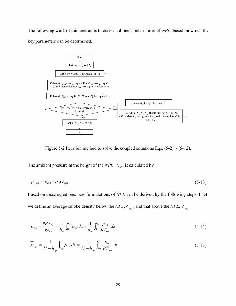
89

The following work of this section is to derive a dimensionless form of NPL, based on which the

key parameters can be determined.

Figure 5-2 Iteration method to solve the coupled equations Eqs. (5-2) ~ (5-12).

The ambient pressure at the height of the NPL, npap , , is calculated by

npaanpa ghpp 0, (5-13)

Based on these equations, new formulations of NPL can be derived by the following steps. First,

we define an average smoke density below the NPL,shl

, and that above the NPL, shu

.

npnpnp

h

shx

a

np

h

shx

npnp

hel

shl dxRT

p

hdx

hgh

p

0

0

0

, 11 (5-14)

H

hshx

a

np

H

hshx

npnpnp

shudx

RT

p

hHdx

hH

011 (5-15)

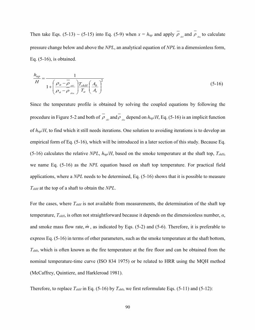
90

Then take Eqs. (5-13) ~ (5-15) into Eq. (5-9) when x = hnp and apply shl

and shu

to calculate

pressure change below and above the NPL, an analytical equation of NPL in a dimensionless form,

Eq. (5-16), is obtained.

2

1

1

t

b

a

shH

a

a

np

A

A

T

TH

h

shu

shl

(5-16)

Since the temperature profile is obtained by solving the coupled equations by following the

procedure in Figure 5-2 and both of shl

andshu

depend on hnp/H, Eq. (5-16) is an implicit function

of hnp/H, to find which it still needs iterations. One solution to avoiding iterations is to develop an

empirical form of Eq. (5-16), which will be introduced in a later section of this study. Because Eq.

(5-16) calculates the relative NPL, hnp/H, based on the smoke temperature at the shaft top, TshH,

we name Eq. (5-16) as the NPL equation based on shaft top temperature. For practical field

applications, where a NPL needs to be determined, Eq. (5-16) shows that it is possible to measure

TshH at the top of a shaft to obtain the NPL.

For the cases, where TshH is not available from measurements, the determination of the shaft top

temperature, TshH, is often not straightforward because it depends on the dimensionless number, α,

and smoke mass flow rate, m , as indicated by Eqs. (5-2) and (5-6). Therefore, it is preferable to

express Eq. (5-16) in terms of other parameters, such as the smoke temperature at the shaft bottom,

Tsh0, which is often known as the fire temperature at the fire floor and can be obtained from the

nominal temperature-time curve (ISO 834 1975) or be related to HRR using the MQH method

(McCaffrey, Quintiere, and Harkleroad 1981).

Therefore, to replace TshH in Eq. (5-16) by Tsh0, we first reformulate Eqs. (5-11) and (5-12):

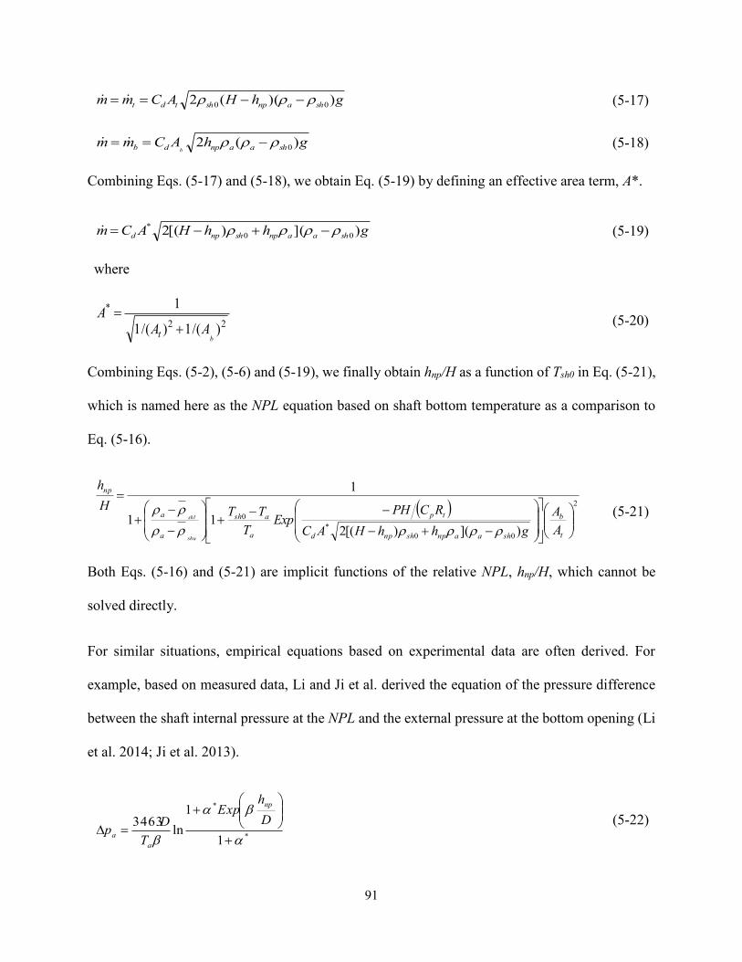
91

ghHACmm shanpshtdt ))((2 00 (5-17)

ghACmm shaanpdb b)(2 0 (5-18)

Combining Eqs. (5-17) and (5-18), we obtain Eq. (5-19) by defining an effective area term, A*.

ghhHACm shaanpshnpd )]()[(2 00

* (5-19)

where

22

*

)/(1)/(1

1

bAA

A

t (5-20)

Combining Eqs. (5-2), (5-6) and (5-19), we finally obtain hnp/H as a function of Tsh0 in Eq. (5-21),

which is named here as the NPL equation based on shaft bottom temperature as a comparison to

Eq. (5-16).

2

00

*

0

)]()[(211

1

t

b

shaanpshnpd

tp

a

ash

a

a

np

A

A

ghhHAC

RCPHExp

T

TTH

h

shu

shl

(5-21)

Both Eqs. (5-16) and (5-21) are implicit functions of the relative NPL, hnp/H, which cannot be

solved directly.

For similar situations, empirical equations based on experimental data are often derived. For

example, based on measured data, Li and Ji et al. derived the equation of the pressure difference

between the shaft internal pressure at the NPL and the external pressure at the bottom opening (Li

et al. 2014; Ji et al. 2013).

*

*

1

1

ln3463

D

hExp

T

Dp

np

a

a (5-22)

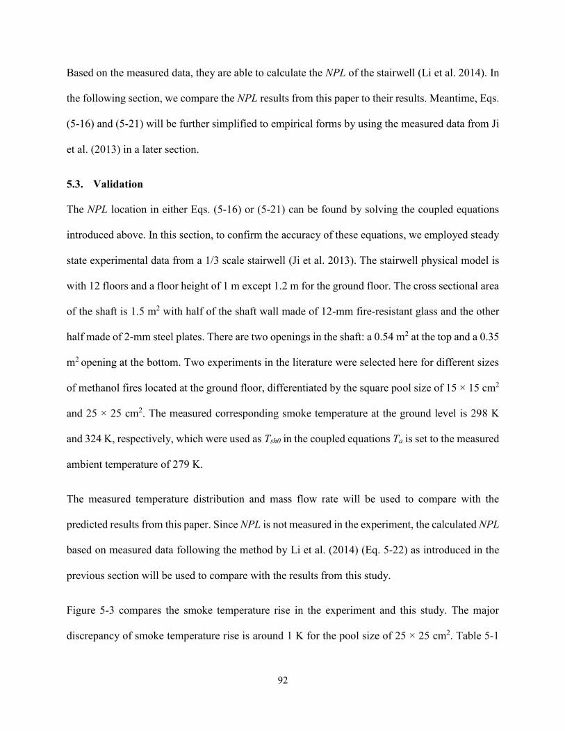
92

Based on the measured data, they are able to calculate the NPL of the stairwell (Li et al. 2014). In

the following section, we compare the NPL results from this paper to their results. Meantime, Eqs.

(5-16) and (5-21) will be further simplified to empirical forms by using the measured data from Ji

et al. (2013) in a later section.

5.3. Validation

The NPL location in either Eqs. (5-16) or (5-21) can be found by solving the coupled equations

introduced above. In this section, to confirm the accuracy of these equations, we employed steady

state experimental data from a 1/3 scale stairwell (Ji et al. 2013). The stairwell physical model is

with 12 floors and a floor height of 1 m except 1.2 m for the ground floor. The cross sectional area

of the shaft is 1.5 m2 with half of the shaft wall made of 12-mm fire-resistant glass and the other

half made of 2-mm steel plates. There are two openings in the shaft: a 0.54 m2 at the top and a 0.35

m2 opening at the bottom. Two experiments in the literature were selected here for different sizes

of methanol fires located at the ground floor, differentiated by the square pool size of 15 × 15 cm2

and 25 × 25 cm2. The measured corresponding smoke temperature at the ground level is 298 K

and 324 K, respectively, which were used as Tsh0 in the coupled equations Ta is set to the measured

ambient temperature of 279 K.

The measured temperature distribution and mass flow rate will be used to compare with the

predicted results from this paper. Since NPL is not measured in the experiment, the calculated NPL

based on measured data following the method by Li et al. (2014) (Eq. 5-22) as introduced in the

previous section will be used to compare with the results from this study.

Figure 5-3 compares the smoke temperature rise in the experiment and this study. The major

discrepancy of smoke temperature rise is around 1 K for the pool size of 25 × 25 cm2. Table 5-1

93

compares the mass flow rates and NPL. The largest relative difference of mass flow rate and NPL

is 13% and 4%, respectively, for the pool size of 15 × 15 cm2. Considering the complexity of the

problem and the relative simplicity of the equations, these discrepancies are not significant and the

predicted results by the coupled equations are acceptable.

Figure 5-3 Comparison of predicted temperature distribution by coupled equations with the

measured data (Ji et al. 2013) for different pool size

Table 5-1 Comparison of predicted mass flow rate and relative NPL by coupled equations with

measured data (Ji et al. 2013) for different pool sizes

Pool size 15×15 cm2 25×25 cm2

Mass flow

rate (kg/s),

ṁ

Ji et al. (2013) 0.252 0.336

This study 0.220 0.328

Relative difference 13% 2%

94

hnp/H

Calculated from Ji et al. (2013) 0.526 0.554

This study 0.507 0.560

Relative difference 4% 1%

5.4. Empirical formulations

According to the validation study, coupled equations that consider the effect of non-uniform

temperature distribution can predict NPL with reasonable accuracy. Meanwhile, to avoid the

iterations needed to solve these coupled equations, this section develops empirical formulations of

NPL that consider the effect of non-uniform temperature distribution based on Eqs. (5-16) and (5-

21).

5.4.1. NPL based on shaft top temperature

The NPL equation based on shaft top temperature, Eq. (5-16), is simplified to Eq. (5-23), a similar

form to the Klote’s equation (Eq. 5-1).

2

1

1

1

1

t

b

N

a

shH

np

A

A

T

TC

H

h

(5-23)

The coefficients C1 and N1 in Eq. (5-23) can be determined by correlation analysis using

experimental data. Here, we use the experiment for the pool sizes of 10 × 10 cm2, 15 × 15 cm2, 20

× 20 cm2, 25 × 25 cm2 and 30 × 30 cm2 from the literature Ji et al. (2013) to obtain the coefficients,

C1 and N1. The measured corresponding smoke temperatures at the bottom opening are 293 K, 298

K, 310 K, 324 K and 346 K, and the temperatures at the top opening are 281 K, 282 K, 286 K, 288

K and 295 K. Figure 5-4 finds that

95

C1 = 2.36 and N1 = -5.13.

The linear correlation coefficient, r, is 0.82, greater than 0.8 indicating a strong correlation (Chan

2003).

Figure 5-4 Correlation for empirical equation based on shaft top temperature.

Different from Klote’s equation, the empirical equation (Eq. 5-23) considers heat transfer between

smoke and shaft wall, which is represented by shaft top temperature, TshH, instead of the uniform

temperature, Ti, in Eq. (5-1). As indicated in Eq. (5-2), TshH is related to smoke inflow temperature,

Tsh0, ambient temperature, Ta, and temperature attenuation coefficient, α, in which the temperature

attenuation coefficient, α, is an index representing smoke temperature distribution inside the shaft

(Qi, Wang, and Zmeureanu 2014a) and it is also a function of overall thermal resistance, Rt, of the

shaft as shown in Eqs. (5-6) and (5-7). A small α indicates a small decrease of the smoke

temperature from bottom to top of the shaft because of large thermal resistance of shaft wall; hence

96

TshH is close to Tsh0. A large α indicates large reduction of the smoke temperature inside the shaft

because of low thermal resistance, and TshH is much lower than Tsh0. Therefore, in Eq. (5-23), heat

transfer through the shaft boundary is closely related to TshH/Ta, which is a dimensionless number

considering non-uniform temperature distribution for a non-adiabatic shaft. Meanwhile, the

obtained constants C1 and N1 are based on the measured data from the literature, which may be

limited and affected by variations of the parameters, e.g. heat transfer coefficient of the shaft wall,

which will be investigated by a sensitivity study of 70 cases in section 5.5 of this paper.

5.4.2. NPL based on shaft bottom temperature

For other scenarios, e.g. when design smoke control systems, TshH is unknown and hard to be

estimated, the empirical equation based on TshH cannot be used. It is necessary to seek an

alternative empirical equation that only uses known parameters, such as the parameters relating to

the shaft structure and design fire. Here, we simplified Eq. (5-21) into Eq. (5-24), where C1 and N1

are the same values as Eq. (5-23), and the coefficient, C2, can be determined by the correlation of

the experimental data.

2

2

0

2*2

01

1

)(11

1

t

b

N

shada

ash

np

A

A

AC

HPCExp

T

TTC

H

h

(5-24)

Based on the measured data from the literature Ji et al. (2013), Figure 5-5 finds that

C2 = 0.0037

with r of 0.81.

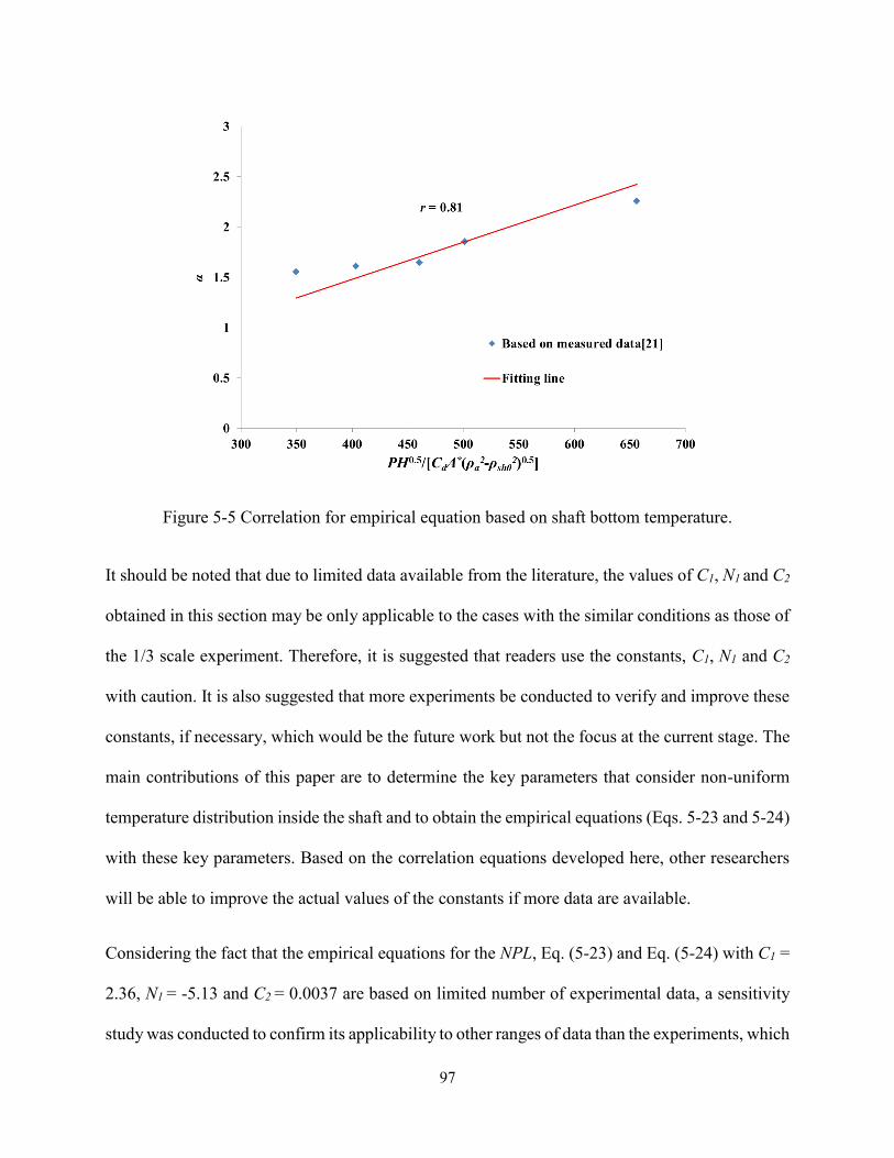
97

Figure 5-5 Correlation for empirical equation based on shaft bottom temperature.

It should be noted that due to limited data available from the literature, the values of C1, N1 and C2

obtained in this section may be only applicable to the cases with the similar conditions as those of

the 1/3 scale experiment. Therefore, it is suggested that readers use the constants, C1, N1 and C2

with caution. It is also suggested that more experiments be conducted to verify and improve these

constants, if necessary, which would be the future work but not the focus at the current stage. The

main contributions of this paper are to determine the key parameters that consider non-uniform

temperature distribution inside the shaft and to obtain the empirical equations (Eqs. 5-23 and 5-24)

with these key parameters. Based on the correlation equations developed here, other researchers

will be able to improve the actual values of the constants if more data are available.

Considering the fact that the empirical equations for the NPL, Eq. (5-23) and Eq. (5-24) with C1 =

2.36, N1 = -5.13 and C2 = 0.0037 are based on limited number of experimental data, a sensitivity

study was conducted to confirm its applicability to other ranges of data than the experiments, which

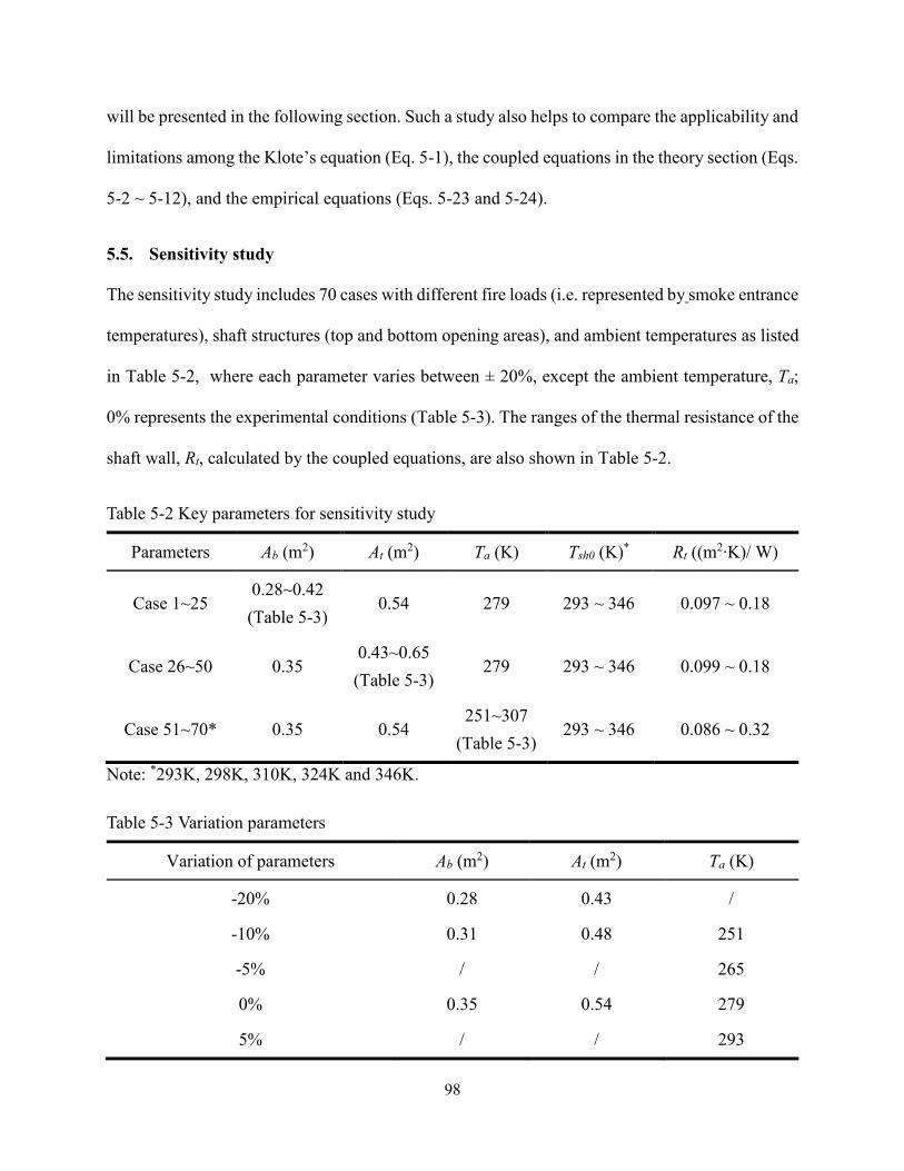
98

will be presented in the following section. Such a study also helps to compare the applicability and

limitations among the Klote’s equation (Eq. 5-1), the coupled equations in the theory section (Eqs.

5-2 ~ 5-12), and the empirical equations (Eqs. 5-23 and 5-24).

5.5. Sensitivity study

The sensitivity study includes 70 cases with different fire loads (i.e. represented by smoke entrance

temperatures), shaft structures (top and bottom opening areas), and ambient temperatures as listed

in Table 5-2, where each parameter varies between ± 20%, except the ambient temperature, Ta;

0% represents the experimental conditions (Table 5-3). The ranges of the thermal resistance of the

shaft wall, Rt, calculated by the coupled equations, are also shown in Table 5-2.

Table 5-2 Key parameters for sensitivity study

Parameters Ab (m2) At (m

2) Ta (K) Tsh0 (K)* Rt ((m2∙K)/ W)

Case 1~25 0.28~0.42

(Table 5-3) 0.54 279 293 ~ 346 0.097 ~ 0.18

Case 26~50 0.35 0.43~0.65

(Table 5-3) 279 293 ~ 346 0.099 ~ 0.18

Case 51~70* 0.35 0.54 251~307

(Table 5-3) 293 ~ 346 0.086 ~ 0.32

Note: *293K, 298K, 310K, 324K and 346K.

Table 5-3 Variation parameters

Variation of parameters Ab (m2) At (m

2) Ta (K)

-20% 0.28 0.43 /

-10% 0.31 0.48 251

-5% / / 265

0% 0.35 0.54 279

5% / / 293

99

10% 0.38 0.59 307

20% 0.42 0.65 /

Figure 5-6 compares the NPL by different methods. For the method based on uniform temperature

distribution assumption (Klote’s equation), TshH is the uniform temperature, Ti, and for the method

of empirical equation based on Tsh0, TshH is calculated by Eq. (5-2). It is found that the predicted

relative NPL by the empirical equations are reasonably close to that of the couple equations. The

predicted relative NPL by the Klote’s equation is also presented in Figure 5-6. Compared to the

results of the coupled equations, the NPL is often overestimated by the Klote’s equation, indicating

that fewer building floors are exposed to smoke and therefore the risk of smoke is underestimated.

Figure 5-6 Comparison of predicted relative NPL.

For a quantitative comparison, NRMSE (Zhao and Wang 2014) in Eq. (5-25) is used. Using the

results from the coupled equations as a baseline, the NRMSE is found to be 6.2%, 6% and 50.1%

for the empirical equations based on TshH, Tsh0, and Klote’s equation, respectively. It shows that

100

the empirical equations perform better than the Klote’s equation for a non-adiabatic shaft during

fires. Considering the thermal resistance of the shaft wall varies from 0.086 to 0.32 (m2∙K)/W as

is shown in Table 5-2, the small values of NRMSE for the empirical equations confirms that the

correlated number C1 and N1 are not strongly dependent on the heat transfer conditions through

the shaft wall for the cases studied in this paper.

2

1

1

2,,

min,max,

11

n

i

icoupiekcoupcoup

PPnPP

NRMSE (5-25)

5.6. Discussion

When the smoke temperature in a shaft is not uniform, such key parameters as fire strength (as

indicated by inflow smoke temperature), shaft opening areas, ambient temperatures, and shaft

heights may have different effects on the NPL location. To better understand the underlying

physics, this section compares the predicted NPL by the empirical equations from this study and

Klote’s equation for different categories of parameters. In the following discussion, except the

parameter that is considered for its effect, other parameters are kept the same as that of the

experiment in the literature Ji et al. (2013).

101

(a)

(b)

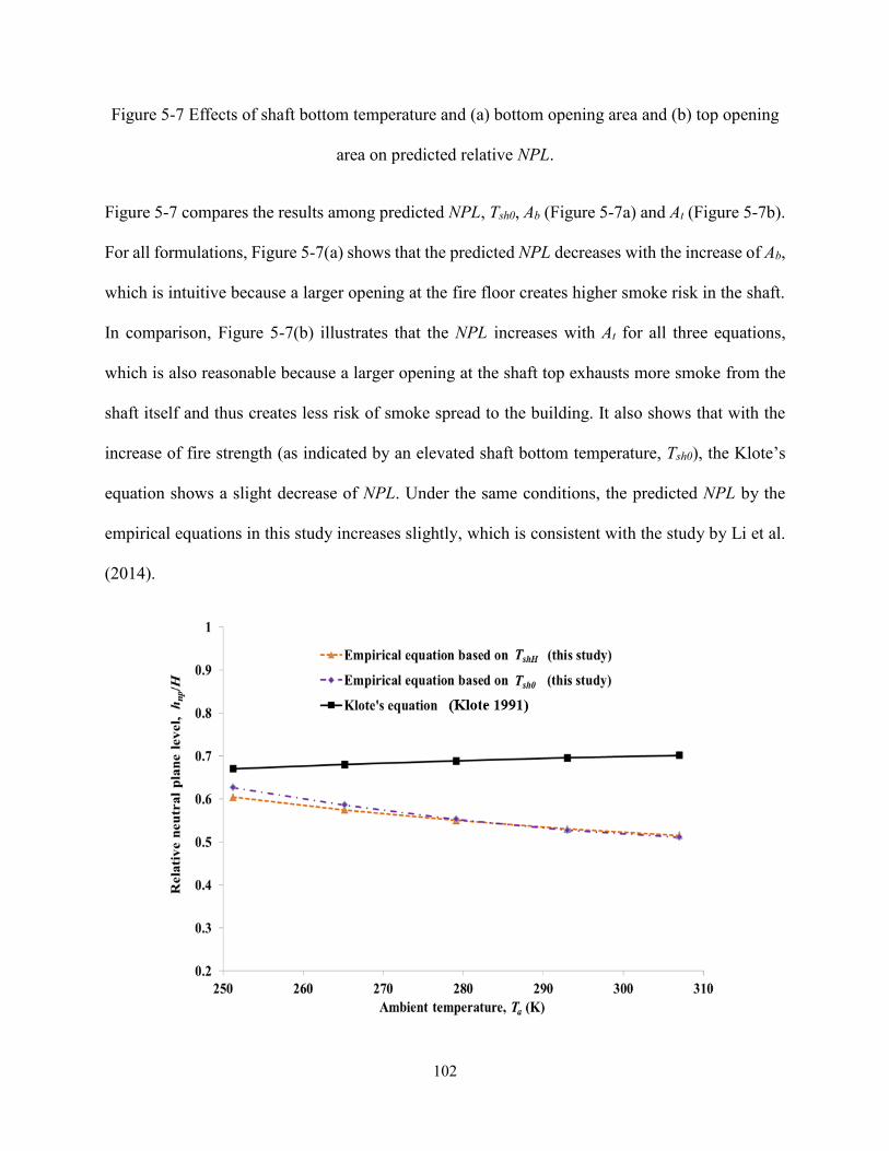
102

Figure 5-7 Effects of shaft bottom temperature and (a) bottom opening area and (b) top opening

area on predicted relative NPL.

Figure 5-7 compares the results among predicted NPL, Tsh0, Ab (Figure 5-7a) and At (Figure 5-7b).

For all formulations, Figure 5-7(a) shows that the predicted NPL decreases with the increase of Ab,

which is intuitive because a larger opening at the fire floor creates higher smoke risk in the shaft.

In comparison, Figure 5-7(b) illustrates that the NPL increases with At for all three equations,

which is also reasonable because a larger opening at the shaft top exhausts more smoke from the

shaft itself and thus creates less risk of smoke spread to the building. It also shows that with the

increase of fire strength (as indicated by an elevated shaft bottom temperature, Tsh0), the Klote’s

equation shows a slight decrease of NPL. Under the same conditions, the predicted NPL by the

empirical equations in this study increases slightly, which is consistent with the study by Li et al.

(2014).

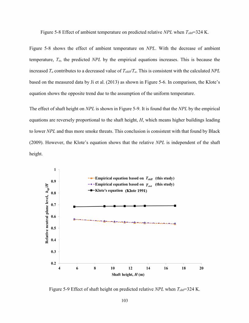
103

Figure 5-8 Effect of ambient temperature on predicted relative NPL when Tsh0=324 K.

Figure 5-8 shows the effect of ambient temperature on NPL. With the decrease of ambient

temperature, Ta, the predicted NPL by the empirical equations increases. This is because the

increased Ta contributes to a decreased value of TshH/Ta. This is consistent with the calculated NPL

based on the measured data by Ji et al. (2013) as shown in Figure 5-6. In comparison, the Klote’s

equation shows the opposite trend due to the assumption of the uniform temperature.

The effect of shaft height on NPL is shown in Figure 5-9. It is found that the NPL by the empirical

equations are reversely proportional to the shaft height, H, which means higher buildings leading

to lower NPL and thus more smoke threats. This conclusion is consistent with that found by Black

(2009). However, the Klote’s equation shows that the relative NPL is independent of the shaft

height.

Figure 5-9 Effect of shaft height on predicted relative NPL when Tsh0=324 K.

104

5.7. Conclusion

To study the effects of non-uniform smoke temperature distribution on the location of NPL, the

coupled equations of temperature distribution, flow rate and pressure distribution were reported

for non-adiabatic shafts and validated by experimental data. Empirical equations based on

dimensionless numbers were developed for NPL through regression analysis. A sensitivity study

of the developed empirical equations was conducted by comparing with the predicted results of

the coupled equations. The applicability and limitations of the conventional NPL model that is

based on uniform temperature assumption (the Klote’s equation) were evaluated by comparing

with the empirical equations. The study reached the following major conclusions:

(1). For non-adiabatic shafts, the effects of non-uniform temperature distribution on NPL should

be considered. The provided case study shows that the uniform temperature assumption leads to

over-estimated NPL, and the relation between shaft bottom/top temperature and NPL predicted

based on this assumption is inconsistent to that of the experiments.

(2). Non-uniform temperature distribution inside of the shaft can be represented by a dimensionless

number, TshH/Ta, which is a ratio of shaft top temperature to ambient temperature. This

dimensionless number is a function of temperature attenuation coefficient, α, which indicates

smoke temperature profile inside the shaft.

(3). The sensitivity study found that the developed empirical equations, which include the

dimensionless number in terms of TshH and Tsh0, can predict NPL accurately. The existing equation

may either underestimate or overestimate the NPL locations.

It is noted that readers should use the obtained constants C1, N1 and C2 of the empirical equations

with caution due to limited data used to develop these constants. The main purpose of this paper

105

is therefore not to provide general applicable values of C1, N1 and C2, but present NPL empirical

equations that can benefit other researchers to understanding the underlying physics regarding the

NPL in high-rise shafts and to developing their own correlations when more data are available.

The limitations of the current study are also noted: the experimental data are limited and the NPL

locations were not directly measured from the experiments. Further studies with more quality

experimental data and measured NPL locations should be done in the future.

106

Chapter 6 Scale Modeling of Steady-state Smoke Spread in Large Vertical

Spaces of High-rise Buildings

Abstract

Large vertical spaces are essential parts of modern high-rise buildings, providing much convenient

and comfortable environment to people. However, driven by stack effect, smoke flows often

spread through the large vertical spaces, which becomes a major challenge for high-rise fire

protections; therefore it is necessary to conduct researches of smoke movement inside the large

vertical spaces. Experimental studies on sub-scaled models play an important role in the fire smoke

research. Froude modeling method is probably the most common approach to design sub-scaled

experiments. However recent studies have found that Froude modeling may not obtain accuracy

temperature on the sub-scaled experiments, especially for the temperature near the building

boundaries where there exists heat transfer between smoke and the boundaries. In this paper, a

new modeling method is developed by deriving dimensionless groups from differential governing

equations that include energy balance and mechanical energy equations for both mechanical and

natural venting systems, in which heat transfer is concerned in the energy balance equation. The

resistance of the inside shaft structure is also concerns by discharge coefficient, Cd. To verify the

new modeling method, experiments were designed on three different size shafts using both Froude

modeling and new modeling methods. The results, including temperature profile, relative neutral

plane level and mass flow rate, are compared between the two modeling methods, and it was found

that the new modeling method can achieve much more accurate results.

6.1. Introduction

In the recent decades, large vertical spaces, elevator shafts, and tall atriums, have been widely used

in high-rise buildings to achieve comfortable environment and energy conservation. For example,

107

the tall atriums applied in the high-rise buildings 1 Bligh Street (Austria) and Palais Royale (India)

could benefit more compartments in the buildings by receiving natural sunlight and make full use

of and natural ventilation to save energy (Wood and Ruba 2013; Colaco, Dravid, and Kasilwal

2012). However, due to the difference of indoor/outdoor densities of buildings, the buoyancy-

driven smoke and toxic flows often spread from fire origins to upper part of the buildings, threating

to people’s lives and properties, and therefore become a major challenge for high-rise fire

protections.

Statistics have shown that about more than 95 % of the upward movement of smoke in typical

high-rise buildings is through the large vertical spaces (Tamura 1994). Numerous studies have

focused on the fire smoke movement inside high-rise large vertical spaces by means of computer

simulation and experiments, in which experiments play an incredible important role. The

experiment is done in the physical world and more realistic (Klote et al. 2012); so the results are

more reliable and computer simulation needs to be verified by it. Since full-size fire experiments

are costly and often unpractical to be conducted in buildings, most of the experimental researches

on smoke movement in high-rise buildings are conducted on sub-scaled physical models. Froude

modeling is probably the most common approach to scale modeling of smoke movement in

buildings, and is widely used for design analysis, verification of CFD simulation and fire

reconstruction. Ding et al. (Ding et al. 2004) studied the possibility of using the same system for

natural ventilation and smoke control in buildings by carrying out CFD simulations of full size 8-

storey building with a solar chimney on top of the atrium. A 1/25 scale model, designed based on

Froude modeling, is developed to validate CFD simulations. To investigate the hot smoky gases

entering an atrium from a fire within an adjacent compartment, Harrison used Froude modeling to

design experiments on 1/10th physical scale model, the results of which were applied to validate

108

CFD simulations (Harrison 2004). Quintiere applied scaling technique to clarify the performance

of a smoke control system which operated in an actual fire incident in a department store atrium.

The scale model results confirmed a design flaw in the smoke control system. The high velocity

inlet air was shown to be responsible for mixing and destratifying the hot smoke in the atrium and

dispersing it throughout the department store (Quintiere and Dillon 2008). To study smoke

movement inside high-rise buildings, 1/3 scaled building model was developed using Froude

modeling, on which extensive researches were conducted on the influence of the staircase

ventilation state on the flow and heat transfer of the heated room on the middle floor (Shi et al.

2014a), the effects of ventilation on the combustion characteristics in the compartment connected

to a stairwell (Ji et al. 2016).

However, several studies found that sub-scaled experiments using Froude modeling may not obtain

accurate temperature. Carey compared temperatures at different locations between a full

compartments and a 1/8 scaled compartments designed based on Froude modeling. It was found

that the accuracy of the model does vary based on the distance from the fire. Due to heat transfer

between the gas and the boundary, the temperatures measured near the boundaries are not as

accurate as the temperatures measured closer to the fire. For the measuring location 5.1 cm below

the ceiling and 5.76 m away from the fire of 250 kW gas burner, temperature rise of full size

model is 40°C but the difference between full model and 1/8 scaled model is up to 20°C (Allison

C. Carey 2010). Chow carried out experiments of natural smoke filling process on both full-scale

atrium and a 1/26.5 scale atrium. The experiments were designed according to Froude modeling.

However, it was observed that there are quite large deviations between the temperatures measured

in the scale model and the full-size atrium. Therefore, they suggested that the scaling law for

temperature requires further examination (Chow and Lo 2008). The large deviation is probably

109

caused by the negligence of heat transfer between the smoke/gas and the boundaries. During a

high-rise fires, fire smoke temperature can be an order of magnitude higher than surrounding air

at the bottom of large vertical spaces and drop quickly at the higher floor due to the heat exchange

between the fire smoke and the boundaries (Qi, Wang, and Zmeureanu 2014a; Qi, Wang, and

Zmeureanu 2015). Therefore it is necessary to consider the heat transfers when sub-scale the large

vertical spaces during fires.

Smoke spread in high-rise vertical spaces is often either driven naturally by buoyancy due to the

temperature difference of the smoke and the ambient, and/or mechanically by air moving devices,

such as fans. This paper investigated both ventilation means starting by examining the differential

forms of the governing conservation equations including heat balance equation, mechanical energy

equation and continuity equation. Compared to previous work of scaling analysis, this study did

not start the analysis with general and full-form partial differential equations but instead use a

simplified form of analytical solutions to the heat and mass transfer in high-rise shafts. The new

method helps to provide a better and more straightforward route to developing the required

dimensionless groups suitable for the current specific problem. To verify the new scaling model,

experiments were conducted in three shaft models with scale ratio of 1:1/3:1/4 and different

materials for both mechanical and natural movement of the fire smoke. The performance of the

similarity of the new model was then compared to the traditional Froude modeling method.

6.2. Governing equations and dimensionless groups

A scaling method is based on dimensionless groups/dimensionless variables (Munson et al. 2009).

To obtain the dimensionless groups, governing equations that describe the phenomenon of interests

are expressed in terms of dimensionless variables in this section.

110

Smoke movement inside the large vertical spaces can be modeled using one-dimensional forms of

the governing equations at steady state (Qi, Wang, and Zmeureanu 2015; Qi, Wang, and

Zmeureanu 2014b; Ji et al. 2013). In this paper, a shaft in Fig. 6-1 is employed to represent a

typical large vertical space in high-rise building. At the top of the shaft, a fan is used to exhaust

smoke from the shaft when mechanically-driven smoke spread system applies, while during

naturally-driven, the exhaust fan is replaced by an opening. The following sections, section 6.2.1,

and 6.2.2, report the derived dimensionless equations and groups for mechanically and naturally

driven, respectively.

Figure 6-1 Schematic of a high-rise shaft during fires

6.2.1. Mechanical smoke venting

The dimensional governing equations of heat balance, and mechanical energy balance along the

vertical direction of the shaft, and at the bottom of the shaft are listed in Eqs. (6-1) ~ (6-3),

respectively.

Heat balance equation:

111

0)(

t

ashxshxP

R

PdxTTdTCm (6-1)

Mechanical energy balance equation along the height of shaft:

0 gdxdp shxshx (6-2)

Mechanical energy equation at the bottom opening of shaft:

02

2 dvdp a (6-3)

To nondimensionalize the above equations, the following dimensionless parameters are defined.

Dimensionless temperature:

shx

af

ashxshx

TT

TTT

(6-4)

Dimensionless height or relative height:

H

xx

(6-5)

Dimensionless smoke velocity:

db Cv

vv

/

(6-6)

where vb is the velocity of air at bottom opening.

Dimensionless pressure:

gH

ppp

a

a

0

(6-7)

Based on the Buckingham Π theorem, Eqs (6-1) ~ (6-3) can then be converted to their

dimensionless forms accordingly.

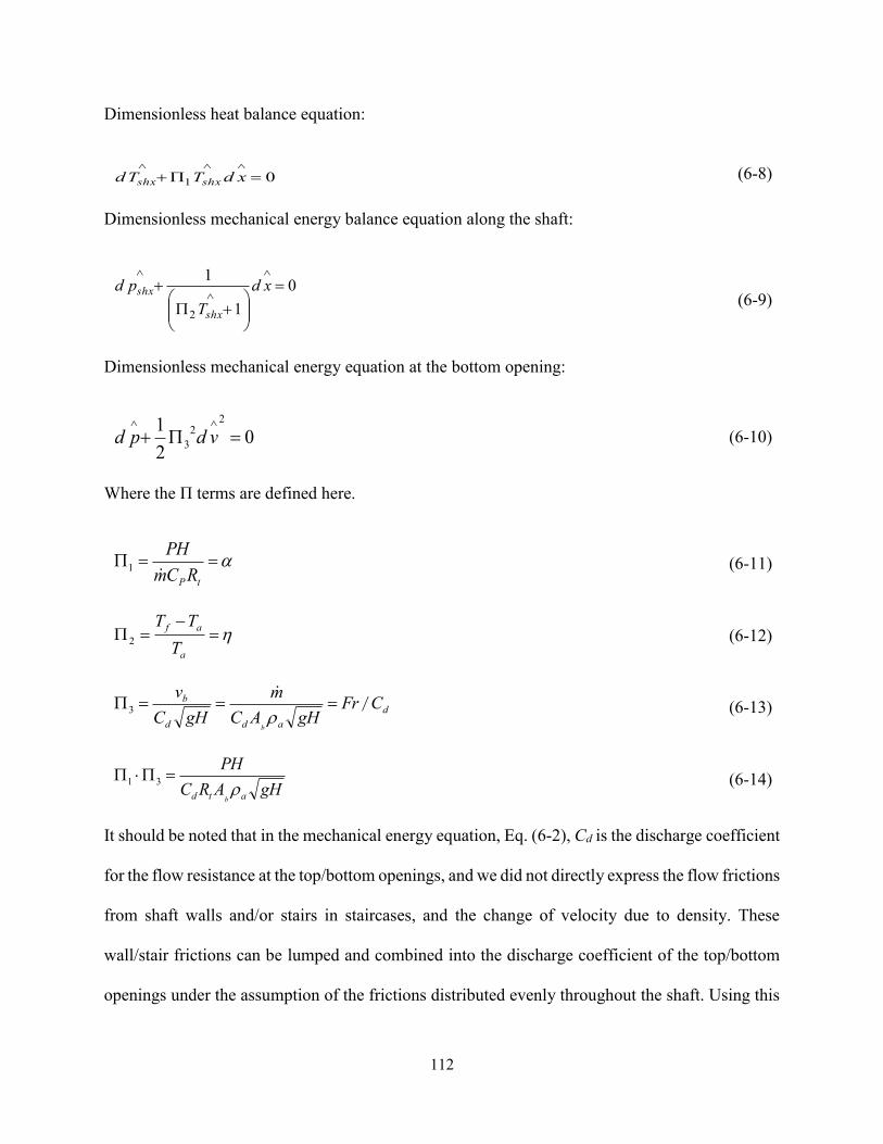
112

Dimensionless heat balance equation:

01

xdTTd shxshx (6-8)

Dimensionless mechanical energy balance equation along the shaft:

0

1

1

2

xd

T

pd

shx

shx (6-9)

Dimensionless mechanical energy equation at the bottom opening:

02

1 22

3

vdpd (6-10)

Where the Π terms are defined here.

tP RCm

PH

1 (6-11)

a

af

T

TT2 (6-12)

d

add

b CFrgHAC

m

gHC

v

b

/

3 (6-13)

gHARC

PH

atd b

31 (6-14)

It should be noted that in the mechanical energy equation, Eq. (6-2), Cd is the discharge coefficient

for the flow resistance at the top/bottom openings, and we did not directly express the flow frictions

from shaft walls and/or stairs in staircases, and the change of velocity due to density. These

wall/stair frictions can be lumped and combined into the discharge coefficient of the top/bottom

openings under the assumption of the frictions distributed evenly throughout the shaft. Using this

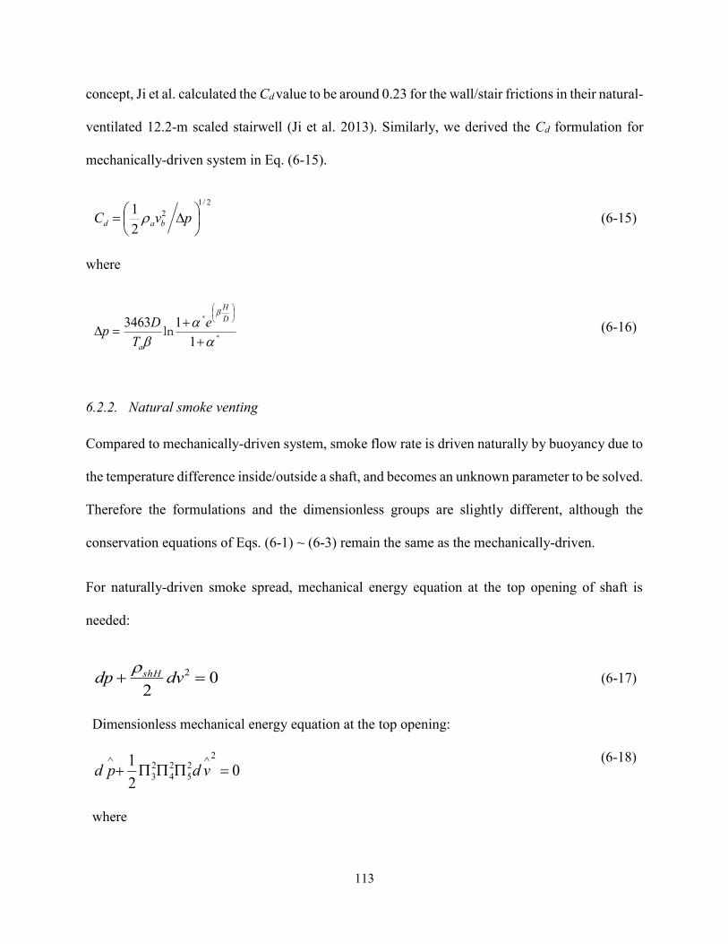
113

concept, Ji et al. calculated the Cd value to be around 0.23 for the wall/stair frictions in their natural-

ventilated 12.2-m scaled stairwell (Ji et al. 2013). Similarly, we derived the Cd formulation for

mechanically-driven system in Eq. (6-15).

2/1

2

2

1

pvC bad (6-15)

where

*

*

ln

1

13463 D

H

a

e

T

Dp (6-16)

6.2.2. Natural smoke venting

Compared to mechanically-driven system, smoke flow rate is driven naturally by buoyancy due to

the temperature difference inside/outside a shaft, and becomes an unknown parameter to be solved.

Therefore the formulations and the dimensionless groups are slightly different, although the

conservation equations of Eqs. (6-1) ~ (6-3) remain the same as the mechanically-driven.

For naturally-driven smoke spread, mechanical energy equation at the top opening of shaft is

needed:

02

2 dvdp shH (6-17)

Dimensionless mechanical energy equation at the top opening:

02

1 22

5

2

4

2

3

vdpd

(6-18)

where

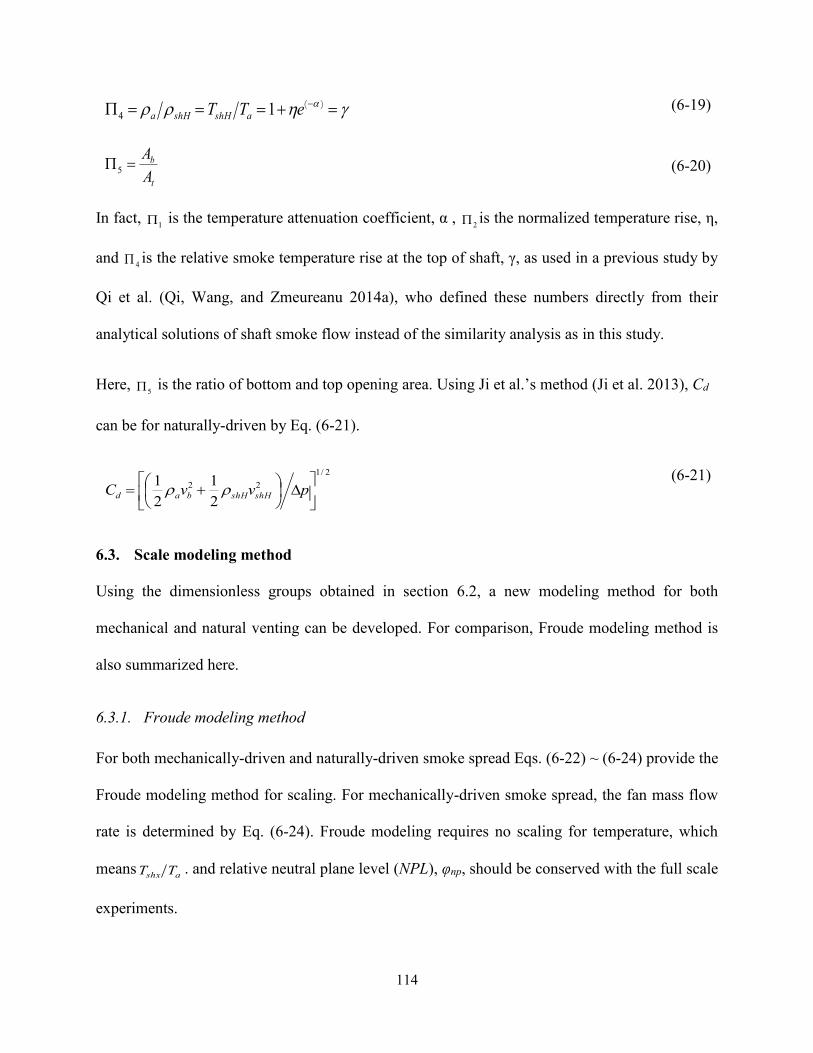
114

)(eTT ashHshHa 14 (6-19)

t

b

A

A5 (6-20)

In fact, 1 is the temperature attenuation coefficient, α ,

2 is the normalized temperature rise, η,

and 4 is the relative smoke temperature rise at the top of shaft, γ, as used in a previous study by

Qi et al. (Qi, Wang, and Zmeureanu 2014a), who defined these numbers directly from their

analytical solutions of shaft smoke flow instead of the similarity analysis as in this study.

Here, 5 is the ratio of bottom and top opening area. Using Ji et al.’s method (Ji et al. 2013), Cd

can be for naturally-driven by Eq. (6-21).

2/1

22

2

1

2

1

pvvC shHshHbad

(6-21)

6.3. Scale modeling method

Using the dimensionless groups obtained in section 6.2, a new modeling method for both

mechanical and natural venting can be developed. For comparison, Froude modeling method is

also summarized here.

6.3.1. Froude modeling method

For both mechanically-driven and naturally-driven smoke spread Eqs. (6-22) ~ (6-24) provide the

Froude modeling method for scaling. For mechanically-driven smoke spread, the fan mass flow

rate is determined by Eq. (6-24). Froude modeling requires no scaling for temperature, which

meansashx TT . and relative neutral plane level (NPL), φnp, should be conserved with the full scale

experiments.

115

Geometry similarity:

f

mfm

H

Hxx (6-22)

Heat release rate:

f

f

mm E

H

HE

25/

(6-23)

Mass flow rate:

2/5

2/5

f

mfm

H

Hmm (6-24)

6.3.2. New modeling method

Mechanical venting

As mentioned earlier, the issue with the Froude modeling is that heat transfer is not properly

modeled so temperature similarity cannot be maintained as expected: the scaled temperature is

often significantly different from the full-size value. Therefore, one of the major objectives here

for the new scaling method is to maintain the same

shxT and

p , 1 , 2 , 3 need to be maintained

according to Eqs. (6-8) ~ (6-10).

Since 31 is only decided by the features of the shaft and ambient air density as shown in Eq.

(6-15) and is easier to be calculated without considering the mass flow rate, m , we use 31

instead of 1 . As a result parameters, 31 ,

2 and3 , need to be conserved. The new scaling

method on the basis of 31 ,2 and

3 for mechanically-driven smoke spread is shown in Eqs.

(6-25) ~ (6-28), in which Eqs. (6-26) ~ (6-28) are derived from 31 (Eq. 6-14), 2 (Eq. 6-12)

and 3 (Eq. 6-13) respectively. The new modeling method indicates that as long as Eqs. (6-25) ~

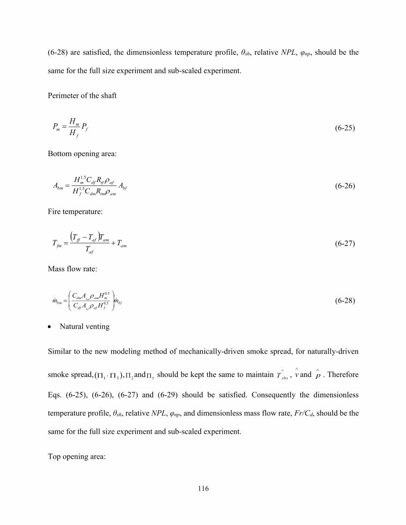
116

(6-28) are satisfied, the dimensionless temperature profile, θsh, relative NPL, φnp, should be the

same for the full size experiment and sub-scaled experiment.

Perimeter of the shaft

f

f

mm P

H

HP (6-25)

Bottom opening area:

bf

amtmdmf

aftfdfm

bm ARCH

RCHA

5.1

5.1

(6-26)

Fire temperature:

am

af

amafff

fm TT

TTTT

(6-27)

Mass flow rate:

bf

fafdf

mamdm

bm mHAC

HACm

bf

bm

5.0

5.0

(6-28)

Natural venting

Similar to the new modeling method of mechanically-driven smoke spread, for naturally-driven

smoke spread, 31 ,2 and

5 should be kept the same to maintain

shxT ,

v and

p . Therefore

Eqs. (6-25), (6-26), (6-27) and (6-29) should be satisfied. Consequently the dimensionless

temperature profile, θsh, relative NPL, φnp, and dimensionless mass flow rate, Fr/Cd, should be the

same for the full size experiment and sub-scaled experiment.

Top opening area:

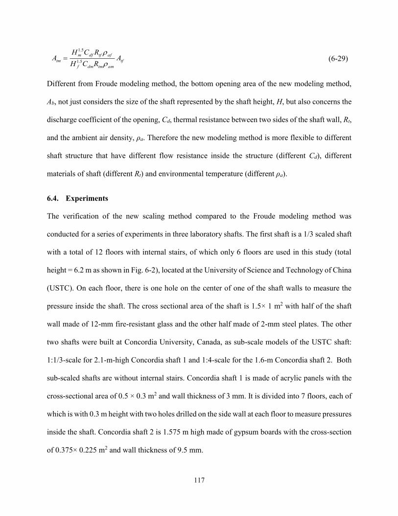
117

tf

amtmdmf

aftfdfm

tm ARCH

RCHA

5.1

5.1

(6-29)

Different from Froude modeling method, the bottom opening area of the new modeling method,

Ab, not just considers the size of the shaft represented by the shaft height, H, but also concerns the

discharge coefficient of the opening, Cd, thermal resistance between two sides of the shaft wall, Rt,

and the ambient air density, ρa. Therefore the new modeling method is more flexible to different

shaft structure that have different flow resistance inside the structure (different Cd), different

materials of shaft (different Rt) and environmental temperature (different ρa).

6.4. Experiments

The verification of the new scaling method compared to the Froude modeling method was

conducted for a series of experiments in three laboratory shafts. The first shaft is a 1/3 scaled shaft

with a total of 12 floors with internal stairs, of which only 6 floors are used in this study (total

height = 6.2 m as shown in Fig. 6-2), located at the University of Science and Technology of China

(USTC). On each floor, there is one hole on the center of one of the shaft walls to measure the

pressure inside the shaft. The cross sectional area of the shaft is 1.5× 1 m2 with half of the shaft

wall made of 12-mm fire-resistant glass and the other half made of 2-mm steel plates. The other

two shafts were built at Concordia University, Canada, as sub-scale models of the USTC shaft:

1:1/3-scale for 2.1-m-high Concordia shaft 1 and 1:4-scale for the 1.6-m Concordia shaft 2. Both

sub-scaled shafts are without internal stairs. Concordia shaft 1 is made of acrylic panels with the

cross-sectional area of 0.5 × 0.3 m2 and wall thickness of 3 mm. It is divided into 7 floors, each of

which is with 0.3 m height with two holes drilled on the side wall at each floor to measure pressures

inside the shaft. Concordia shaft 2 is 1.575 m high made of gypsum boards with the cross-section

of 0.375× 0.225 m2 and wall thickness of 9.5 mm.

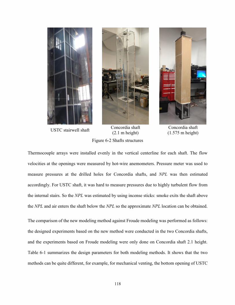
118

USTC stairwell shaft Concordia shaft

(2.1 m height)

Concordia shaft

(1.575 m height)

Figure 6-2 Shafts structures

Thermocouple arrays were installed evenly in the vertical centerline for each shaft. The flow

velocities at the openings were measured by hot-wire anemometers. Pressure meter was used to

measure pressures at the drilled holes for Concordia shafts, and NPL was then estimated

accordingly. For USTC shaft, it was hard to measure pressures due to highly turbulent flow from

the internal stairs. So the NPL was estimated by using incense sticks: smoke exits the shaft above

the NPL and air enters the shaft below the NPL so the approximate NPL location can be obtained.

The comparison of the new modeling method against Froude modeling was performed as follows:

the designed experiments based on the new method were conducted in the two Concordia shafts,

and the experiments based on Froude modeling were only done on Concordia shaft 2.1 height.

Table 6-1 summarizes the design parameters for both modeling methods. It shows that the two

methods can be quite different, for example, for mechanical venting, the bottom opening of USTC

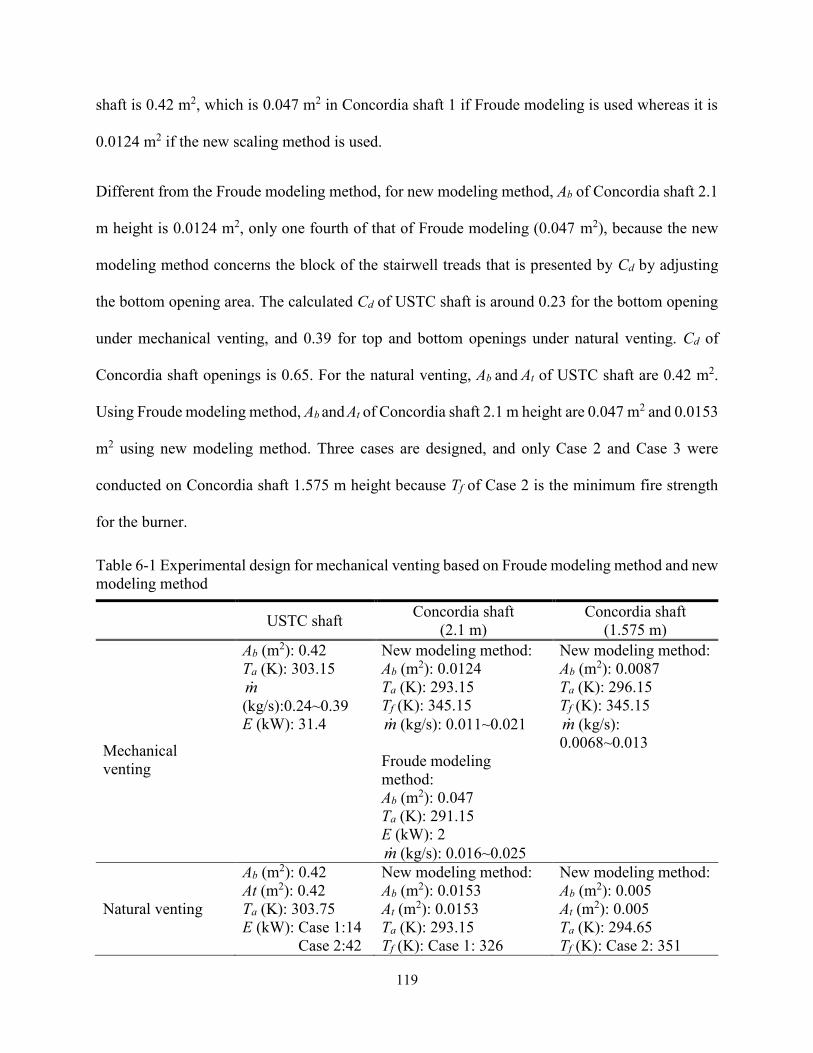
119

shaft is 0.42 m2, which is 0.047 m2 in Concordia shaft 1 if Froude modeling is used whereas it is

0.0124 m2 if the new scaling method is used.

Different from the Froude modeling method, for new modeling method, Ab of Concordia shaft 2.1

m height is 0.0124 m2, only one fourth of that of Froude modeling (0.047 m2), because the new

modeling method concerns the block of the stairwell treads that is presented by Cd by adjusting

the bottom opening area. The calculated Cd of USTC shaft is around 0.23 for the bottom opening

under mechanical venting, and 0.39 for top and bottom openings under natural venting. Cd of

Concordia shaft openings is 0.65. For the natural venting, Ab and At of USTC shaft are 0.42 m2.

Using Froude modeling method, Ab and At of Concordia shaft 2.1 m height are 0.047 m2 and 0.0153

m2 using new modeling method. Three cases are designed, and only Case 2 and Case 3 were

conducted on Concordia shaft 1.575 m height because Tf of Case 2 is the minimum fire strength

for the burner.

Table 6-1 Experimental design for mechanical venting based on Froude modeling method and new

modeling method

USTC shaft Concordia shaft

(2.1 m)

Concordia shaft

(1.575 m)

Mechanical

venting

Ab (m2): 0.42

Ta (K): 303.15

m(kg/s):0.24~0.39

E (kW): 31.4

New modeling method:

Ab (m2): 0.0124

Ta (K): 293.15

Tf (K): 345.15

m (kg/s): 0.011~0.021

Froude modeling

method:

Ab (m2): 0.047

Ta (K): 291.15

E (kW): 2

m (kg/s): 0.016~0.025

New modeling method:

Ab (m2): 0.0087

Ta (K): 296.15

Tf (K): 345.15

m (kg/s):

0.0068~0.013

Natural venting

Ab (m2): 0.42

At (m2): 0.42

Ta (K): 303.75

E (kW): Case 1:14

Case 2:42

New modeling method:

Ab (m2): 0.0153

At (m2): 0.0153

Ta (K): 293.15

Tf (K): Case 1: 326

New modeling method:

Ab (m2): 0.005

At (m2): 0.005

Ta (K): 294.65

Tf (K): Case 2: 351

120

Case 3:73

Case 2: 343

Case 3: 372

Froude modeling method

Ab (m2): 0.047

At (m2): 0.047

Ta (K): 303.75

E (kW): Case 1:0.93

Case 2:2.8

Case 3:4.9

Case 3: 382

6.5. Results and discussion

For the three different shafts, temperature profiles, θsh, and relative NPL, φnp, are compared for

mechanical venting and temperature profiles, θsh, mass flow rate, ṁ and relative NPL, φnp, for

natural venting. For a quantitative comparison, Normalized Root Mean Square Error (NRMSE)

(Zhao and Wang 2014) in Eq. (6-30) is used to explain the temperature difference between USTC

shaft and Concordia shaft with 2.1 m height. Using the experimental data of the USTC shaft as a

baseline. P1 is the temperature of USTC shaft and P2 is the temperature of Concordia shaft with

2.1 m height. The less value of NRMSE the better performance of scale modeling method is.

2

1

1

2

21

11

11

n

i

ii PPnPP

NRMSE ,,

min,max,

(6-30)

6.5.1. Mechanical smoke venting

Temperature profiles of cases with Fr/Cd around 0.38 and 0.42 are compared in Fig. 6-3.

Temperature profile is presented by the value of θsh for the new modeling method and Tshx/Ta for

Froude modeling method. It can be observed that Tshx/Ta of Concordia shaft is much higher than

that of USTC shaft by Froude modeling method, because the thermal resistance between two sides

of the shaft wall for Concordia shaft is larger than that of USTC shaft but it is neglected in the

Froude modeling. Using the new modeling method that considers heat transfer between smoke and

121

the shaft wall and interior structure resistance, the temperature distribution of Concordia shaft is

much closer to USTC shaft. The values of NRMSE decrease significantly, from 254 % to 17 % and

from 248% to 23% when the new modeling method applied.

(a) Fr/Cd=0.38, Froude modeling method (b) Fr/Cd=0.38, New modeling method

(c) Fr/Cd=0.42, Froude modeling method (d) Fr/Cd=0.42, New modeling method

Figure 6-3 Comparison of temperature profiles

Figure 6-4 compares the measured relative NPL of the two scaling method, in which the new

modeling method performs better than Froude modeling method. Using Froude modeling, for the

experiments conducted on USTC shaft, the relative NPL, φnp, increases dramatically, from 0.32 to

0.95, when ṁ/H5/2 increases slightly from 0.003 to 0.004 kg/m5/2. However, for the experiments

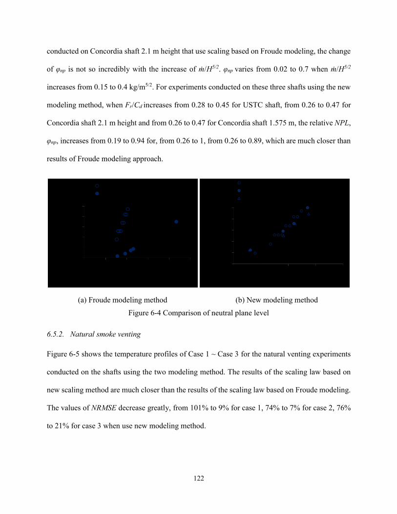
122

conducted on Concordia shaft 2.1 m height that use scaling based on Froude modeling, the change

of φnp is not so incredibly with the increase of ṁ/H5/2. φnp varies from 0.02 to 0.7 when ṁ/H5/2

increases from 0.15 to 0.4 kg/m5/2. For experiments conducted on these three shafts using the new

modeling method, when Fr/Cd increases from 0.28 to 0.45 for USTC shaft, from 0.26 to 0.47 for

Concordia shaft 2.1 m height and from 0.26 to 0.47 for Concordia shaft 1.575 m, the relative NPL,

φnp, increases from 0.19 to 0.94 for, from 0.26 to 1, from 0.26 to 0.89, which are much closer than

results of Froude modeling approach.

(a) Froude modeling method (b) New modeling method

Figure 6-4 Comparison of neutral plane level

6.5.2. Natural smoke venting

Figure 6-5 shows the temperature profiles of Case 1 ~ Case 3 for the natural venting experiments

conducted on the shafts using the two modeling method. The results of the scaling law based on

new scaling method are much closer than the results of the scaling law based on Froude modeling.

The values of NRMSE decrease greatly, from 101% to 9% for case 1, 74% to 7% for case 2, 76%

to 21% for case 3 when use new modeling method.

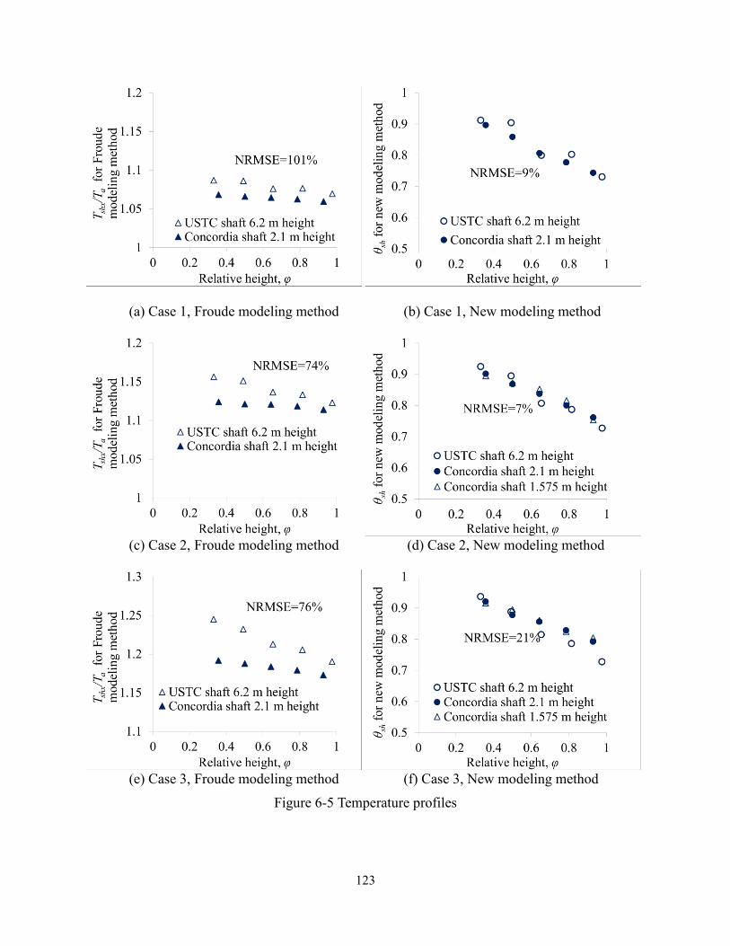
123

(a) Case 1, Froude modeling method (b) Case 1, New modeling method

(c) Case 2, Froude modeling method (d) Case 2, New modeling method

(e) Case 3, Froude modeling method (f) Case 3, New modeling method

Figure 6-5 Temperature profiles

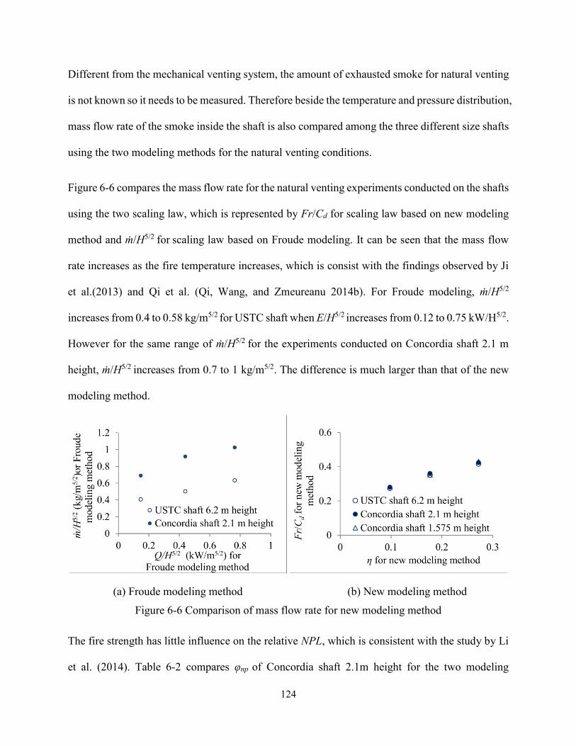
124

Different from the mechanical venting system, the amount of exhausted smoke for natural venting

is not known so it needs to be measured. Therefore beside the temperature and pressure distribution,

mass flow rate of the smoke inside the shaft is also compared among the three different size shafts

using the two modeling methods for the natural venting conditions.

Figure 6-6 compares the mass flow rate for the natural venting experiments conducted on the shafts

using the two scaling law, which is represented by Fr/Cd for scaling law based on new modeling

method and ṁ/H5/2 for scaling law based on Froude modeling. It can be seen that the mass flow

rate increases as the fire temperature increases, which is consist with the findings observed by Ji

et al.(2013) and Qi et al. (Qi, Wang, and Zmeureanu 2014b). For Froude modeling, ṁ/H5/2

increases from 0.4 to 0.58 kg/m5/2 for USTC shaft when E/H5/2 increases from 0.12 to 0.75 kW/H5/2.

However for the same range of ṁ/H5/2 for the experiments conducted on Concordia shaft 2.1 m

height, ṁ/H5/2 increases from 0.7 to 1 kg/m5/2. The difference is much larger than that of the new

modeling method.

(a) Froude modeling method (b) New modeling method

Figure 6-6 Comparison of mass flow rate for new modeling method

The fire strength has little influence on the relative NPL, which is consistent with the study by Li

et al. (2014). Table 6-2 compares φnp of Concordia shaft 2.1m height for the two modeling

125

method .With the increase of fire strength, φnp is around 0.57±0.1 for USTC shaft. When use the

new modeling method, φnp is around 0.46±0.05 for the Concordia shaft. It is much better than

Froude modeling, for which φnp is around 0.75±0.16.

Table 6-2 Measured relative neutral plane level

New modeling

method

Froude modeling

method

USTC shaft 0.57 ± 0.1 / /

Concordia shaft 2.1m height / 0.46 ± 0.05 0.75± 0.16

6.6. Conclusion

Smoke tends to spread from lower part of the high-rise buildings to higher part through large

vertical spaces, which becomes a major challenge for fire protection. The sub-scaled experiment

is an essential practical approach to study smoke movement inside buildings compared with full-

size experiments which are costly. However, there lack of modeling method to sub-scale the large

vertical spaces that needs to consider heat transfer between smoke and the boundaries. This paper

presents a new modeling method to scale smoke movement in large vertical spaces in high-rise

buildings during fires, which is derived from differential equations including energy balance and

mechanical and energy equations. Heat transfer between smoke and the boundaries and the

resistant effect of inside structure, e.g. stairs, on the vertical spreading flow are considered in the

new modeling method, which differs from Froude modeling.

To verify the accuracy of this new modeling method, a series of experiments were designed and

conducted on three different size shafts for both mechanical venting and natural venting. The

results were also compared with Froude modeling methods. This study reached the following

major conclusions:

126

(1) By using the discharge coefficient, Cd, to express the inside structure resistance of the shaft,

the shaft with inside structure, like shaft with stairs, could be sub-scaled as the shaft without

inside structure, which is simpler to model.

(2) By considering heat transfer between smoke and the boundaries and inside structure resistance,

the new modeling method could achieve more accurate results than Froude modeling method.

127

Chapter 7 Modeling Smoke Movement in High-rise Shafts by a Multizone

Airflow and Energy Network Program

The contents of this chapter are published in “Dahai Qi, Liangzhu Wang, Radu Zmeureanu. 2015.

Modeling Smoke Movement in Shafts during High-Rise Fires by a Multizone Airflow and Energy

Network Program. ASHRAE Transactions 121 (2)”. The contents are slightly modified.

Abstract

Multizone airflow network programs are increasingly used to study smoke movement during fires

in buildings. Multizone programs often do not solve energy conservation equation so temperatures

of rooms/zones need to be specified. The lack of energy model limits the capability of a multizone

program for modeling building smoke movement, especially in shafts, where temperature

distribution is often unknown. This paper introduces a multizone program with an added energy

equation, CONTAM97R, with the focus of its application to simulations of smoke movement,

especially in shafts of high-rise buildings. First, CONTAM97R was validated by experimental data

from a 1/3 scale building stairwell under fires, and verified by an analytical model of high-rise

fires. The program is then used to model a 16-storey building with a fire located at the first floor.

To model the building shaft by CONTAM97R, we proposed and compared two zoning methods,

Floor Zoning Strategy (FZS) and Adaptive Zoning Strategy (AZS), when the shaft is with and

without air infiltrations. It shows that the accuracy of FZS is inversely related to a dimensionless

parameter, the temperature attenuation coefficient, α, but can be improved by increasing the

number of zones dividing the shaft until the results do not depend on zone numbers. Compared to

FZS, AZS obtains results of similar level of accuracy but with fewer zones for the simulations.

128

7.1. Introduction

A high-rise building is often defined as a building with the height more than 23 m (NFPA 101

2012). As one of the key indicators of modernization, high-rise buildings bring many conveniences

for people’s lives in populated cities. During the design and construction of a high-rise building,

engineers and architects must cope with a variety of security and life safety issues, among which

the management of fire smoke movement is one of the most important tasks. Most of the fire-

related deaths in buildings are caused by inhalation of smoke. In the United States, fire smoke

accounts for approximately 75% of victims in building fires (Beitel, Wakelin, and Beyler 2000).

For high-rises, the situation is worsened when fire smoke migrates long distances from the room

of fire origin to the rest of a building under stack effect through vertical structures (Shi et al. 2014a;

Li et al. 2014), e.g. stair and elevator shafts, light wells, and ventilation ducts, where often little

flow resistance is encountered. Therefore a good knowledge of smoke movement, especially in

vertical shafts, is extremely important for the design of high-rise fire smoke control systems.

A multizone airflow network program (hereafter multizone program) is often used to study smoke

movement during fires in buildings (Black 2009; Klote et al. 2012; Bae, Shin, and Ryou 2014). A

whole-building multizone analysis of smoke movement usually only needs a few minutes or even

seconds (Wang and Chen 2008). Developed by the US National Institute of Standards and

Technology, CONTAM (Walton and Dols 2013) is the multizone program for building fire smoke

analysis as suggested by the Handbook of Smoke Control Engineering (Klote et al. 2012). Miller

et al. conducted CONTAM simulations to study smoke controls by shaft pressurization in high-

rise buildings. CONTAM was employed as a major model for the investigation of the fire smoke

movement in the World Trade Center (WTC) on 9/11/2001 (Ferreira and Strege 2005). However,

CONTAM does not solve the energy conservation equation so temperature in each zone has to be

129

specified by users. Therefore, in the studies of Miller et al., a single value of temperature averaged

over the entire shaft height was used as the input in CONTAM (Miller and Beasley 2009; Miller

2011). Due to the lack of energy model, inappropriate temperature inputs may lead to simulation

errors, especially for the scenarios of buoyancy-driven smoke movement, where smoke

temperatures are often unknown beforehand (Ferreira and Strege 2005). Wang, Black, and Zhao

(2013) simulated smoke movement in a 40-storey building using CONTAM and compared the

results to another multizone-type program added with energy model, COntrol of SMOke (COSMO)

(Black 2010). They found that the accuracy of temperature profile in the shaft is the key to the

quality of the prediction. Inaccurately specified temperatures will lead to errors in excess of 70%.

The addition of the thermal analysis capability to CONTAM thus becomes quite necessary.

There have been some previous efforts to add an energy model to CONTAM (Tang and Glicksman

2005; McDowell et al. 2003; Gu 2011), many of which have not yet resulted in a final product.

Among them, CONTAM97R (Axley 2011; Wang, Dols, and Emmerich 2012) is probably the most

completed one, which was firstly developed in 1997, and later validated by Axley et al. (2002) for

modeling of naturally ventilated buildings. However, there have been scarce studies of modeling

building fire smoke movement by CONTAM97R, although CONTAM, the sister program without

an energy model, has been increasingly used for building smoke analysis as noted previously. One

of the main challenges is how to divide a long shaft in several zones in a multizone program, so-

called “zoning strategy”: specifically, how many zones should be used and how to distribute the

zones in a vertical shaft while each zone is considered to have a uniform temperature under the

well-mixed assumption (Wang, Dols, and Emmerich 2012). One of the most common zoning

strategies may be to assign one zone for the shaft section of each floor (e.g. a shaft of a 16-story

building will be divided into 16 zones) or to further divide each shaft zone into several vertical

130

sub-zones (hereafter, Floor Zoning Strategy) as what have been done in the previous studies

(Miller and Beasley 2009;Wang, Black, and Zhao 2013). However, because each zone is assumed

to have a single temperature, how many zones a shaft are divided will directly affect the predicted

temperature distribution, and consequently smoke flow rates and pressure profiles. Floor Zoning

Strategy (FZS) thus needs to be further evaluated, and if necessary a better zoning strategy should

be suggested.

The purpose of this paper is to use CONTAM97R for the simulations of smoke movement in high-

rise shafts during fires. First, the energy model in CONTAM97R is briefly introduced.

CONTAM97R is then validated by the experimental data from a 1/3 scaled building model under

fires, and verified by an analytical model in the literature (Qi, Wang, and Zmeureanu 2014a). We

then used CONTAM97R to model the smoke movement in a 16-storey building with a fire located

at the first floor when the shaft is with and without air infiltrations. Using the analytical model of

the 16-story building as a baseline, we evaluated two zoning strategies to divide the vertical shaft

into multiple sub-zones, namely, FZS and an alternative, Adaptive Zoning Strategy (AZS). The

conclusions and experiences from this paper can be applied to other studies of using similar

multizone network programs for modeling fire smoke movement in high-rise buildings.

7.2. Fundamentals

Energy model in CONTAM97R

The energy model in CONTAM97R can be illustrated by an example of two rooms in Figure 7-1,

where zone i and zone j are connected through path ij, surrounded by the ambient zone, zone a.

For zone i, the energy conservation equation for the zone thermal node can be written as:

131

k

iwkiwkwki

j

ijipi

a

aiapaiipi

TTAhEmTCmTCdt

mTCd (7-1)

The convective heat transfer coefficient, hwk, is determined by the temperature difference between

the interior wall surface and the indoor air. The conductive heat transfer through the wall k from

the wall thermal node ki to kj is considered by the Fourier’s Law in Equation 7-2, and solved by a

1-D finite difference method.

dy

dTkq (7-2)

Equations 7-1 and 7-2 show the equations solved by the CONTAM97R modules of the zone

thermal node and the wall thermal node, respectively. During an energy and airflow network

analysis, the program solves the mass balance equation of the airflow network (the equation is not

provided here but can be found from the CONTAM user guide (Walton and Dols 2013) first to

obtain zone pressures and airflows under given initial zone and wall temperatures. Then the zone

and the wall thermal node modules are solved sequentially to update the temperature values. Two

approaches are provided for the integration of this thermal airflow problem, “Ping-Pong” and

“Onion” (Zhai, Johnson, and Krarti 2011). The Onion approach requires the convergence of both

thermal and airflow analyses at the same time step whereas the Ping-Pong approach solves each

module only once at each time step so it needs shorter time step than the Onion approach. The

details of these two approaches can be found in previous studies (Hensen 1999; Sahlin 2003), so

they are not included here. All the simulations in this paper used the Ping-Pong approach to obtain

final results at steady state.

132

Figure 7-1 Schematic of the energy model in CONTAM97R

Analytical model of high-rise fire smoke movement

The validity of a computer program, such as CONTAM97R, should be better verified by

comparing the predicted results to experimental data. High-quality experimental data of full-size

high-rise fires are scarce in the literature partly due to the fact that full-scale field measurements

are challenging and costly. Therefore, in the later section of this paper, we try to validate

CONTAM97R by an experimental study in a reduced-scaled building model and an analytical

model of a high-rise building when the data for a full-scale building are needed. This section

summarizes the fundamentals of the analytical model (Qi, Wang, and Zmeureanu 2014a). For a

building with a fire, e.g. the one located at the first floor as shown in Figure 7-2, the analytical

model was developed under the following assumptions:

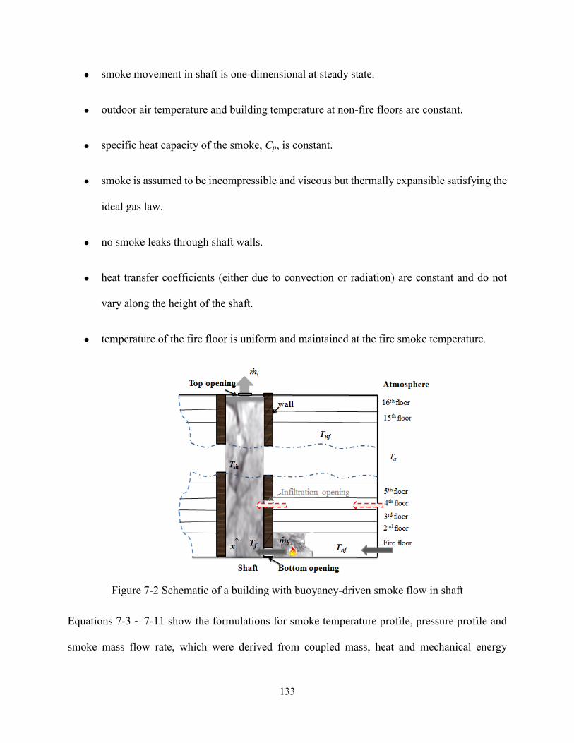
133

smoke movement in shaft is one-dimensional at steady state.

outdoor air temperature and building temperature at non-fire floors are constant.

specific heat capacity of the smoke, Cp, is constant.

smoke is assumed to be incompressible and viscous but thermally expansible satisfying the

ideal gas law.

no smoke leaks through shaft walls.

heat transfer coefficients (either due to convection or radiation) are constant and do not

vary along the height of the shaft.

temperature of the fire floor is uniform and maintained at the fire smoke temperature.

Figure 7-2 Schematic of a building with buoyancy-driven smoke flow in shaft

Equations 7-3 ~ 7-11 show the formulations for smoke temperature profile, pressure profile and

smoke mass flow rate, which were derived from coupled mass, heat and mechanical energy

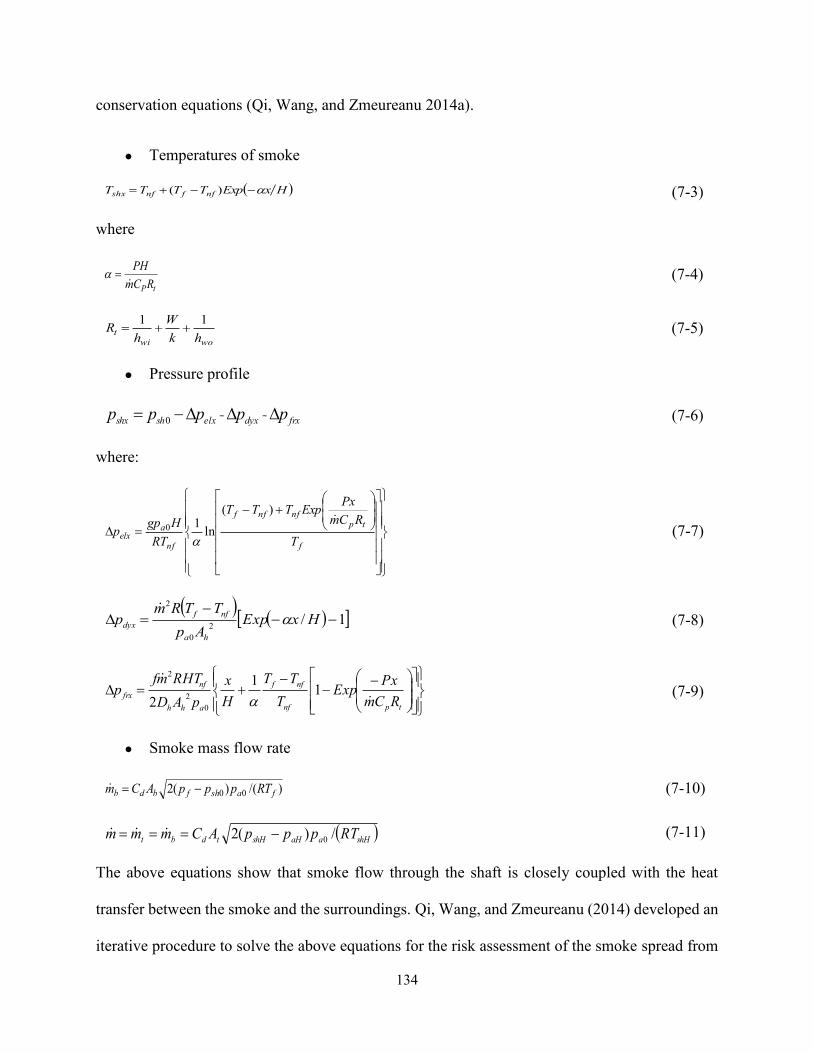
134

conservation equations (Qi, Wang, and Zmeureanu 2014a).

Temperatures of smoke

HxExpTTTT nffnfshx )( (7-3)

where

tPRCm

PH

(7-4)

wowi

thk

W

hR

11

(7-5)

Pressure profile

frxdyxelxshshx ppppp --0 (7-6)

where:

f

tpnfnff

nf

aelx

T

RCm

PxExpTTT

RT

Hgpp

)(

ln10

(7-7)

1/

2

0

2

HxExpAp

TTRmp

ha

nff

dyx

(7-8)

tpnf

nff

ahh

nf

frxRCm

PxExp

T

TT

H

x

pAD

RHTmfp

1

1

2 0

2

2

(7-9)

Smoke mass flow rate

)/()(2 00 fashfbdb RTpppACm

(7-10)

shHaaHshHtdbt RTpppACmmm /)(2 0

(7-11)

The above equations show that smoke flow through the shaft is closely coupled with the heat

transfer between the smoke and the surroundings. Qi, Wang, and Zmeureanu (2014) developed an

iterative procedure to solve the above equations for the risk assessment of the smoke spread from

135

the fire floor to higher floors. The temperature profiles of smoke and shaft wall are both shown to

be exponential functions of the temperature attenuation coefficient, α, defined by Equation 7-4.

The accuracy of the analytical model was confirmed by the comparison to numerical simulations

and measured data in the literature. The details were not provided here to avoid repetition but can

be found in their paper (Qi, Wang, and Zmeureanu 2014a).

7.3. Validation by reduced-scale building model

To validate CONTAM97R in modeling of high-rise shafts during fires, we employed the

experimental data from a 1/3 scale stairwell (Ji et al. 2013) in the literature, and the calculated

results based on the analytical model in the previous section (Qi, Wang, and Zmeureanu 2014a).

The 1/3 scale stairwell model has 12 floors with a floor height of 1 m (3.28 ft) except 1.2 m (3.94

ft) for the ground floor, and with a cross sectional area of 1.5 m (4.92 ft) × 1.0 m (3.28 ft) (L × W).

Two sides of the stairwell model are made from 12-mm (0.03937 ft) fire-resistant glass and the

other two sides are from 2-mm (0.006562 ft) thick steel plates. The experimental data at steady

state were selected here for two square pool sizes of 20 cm (0.66 ft) × 20 cm (0.66 ft) and 30 cm

(0.98 ft) × 30 cm (0.98 ft) with the Methanol fire sources located at the height of 0.6 m (1.969 ft).

The measured corresponding smoke temperature at the ground level is 310 K (98.3 0F) and 346 K

(163.1 0F), respectively. The non-fire floor temperature and outdoor temperature were measured

to be 279.15 K (42.8 0F).

Given the above information, a CONTAM97R model of the reduced-scale building model was

created with one zone assigned to each floor following the mostly common approach of FZS so a

total of 12 zones were created for the shaft. Due to the small thinness of the shaft wall which has

good heat conduction with outside atmosphere, in this particular case, the heat loss to the boundary

is simplified as a convective process and the conductive heat transfer is ignored (Sun et al. 2011)

136

in the analytical model and CONTAM97R. Figure 7-3 and Table 7-1 compare the gas temperature

rise and mass flow rates among the experiment, CONTAM97R and the analytical model. The

temperature predictions of CONTAM97R, analytical model and experimental results are almost

identical. CONTAM97R overestimates the smoke mass flow rate with a difference of less than 7%

and the analytical model underestimates the flow rate with 7.7% for the 30 cm (0.98 ft) × 30 cm

(0.98 ft) fire. Considering the complexities and uncertainties of the experiments, these

discrepancies are not quite significant and CONTAM97R predictions are considered acceptable.

Meanwhile, the comparison in this section also shows the validity of the analytical model, which

will be used as a baseline in the later section when experimental data of full-size buildings are not

available.

As mentioned previously, different zoning strategies may affect the predictions of temperatures,

smoke mass flow rates and pressure profiles. FZS is shown to be acceptable in this specific

experiment but may become inapplicable in other cases, which will be discussed in the following

section.

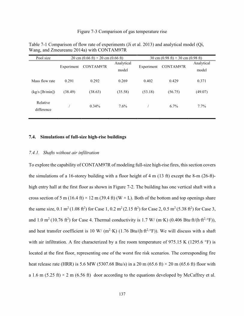
137

Figure 7-3 Comparison of gas temperature rise

Table 7-1 Comparison of flow rate of experiments (Ji et al. 2013) and analytical model (Qi,

Wang, and Zmeureanu 2014a) with CONTAM97R

Pool size 20 cm (0.66 ft) × 20 cm (0.66 ft) 30 cm (0.98 ft) × 30 cm (0.98 ft)

Experiment CONTAM97R Analytical

model Experiment CONTAM97R

Analytical

model

Mass flow rate

(kg/s [lb/min])

0.291

(38.49)

0.292

(38.63)

0.269

(35.58)

0.402

(53.18)

0.429

(56.75)

0.371

(49.07)

Relative

difference / 0.34% 7.6% / 6.7% 7.7%

7.4. Simulations of full-size high-rise buildings

7.4.1. Shafts without air infiltration

To explore the capability of CONTAM97R of modeling full-size high-rise fires, this section covers

the simulations of a 16-storey building with a floor height of 4 m (13 ft) except the 8-m (26-ft)-

high entry hall at the first floor as shown in Figure 7-2. The building has one vertical shaft with a

cross section of 5 m (16.4 ft) × 12 m (39.4 ft) (W × L). Both of the bottom and top openings share

the same size, 0.1 m2 (1.08 ft2) for Case 1, 0.2 m2 (2.15 ft2) for Case 2, 0.5 m2 (5.38 ft2) for Case 3,

and 1.0 m2 (10.76 ft2) for Case 4. Thermal conductivity is 1.7 W/ (m·K) (0.406 Btu∙ft/(h∙ft2∙°F)),

and heat transfer coefficient is 10 W/ (m2·K) (1.76 Btu/(h∙ft2∙°F)). We will discuss with a shaft

with air infiltration. A fire characterized by a fire room temperature of 975.15 K (1295.6 °F) is

located at the first floor, representing one of the worst fire risk scenarios. The corresponding fire

heat release rate (HRR) is 5.6 MW (5307.68 Btu/s) in a 20 m (65.6 ft) × 20 m (65.6 ft) floor with

a 1.6 m (5.25 ft) × 2 m (6.56 ft) door according to the equations developed by McCaffrey et al.

138

for relating HRR and the fire room temperature (Karlasson and Quintiere 2002). During the fire,

the fire smoke would enter the shaft and spread across all higher floors. The ambient is considered

with an outdoor temperature of 253.15 K (-4 °F) under no wind condition. Since the analytical

model is for steady state, we run a transient simulation with a time step of 10 minutes till the steady

state is reached, which is confirmed when the variation of the predicted temperature in the shaft is

less than a threshold value of 1×10-4 K (0.56×10-4 °F). The simulations were run on a desktop

computer with a 2.40-GHz processor and 4GB memory.

Note that since there are no experimental data available for the modeled full-size building, we use

the calculated results of the analytical model as the baseline for the comparison. In the following

sections, we compare two zoning strategies for the shaft of the modeled building.

Floor Zoning Strategy (FZS)

One of the most common methods of dividing the shaft is probably to assign one zone for each

floor or to further divide each floor zone into several sub-zones with equal size (Black 2009; Klote

et al. 2012). For this so-called “Floor Zoning Strategy”, we first studied the case of one zone

assigned for each floor, which results in a total of 16 zones for the modeled shaft. Note that for

simplicity without loss of generality, each non-fire floor is assumed to be one open space and

modeled as a single zone as what was often done by the previous studies (Wang, Black, and Zhao

2013; Black 2010).

Figure 7-4 compare the predicted smoke temperatures and mass flow rates to the results of the

analytical model for all the four cases with different opening sizes. For a given value of α, Figure

7-4(a) shows that the calculated temperatures are all functions of the height in the vertical shaft.

The predicted smoke mass flow rates agree better with the analytical model than the temperature

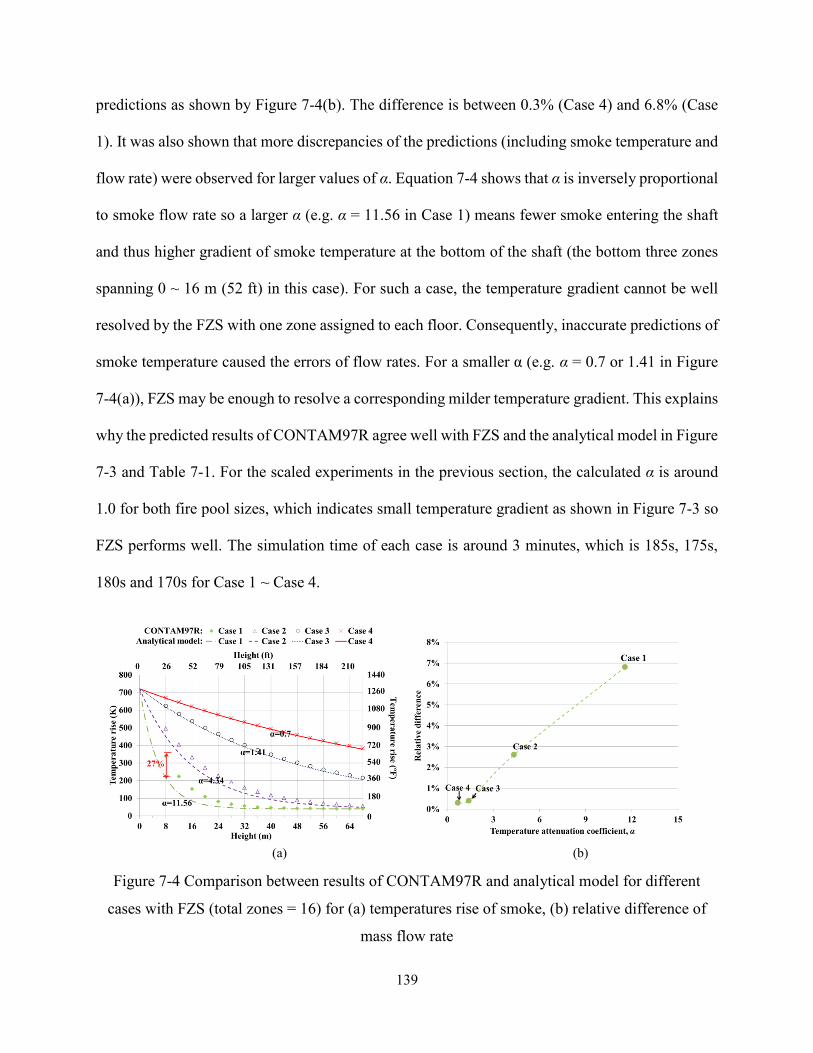
139

predictions as shown by Figure 7-4(b). The difference is between 0.3% (Case 4) and 6.8% (Case

1). It was also shown that more discrepancies of the predictions (including smoke temperature and

flow rate) were observed for larger values of α. Equation 7-4 shows that α is inversely proportional

to smoke flow rate so a larger α (e.g. α = 11.56 in Case 1) means fewer smoke entering the shaft

and thus higher gradient of smoke temperature at the bottom of the shaft (the bottom three zones

spanning 0 ~ 16 m (52 ft) in this case). For such a case, the temperature gradient cannot be well

resolved by the FZS with one zone assigned to each floor. Consequently, inaccurate predictions of

smoke temperature caused the errors of flow rates. For a smaller α (e.g. α = 0.7 or 1.41 in Figure

7-4(a)), FZS may be enough to resolve a corresponding milder temperature gradient. This explains

why the predicted results of CONTAM97R agree well with FZS and the analytical model in Figure

7-3 and Table 7-1. For the scaled experiments in the previous section, the calculated α is around

1.0 for both fire pool sizes, which indicates small temperature gradient as shown in Figure 7-3 so

FZS performs well. The simulation time of each case is around 3 minutes, which is 185s, 175s,

180s and 170s for Case 1 ~ Case 4.

(a) (b)

Figure 7-4 Comparison between results of CONTAM97R and analytical model for different

cases with FZS (total zones = 16) for (a) temperatures rise of smoke, (b) relative difference of

mass flow rate

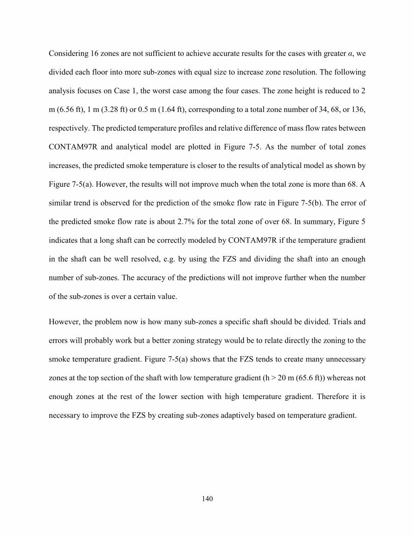
140

Considering 16 zones are not sufficient to achieve accurate results for the cases with greater α, we

divided each floor into more sub-zones with equal size to increase zone resolution. The following

analysis focuses on Case 1, the worst case among the four cases. The zone height is reduced to 2

m (6.56 ft), 1 m (3.28 ft) or 0.5 m (1.64 ft), corresponding to a total zone number of 34, 68, or 136,

respectively. The predicted temperature profiles and relative difference of mass flow rates between

CONTAM97R and analytical model are plotted in Figure 7-5. As the number of total zones

increases, the predicted smoke temperature is closer to the results of analytical model as shown by

Figure 7-5(a). However, the results will not improve much when the total zone is more than 68. A

similar trend is observed for the prediction of the smoke flow rate in Figure 7-5(b). The error of

the predicted smoke flow rate is about 2.7% for the total zone of over 68. In summary, Figure 5

indicates that a long shaft can be correctly modeled by CONTAM97R if the temperature gradient

in the shaft can be well resolved, e.g. by using the FZS and dividing the shaft into an enough

number of sub-zones. The accuracy of the predictions will not improve further when the number

of the sub-zones is over a certain value.

However, the problem now is how many sub-zones a specific shaft should be divided. Trials and

errors will probably work but a better zoning strategy would be to relate directly the zoning to the

smoke temperature gradient. Figure 7-5(a) shows that the FZS tends to create many unnecessary

zones at the top section of the shaft with low temperature gradient (h > 20 m (65.6 ft)) whereas not

enough zones at the rest of the lower section with high temperature gradient. Therefore it is

necessary to improve the FZS by creating sub-zones adaptively based on temperature gradient.

141

(a) (b)

Figure 7-5 Effects of zone numbers on the (a) predicted smoke temperature and (b) relative

difference of predicted mass flow rate between CONTAM97R and analytical model for shafts

without infiltration in Case 1

Adaptive Zoning Strategy (AZS)

We proposed an Adaptive Zoning Strategy (AZS), which limits temperature difference between

two neighboring zones by a temperature constraint, β, defined by Equation (7-14). θshx is the

dimensionless smoke temperature defined by Equation 10 (Qi, Wang, and Zmeureanu 2014a). For

a specific temperature constraint, the height of each zone, hi, can be obtained by Equation 7-12.

)( ihxshshx , 0<β<1 (7-12)

where

H

xExp

TT

TT

nff

nfshxshx

(7-13)

H

HxExphi

/1ln (7-14)

The temperature constraint in the above equations restricts the temperature variation between two

neighbor zones. For a section of the shaft with high temperature gradient, a smaller β indicates less

temperature variation allowed between zones and thus results in more sub-zones created. For a

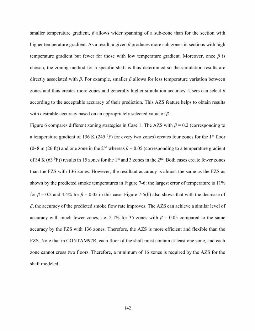
142

smaller temperature gradient, β allows wider spanning of a sub-zone than for the section with

higher temperature gradient. As a result, a given β produces more sub-zones in sections with high

temperature gradient but fewer for those with low temperature gradient. Moreover, once β is

chosen, the zoning method for a specific shaft is thus determined so the simulation results are

directly associated with β. For example, smaller β allows for less temperature variation between

zones and thus creates more zones and generally higher simulation accuracy. Users can select β

according to the acceptable accuracy of their prediction. This AZS feature helps to obtain results

with desirable accuracy based on an appropriately selected value of β.

Figure 6 compares different zoning strategies in Case 1. The AZS with β = 0.2 (corresponding to

a temperature gradient of 136 K (245 0F) for every two zones) creates four zones for the 1st floor

(0~8 m (26 ft)) and one zone in the 2nd whereas β = 0.05 (corresponding to a temperature gradient

of 34 K (63 0F)) results in 15 zones for the 1st and 3 zones in the 2nd. Both cases create fewer zones

than the FZS with 136 zones. However, the resultant accuracy is almost the same as the FZS as

shown by the predicted smoke temperatures in Figure 7-6: the largest error of temperature is 11%

for β = 0.2 and 4.4% for β = 0.05 in this case. Figure 7-5(b) also shows that with the decrease of

β, the accuracy of the predicted smoke flow rate improves. The AZS can achieve a similar level of

accuracy with much fewer zones, i.e. 2.1% for 35 zones with β = 0.05 compared to the same

accuracy by the FZS with 136 zones. Therefore, the AZS is more efficient and flexible than the

FZS. Note that in CONTAM97R, each floor of the shaft must contain at least one zone, and each

zone cannot cross two floors. Therefore, a minimum of 16 zones is required by the AZS for the

shaft modeled.

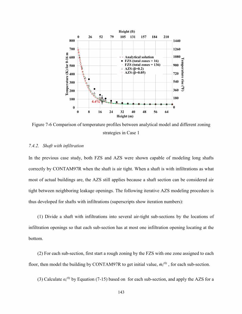
143

Figure 7-6 Comparison of temperature profiles between analytical model and different zoning

strategies in Case 1

7.4.2. Shaft with infiltration

In the previous case study, both FZS and AZS were shown capable of modeling long shafts

correctly by CONTAM97R when the shaft is air tight. When a shaft is with infiltrations as what

most of actual buildings are, the AZS still applies because a shaft section can be considered air

tight between neighboring leakage openings. The following iterative AZS modeling procedure is

thus developed for shafts with infiltrations (superscripts show iteration numbers):

(1) Divide a shaft with infiltrations into several air-tight sub-sections by the locations of

infiltration openings so that each sub-section has at most one infiltration opening locating at the

bottom.

(2) For each sub-section, first start a rough zoning by the FZS with one zone assigned to each

floor, then model the building by CONTAM97R to get initial value, ṁi(0) , for each sub-section.

(3) Calculate αi(0) by Equation (7-15) based on for each sub-section, and apply the AZS for a

144

selected β to get an updated ṁi(1) for each sub-section.

(4) For each sub-section, if | ṁi (1)– ṁi

(0)|/ ṁi (1) is over a convergence threshold, return to the

step (3) by updating ṁi(0)= ṁi

(1) till the desirable accuracy is obtained.

The above procedure is demonstrated by a case study of the same building with an infiltration

opening located at the bottom of the fourth floor as shown in Figure 7-2. The opening is with the

size of 0.1 m2 (1.08 ft2) and modeled by the orifice equation with discharge coefficient of 0.6 and

flow exponent of 0.5 (Walton and Dols 2013). All the other settings are kept the same as the

previous case of Case 1. As a baseline for comparison, the FZS with the total zone of 153 is applied

to obtain the results independent of zone numbers.

Figure 7-7 shows the shaft zoning for the AZS with β = 0.05 compared to the FZS with 153 zones.

There exist two regions with high temperature gradients: one at the 1st floor near the smoke entry

location and the other at the 4th floor with air infiltration. The AZS adaptively creates fine zone

resolutions at both locations but with only a total of 48 zones in the whole shaft compared to the

FZS with 153 zones.

145

Figure 7-7 Shaft zoning by the FZS with 153 zones and the AZS with β=0.05 for the shaft with

an infiltration opening at the 4th floor in the 16-storey building

Table 7-2 Comparison of mass flow rate (kg/s [lb/min]) of the 16-storey building with an

infiltration opening at the 4th floor.

FZS

(total zone = 153)

AZS (β=0.05)

First iteration Second iteration

Sub-section 0 (0)-16 m (52 ft) 0.447

(59.1)

0.441

(58.3)

0.440

(58.2)

Sub-section 16 (52 ft)-68 m (223 ft) 0.826

(109.3)

0.829

(109.7)

0.829

(109.7)

Table 7-2 lists the predicted mass flow rate of each zoning method. The ASZ only needs two

iterations to reach a convergence threshold of 0.1% for the mass flow rate. The calculated flow

rate is pretty close to the baseline value in the FZS. Similarly, the predicted temperature and

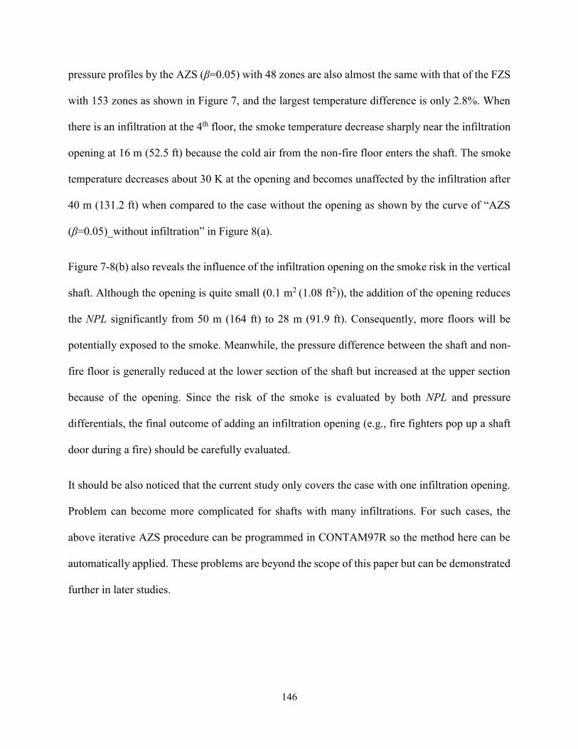
146

pressure profiles by the AZS (β=0.05) with 48 zones are also almost the same with that of the FZS

with 153 zones as shown in Figure 7, and the largest temperature difference is only 2.8%. When

there is an infiltration at the 4th floor, the smoke temperature decrease sharply near the infiltration

opening at 16 m (52.5 ft) because the cold air from the non-fire floor enters the shaft. The smoke

temperature decreases about 30 K at the opening and becomes unaffected by the infiltration after

40 m (131.2 ft) when compared to the case without the opening as shown by the curve of “AZS

(β=0.05)_without infiltration” in Figure 8(a).

Figure 7-8(b) also reveals the influence of the infiltration opening on the smoke risk in the vertical

shaft. Although the opening is quite small (0.1 m2 (1.08 ft2)), the addition of the opening reduces

the NPL significantly from 50 m (164 ft) to 28 m (91.9 ft). Consequently, more floors will be

potentially exposed to the smoke. Meanwhile, the pressure difference between the shaft and non-

fire floor is generally reduced at the lower section of the shaft but increased at the upper section

because of the opening. Since the risk of the smoke is evaluated by both NPL and pressure

differentials, the final outcome of adding an infiltration opening (e.g., fire fighters pop up a shaft

door during a fire) should be carefully evaluated.

It should be also noticed that the current study only covers the case with one infiltration opening.

Problem can become more complicated for shafts with many infiltrations. For such cases, the

above iterative AZS procedure can be programmed in CONTAM97R so the method here can be

automatically applied. These problems are beyond the scope of this paper but can be demonstrated

further in later studies.

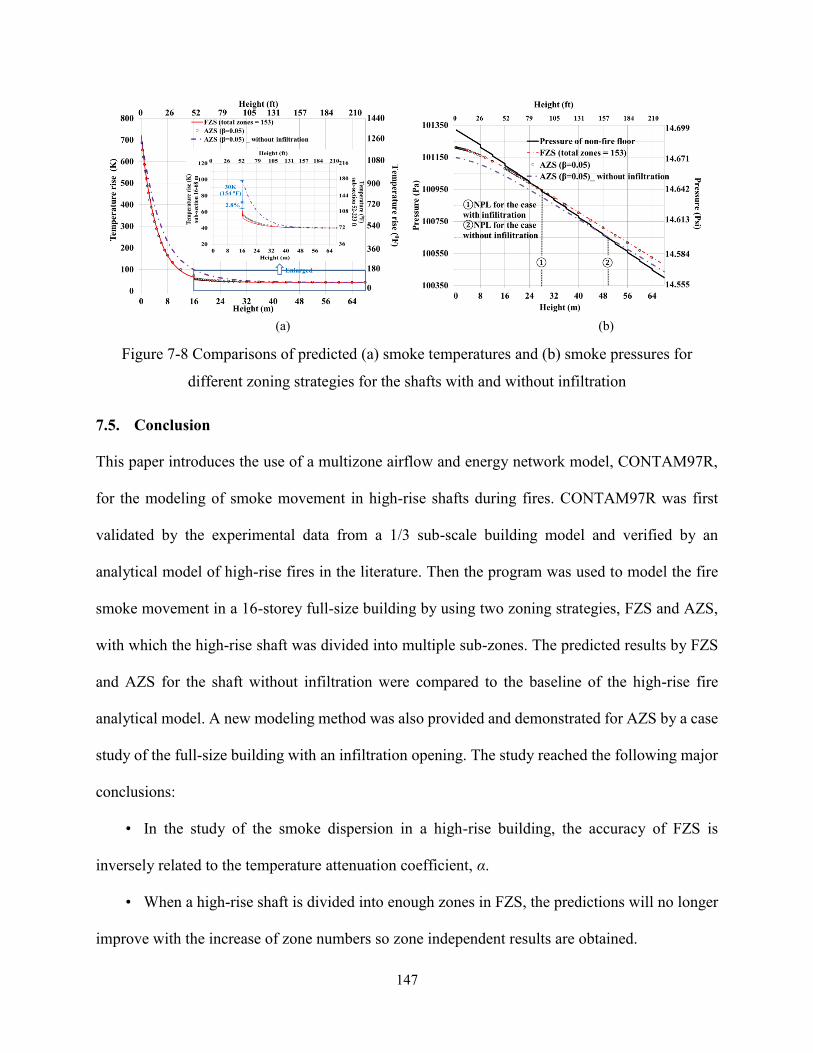
147

(a) (b)

Figure 7-8 Comparisons of predicted (a) smoke temperatures and (b) smoke pressures for

different zoning strategies for the shafts with and without infiltration

7.5. Conclusion

This paper introduces the use of a multizone airflow and energy network model, CONTAM97R,

for the modeling of smoke movement in high-rise shafts during fires. CONTAM97R was first

validated by the experimental data from a 1/3 sub-scale building model and verified by an

analytical model of high-rise fires in the literature. Then the program was used to model the fire

smoke movement in a 16-storey full-size building by using two zoning strategies, FZS and AZS,

with which the high-rise shaft was divided into multiple sub-zones. The predicted results by FZS

and AZS for the shaft without infiltration were compared to the baseline of the high-rise fire

analytical model. A new modeling method was also provided and demonstrated for AZS by a case

study of the full-size building with an infiltration opening. The study reached the following major

conclusions:

• In the study of the smoke dispersion in a high-rise building, the accuracy of FZS is

inversely related to the temperature attenuation coefficient, α.

• When a high-rise shaft is divided into enough zones in FZS, the predictions will no longer

improve with the increase of zone numbers so zone independent results are obtained.

148

• Compared to FZS, AZS provides results with similar accuracy as FZS but with fewer

zones.

• The case studies reveal that adding an infiltration opening lower than the NPL (e.g. pop up

a shaft door during a fire), may cause more smoke exposure at the non-fire floors above the fire

floor.

It should be noted that although this study is based on CONTAM97R, the proposed zoning

strategies and conclusions should also be applicable to other similar multi-zone airflow and energy

network models.

149

Chapter 8 Conclusion and Future Work

8.1. Conclusion

This research established an analytical model of couple heat and mass transfer of fire smoke spread

through non-adiabatic vertical shafts of high-rise shafts, which is comprised of energy balance

equation, mechanical energy equation, orifice equation and mass balance equation. On the basis

of the analytical model, simple calculation method and empirical equation of neutral plane level

were proposed. It was found that:

The temperature attenuation coefficient, α, a non-dimensional parameter associated with the

geometrical and thermal properties of the smoke and the shaft, is an important parameter for

the solutions of the coupled problem, because the temperature profiles of smoke and shaft wall

are both shown to be exponential functions of α.

The analytical solution provides the important information for the risk assessment of the smoke

spread from the fire floor to higher floors, including shaft top temperature, maximum mass

flow rate and corresponding fire floor temperature, and location of NPL.

For non-adiabatic shafts, the effects of non-uniform temperature distribution on NPL should

be considered. The provided case study shows that the uniform temperature assumption leads

to over-estimated NPL, and the relation between shaft bottom/top temperature and NPL

predicted based on this assumption is inconsistent to that of the experiments.

Non-uniform temperature distribution inside of the shaft can be represented by a dimensionless

number, TshH/Ta, which is a ratio of shaft top temperature to ambient temperature. This

dimensionless number is a function of temperature attenuation coefficient, α, which indicates

smoke temperature profile inside the shaft.

150

The sensitivity study found that the developed empirical equations, which include the

dimensionless number in terms of TshH and Tsh0, can predict NPL accurately. The existing

equation may either underestimate or overestimate the NPL locations.

Studies on the dimensionless analytical solutions and similarity were also conducted based on the

analytical model, which lead to a better understanding of the physics of smoke movement through

vertical shafts as well as developing a new scaling method to sub-scale smoke spreads in high-rise

shafts. Experiments on different size and material shafts were designed and carried out, the results

of which were used to verify the dimensionless analytical solutions and the new scaling method.

The study found that:

The developed dimensionless model could predict accurate temperature distribution, mass

flow rate and neutral plane level. The measured parameters of experiments are close to the

predicted results of the dimensionless model.

By defining the dimensionless number, ω, which equals to ψ times α, the coupled problem of

smoke movement inside shaft driven by stack effect can be solved by only two equations,

which much simplifies the calculations that cannot be achieved by previous studies.

For the natural venting, with the increase of fire strength, smoke flow rate through the shaft

increases accordingly whereas the temperature gradient does not change significantly, thus

leading to minor change of NPL.

The temperature attenuation coefficient, α, is in a form of the Stanton number, St, which is the

ratio of the heat loss of the smoke over the thermal capacity of the smoke. When the mechanical

venting rate (ψ) is increased in a shaft, St, becomes smaller, indicating less heat loss from

smoke or more smoke thermal capacity, and thus the vertical temperature gradient decreases.

151

The adiabatic assumption, which is commonly used in the literature, is found to lead to an

overestimation of the mechanical venting rate necessary to keep a high-rise shaft free of smoke.

The resultant error depends on the dimensionless number, ω, describing the geometry and

thermal properties of the shaft: the adiabatic assumption causes more errors for bigger values

of ω.

By using the discharge coefficient, Cd, to express the inside structure resistance of the shaft,

the shaft with inside structure, like shaft with stairs, could be sub-scaled as the shaft without

inside structure, which is simpler to model.

By considering heat transfer between smoke and the boundaries, and the interior structure

resistance, the new modeling method could achieve more accurate results than Froude

modeling method.

Based on the multizone program with an added energy equation, CONTAM97R, which has the

capability of calculating the coupled heat and mass transfer inside the high-rise shafts, a numerical

modeling method was developed. The numerical modeling method employs a new zoning strategy

called adaptive zoning strategy (AZS), which adapts the temperature gradient inside the shaft. The

following conclusions could be achieved:

In the study of the smoke dispersion in a high-rise building, the accuracy of FZS is inversely

related to the temperature attenuation coefficient, α.

When a high-rise shaft is divided into enough zones in FZS, the predictions will no longer

improve with the increase of zone numbers so zone independent results are obtained.

Compared to FZS, AZS provides results with similar accuracy as FZS but with fewer zones.

The case studies reveal that adding an infiltration opening lower than the NPL (e.g. popping

up a shaft door during a fire), may cause more smoke exposure at the non-fire floors above the

152

fire floor.

8.2. Future work

Analytical and similarity studies of smoke movement in high-rise shafts under transient state

condition

This thesis is focused on the steady state, the related parameters under which condition are

vital for understanding physics of fire smoke movement and the design of the fire smoke

protection system. The transient state is also important for the study of fire smoke protection,

because during the time of transient state, it is the very important for people to evacuate the

high-rise buildings. Therefore, it is also necessary to do the analytical and similarity studies of

smoke movement in high-rise shafts under transient state condition.

Determination of values of constants in the NPL empirical equations

Chapter 5 presents NPL empirical equations, which is helpful to understand the underlying

physics regarding the NPL in high-rise shafts. The constants C1, N1 and C2 of the empirical

equations needs to be correlated by more experiments on different size and material shafts, so

that the empirical equations could be used to design fire smoke protection shafts.

Similarity studies of smoke movement in the whole building

Sub-scaled experiments are important for the research of fire smoke movement in buildings.

High-rise shaft is the main space for toxic smoke spreading to higher levels rapidly due to stack

effect, and is the subject for the similarity study in this thesis. Previous study has reported the

scaling method in a single fire room. It would be meaningful to study the similarity law of

smoke movement in the whole building, where the smoke spreads from the fire room to the

higher level of the high-rise building through openings between shafts and non-fire floor

located at the higher level.

153

Integrate the analytical model into the control strategy of high-rise fire protection system

During the high-rise fires, it is pretty important to indicate where the smoke has spread to and

how much smoke flows inside the shafts. Therefore, prediction of neutral plane level and flow

rate of smoke for high-rise shafts are useful for the high-rise fire protection system. In this

thesis, the analytical model in terms of dimensionless numbers has been developed. Further

studies could focus on the integration of the analytical model into the control strategy of high-

rise fire protection system to predict and control neutral plane level and flow rate of smoke for

shafts.

154

Reference

Allison C. Carey. 2010. “Scale Modeling of Static Fires in a Complex Geometry for Forensic Fire

Applications.” Msc. thesis. University of Maryland, College Park.

ASHRAE. 2009. ASHRAE Handbook–fundamentals. Atlanta, GA: American Society of Heating,

Refrigerating and Air Conditioning Engineers.

ASTM D5157-97. 2008. Standard Guide for Statistical Evaluation of Indoor Air Quality Models.

West Conshohocken, PA.

Axley, J.W. 2011. Application of Natural Ventilation for U.S. Commercial Buildings: Climate

Suitability Design Strategies & Methods Modeling Studies. Reference Number: GCR-01-820.

Gaithersburg, MD. http://web.stanford.edu/group/narratives/classes/08-

09/CEE215/ReferenceLibrary/Natural Ventilation/Natural Ventilation in US Commercial

Buildings.pdf.

Axley, James W, Ph D, Steven J Emmerich, and George N Walton. 2002. “Modeling the

Performance of a Naturally Ventilated Commercial Building with a Multizone Coupled

Thermal / Airflow Simulation Tool.” ASHRAE Transactions 108 (2): 1260–1275.

Bae, Sungryong, Hyun-Jun Shin, and Hong-Sun Ryou. 2014. “Development of CAU_USCOP, a

Network-Based Unsteady Smoke Simulation Program for High-Rise Buildings.” Building

Simulation 7 (5): 503–510. doi:10.1007/s12273-014-0172-9.

Beitel, Jesse J., Alison J. Wakelin, and Craig L. Beyler. 2000. Analysis of Smoke Movement in a

Building via Elevator Shafts. Beaverton, OR.

Black, W. Z. 2009. “Smoke Movement in Elevator Shafts during a High-Rise Structural Fire.” Fire

Safety Journal 44 (2): 168–182. doi:10.1016/j.firesaf.2008.05.004.

Black, W. Z. 2010. “COSMO-Software for Designing Smoke Control Systems in High-Rise

155

Buildings.” Fire Safety Journal 45 (6-8). Elsevier: 337–348.

doi:10.1016/j.firesaf.2010.07.001.

CBC news. 2014. “130 Highrise Building Projects in Toronto Lead North America.” CBC.

http://www.cbc.ca/news/business/130-highrise-building-projects-in-toronto-lead-north-

america-1.2504776.

Chan, Y H. 2003. “Biostatistics 104: Correlational Analysis.” Singapore Medical Journal 44 (12):

614–619.

Chappell, Bill. 2016. “Fire At Dubai High-Rise Is Blamed On Electrical Issue In Spotlight.” NPR.

http://www.npr.org/sections/thetwo-way/2016/01/20/463691162/fire-at-dubai-high-rise-

tower-is-blamed-on-electrical-issue-in-spotlight.

Chen, Qingyan. 2009. “Ventilation Performance Prediction for Buildings: A Method Overview

and Recent Applications.” Building and Environment 44 (4). Elsevier Ltd: 848–858.

doi:10.1016/j.buildenv.2008.05.025.

Chow, W. K., and Henry H. W. Lo. 2008. “Scale Modeling on Natural Smoke Filling in an Atrium.”

Heat Transfer Engineering 29 (1): 76–84. doi:10.1080/09647040701677565.

Chow, W. K., and W.M. Siu. 1993. “Visualization of Smoke Movement in Scale Models of

Atriums.” JJournal of Applied Fire Science 3 (2): 93–111.

Chow, W. K., and J. H. Zhao. 2011. “Scale Modeling Studies on Stack Effect in Tall Vertical

Shafts.” Journal of Fire Sciences 29 (6): 531–542. doi:10.1177/0734904111410657.

Colaco, Joseph, Girish Dravid, and Vikas Kasilwal. 2012. “The Design and Construction of the

Palais Royale , Mumbai.” In CTBUH 2012 9th World Congress, edited by Council on Tall

Buildings and Urban Habitat, 686–692. Shanghai, China.

Ding, Wenting, Yoshikazu Minegishi, Yuji Hasemi, and Tokiyoshi Yamada. 2004. “Smoke

156

Control Based on a Solar-Assisted Natural Ventilation System.” Building and Environment

39 (7): 775–782. doi:10.1016/j.buildenv.2004.01.002.

Dols, W Stuart, and Brian J Polidoro. 2015. CONTAM User Guide and Program Documentation.

Gaithersburg, MD: National Institute of Standards and Technology.

“Dubai Hotel Fire Could Have Been Worse.” 2016. European Fire Sprinkler Network.

http://eurosprinkler.org/dubai-hotel-fire-could-have-been-worse/.

EN 12101-3 Standard. 2002. Smoke and Heat Control Systems-Part 3: Specification for Powered

Smoke and Heat Exhaust Ventilators. Brussels, Belgium.

Ferreira, M.J., and S.M. Strege. 2005. Smoke Management Systems: Federal Building and Fire

Safety Investigation of the World Trade Center Disaster, Report, NIST NCSTAR 1-4D.

Gaithersburg, MD. http://fire.nist.gov/bfrlpubs/build05/PDF/b05039.pdf.

Gann, Richard G, Vytenis Babrauskas, Richard D Peacock, and John R Hall Jr. 1994. “Fire

Conditions for Smoke Toxicity Measurement.” Fire and Materials 18 (3): 193–199.

Gu, L. 2011. “Advanced of EnergyPlus and Its Coupling with CHAMPS-Whole Building.” In

Proceedings of CHAMPS 2011: The 8th International Forum and Workshop on Combined

Heat, Air, Moisture and Pollutant Simulations. Nanjing, China.

Guo, Lixia, Lei Guo, Ling Zhong, and Yueming Zhu. 2011. “Thermal Conductivity and Heat

Transfer Coefficient of Concrete.” Journal of Wuhan University of Technology-Mater. Sci.

Ed. 26 (4): 791–796. doi:10.1007/s11595-011-0312-3.

Hadjisophocleous, George, and Q. Jia. 2009. “Comparison of FDS Prediction of Smoke Movement

in a 10-Storey Building with Experimental Data.” Fire Technology 45 (2): 163–177.

doi:10.1007/s10694-008-0075-3.

Hall, J.R. 2011. High-Rise Building Fire. Quincy, MA.

157

Hall, John R. 2011. Fatal Effects of Fire. NFPA. Quincy, MA.

Harmathy, T. Z. 1998. “Simplified Model of Smoke Dispersion in Buildings by Stack Effect.” Fire

Tech 34 (1): 6–17. doi:10.1023/A:1015352714123.

Harmathy, T. Z., and I. Oleszkiewicz. 1987. “Fire Drainage System.” Fire Technology 23 (1): 26–

48. doi:10.1007/BF01038364.

Harrison, Roger. 2004. “Smoke Control in Atrium Buildings: A Study of the Thermal Spill Plume.”

M.S. thesis. University of Canterbury.

Hensen, J. 1999. “A Comparison of Coupled and Decoupled Solutions for Temperature and Air

Flow in a Building.” ASHRAE Transactions 105 (2): 962–969.

Hou, Long Fei, Ming Li, Wu Yuan Cui, and Yu Chen Liu. 2011. “Numerical Simulation and

Analysis of on-Building High-Rise Building Fires.” Procedia Engineering 11: 127–134.

doi:10.1016/j.proeng.2011.04.637.

Hutcheon, N.B., and G.O.P. Handegord. 1983. Building Science for a Cold Climate. Halethorpe,

MD: Construction Technology Centre Atlantic, Incorporated.

International Code Council. 2007. Building Code of New York State. New York State:

International Code Council, Inc.

ISO 834. 1975. Fire Resistance Tests. Geneva: Elements of Building Construction. International

Organisation for Standardisation.

Ji, J., L. J. Li, W. X. Shi, C. G. Fan, and J. H. Sun. 2013. “Experimental Investigation on the Rising

Characteristics of the Fire-Induced Buoyant Plume in Stairwells.” International Journal of

Heat and Mass Transfer 64: 193–201. doi:10.1016/j.ijheatmasstransfer.2013.04.030.

Ji, J., M. Li, Z.H. Gao, Y.F. Li, W.X. Shi, and J.H. Sun. 2016. “Experimental Investigation of

Combustion Characteristics under Different Ventilation Conditions in a Compartment

158

Connected to a Stairwell.” Applied Thermal Engineering, 1–12.

doi:10.1016/j.applthermaleng.2016.01.117.

Ji, Jie, Man Li, Yifan Li, Jiping Zhu, and Jinhua Sun. 2015. “Transport Characteristics of Thermal

Plume Driven by Turbulent Mixing in Stairwell.” International Journal of Thermal Sciences

89. Elsevier Masson SAS: 264–271. doi:10.1016/j.ijthermalsci.2014.11.009.

Jo, Jae Hun, Jae Han Lim, Seung Yeong Song, Myoung Souk Yeo, and Kwang Woo Kim. 2007.

“Characteristics of Pressure Distribution and Solution to the Problems Caused by Stack Effect

in High-Rise Residential Buildings.” Building and Environment 42 (1): 263–277.

doi:10.1016/j.buildenv.2005.07.002.

Karlasson, Bjorn, and James G Quintiere. 2002. Enclosure Fire Dynamics. New York, WA: CRC

Press.

Klote, John H. 2011. “Stairwell Smoke Control by Ventilation.” ASHRAE Transactions 117 (1):

478–486.

Klote, John H. 1991. A General Routine of Analyzing of Stack Effect. Report, NISTIR 4588.

National Institute of Standards and Technology. Gaithersburg, MD.

Klote, John H. 2004. “Analysis of the Life Safety Consequences of Smoke Migration Through

Elevator Shafts.” Elevator World 52 (11): 81–90.

Klote, John H., James A. Milke, Paul G. Turnbull, Ahmed Kashef, and Michael J. Ferreira. 2012.

Handbook of Smoke Control Engineering. Atlanta, GA.: American Society of Heating

Refrigerating and Air-Conditioning Engineers.

Lay, Simon. 2014. “Pressurization Systems Do Not Work & Present a Risk to Life Safety.” Case

Studies in Fire Safety 1 (1). Elsevier Ltd: 13–17. doi:10.1016/j.csfs.2013.12.001.

Li, L. J., J. Ji, C. G. Fan, J. H. Sun, X. Y. Yuan, and W. X. Shi. 2014. “Experimental Investigation

159

on the Characteristics of Buoyant Plume Movement in a Stairwell with Multiple Openings.”

Energy and Buildings 68 (Part A): 108–120. doi:10.1016/j.enbuild.2013.09.028.

Lie, T. T., and J. H. McGuire. 1975. “Control of Smoke in High-Rise Buildings.” Fire Technology

11 (1): 5–14. doi:10.1007/BF02589996.

Luo, Na, Angui Li, Ran Gao, Zhenguo Tian, Wei Zhang, Sen Mei, Luman Feng, and Pengfei Ma.

2013. “An Experiment and Simulation of Smoke Confinement and Exhaust Efficiency

Utilizing a Modified Opposite Double-Jet Air Curtain.” Safety Science 55: 17–25.

doi:10.1016/j.ssci.2012.12.002.

Marshall, N.R. 1986. “Air Entrainment into Smoke and Hot Gases in Open Shafts.” Fire Safety

Journal 10 (1): 37–46. doi:10.1016/0379-7112(86)90030-5.

McCaffrey, B. J., J. G. Quintiere, and M. F. Harkleroad. 1981. “Estimating Room Temperatures

and the Likelihood of Flashover Using Fire Test Data Correlations.” Fire Technology 17 (2):

98–119. doi:10.1007/BF02479583.

McDowell, T.P., S. Emmerich, J.W. Thornton, and G. Walton. 2003. “Integration of Airflow and

Energy Simulation Using CONTAM and TRNSYS.” ASHRAE Transactions 109 (1): 757–

770.

McGrattan, K., R. McDermott, C. Weinschenk, and K. Overholt. 2013. Fire Dynamics Simulator

User’s Guide. Gaithersburg, MD.

Mercier, G. P., and Y. Jaluria. 1999. “Fire-Induced Flow of Smoke and Hot Gases in Open Vertical

Enclosures.” Experimental Thermal and Fluid Science 19 (2): 77–84. doi:10.1016/S0894-

1777(99)00012-6.

Miller, Richard S, and Don Beasley. 2009. “On Stairwell and Elevator Shaft Pressurization for

Smoke Control in Tall Buildings.” Building and Environment 44 (6). Elsevier Ltd: 1306–

160

1317. doi:http://dx.doi.org/10.1016/j.buildenv.2008.09.015.

Miller, Richard S. 2011. “Elevator Shaft Pressurization for Smoke Control in Tall Buildings: The

Seattle Approach.” Building and Environment 46 (11). Elsevier Ltd: 2247–2254.

doi:10.1016/j.buildenv.2011.05.007.

Munson, Bruce R., Donald F. Young, Theodore H. Okiishi, and Wade W. Huebsch. 2009.

Fundamentals of Fluid Mechanics. Sixth edit.

Musser, A., K. McGrattan, and J. Palmer. 2001. Evaluation of a Fast, Simplified Computation

Fluid Dynamics Model for Solving Room Airflow Problems. Report, NISTIR 6760.

Gaithersburg, MD.

NFPA 101. 2012. Life Safety Code, 2012 Ed. Quincy, MA.

Ng, L, a Musser, Ak Persily, and Sj Emmerich. 2012. “Airflow and Indoor Air Quality Models of

DOE Reference Commercial Buildings.” Gaithersburg, MD, National ….

http://www.bfrl.nist.gov/IAQanalysis/docs/Tech Note 1734 - CONTAM reference bldgs.pdf.

Ng, Lisa C., Amy Musser, Andrew K. Persily, and Steven J. Emmerich. 2013. “Multizone Airflow

Models for Calculating Infiltration Rates in Commercial Reference Buildings.” Energy and

Buildings 58: 11–18. doi:10.1016/j.enbuild.2012.11.035.

Peppes, a a, M Santamouris, and D N Asimakopoulos. 2001. “Buoyancy-Driven Flow through a

Stairwell.” Building and Environment 36 (2): 167–180.

Peppes, a a, M Santamouris, and D N Asimakopoulos. 2002. “Experimental and Numerical Study

of Buoyancy-Driven Stairwell Ow in a Three Storey Building.” Building and Environment

37 (5): 497–506.

Poreh, M, and S Trebukov. 2000. “Wind Effects on Smoke Motion in Buildings” 35 (3): 257–273.

Qi, Dahai, Liangzhu Wang, and Radu Zmeureanu. 2014a. “An Analytical Model of Heat and Mass

161

Transfer through Non-Adiabatic High-Rise Shafts during Fires.” International Journal of

Heat and Mass Transfer 72. Elsevier Ltd: 585–594.

doi:10.1016/j.ijheatmasstransfer.2014.01.042.

Qi, Dahai, Liangzhu Wang, and Radu Zmeureanu. 2014b. “A Hand Calculation Method of Smoke

Movement through High-Rise Building Shaft.” In ASHRAE Annual Conference 2014.

Seattle, WA.

Qi, Dahai, Liangzhu Wang, and Radu Zmeureanu. 2015. “Modeling Smoke Movement in Shafts

during High-Rise Fires by a Multizone Airflow and Energy Network Program.” ASHRAE

Transactions 121 (2).

Qi, Dahai, Liangzhu Wang, and Radu Zmeureanu. 2016. “The Effects of Non-Uniform

Temperature Distribution on Neutral Plane Level in Non-Adiabatic High-Rise Shafts During

Fires.” Fire Technology. Springer US. doi:10.1007/s10694-015-0554-2.

Quintiere, James G, and Michael E Dillon. 2008. “Scale Model Reconstruction of Fire in an

Atrium.” In Progress in Scale Modeling, 109–120.

Sahlin, P. 2003. “On the Effects of Decoupling Airflow and Heat Balance in Building Simulation

Models.” ASHRAE Transactions 109 (2): 1671–1677.

Shi, W. X., J. Ji, J. H. Sun, S. M. Lo, L. J. Li, and X. Y. Yuan. 2014a. “Influence of Staircase

Ventilation State on the Airflow and Heat Transfer of the Heated Room on the Middle Floor

of High Rise Building.” Applied Energy 119: 173–180. doi:10.1016/j.apenergy.2013.12.055.

Shi, W. X., J. Ji, J. H. Sun, S. M. Lo, L. J. Li, and X. Y. Yuan. 2014b. “Influence of Fire Power

and Window Position on Smoke Movement Mechanisms and Temperature Distribution in an

Emergency Staircase.” Energy and Buildings 79: 132–142.

doi:10.1016/j.enbuild.2014.02.083.

162

Siegel, R., and J.R. Howell. 1993. Thermal Radiation Heat Transfer. third ed. Washington, DC:

Hemisphere Publishing Corporation.

Steckler, K D, H R Baum, and A X J G Quintiere. 1986. “Multicompartment Enclosures Elements

of Salt Water Modeling.” Twenty-First Symposium (International)on Combustion/The

Combustion Institute, 143–149.

Su, Chung Hwei, Yu Chang Lin, Chi Min Shu, and Ming Chih Hsu. 2011. “Stack Effect of Smoke

for an Old-Style Apartment in Taiwan.” Building and Environment 46 (12): 2425–2433.

doi:10.1016/j.buildenv.2011.04.026.

Sun, X. Q., L. H. Hu, W. K. Chow, Y. Xu, and F. Li. 2011. “A Theoretical Model to Predict Plume

Rise in Shaft Generated by Growing Compartment Fire.” International Journal of Heat and

Mass Transfer 54 (4): 910–920. doi:10.1016/j.ijheatmasstransfer.2010.10.012.

Tamura, G.T. 1994. Smoke Movement & Control in High-Rise Buildings. Quincy, MA.: National

Fire Protection Association.

Tang, G. 2005. “Study of Natural Ventilation Design by Integrating the Multizone Model with

CFD Simulation.” Ph.D. thesis. Massachusetts Institute of Technology,Cambridge, MA.

Tang, G., and Leon R. Glicksman. 2005. “Application of Integrating Multi-Zone Model with CFD

Simulation to Natural Ventilation Prediction.” Energy and Buildings 37 (10): 1049–1057.

doi:10.1016/j.enbuild.2004.12.009.

Walton, George N, and W Stuart Dols. 2013. CONTAM User Guide and Program Documentation.

Gaithersburg, MD.: National Institute of Standards and Technology.

Wang, Liangzhu, William Z Black, and Guanchao Zhao. 2013. “Comparison of Simulation

Programs for Airflow and Smoke Movement during High-Rise Fires.” ASHRAE

Transactions 119 (2): 12.

163

Wang, Liangzhu, and Qingyan Chen. 2008. “Evaluation of Some Assumptions Used in Multizone

Airflow Network Models.” Building and Environment 43 (10): 1671–1677.

doi:10.1016/j.buildenv.2007.10.010.

Wang, Liangzhu Leon, W Stuart Dols, and Steven J Emmerich. 2012. “Simultaneous Solutions of

Coupled Thermal Airflow Problem for Natural Ventilation in Buildings Simultaneous

Solutions of Coupled Thermal Airflow Problem for Natural Ventilation in Buildings,” no.

April 2013: 37–41. doi:10.1080/10789669.2011.591258.

Wang, Yan, Ehab Zalok, and George Hadjisophocleous. 2011. “An Experimental Study of Smoke

Movement in Multi-Storey Buildings.” Fire Technology 47 (4): 1141–1169.

doi:10.1007/s10694-009-0132-6.

Wood, Antony, and Salib， Ruba. 2013. Natural Ventilation in High-Rise Office Buildings.

Routledge. Chicago, IL: Routledge.

https://store.ctbuh.org/PDF_Previews/Reports/2012_CTBUHNaturalVentilationGuide_Prev

iew.pdf.

Xiao, G. Q., J. Y. Tu, and G. H. Yeoh. 2008. “Numerical Simulation of the Migration of Hot Gases

in Open Vertical Shaft.” Applied Thermal Engineering 28 (5-6): 478–487.

doi:10.1016/j.applthermaleng.2007.05.006.

Yam, Jimmu, Yuguo Li, and Zuohuan Zheng. 2008. “Coupling of Thermal Mass and Natural

Ventilation in Buildings.” Energy and Buildings 40 (6): 979–986.

doi:10.1016/j.enbuild.2007.08.001.

Yang, Dong, Tao Du, Shini Peng, and Baizhan Li. 2013. “A Model for Analysis of Convection

Induced by Stack Effect in a Shaft with Warm Airflow Expelled from Adjacent Space.”

Energy and Buildings 62: 107–115. doi:10.1016/j.enbuild.2013.02.045.

164

Yang, Dong, Bai Zhan Li, Tao Du, and Nan Li. 2012. “Analytical Models for Evaluating

Buoyancy-Driven Ventilation due to Stack Effect in a Shaft Considering Heat Transfer from

Shaft Interior Boundaries.” Journal of Central South University of Technology (English

Edition) 19 (3): 651–656. doi:10.1007/s11771-012-1052-z.

Yii, Ee Hieng. 1998. Exploratory Salt Water Experiments of Balcony Spill Plume Using Laser

Induced Flurescent Technique. Fire Engineering Research Report 98/7. Christchurch.

file:///C:/Users/dahai/Downloads/FireEngResearchReport98-7.pdf.

Zhai, Zhiqiang, Mary Hall Johnson, and Moncef Krarti. 2011. “Assessment of Natural and Hybrid

Ventilation Models in Whole-Building Energy Simulations.” Energy and Buildings 43 (9).

Elsevier B.V.: 2251–2261. doi:10.1016/j.enbuild.2011.06.026.

Zhang, J. Y., W. Z. Lu, R. Huo, and R. Feng. 2008. “A New Model for Determining Neutral-Plane

Position in Shaft Space of a Building under Fire Situation.” Building and Environment 43 (6):

1101–1108. doi:10.1016/j.buildenv.2007.02.004.

Zhao, G., and L. Wang. 2014. “Using Helium Smoke as a Surrogate of Fire Smoke for the Study

of Atrium Smoke Filling.” Journal of Fire Sciences 32 (5): 431–447.

doi:10.1177/0734904114529403.

Zhong, Maohua, Weicheng Fan, T. M. Liu, P. H. Zhang, X. Wei, and G. X. Liao. 2004. “China:

Some Key Technologies and the Future Developments of Fire Safety Science.” Safety

Science 42 (7): 627–637. doi:10.1016/j.ssci.2003.10.003.