Analytical and Computer Cartography Winter 2017

Lecture 7: Spatial Data Structures for

Mapping

What is a Map Data Structure?

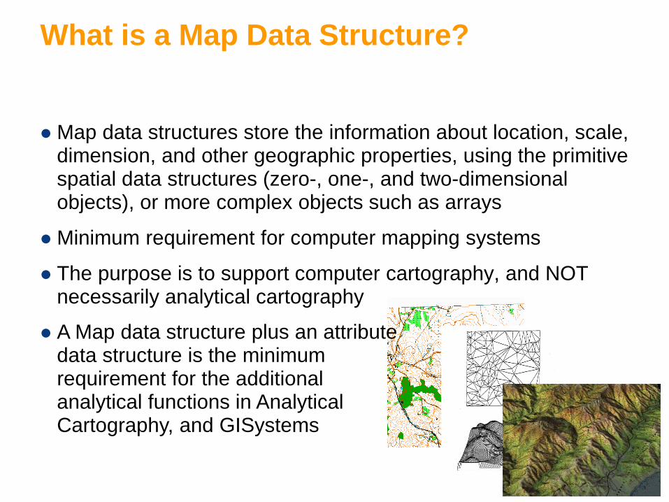
Map data structures store the information about location, scale, dimension, and other geographic properties, using the primitive spatial data structures (zero-, one-, and two-dimensional objects), or more complex objects such as arrays

Minimum requirement for computer mapping systems

The purpose is to support computer cartography, and NOT necessarily analytical cartography

A Map data structure plus an attribute data structure is the minimum requirement for the additional analytical functions in Analytical Cartography, and GISystems

Map Data Structures are largely Input-Determined

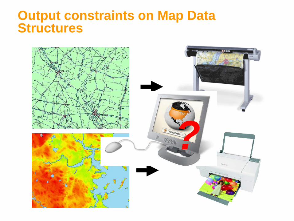
Output constraints on Map Data Structures

?

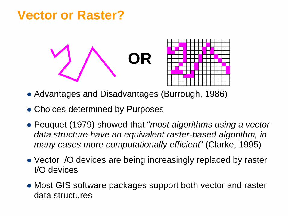
Vector or Raster?

Advantages and Disadvantages (Burrough, 1986)

Choices determined by Purposes

Peuquet (1979) showed that “most algorithms using a vector data structure have an equivalent raster-based algorithm, in many cases more computationally efficient” (Clarke, 1995)

Vector I/O devices are being increasingly replaced by raster I/O devices

Most GIS software packages support both vector and raster data structures

OR

Vectors just seemed more correcter

Can represent point, line, and area features very accurately

Far more efficient than raster data in terms of storage

Preferred when topology is concerned

Support interactive retrieval, which enables map generalization

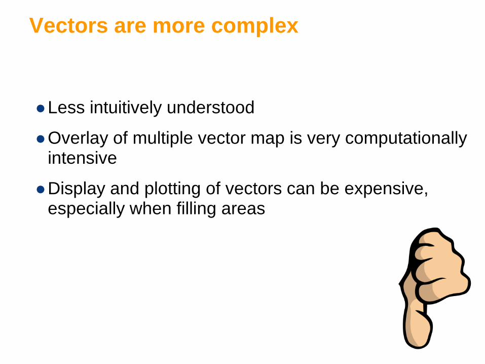
Vectors are more complex

Less intuitively understood

Overlay of multiple vector map is very computationally intensive

Display and plotting of vectors can be expensive, especially when filling areas

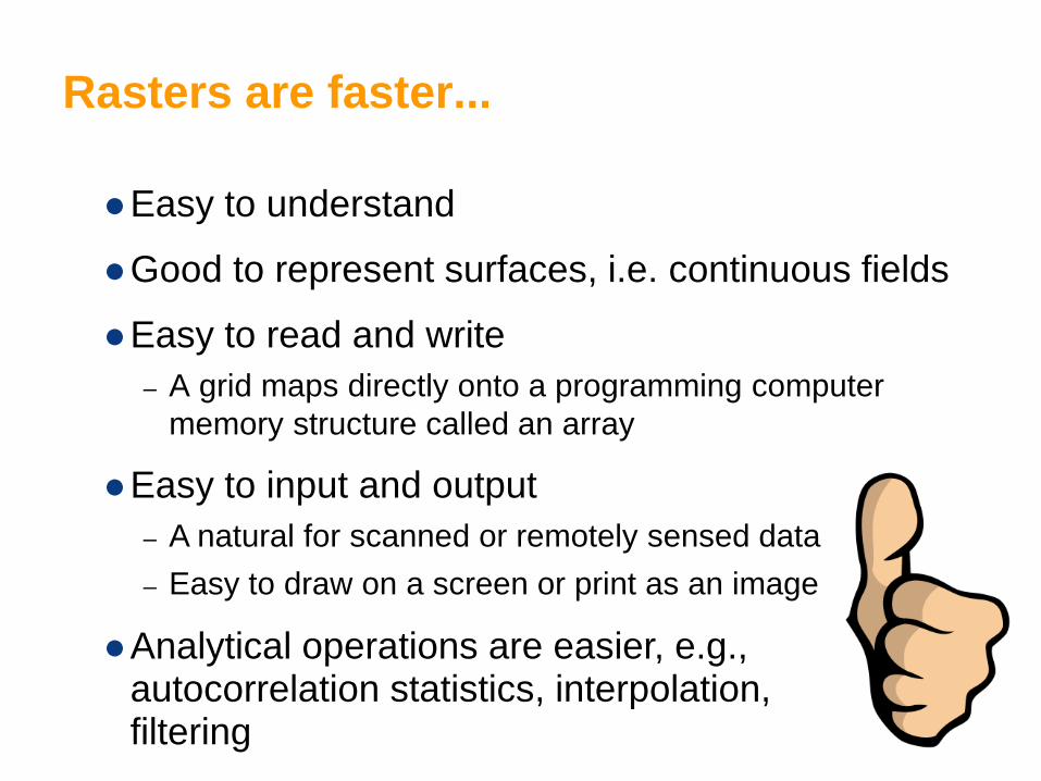
Rasters are faster...

Easy to understand

Good to represent surfaces, i.e. continuous fields

Easy to read and write – A grid maps directly onto a programming computer

memory structure called an array

Easy to input and output – A natural for scanned or remotely sensed data – Easy to draw on a screen or print as an image

Analytical operations are easier, e.g., autocorrelation statistics, interpolation, filtering

Rasters are bigger

Inefficient for storage – Raster compression techniques might not be efficient when dealing with

extremely variable data – Using large cells to reduce data volume causes information loss

Poor at representing points, lines and areas – Points and lines in raster format have to move to a cell center – Lines can become fat

Areas may need separately coded edges Each cell can be owned by only one feature

Good only at very localized topology, and weak otherwise

Suffer from the mixed pixel problem

Must often include redundant or missing data

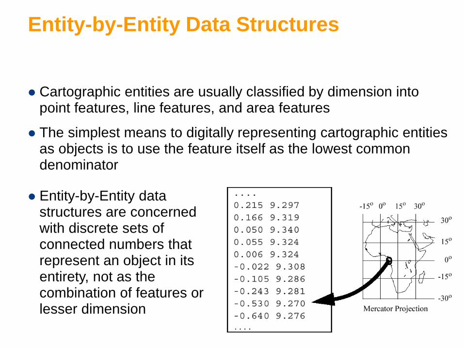
Entity-by-Entity Data Structures

Cartographic entities are usually classified by dimension into point features, line features, and area features

The simplest means to digitally representing cartographic entities as objects is to use the feature itself as the lowest common denominator

Entity-by-Entity data structures are concerned with discrete sets of connected numbers that represent an object in its entirety, not as the combination of features or lesser dimension

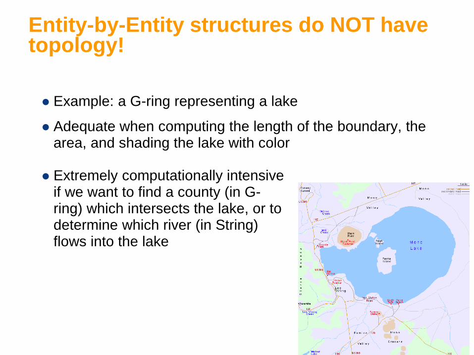
Entity-by-Entity structures do NOT have topology!

Example: a G-ring representing a lake

Adequate when computing the length of the boundary, the area, and shading the lake with color

Extremely computationally intensive

if we want to find a county (in G-ring) which intersects the lake, or to determine which river (in String) flows into the lake

Entity-by-Entity Data Structures - Point Objects (Vector)

Point list – (X, Y) coordinates – Feature codes – the keys linked to the attribute database

Point File Attribute Database

Keys

Entity-by-Entity Data Structures - Point Objects (Raster)

Point Index values (or attributes) assigned to cells; indices as the keys to the attribute database

One-pixel size

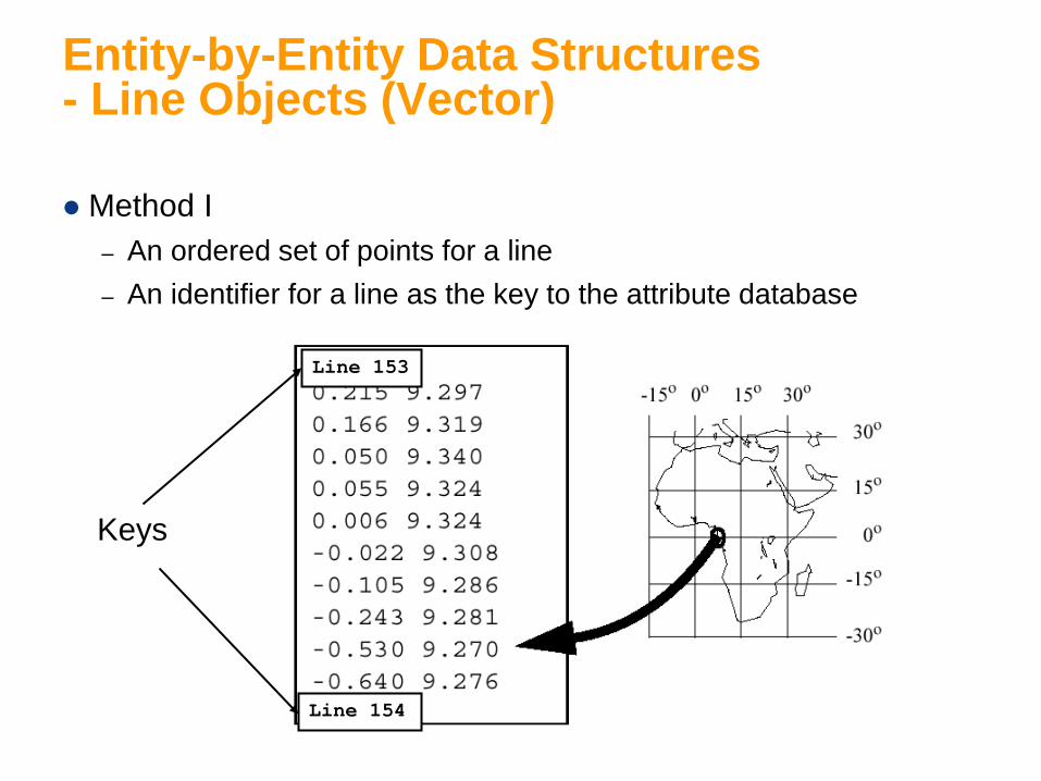
Entity-by-Entity Data Structures - Line Objects (Vector)

Method I – An ordered set of points for a line – An identifier for a line as the key to the attribute database

Line 153

Line 154

Keys

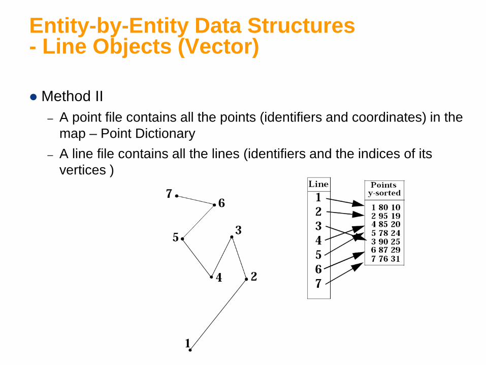
Entity-by-Entity Data Structures - Line Objects (Vector)

Method II – A point file contains all the points (identifiers and coordinates) in the

map – Point Dictionary – A line file contains all the lines (identifiers and the indices of its

vertices )

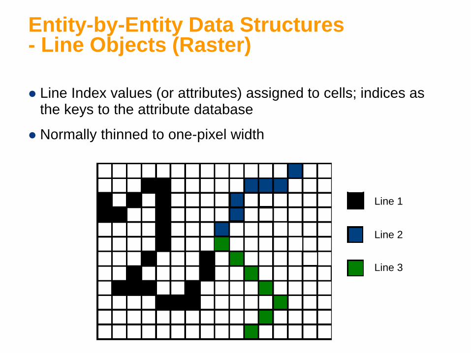
Entity-by-Entity Data Structures - Line Objects (Raster)

Line Index values (or attributes) assigned to cells; indices as the keys to the attribute database

Normally thinned to one-pixel width

Line 1

Line 2

Line 3

Vector Freeman codes

Raster Freeman codes – Length = 1 in primary directions – Length = in diagonal directions

Run-length for Freeman codes

Entity-by-Entity Data Structures - Line Objects (Freeman codes)

Freeman codes - a line as a sequence of octal (8-based) digits, each digit represents the direction of a step moved along the line

2

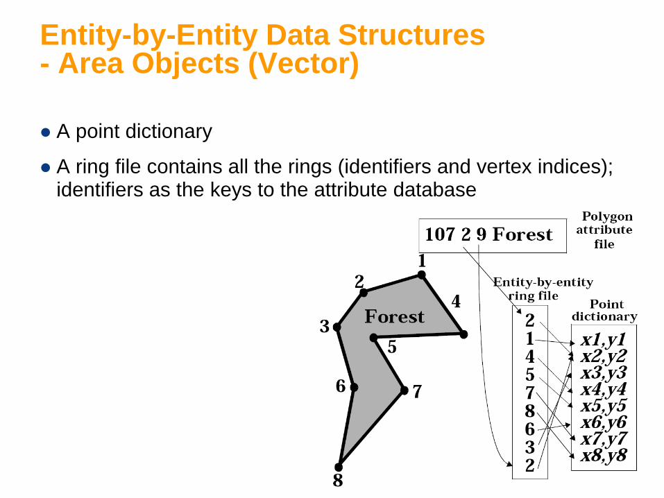
Entity-by-Entity Data Structures - Area Objects (Vector)

A point dictionary

A ring file contains all the rings (identifiers and vertex indices); identifiers as the keys to the attribute database

Entity-by-Entity Data Structures - Area Objects (Raster)

Polygon Index values (or attributes) assigned to cells; indices as keys to the attribute database

Area calculation by counting cells Run-length encoding could be efficient if the data is spatially

homogeneous

Topological Data Structures

Store the additional characteristics of connectivity and adjacency

Linkage between Primitive Objects (nodes, links, chains)

Forward linkage and Reverse linkage

Finite number of chains can meet at a node

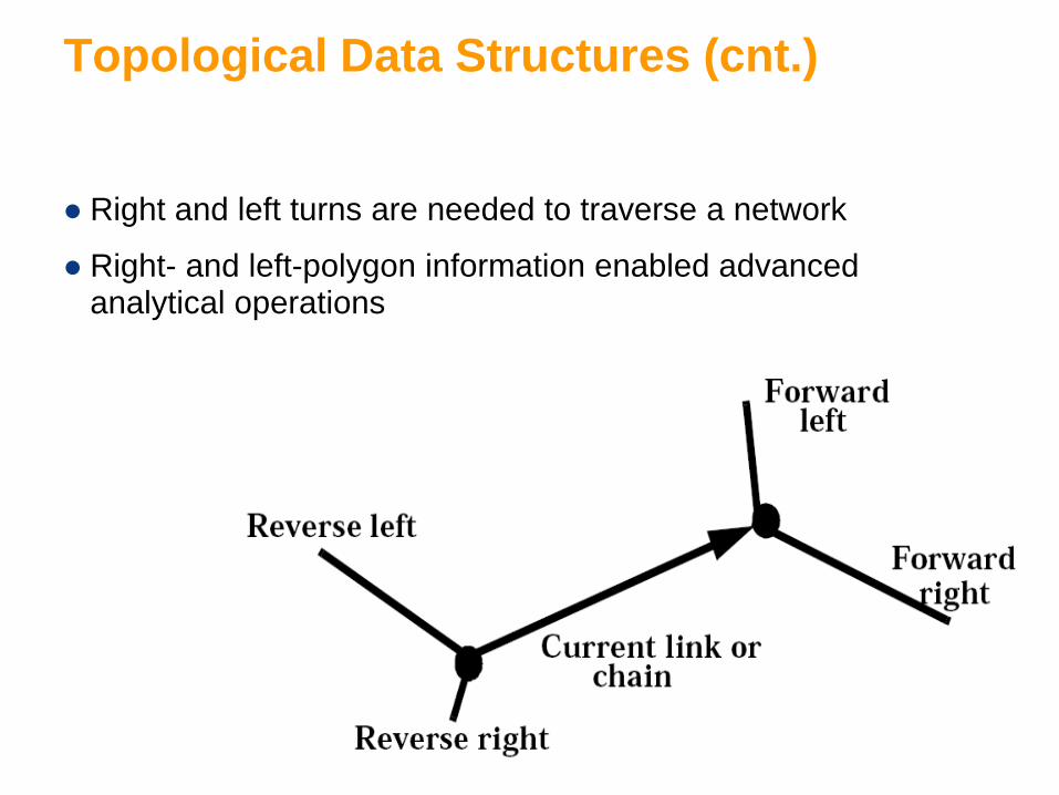
Topological Data Structures (cnt.)

Right and left turns are needed to traverse a network

Right- and left-polygon information enabled advanced analytical operations

Tessellations and the TIN

Tessellations are connected networks that partition space into a set of sub-areas

Regions of geographic interest – Political regions – states, countries – Grids

Triangulated Irregular Networks (TIN)

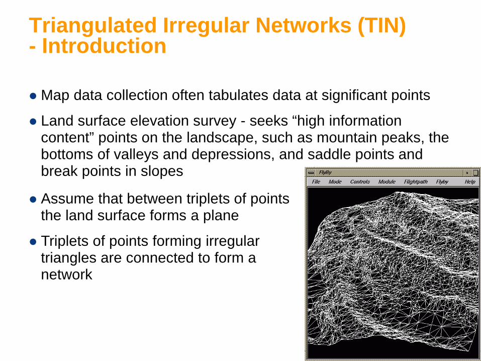
Triangulated Irregular Networks (TIN) - Introduction

Map data collection often tabulates data at significant points

Land surface elevation survey - seeks “high information content” points on the landscape, such as mountain peaks, the bottoms of valleys and depressions, and saddle points and break points in slopes

Assume that between triplets of points the land surface forms a plane

Triplets of points forming irregular triangles are connected to form a network

Triangulated Irregular Networks (TIN) - Creation

Delaunay triangulation to create TIN – Iterative process – Begins by searching for the closest two nodes – Then assigns additional nodes to the network if the triangles they

create satisfy a criterion, e.g. selecting the next triangle that is closest to a regular equilateral triangle

Outer edge is convex hull

Triangulated Irregular Networks (TIN) - Advantages

More accurate and use less space than grids

Can be generated from point data faster than grids.

Can describe more complex surfaces than grids, including vertical drops and irregular boundaries

Single points can be easily added, deleted, or moved

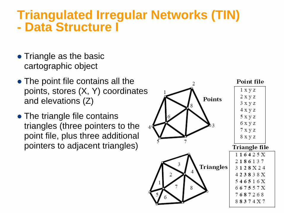
Triangulated Irregular Networks (TIN) - Data Structure I

Triangle as the basic cartographic object

The point file contains all the points, stores (X, Y) coordinates and elevations (Z)

The triangle file contains triangles (three pointers to the point file, plus three additional pointers to adjacent triangles)

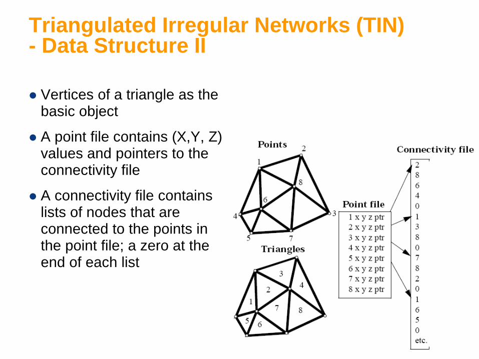
Triangulated Irregular Networks (TIN) - Data Structure II

Vertices of a triangle as the basic object

A point file contains (X,Y, Z) values and pointers to the connectivity file

A connectivity file contains lists of nodes that are connected to the points in the point file; a zero at the end of each list

Quad-tree Data Structures

A type of tessellation data structures Partition the space into nested squares -quadrants Index methods

– NE, SW, NE, NW, SE – Morton number

Allow very rapid area searches and relatively fast display

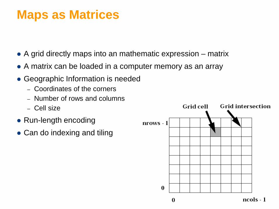
Maps as Matrices

A grid directly maps into an mathematic expression – matrix A matrix can be loaded in a computer memory as an array Geographic Information is needed

– Coordinates of the corners – Number of rows and columns – Cell size

Run-length encoding Can do indexing and tiling

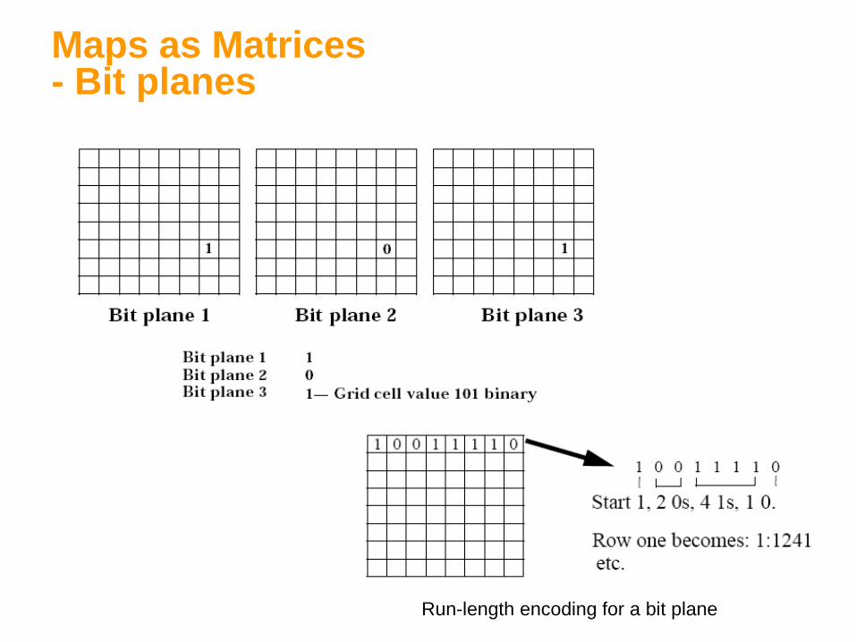
Maps as Matrices - Bit planes

Run-length encoding for a bit plane

Ad Hoc versus Standard Data Structures

Each GIS/mapping program uses its own standards

Wants rapid input/output and transformations

Wants to avoid computational errors and special cases

If structures are standards, programs can be reused and made as interchangeable parts

I/O routines can be written once and shared as libraries

E.g. ShapeLib: Routines to read and write ESRI .shp files and .dbf atttributes

Can also map directly onto display routines

Spatial Data Transfer Standard (SDTS) SDTS is “a robust way of transferring earth-referenced

spatial data between dissimilar computer systems with the potential for no information loss. It is a transfer standard that embraces the philosophy of self-contained transfers, i.e. spatial data, attribute, geo-referencing, data quality report, data dictionary, and other supporting metadata all included in the transfer” (USGS, http://mcmcweb.er.usgs.gov/sdts/)

Draft standard published in The American Cartographer (1988)

FIPS (Federal Information Processing Standards) 173 approved 1992

Standard consists of several parts

Open Geospatial Consortium

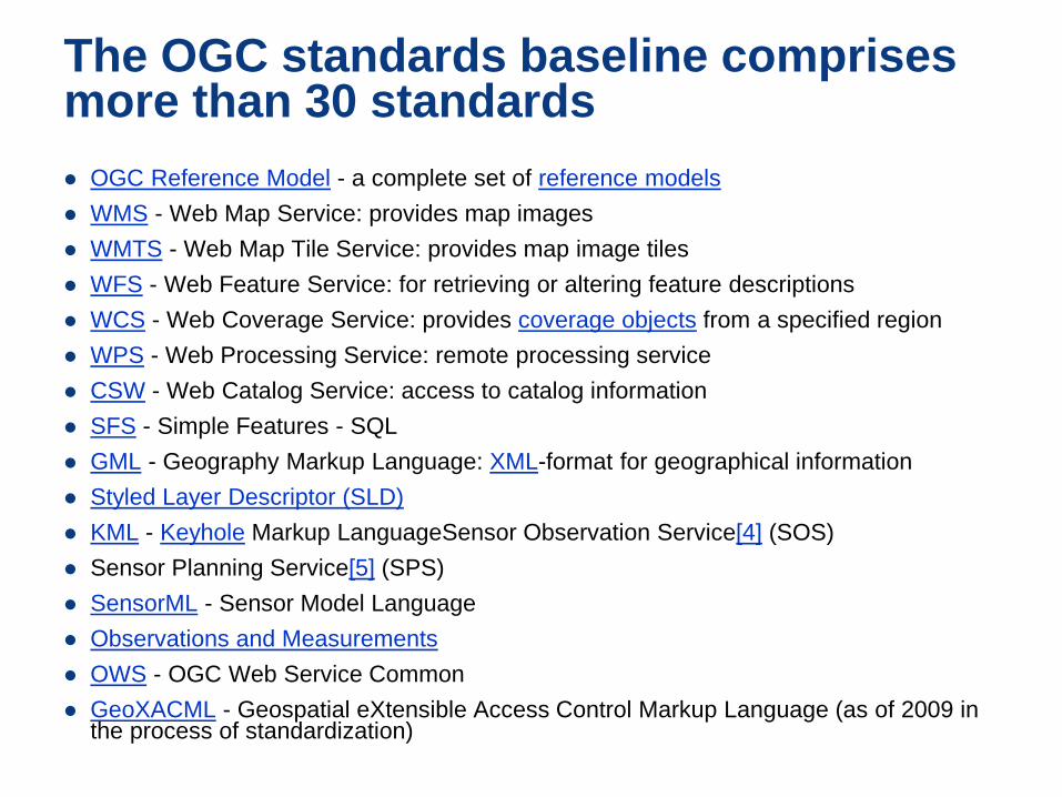
The OGC standards baseline comprises more than 30 standards OGC Reference Model - a complete set of reference models WMS - Web Map Service: provides map images WMTS - Web Map Tile Service: provides map image tiles WFS - Web Feature Service: for retrieving or altering feature descriptions WCS - Web Coverage Service: provides coverage objects from a specified region WPS - Web Processing Service: remote processing service CSW - Web Catalog Service: access to catalog information SFS - Simple Features - SQL GML - Geography Markup Language: XML-format for geographical information Styled Layer Descriptor (SLD) KML - Keyhole Markup LanguageSensor Observation Service[4] (SOS) Sensor Planning Service[5] (SPS) SensorML - Sensor Model Language Observations and Measurements OWS - OGC Web Service Common GeoXACML - Geospatial eXtensible Access Control Markup Language (as of 2009 in

the process of standardization)

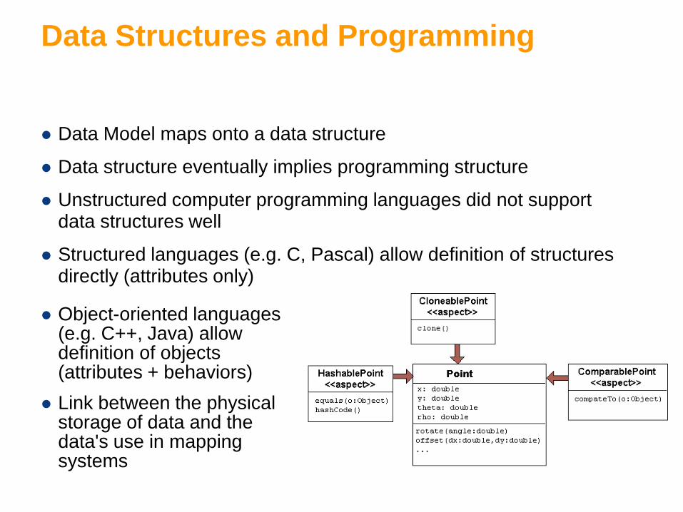
Data Structures and Programming

Data Model maps onto a data structure

Data structure eventually implies programming structure

Unstructured computer programming languages did not support data structures well

Structured languages (e.g. C, Pascal) allow definition of structures directly (attributes only)

Object-oriented languages (e.g. C++, Java) allow definition of objects (attributes + behaviors)

Link between the physical storage of data and the data's use in mapping systems

For example

C programming language

# Declare a grid – Int Grid[100][100]; – Grid[50][50] = 235;

# declare a Point Type – Typedef struct POINT { int point_id, double x, y;} – POINT Point[100]; – Point[50].x = 123231.0;

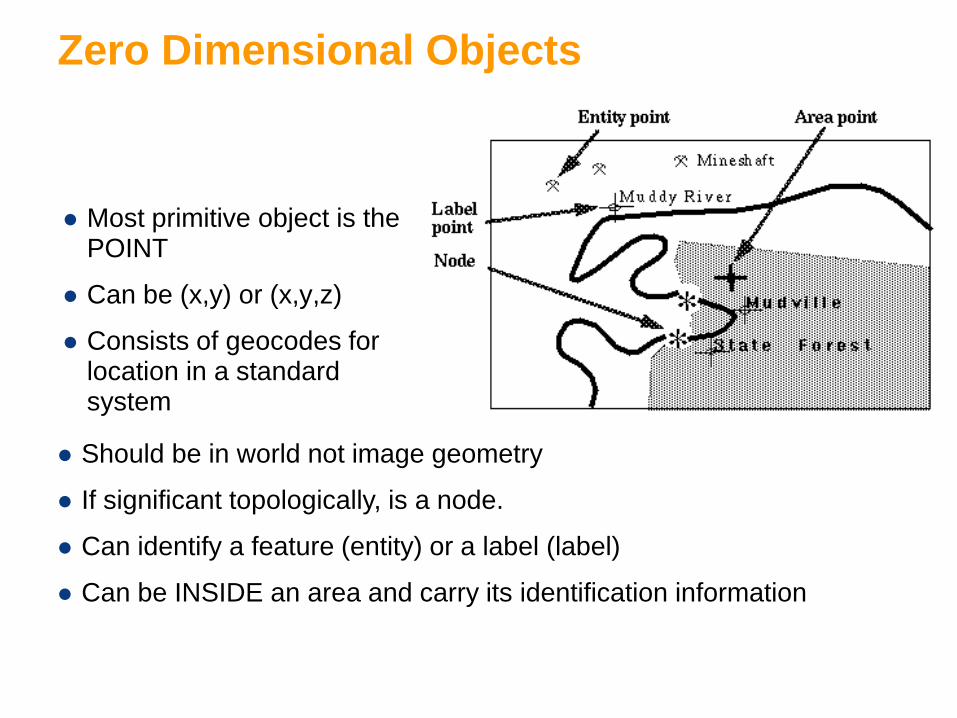
Zero Dimensional Objects

Most primitive object is the POINT

Can be (x,y) or (x,y,z)

Consists of geocodes for location in a standard system

Should be in world not image geometry

If significant topologically, is a node.

Can identify a feature (entity) or a label (label)

Can be INSIDE an area and carry its identification information

One Dimensional Objects

Divide up by lines with and without topological significance

Primitive object is the segment

Segments connect to make a string (line or polyline)

If defined mathematically, use arc

If line segment connects nodes, called a link (for a network)

Topological versions carry end node and or left and right polygon data

Complete, area and network chain versions

Area-like objects are G-ring and GT-ring

One Dimensional Objects

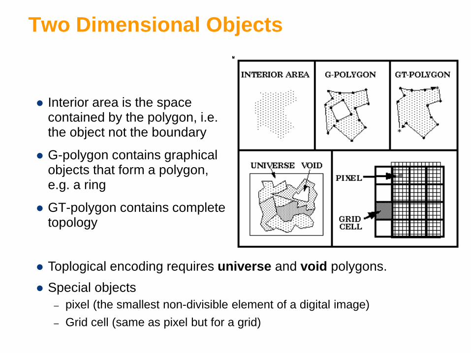
Two Dimensional Objects

Interior area is the space contained by the polygon, i.e. the object not the boundary

G-polygon contains graphical objects that form a polygon, e.g. a ring

GT-polygon contains complete topology

Toplogical encoding requires universe and void polygons. Special objects

– pixel (the smallest non-divisible element of a digital image) – Grid cell (same as pixel but for a grid)

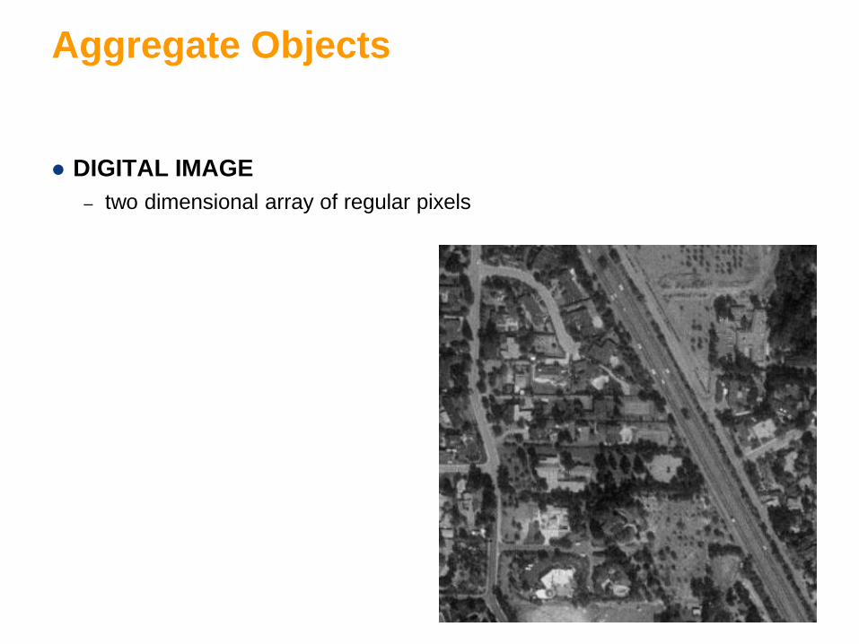
Aggregate Objects

DIGITAL IMAGE – two dimensional array of regular pixels

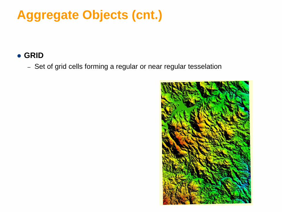
Aggregate Objects (cnt.)

GRID – Set of grid cells forming a regular or near regular tesselation

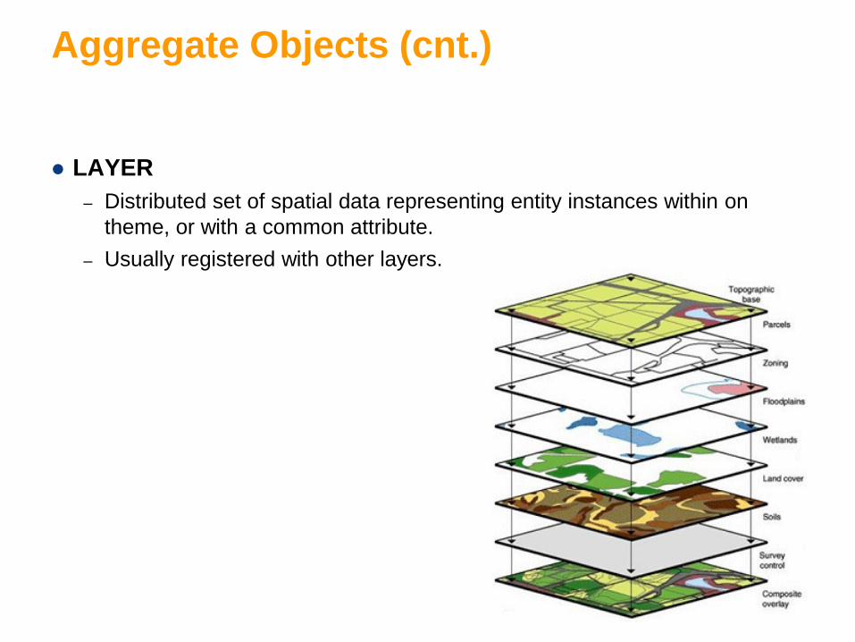
Aggregate Objects (cnt.)

LAYER – Distributed set of spatial data representing entity instances within on

theme, or with a common attribute. – Usually registered with other layers.

Aggregate Objects (cnt.)

RASTER – One or more overlapping layers from the same grid or digital image.

Red Green Blue

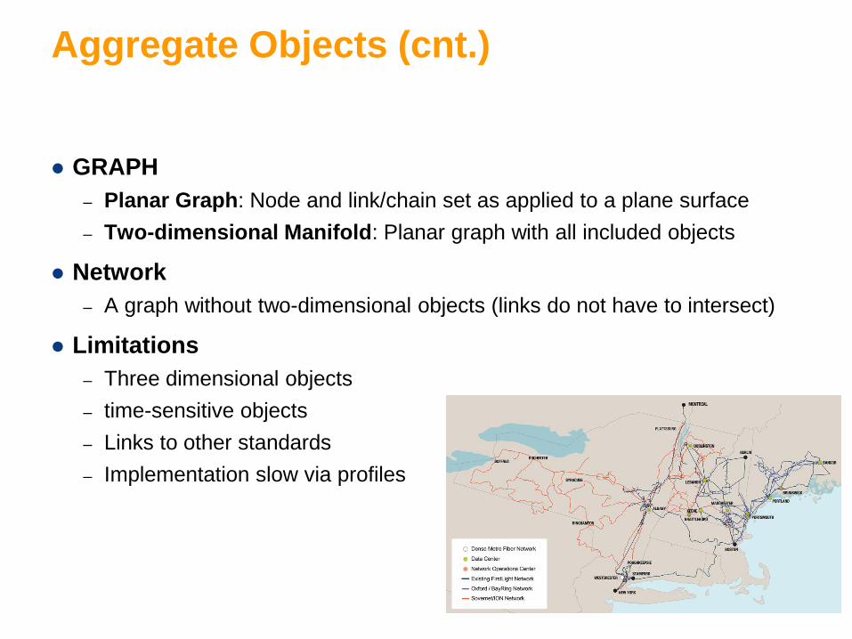
Aggregate Objects (cnt.)

GRAPH – Planar Graph: Node and link/chain set as applied to a plane surface – Two-dimensional Manifold: Planar graph with all included objects

Network – A graph without two-dimensional objects (links do not have to intersect)

Limitations – Three dimensional objects – time-sensitive objects – Links to other standards – Implementation slow via profiles

Summary

Map data structures are often input determined

Raster vs vector: strengths and weaknesses

Map data structures have corresponding programming data structures

Tour of data structures: entity-by-entity, point/line/area, raster/vector

TINS, networks and tesselations

Standards: old and new

Need to create aggregate objects