Embed Size (px)
Citation preview

JOURNAL OF FINANCIAL AND QUANTITATIVE ANALYSIS Vol. 48, No. 5, Oct. 2013, pp. 1573–1605COPYRIGHT 2013, MICHAEL G. FOSTER SCHOOL OF BUSINESS, UNIVERSITY OF WASHINGTON, SEATTLE, WA 98195doi:10.1017/S0022109013000562
Analyst Coverage, Information, and Bubbles
Sandro C. Andrade, Jiangze Bian, and Timothy R. Burch∗
Abstract
We examine the 2007 stock market bubble in China. Using multiple measures of bubbleintensity for each stock, we find significantly smaller bubbles in stocks for which there isgreater analyst coverage. We further show that the abating effect of analyst coverage onbubble intensity is weaker when there is greater disagreement among analysts. This sug-gests that, in line with resale option theories of bubbles, one channel through which analystcoverage may mitigate bubbles is by coordinating investors’ beliefs and thus reducing itsdispersion. Stock turnover provides further evidence consistent with this particular infor-mation mechanism.
I. Introduction
What is peculiar about China’s stock market is that government of-ficials, the People’s Bank of China, the media, investment bankers,not to mention Li Ka-shing, Hong Kong’s richest tycoon, and AlanGreenspan, the former chairman of the Federal Reserve, have all warnedthat it looks like a bubble. The Economist, May 24, 2007
Many [Chinese investors] try to educate themselves, poring over analystreports available free of charge at Web sites such as Hexun and China-stock. Business Week, March 19, 2007
∗Andrade, [email protected], Burch, [email protected], School of Business Administration,University of Miami, PO Box 248094, Coral Gables, FL 33124; and Bian, [email protected],School of Banking and Finance and Research Center for Applied Finance, University of InternationalBusiness and Economics, 908 Boxue Building, #10, HuixinDongjie, Beijing 100029, China. For use-ful comments, we are grateful to Brad Barber, Hendrik Bessembinder (the editor), Utpal Bhattacharya(discussant), Kalok Chan (the referee), Vidhi Chhaochharia, Marcelo Fernandes, David Hirshleifer,Li Jin (discussant), Alok Kumar, Robin Lumsdaine, Dhananjay Nanda, Tom Noe, Tao Shu, JonathanWang, Peter Wysocki, and seminar participants at American University, Florida Atlantic University,the 2010 Miami Behavioral Finance Conference, the 2010 Singapore International Conference onFinance, the 2011 Annual Chinese Finance Meeting, Queen Mary University of London, and theUniversity of Miami. Bian acknowledges support by the MOE (Ministry of Education in China)Liberal Arts and Social Sciences Foundation (Project No. 12YJC790001), the National Social ScienceFoundation of China (Project No. 12CJY117), and the Program for Innovative Research Team andProject 211 at the University of International Business and Economics. Early versions of this paperwere titled “Does Information Dissemination Mitigate Bubbles?”
1573

1574 Journal of Financial and Quantitative Analysis
Asset pricing bubbles are intriguing, large-scale economic phenomena. Thedistorted prices and potential resource misallocation associated with bubbles canlead to large societal costs. Bernanke (2002) notes the importance of understand-ing the factors that influence bubbles in order to design policies to mitigate suchphenomena, and the recent boom and collapse in real estate prices has generatedmuch debate among policy makers (Landau (2009), Bernanke (2010), and Dudley(2010)).
The anti-bubble policy prescriptions currently considered tend to be macroin nature. For example, discussions involve whether central banks should tightenmonetary policy in response to perceived asset bubbles, or which kind of macro-prudential regulations (tightening of capital requirements, imposing transactiontaxes or direct lending constraints, etc.) are likely to be most effective in deflatingbubbles.1 In contrast, this paper investigates whether a micro-level policy couldpotentially help mitigate asset pricing bubbles and thus complement macro-levelpolicies. In particular, we study whether greater dissemination of public informa-tion about an asset could lower its susceptibility to bubbles.
Theory suggests that dissemination of public information could mitigate bub-bles by coordinating investors’ beliefs. In resale option theories, bubbles arisethrough the interaction of belief dispersion and short-sale constraints (Harrisonand Kreps (1978), Scheinkman and Xiong (2003)).2 In these theories, investorshold beliefs that are correct on average. Nonetheless, investors knowingly paymore for an asset than the present value of future dividends in hopes of selling theasset at yet higher prices to more optimistic investors in the future. In the resaleoption framework, public dissemination of information could coordinate beliefsas all investors update their beliefs toward the valuation implied by informationbeing disseminated. Such coordination would thus lower bubble magnitude byreducing future belief dispersion and thereby the possibility that investors couldsell in the future to more optimistic investors. In Appendix A, we add public dis-semination of information to a two-period, two-state version of Scheinkman andXiong’s model in order to illustrate this bubble-mitigating mechanism. We showthat the stronger is the public information signal, the smaller is the asset pricebubble.
It is also possible that dissemination of public information mitigates bubblesby reducing investors’ overoptimism. In contrast to resale option theories of bub-bles, in which investors hold correct beliefs on average, bubbles may be causedby investors’ “irrational exuberance” (Shiller (2005), Han and Kumar (2013)).
1For discussion of macro-level bubble-mitigating policies, see Allen and Carletti (2011),Christensson, Spong, and Wilkinson (2011), and Prasad (2010). Known drawbacks to such macroapproaches include the need to recognize bubbles in real time in order to calibrate policy response andthe potential to create distortions in regions or markets without bubbles. Moreover, even if an assetbubble is identified in real time, the effectiveness of macro approaches is still open to question. Allen(2011) notes that evidence from Korea, Hong Kong, and Singapore suggests that macro-prudentialmeasures aiming at eliminating real estate bubbles may work in the short run but not in the long run.
2In addition to the dynamic resale option theories of bubbles, several static theories also feature apositive price bias due to the interaction between the dispersion of beliefs across investors and short-sale constraints (e.g., Miller (1977), Chen, Hong, and Stein (2002)). However, static models do notcapture the speculative trading (buying in anticipation of capital gains, rather than buying and holdingin order to receive long-term income streams) that is often ascribed to bubbles.

Andrade, Bian, and Burch 1575
If that is the case, public information could serve as a “reality check” that anchorsbeliefs to fundamentals.3
To pursue our research question, we need a plausibly identified market-widebubble and measures of the intensity of the bubble and of the degree of publicdissemination of information in each individual asset in the bubble. The 2007stock market in China provides an ideal setting. As we explain in Section II, the2007 Chinese stock market displays classic features of a bubble, including a boomfollowed by a bust in asset prices, a dramatic surge in trading activity that isstrongly correlated with price levels, and a documented flood of novice investorsentering the market. Moreover, the Chinese setting allows us to construct uniquemeasures of bubble intensity in individual assets, measures that are not available,for example, when studying the U.S. Internet bubble of the late 1990s.4 Theseunique measures collectively alleviate concerns about measurement error.
Following an extensive literature, we use the number of security analystscovering a stock as a measure of the degree of public dissemination of informa-tion.5 Analysts are specialized professionals who collect information about stocksand disseminate it to market participants in the form of periodic reports, earningsforecasts, and buy/sell/hold recommendations. To the extent that analyst researchis at least partially independent and not released at the same time, a greater num-ber of analysts producing and disseminating research about a given stock shouldresult in a higher rate of information flow to market participants.
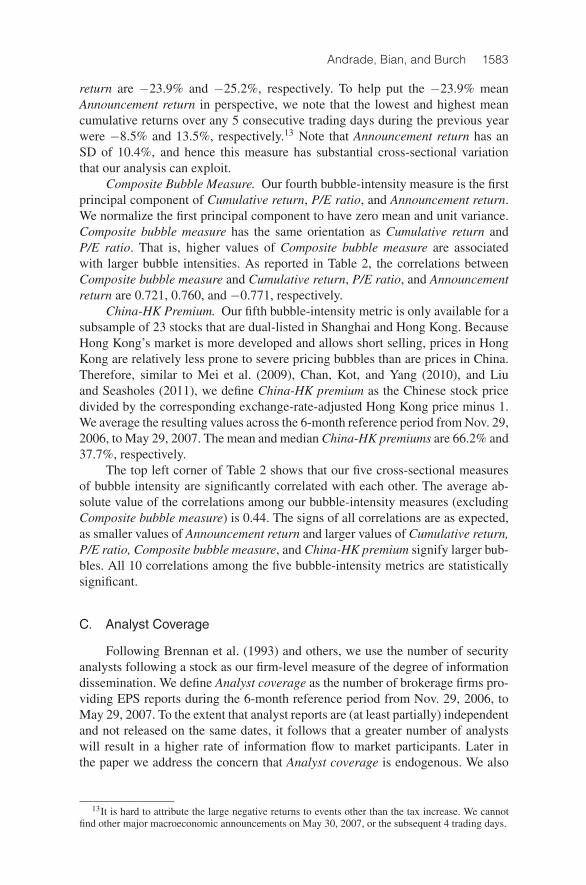
Figure 1 illustrates our key finding: Stocks with less analyst coverage de-velop significantly larger bubbles. On the vertical axis, we plot Composite bubblemeasure, one of our five measures of the intensity of the bubble in each individualstock. This measure is normalized to have a mean of 0 and a standard deviation(SD) equal to 1, and therefore a negative Composite bubble measure does notimply a negative bubble, just a bubble intensity that is below the cross-sectionalaverage. On the horizontal axis, we plot Analyst coverage, the number of analystsfollowing a stock. Figure 1 shows there is a strong negative correlation betweeneach stock Composite bubble measure and its Analyst coverage. Results are simi-lar when we use any of the other four bubble-intensity measures in our study.
We show that the negative correlation between Analyst coverage and bubbleintensity remains after controlling for several stock-level characteristics. In par-ticular, we provide compelling evidence that our key finding is not driven by the
3Note there is a subtle but important difference between these two bubble-mitigating mechanisms.The overoptimism reduction channel mechanism requires that the public information being dissemi-nated is truly informative, whereas the belief coordination channel only requires that it is perceivedto be informative. Hence, even though stock analyst research may suffer from an assortment of biases(e.g., De Bondt and Thaler (1990), Ertimur, Muslu, and Zhang (2011)), it could nevertheless mitigatebubbles as long as investors deem it credible.
4In preliminary results we apply a similar research design to the U.S. Internet bubble of the late1990s and find similar results: All else being equal, bubbles are smaller when there is more analystcoverage. Results are available from the authors.
5A partial list of papers using analyst coverage as a measure of the quality of the information en-vironment includes Brennan, Jegadeesh, and Swaminathan (1993), Hong, Lim, and Stein (2000), Houand Moskowitz (2005), Chan and Hameed (2006), Duarte, Han, Harford, and Young (2008), Kumar(2009), Hong and Kacperczyk (2010), and Kelly and Ljungqvist (2012). Ganguli and Yang (2009) andAngeletos and Werning (2006) investigate other dimensions of how the supply of information affectsfinancial markets.

1576 Journal of Financial and Quantitative Analysis
FIGURE 1
Bubble Intensity and Analyst Coverage
Figure 1 shows a scatter plot of Composite bubble measure, one of our measures of the bubble intensity for each stock,and Analyst coverage. Composite bubble measure is normalized to have a mean of 0 and a variance equal to 1. The R2
of the best fit line is equal to 0.46. The sample consists of 623 Shanghai A-shares.
well-known fact that larger stocks tend to attract more analyst coverage coupledwith the possibility that larger stocks also develop smaller bubbles for reasonsunrelated to analyst coverage.
The results also show that analyst coverage is less effective in reducing bub-ble intensity when there is greater disagreement among analysts, measured bythe dispersion of earnings forecasts or dispersion of buy/sell recommendations(or their first principal component).6 This finding is important for two reasons.First, it alleviates concerns that Analyst coverage is correlated with bubble in-tensity solely because both variables are determined by a third, stock-specificvariable orthogonal to all our control variables. If that was the case, then howanalysts disseminate the information (with more or less disagreement) should beirrelevant.7 Second, it provides insight as to why analyst coverage mitigates bub-bles. Specifically, it supports the idea that analyst coverage mitigates bubbles bycoordinating investors’ beliefs. This is because analyst coverage should be less
6Note that disagreement among analysts is not necessarily a good proxy for disagreement amonginvestors in China. This market is dominated by retail investors who are more likely to display over-confidence in the Scheinkman and Xiong (2003) sense (i.e., focusing on a limited, idiosyncratic infor-mation set, and overestimating the validity of the approaches they use to value stocks). Nonetheless,disagreement among analysts is useful in our analysis because it plausibly regulates the degree towhich a given amount of analyst coverage is able to coordinate investors’ beliefs. For a given numberof analysts following a stock, the information that they disseminate should be less effective in coordi-nating investors’ beliefs (and hence mitigating bubbles) when analysts themselves disagree more.
7Three additional exercises further address endogeneity concerns. First, in Section IV.B.1 we showthat analyst coverage in 2005 (well before the bubble developed) is also negatively correlated withbubble intensity during 2007. Second, instrumental variables regressions in Section IV.B.2 corrobo-rate the negative association between bubble intensity and analyst coverage. Third, in Section VI.Bwe explicitly provide evidence against three specific alternative stories based on endogenous analystcoverage.

Andrade, Bian, and Burch 1577
effective in coordinating investors’ beliefs when stock analysts themselves havemore dispersed beliefs.
We provide further evidence consistent with analyst coverage mitigatingbubbles by coordinating beliefs and thus reducing belief dispersion across in-vestors. Even though we cannot directly observe the dispersion of beliefs acrossinvestors (as opposed to dispersion among analysts), several theories indicate thatit is positively related to stock turnover. We show that Analyst coverage is neg-atively associated with stock turnover, consistent with analyst research coordi-nating beliefs across investors. Furthermore, analogous to our empirical analysisexplaining bubble intensities, we find that the abating effect of Analyst coverageon stock turnover is weaker when there is more disagreement among analysts.This is an additional result one would expect if analyst coverage is indeed lesseffective in coordinating beliefs when there is more disagreement among analyststhemselves.
For completeness, we investigate the possibility that analyst coverage miti-gates bubbles by reducing investor overoptimism, in addition to reducing beliefdispersion. We find that there is very little time-series variation in the averageanalyst recommendation before, during, and after the bubble. If anything, the av-erage recommendation becomes slightly more optimistic as the bubble inflates.This indicates that analysts do not lean against high valuations during the bubble,and that analyst coverage does not mitigate bubbles by reducing investor overop-timism in our setting.
Overall, we find that stocks with more analyst coverage are much less af-fected by the spectacular boom and bust of the Chinese stock market in 2007.Multiple findings support an information-based channel in which analyst cover-age mitigates bubbles by coordinating investors’ beliefs. Thus, our results suggestthat policies that increase public information dissemination to market participantsmay help mitigate asset pricing bubbles.
II. Why Study China?
There are at least three reasons why the 2007 Chinese stock market pro-vides a good empirical setting in which to study asset pricing bubbles. First, theChinese stock market has institutional characteristics that are conducive to bub-bles. Specifically, like residential real estate markets around the world, the Chi-nese stock market is dominated by retail investors and has very strict short-sellingconstraints. Bailey, Cai, Cheung, and Wang (2009) document that individual in-vestors accounted for 92% of the trading volume in 198 large Chinese stocks fromOct. 2003 to March 2004. Moreover, during 2007 short sales were forbidden,and the ability of pessimistic investors to indirectly affect equity prices through aderivatives market was extremely limited.8
Second, the 2007 Chinese stock market displays classic features of a bubble:a boom followed by a bust in asset prices, a dramatic surge in trading activitythat is strongly correlated with asset price levels, and a flood of novice investors
8There were put warrants during our sample period, but these contracts only existed for a tinysubset of stocks.

1578 Journal of Financial and Quantitative Analysis
entering the market (Kindleberger and Aliber (2005), Cochrane (2003), Hong andStein (2007), and Greenwood and Nagel (2009)). Note that the Economist quoteopening our paper shows that many recognized the 2007 bubble even before itcrashed. Thus, any ex post rationalization for the boom and bust in asset pricesand trading activity has to contend with such pre-crash views.
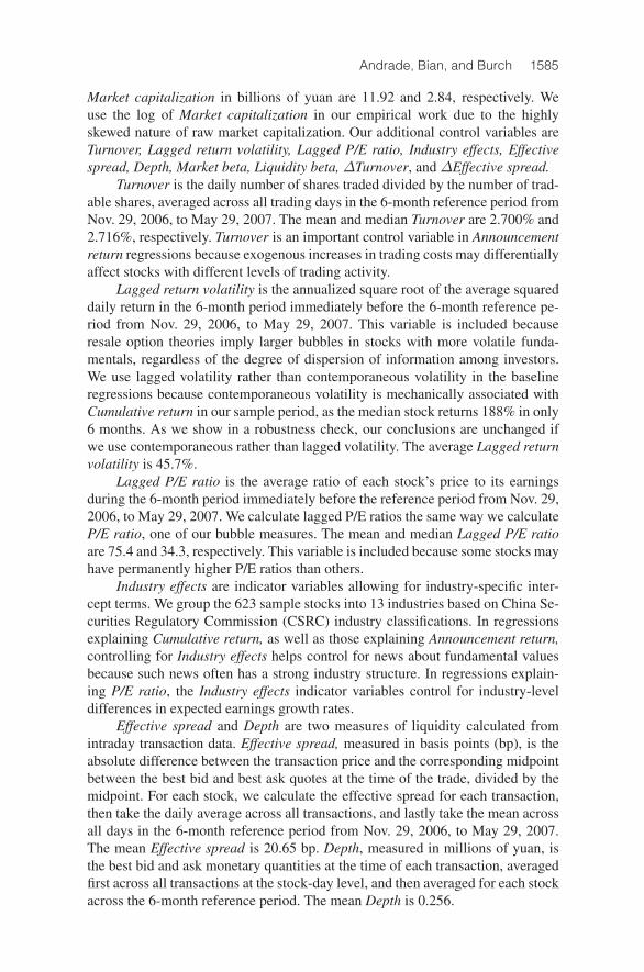
Figure 2 illustrates key elements of the bubble. Graph A plots the evolutionof the median price/earnings (P/E) ratio and the median daily turnover acrossShanghai A-shares in our sample. During the 6-month period from Nov. 29, 2006,to May 29, 2007, the median stock in our sample has its P/E ratio increase from35 to 85, and its annualized daily turnover increases from 230% to 950%. As thefigure shows, both P/E ratios and turnover decline after May 30, 2007, eventuallyfalling to 20 and 150%, respectively, by Oct. 2008. The correlation between P/Eratios and turnover over the entire Jan. 2005 to Dec. 2008 period is 0.70. Graph Bplots cumulative returns of the value-weighted Shanghai stock market index inrolling 6-month windows. During the 6-month period from Nov. 29, 2006, toMay 29, 2007, the Shanghai stock index has a cumulative return equal to 178%,which is the highest 6-month return in the 2000–2010 period (Figure 2 only shows2005–2009).
FIGURE 2
The Chinese Stock Market Bubble of 2007
Figure 2 illustrates key elements of the Chinese stock market bubble of 2007. All graphs show variables over the Jan. 2005–Jan. 2009 time period. Graph A has the median P/E ratio (left axis) and the median daily annualized stock turnover (rightaxis) of the 623 Shanghai A-shares in our sample. Graph B has the cumulative stock returns over the previous 6-monthperiod of our sample stocks. Graph C shows a weekly index that tracks the relative level of Google searches for the terms“stock” or “stock market” (in Chinese) relative to overall Google searches in China. Graph D shows the monthly number ofnew (A-share) trading accounts opened in the Shanghai Stock Exchange.
Graph A. Median P/E and Turnover Graph B. Value-Weighted 6-Month Returns
Graph C. Google Searches in China Graph D. New Trading Accounts

Andrade, Bian, and Burch 1579
Alongside soaring asset prices and trading activity, from Dec. 2006 to May2007 a total of 7.8 million new retail-investor A-share trading accounts werecreated at brokerages trading on the Shanghai Stock Exchange (see Graph D ofFigure 2). These data are from the Shanghai Stock Exchange. The new accountsrepresent a 21% increase in the total number of retail A-share accounts duringjust 6 months. Because individual investors were not allowed to open accountsin multiple brokerages, the surge in new accounts is overwhelmingly due to newindividual investors venturing into a booming equity market.
Graph C of Figure 2 plots a weekly index measuring the number of Googlesearches that originate in China for the terms “stock” or “stock market” (inChinese), relative to overall Google search volume originating in China. The in-dex is provided by Google Insights for Search and is normalized to 100 at thesample period peak. The plot shows a fivefold increase in Google searches fromDec. 2006 to May 2007, with a peak in the week of May 30, 2007, and almostmonotonic decline thereafter. Google search data thus confirm that the 2007 Chi-nese stock market was marked by unusually high retail-investor interest, consis-tent with the flood of novice investors opening A-share trading accounts.
The third and arguably most important reason that the 2007 Chinese stockmarket offers an attractive setting is because it allows us to construct several stock-specific bubble-intensity measures (some of them unique) that collectively helpovercome measurement error concerns. These measures, discussed in detail inSection III, are cumulative returns, P/E ratios, announcement returns following asudden tripling of China’s security transaction tax, the first principal componentof these aforementioned metrics (labeled Composite bubble measure), and theratios of prices in China over prices in Hong Kong for a subsample of stocks listedin both markets. Although none of these bubble-intensity measures is perfect,they are all reasonable proxies and at least to some extent provide conceptuallyindependent measures of overvaluation. Thus, finding consistent results using allof these proxies would increase confidence in our conclusions.
III. Data and Variables
Our sample consists of the 623 Shanghai A-share stocks that traded on atleast 90% of the trading days during the 6-month period from Nov. 29, 2006, toMay 29, 2007. All of our data are from RESSET, a major provider of Chinesefinancial data.9 RESSET obtains its stock market data directly from the stockexchanges. Similar to Institutional Brokers’ Estimate System (IBES), RESSETcollects its analyst forecast data from brokerage firms, except that the RESSETanalyst database is much more comprehensive than the IBES data set for China.10
The brokerage firms in the RESSET data issuing reports and earnings per share
9RESSET is headquartered at Tsinghua University. For more information, please see http://www.resset.cn/en/.
10Specifically, 250 of our sample stocks are reported with at least one analyst in the IBES data,whereas 453 stocks have at least one analyst covering them according to the RESSET data. The cor-relation between IBES analyst coverage and RESSET analyst coverage is 0.78. The Online Appendix(http://moya.bus.miami.edu/∼sandrade/research.html) shows that our results are robust to using IBESanalyst coverage for China rather than the RESSET analyst coverage.

1580 Journal of Financial and Quantitative Analysis
(EPS) forecasts for our sample stocks are listed in the Online Appendix. Tables 1and 2 report summary statistics for the main variables in this study.
TABLE 1
Summary Statistics
Table 1 reports summary statistics for the main variables in the study. The variables are described in Table B1 of AppendixB. The sample consists of 623 Shanghai A-shares, selected by requiring that shares be traded on at least 90% of thetrading days in the reference period. The reference period is from Nov. 29, 2006, to May 29, 2007.
Variables Mean Median Std. Dev.
Cumulative return (%) 204.4 187.6 95.2P/E ratio 94.2 56.7 79.2Announcement return (%) −23.9 −25.2 10.4Composite bubble measure 0.000 −0.065 1.000China-HK premium (%) 66.2 37.7 63.4Analyst coverage 6.07 3.00 7.07Market capitalization (billions of yuans) 11.92 2.84 70.54Log of market capitalization 1.271 1.045 1.077Turnover (daily, in %) 2.700 2.716 1.239Lagged return volatility (annualized, %) 45.7 43.7 12.9Lagged P/E ratio 75.4 34.3 81.5Effective spread (bp) 20.65 20.00 5.45Depth (millions of yuans) 0.256 0.172 0.450Market beta 0.963 0.984 0.218Liquidity beta −0.116 −0.129 0.295ΔTurnover (daily, in %) −0.697 −0.641 0.638ΔEffective spread (bp) −1.519 −1.598 4.306
A. The Reference Period
Our analysis requires us to define a period over which to compute bubble-intensity measures, analyst coverage, and the control variables. In our baselineresults we adopt a 6-month reference period from Nov. 29, 2006, to May 29,2007. Figure 2 suggests a reference period ending May 29, 2007, based on P/Eratios, turnover, cumulative returns, and two measures of retail-investor enthusi-asm (Google searches and account openings). Moreover, on May 30, 2007, theChinese government implemented a previously unannounced tripling of China’ssecurity transaction tax, which seemingly marked a regime change in the Chinesestock market. We show later that our results are robust to using different windowlengths ending on May 29, 2007, and that our results do not obtain in placebo6-month periods far from May 30, 2007. For completeness, our Online Appendixplots price indices levels for our sample stocks.
B. Measures of Bubble Intensity
Cumulative Return. This variable is the cumulative stock return during the6-month reference period from Nov. 29, 2006, to May 29, 2007. As reported inTable 1, the mean and median of Cumulative return are 204.4% and 187.6%,respectively, implying that the average stock roughly tripled in price over the 6-month reference period. Of the 623 sample stocks, 567 (91%) have Cumulativereturn exceeding 100%, 275 (44%) have returns exceeding 200%, and 73 (12%)have returns exceeding 300%. The smallest Cumulative return is 53%.
P/E Ratio. This variable is the average ratio of each stock’s price to itsearnings during the 6-month reference period from Nov. 29, 2006, to May 29,2007. Each day, we calculate this ratio using the total earnings reported over the

And
rade,B
ian,andB
urch1581
TABLE 2
Correlation Matrix
Table 2 reports correlation coefficients between the main variables of this study. The variables are described in Table B1 of Appendix B. The sample consists of 623 Shanghai A-shares, selected by requiring thatshares be traded on at least 90% of the trading days in the reference period. The reference period is from Nov. 29, 2006, to May 29, 2007.
Com
p.B
ubb
leM
eas.
Cum
ulat
ive
Ret
urn
P/E
Rat
io
Ann
ounc
emen
tRet
urn
Chi
na-H
KP
rem
ium
Ana
lyst
Cov
erag
e
Log
ofM
arke
tCap
.
Turn
over
Lag
ged
Ret
urn
Vol
.
Lag
ged
P/E
Rat
io
Effe
ctiv
eS
pre
ad
Dep
th
Mar
ketB
eta
Liq
uid
ityB
eta
ΔTu
rnov
er
ΔE
ffect
ive
Sp
read
Comp. bubble meas. 1.000Cumulative return 0.721 1.000P/E ratio 0.760 0.316 1.000Announcement return –0.771 –0.334 –0.390 1.000China-HK premium 0.679 0.482 0.661 –0.481 1.000Analyst coverage –0.685 –0.400 –0.455 0.679 –0.691 1.000Log of market cap. –0.484 –0.186 –0.347 0.547 –0.499 0.754 1.000Turnover 0.506 0.353 0.265 –0.518 0.434 –0.514 –0.504 1.000Lagged return vol. 0.167 0.010 0.315 –0.048 0.551 –0.189 –0.156 0.066 1.000Lagged P/E ratio 0.676 0.269 0.923 –0.318 0.607 –0.403 –0.304 0.220 0.320 1.000Effective spread 0.516 0.349 0.518 –0.295 0.225 –0.418 –0.443 0.057 0.115 0.478 1.000Depth –0.135 –0.056 –0.081 0.163 –0.270 0.342 0.575 –0.097 –0.162 –0.062 –0.073 1.000Market beta –0.047 0.127 –0.237 –0.013 –0.261 0.111 0.195 0.196 –0.051 –0.219 –0.349 0.096 1.000Liquidity beta 0.053 0.169 –0.053 –0.012 –0.380 0.099 0.213 0.004 –0.090 –0.025 –0.050 0.217 0.529 1.000ΔTurnover –0.138 –0.071 –0.059 0.179 –0.348 0.116 0.155 –0.632 –0.072 –0.053 0.082 –0.015 –0.161 0.030 1.000ΔEffective spread –0.286 –0.488 –0.115 0.058 0.194 0.029 –0.197 –0.071 0.124 –0.011 –0.323 –0.186 –0.108 –0.157 –0.168 1.000

1582 Journal of Financial and Quantitative Analysis
four most recent available quarterly earnings prior to the calculation date. We capdaily P/E ratios at 250 and assign a P/E ratio of 250 to stocks with negative earn-ings. We then compute the average ratio for each stock throughout the referenceperiod. The mean and median P/E ratios are 94.2 and 56.7, respectively.
Announcement Return. Even though Cumulative return and P/E ratio areintuitive measures that capture cross-sectional differences in bubble intensities,both are noisy. As an alternative stock-specific measure of bubble intensity, weexploit our unique setting to construct a third metric that we label Announcementreturn. We argue that this measure should be less affected by unobservable cross-sectional variation in the evolution of fundamentals and in earnings growth rates.
Announcement return is each stock’s 5-day cumulative return following theannouncement of the tripling of China’s security transaction tax on May 30, 2007.Before the market’s open on this day, the Chinese government announced and im-plemented a sudden increase in the security transaction tax from 0.1% to 0.3%.News reports suggest the tax increase was motivated by concerns over an over-heating stock market.
We argue that stocks with larger bubbles would have had stronger price re-actions to this sudden tax increase. This bubble-intensity identification strategy isanchored on Scheinkman and Xiong’s (2003) theory of bubbles, which impliesthat prices of stocks in larger bubbles will have more negative price reactionsto an increase in trading costs.11 In their theory, asset prices have two compo-nents: a fundamental value given by the expected present value of future dividends(averaged across different investors’ beliefs), plus the value of the option to resellto potential future investors at greater prices. Scheinkman and Xiong show that anincrease in trading costs instantly decreases the value of the resale option (whichdepends on expected after-tax cash flows of future stock trading). This impliesthat stocks in which the resale option is a larger fraction of the stock price shouldhave larger percentage price decreases in response to the transaction tax increaseannouncement.12
The 5-day period in the calculation of Announcement return starts on May30, 2007, because the tax tripling announcement was made early that day beforethe market opened. We use 5-day returns because China has a price change limitof 10% per day, and many stocks hit the limit on one or more of the first 4 daysfollowing the tax increase announcement (as detailed later, results are robust toshorter and longer windows). For example, 122 stocks have −10% returns on allof the first 3 days following the tax increase. The mean and median Announcement
11Mei, Scheinkman, and Xiong (2009) and Xiong and Yu (2011) find evidence supporting theresale option theory of bubbles in Chinese securities markets. However, our strategy of identifyingbubble intensities through Announcement return is also consistent with investors viewing the suddentax tripling as a strong, public signal from the Chinese government that the market was overvalued,which could also reduce bubble magnitudes.
12Suppose that stocks H and L are priced at $100, and that the fundamental values of H and L are$50 and $90, respectively. Thus, the bubble intensity of stock H is five times larger than the bubbleintensity of stock L. A common security transaction tax increase levied on both stocks implies thatthe value of the option to resell decreases by a similar proportion in both stocks, say, 50%. Such adecrease would imply post-tax-increase announcement prices of about $75 and $95 for stocks H andL, respectively, leading to announcement returns of −25% and −5%. Note that these announcementreturns are proportional to bubble intensities in this simple example.
Andrade, Bian, and Burch 1583
return are −23.9% and −25.2%, respectively. To help put the −23.9% meanAnnouncement return in perspective, we note that the lowest and highest meancumulative returns over any 5 consecutive trading days during the previous yearwere −8.5% and 13.5%, respectively.13 Note that Announcement return has anSD of 10.4%, and hence this measure has substantial cross-sectional variationthat our analysis can exploit.
Composite Bubble Measure. Our fourth bubble-intensity measure is the firstprincipal component of Cumulative return, P/E ratio, and Announcement return.We normalize the first principal component to have zero mean and unit variance.Composite bubble measure has the same orientation as Cumulative return andP/E ratio. That is, higher values of Composite bubble measure are associatedwith larger bubble intensities. As reported in Table 2, the correlations betweenComposite bubble measure and Cumulative return, P/E ratio, and Announcementreturn are 0.721, 0.760, and −0.771, respectively.
China-HK Premium. Our fifth bubble-intensity metric is only available for asubsample of 23 stocks that are dual-listed in Shanghai and Hong Kong. BecauseHong Kong’s market is more developed and allows short selling, prices in HongKong are relatively less prone to severe pricing bubbles than are prices in China.Therefore, similar to Mei et al. (2009), Chan, Kot, and Yang (2010), and Liuand Seasholes (2011), we define China-HK premium as the Chinese stock pricedivided by the corresponding exchange-rate-adjusted Hong Kong price minus 1.We average the resulting values across the 6-month reference period from Nov. 29,2006, to May 29, 2007. The mean and median China-HK premiums are 66.2% and37.7%, respectively.
The top left corner of Table 2 shows that our five cross-sectional measuresof bubble intensity are significantly correlated with each other. The average ab-solute value of the correlations among our bubble-intensity measures (excludingComposite bubble measure) is 0.44. The signs of all correlations are as expected,as smaller values of Announcement return and larger values of Cumulative return,P/E ratio, Composite bubble measure, and China-HK premium signify larger bub-bles. All 10 correlations among the five bubble-intensity metrics are statisticallysignificant.
C. Analyst Coverage
Following Brennan et al. (1993) and others, we use the number of securityanalysts following a stock as our firm-level measure of the degree of informationdissemination. We define Analyst coverage as the number of brokerage firms pro-viding EPS reports during the 6-month reference period from Nov. 29, 2006, toMay 29, 2007. To the extent that analyst reports are (at least partially) independentand not released on the same dates, it follows that a greater number of analystswill result in a higher rate of information flow to market participants. Later inthe paper we address the concern that Analyst coverage is endogenous. We also
13It is hard to attribute the large negative returns to events other than the tax increase. We cannotfind other major macroeconomic announcements on May 30, 2007, or the subsequent 4 trading days.

1584 Journal of Financial and Quantitative Analysis
present evidence consistent with an information channel explaining the link wefind between Analyst coverage and bubble intensity.
In line with Chan and Hameed (2006), we argue that analyst coverage is aparticularly good cross-sectional measure of information dissemination in China.Compared to markets such as the United States, the corporate environment inChina has a relatively low degree of voluntary disclosure and transparency. It ispresumably more difficult for Chinese investors to observe and analyze relevantfirm information on their own, and such investors are likely to seek guidance fromanalyst reports, as the paper’s second opening quote indicates.
Chinese investors can obtain analyst reports from the brokerage firms inwhich they have stock brokerage accounts. Moreover, a few popular Web sitesserve as repositories for analyst reports from different brokerage firms (e.g.,www.cnstock.com and www.prnews.cn/rating). Analyst reports are even avail-able in the finance sections of popular Web portals such as www.sina.com.cn andwww.sohu.com. Finally, summaries of analyst reports and recommendations arealso available in nationally circulated financial newspapers such as Shanghai Se-curities News and China Securities Journal.
Consistent with the notion that analyst reports matter for Chinese investors,Moshirian, Ng, and Wu (2009) find that between 1996 and 2005, Chinese stockprices react to changes in analyst buy/sell recommendations. In our sample, wefind that the average 3-day market-adjusted reaction to a strong upward revision(e.g., from hold to strong buy) exceeds that to a strong downgrade by an averageof 2.9%, with the average reaction to an upgrade statistically different than thereaction to a downgrade (p-value = 0.0002).14
Table 1 shows that the mean and median Analyst coverage are 6.07 and 3.00,respectively, and Table 2 shows that Analyst coverage is smaller when any of ourfive bubble-intensity metrics implies larger bubbles. The correlations between An-alyst coverage and Cumulative return, P/E ratio, Announcement return, Compos-ite bubble measure, and China-HK premium are −0.400, −0.455, 0.679, −0.685,and −0.691, respectively.
D. Control Variables
We include several control variables in our regressions explaining bubble-intensity measures. Although some of our control variables are more justified thanothers depending on the bubble-intensity measure under study, for simplicity theregression analyses include all of them regardless of the bubble-intensity metricused.
Market capitalization is the most important control variable in our analysis,because presumably larger firms are expected to attract more analysts, and yet sizemay be correlated with stock characteristics that are orthogonal to informationdissemination. We use the average market capitalization throughout the 6-monthreference period from Nov. 29, 2006, to May 29, 2007. The mean and median
14If we consider the reaction to any upgrade or downgrade, the announcement reaction to upgradesexceeds that to downgrades by 0.9%, on average, and the average reactions to upgrades and down-grades are statistically different, with a p-value of 0.010.
Andrade, Bian, and Burch 1585
Market capitalization in billions of yuan are 11.92 and 2.84, respectively. Weuse the log of Market capitalization in our empirical work due to the highlyskewed nature of raw market capitalization. Our additional control variables areTurnover, Lagged return volatility, Lagged P/E ratio, Industry effects, Effectivespread, Depth, Market beta, Liquidity beta,ΔTurnover, and ΔEffective spread.
Turnover is the daily number of shares traded divided by the number of trad-able shares, averaged across all trading days in the 6-month reference period fromNov. 29, 2006, to May 29, 2007. The mean and median Turnover are 2.700% and2.716%, respectively. Turnover is an important control variable in Announcementreturn regressions because exogenous increases in trading costs may differentiallyaffect stocks with different levels of trading activity.
Lagged return volatility is the annualized square root of the average squareddaily return in the 6-month period immediately before the 6-month reference pe-riod from Nov. 29, 2006, to May 29, 2007. This variable is included becauseresale option theories imply larger bubbles in stocks with more volatile funda-mentals, regardless of the degree of dispersion of information among investors.We use lagged volatility rather than contemporaneous volatility in the baselineregressions because contemporaneous volatility is mechanically associated withCumulative return in our sample period, as the median stock returns 188% in only6 months. As we show in a robustness check, our conclusions are unchanged ifwe use contemporaneous rather than lagged volatility. The average Lagged returnvolatility is 45.7%.
Lagged P/E ratio is the average ratio of each stock’s price to its earningsduring the 6-month period immediately before the reference period from Nov. 29,2006, to May 29, 2007. We calculate lagged P/E ratios the same way we calculateP/E ratio, one of our bubble measures. The mean and median Lagged P/E ratioare 75.4 and 34.3, respectively. This variable is included because some stocks mayhave permanently higher P/E ratios than others.
Industry effects are indicator variables allowing for industry-specific inter-cept terms. We group the 623 sample stocks into 13 industries based on China Se-curities Regulatory Commission (CSRC) industry classifications. In regressionsexplaining Cumulative return, as well as those explaining Announcement return,controlling for Industry effects helps control for news about fundamental valuesbecause such news often has a strong industry structure. In regressions explain-ing P/E ratio, the Industry effects indicator variables control for industry-leveldifferences in expected earnings growth rates.
Effective spread and Depth are two measures of liquidity calculated fromintraday transaction data. Effective spread, measured in basis points (bp), is theabsolute difference between the transaction price and the corresponding midpointbetween the best bid and best ask quotes at the time of the trade, divided by themidpoint. For each stock, we calculate the effective spread for each transaction,then take the daily average across all transactions, and lastly take the mean acrossall days in the 6-month reference period from Nov. 29, 2006, to May 29, 2007.The mean Effective spread is 20.65 bp. Depth, measured in millions of yuan, isthe best bid and ask monetary quantities at the time of each transaction, averagedfirst across all transactions at the stock-day level, and then averaged for each stockacross the 6-month reference period. The mean Depth is 0.256.

1586 Journal of Financial and Quantitative Analysis
Market beta and Liquidity beta are control variables capturing systematicfactor loadings. All else being equal, stocks with higher betas should have lowervalues of P/E ratio, larger values of Cumulative return, and more negative valuesof Announcement return. To estimate Market beta and Liquidity beta, we regressdaily stock returns during the 6-month reference period from Nov. 29, 2006, toMay 29, 2007, against the aggregate value-weighted market return and an aggre-gate liquidity factor. All of our results are robust to regressing stock returns on themarket and liquidity factors separately instead. For the liquidity factor, we use theinnovation in the average daily effective spread across all stocks, where each day’sinnovation is defined as the residual in a regression of the average effective spreadacross stocks on its lagged value, similar to Acharya and Pedersen (2005). For themarket factor, we use the value-weighted return on all tradable Shanghai A-shares.The mean Market beta is 0.963, and the mean Liquidity beta is −0.116.15
We use ΔTurnover and ΔEffective spread to control for changes in tradingactivity and trading costs following the tax increase on May 30, 2007.16 Thesevariables control for the possibility that each stock’s Announcement return par-tially reflects changes in an illiquidity discount as implied by models such as Lo,Mamaysky, and Wang (2004) and Acharya and Pedersen (2005). ΔTurnover isthe average daily turnover during the 6-month period immediately following the6-month reference period from Nov. 29, 2006, to May 29, 2007, minus the averagedaily turnover in the reference period. The definition ofΔEffective spread is anal-ogous. The meanΔTurnover andΔEffective spread are−0.697% and−1.519 bp,respectively.
IV. Analyst Coverage and Bubble Intensity
In Table 3 we report ordinary least squares (OLS) regressions of our fourfull-sample bubble-intensity measures onto Analyst coverage and various con-trol variables (we defer analysis using China-HK premium until Section IV.C).Columns (1), (3), (5), and (7) show that bubble measures are strongly corre-lated with Analyst coverage. The signs of the correlations indicate that stocks withlarger Analyst coverage experience smaller bubbles (i.e., lower Cumulative return,lower P/E ratio, higher (less negative) Announcement return, and lower Compos-ite bubble measure). The adjusted R2s of these univariate regressions range from0.16 in column (1) to 0.46 in columns (5) and (7).
Columns (2), (4), (6), and (8) show that the negative association betweenAnalyst coverage and bubble intensity remains after we add a battery of controlvariables. In all cases the coefficient on Analyst coverage is statistically significantat the 1% level. The coefficients in columns (2), (4), (6), and (8) are economically
15In robustness work available in our Online Appendix, we address the concern that Market betaand Liquidity beta, even though theoretically motivated, do not adequately represent true factor load-ings in the data (Ross (1976)). We replace Market beta and Liquidity beta with three empirical factorloadings constructed from a factor analysis of returns. Our conclusions are unchanged when we usethese empirical factor exposures in place of Market beta and Liquidity beta.
16In robustness work, we include aΔDepth variable, and all of our conclusions are unchanged. Wedo not includeΔDepth in our baseline specifications becauseΔDepth is very strongly correlated withDepth (ρ=−0.95).

Andrade, Bian, and Burch 1587
TABLE 3
Regressions Explaining Bubble-Intensity Measures
Table 3 reports ordinary least squares regressions that explain four stock-level bubble-intensity measures. The sampleconsists of 623 Shanghai A-shares, selected by requiring that shares be traded on at least 90% of the trading days inthe reference period. The reference period is from Nov. 29, 2006, to May 29, 2007. The variables are described in Ta-ble B1 of Appendix B. We report heteroskedasticity-robust t-statistics in parentheses below variable coefficients. ***, **,and * denote statistical significance at the 1%, 5%, and 10% levels, respectively.
Dependent Variables
Cumulative P/E Announcement CompositeReturn Ratio Return Bubble Measure
ExplanatoryVariables (1) (2) (3) (4) (5) (6) (7) (8)
Analyst –5.392*** –4.628*** –5.086*** –0.843*** 0.997*** 0.748*** –0.097*** –0.058***coverage (–13.37) (–7.56) (–15.91) (–3.59) (21.46) (9.88) (–26.84) (–12.00)
Log of market 28.228*** 9.455*** 0.592 0.154***capitalization (4.01) (3.66) (0.86) (3.05)
Turnover 21.586*** 8.954*** –1.951*** 0.233***(4.48) (4.03) (–4.29) (6.64)
Lagged return –0.296 0.098 0.060** –0.003**volatility (–1.44) (1.23) (2.36) (–2.20)
Lagged P/E ratio 0.070 0.811*** –0.008* 0.005***(1.50) (43.12) (–1.75) (16.62)
Effective spread 3.933*** 1.911*** –0.063 0.031***(4.31) (4.78) (–0.64) (4.22)
Depth –29.630*** –7.023*** –1.867*** –0.090**(–4.65) (–3.02) (–2.94) (–2.36)
Market beta 21.878 –7.100 –1.745 0.135(1.12) (–0.68) (–0.95) (0.99)
Liquidity beta 41.564*** –0.227 –1.823 0.265***(3.04) (–0.04) (–1.33) (2.68)
ΔTurnover 4.397 8.127*** –0.694 0.096**(0.67) (2.80) (–0.97) (1.97)
ΔEffective –6.733*** 1.151** –0.079 –0.020***spread (–6.17) (2.37) (–0.79) (–2.65)
Industry effects No Yes No Yes No Yes No Yes
Constant 237.1*** 125.1*** –30.0*** 0.588***(47.42) (–29.15) (–77.13) (–14.25)
No. of obs. 623 623 623 623 623 623 623 623Adj. R2 0.160 0.477 0.206 0.870 0.461 0.532 0.468 0.757
significant as well, as they imply that a one-SD increase in Analyst coverage is as-sociated with decreases of 0.34, 0.08, 0.51, and 0.41 SDs in each of the respectivebubble-intensity measures.17
A. Robustness Checks
Our results are robust to several methodological changes. Table B2 in Ap-pendix B shows that our results are robust to changing the length of the win-dows over which our bubble-intensity measures and independent variables areconstructed. In Panel A we change the length of the window used in regressionsthat explain Cumulative return, P/E ratio, and Composite bubble measure. In-stead of using the baseline 6-month period, we use 3-, 9-, and 12-month windows
17Analyst coverage is an economically and statistically significant determinant of bubble-intensitymeasures for all combination of control variables we tried. In the Online Appendix, we report somealternative regression specifications containing different combinations of control variables.
1588 Journal of Financial and Quantitative Analysis
ending on May 29, 2007. We report the results of repeating regression columns(2), (4), and (8) of Table 3 while using each of these three alternative windowlengths. We find that Analyst coverage remains strongly statistically significant inall nine regressions.
In Panel B of Table B2 we vary the length of the window over whichAnnouncement return is defined (independent variables are measured over the6-month reference period as before). Instead of the baseline 5 trading days, we use1, 2, 3, 4, or 10 trading days, as well as 1, 2, and 3 calendar months. We reportresults of repeating the regression in column (6) of Table 3 while using each ofthese eight alternative lengths for Announcement return. Due to China’s daily ab-solute return limit of 10%, the first four regressions are estimated using a Tobitmodel. This accommodates the fact that several stocks have returns hitting thelimit on every day during the return window being used. We find that Analystcoverage remains strongly statistically significant in all eight regressions.
We pursue several additional robustness checks in the Online Appendix avail-able on the author’s Web site (http://moya.bus.miami.edu/∼sandrade/research.html). We show: i) additional evidence that our key finding is not driven by a pos-itive correlation between analyst coverage and firm size; ii) results hold when weuse IBES rather than RESSET data to define analyst coverage; iii) results are notdriven by outliers; iv) results are robust to the inclusion of additional explanatoryvariables such as the ratio of nontradable to tradable shares and contemporaneousstock volatility; and v) results do not hold in placebo, nonbubble periods.
B. Addressing Endogeneity Concerns
The previous subsections document correlations between bubble-intensitymeasures and Analyst coverage, and show that these correlations are robust toincluding a myriad of control variables. It is possible, however, that Analyst cov-erage is an endogenous regressor in our OLS specifications, which would makethe coefficient estimates biased and inconsistent. In this section we use traditionalapproaches to address this concern in two different and complementary ways. Inaddition, in Section V we report yet another set of results that help to alleviateconcerns about endogeneity and other potential explanations for the negative cor-relation between Analyst coverage and bubble intensity.
1. Lagged Analyst Coverage
First, we address the possibility of reverse causality, namely, that brokeragefirms choose to provide analyst coverage in stocks that are currently experiencinglower bubble intensities. To do so, we use analyst coverage measured during 2005rather than our original Analyst coverage variable, which is measured during the6-month reference period from Nov. 29, 2006, to May 29, 2007. Because therewas no asset pricing bubble in 2005 (see Figure 2), using Analyst coverage in2005 mitigates concerns about reverse causality.
The mean of Analyst coverage in 2005 is 6.079, and its correlation withAnalyst coverage measured in the reference period from Nov. 29, 2006, toMay 29, 2007, is 0.83. This high degree of correlation suggests that analyst cov-erage is not largely driven by the extent to which a stock is in a contemporaneous

Andrade, Bian, and Burch 1589
bubble. The downside of this approach, however, is that Analyst coverage in 2005does not as directly reflect the dissemination of information during the bubbleperiod as our original Analyst coverage variable does.
The first two specifications of Table 4 report the results of regressing Com-posite bubble measure on Analyst coverage in 2005 rather than on Analyst cov-erage. The results show that Analyst coverage in 2005 is a statistically strongdeterminant of Composite bubble measure (t-statistic=−7.44 in the second spec-ification). Even though its economic significance is lower than that of the contem-poraneous Analyst coverage, as one would expect, Analyst coverage in 2005 isnonetheless economically significant as well: A one-SD change in Analyst cover-age in 2005 is associated with a 0.22-SD change in Composite bubble measure.
TABLE 4
Robustness Regressions Addressing Endogeneity
Table 4 reports ordinary least squares (OLS) and two-stage least squares (2SLS) regressions that explain Compositebubble measure for a sample of 623 Shanghai A-shares. The 2SLS regressions use Trading volume in 2005 (average dailytrading volume in 2005) and Mutual fund ownership in June 2005 (the percent of tradable shares owned by mutual fundsat the end of June 2005) as instruments for Analyst coverage. The sample consists of 623 Shanghai A-shares, selected byrequiring that shares be traded on at least 90% of the trading days in the reference period. The reference period is fromNov. 29, 2006, to May 29, 2007. The variables are described in Table B1 of Appendix B. We report heteroskedasticity-robust t-statistics in parentheses below variable coefficients. ***, **, and * denote statistical significance at the 1%, 5%,and 10% levels, respectively.
Dependent Variable:Composite Bubble Measure
OLS 2SLS
Explanatory Variables (1) (2) (3) (4)
Analyst coverage in 2005 –0.082*** –0.032***(–19.28) (–7.44)
Analyst coverage –0.092*** –0.064***(–18.25) (–6.59)
Log of market capitalization 0.017 0.184***(0.35) (2.81)
Turnover 0.277*** 0.227***(7.49) (6.47)
Lagged return volatility –0.004* –0.004**(–1.93) (–2.30)
Lagged P/E ratio 0.006*** 0.005***(16.79) (15.93)
Effective spread 0.029*** 0.031***(3.61) (4.36)
Depth –0.133** –0.097**(–2.53) (–2.27)
Market beta 0.105 0.136(0.71) (1.02)
Liquidity beta 0.304*** 0.261***(2.89) (2.67)
ΔTurnover 0.136*** 0.089*(2.65) (1.84)
ΔEffective spread –0.029*** –0.019**(–3.59) (–2.45)
Industry effects No Yes No Yes
Constant 0.501*** 0.561***(10.58) (12.25)
No. of obs. 623 623 623 623Adj. R2 0.314 0.717 0.462 0.751
Sargan χ2 0.183(p-value) (0.67)

1590 Journal of Financial and Quantitative Analysis
2. Instrumental Variables
We also use instrumental variable estimation (two-stage least squares (2SLS))to address the potential endogeneity of Analyst coverage. Instrumental variableestimation addresses the possibility that analyst coverage proxies for a slow-moving “bubble-proneness” stock characteristic that is orthogonal to all of ourcontrol variables.
We use two instruments for Analyst coverage: Trading volume in 2005, theaverage daily trading volume (in monetary terms) during 2005, and Mutual fundownership in June 2005, the fraction of tradable shares owned by Chinese mu-tual funds on June 30, 2005.18 Since brokerage firms earn commissions on stocktrades, they have incentives to provide analyst services in stocks with higher trad-ing volume in order to attract more trading business. Moreover, Chinese mutualfunds are likely to be relatively important clients of brokerage firms, in whichcase brokerage firms have incentives to provide analyst services in stocks moreheavily owned by mutual funds.
When we regress Analyst coverage on Trading volume in 2005 and Mutualfund ownership in June 2005 in the first stage, with or without all the remainingregressors, we find that the coefficients on both instruments are positive and statis-tically significant at the 1% level (see Online Appendix). The strong significanceof our instruments in the first-stage regressions indicates that our estimation doesnot suffer from a weak instruments problem.
The last two columns of Table 4 report the results of 2SLS estimation ofComposite bubble measure in which we use Trading volume in 2005 and Mu-tual fund ownership in June 2005 as instruments for Analyst coverage. Results incolumn (4) show that Analyst coverage remains a strongly significant determinantof Composite bubble measure in the instrumental variable estimation (t-statistic=−6.59). A one-SD change in Analyst coverage is associated with a 0.45-SDchange in Composite bubble measure. We find that the Sargan χ2-statistic forthe regression in column (4) is equal to 0.183, with a p-value of 0.67, which iswell above conventional significance levels. Therefore, we cannot reject the nullhypothesis that our instruments are uncorrelated with the residuals from the esti-mation equation, which implies that our instrumental variable estimation is valid.
In the Online Appendix we repeat the 2SLS analysis in this section and thelagged dependent variable analysis of previous section, using the other bubblemeasures (Cumulative return, P/E ratio, and Announcement return) rather thanComposite bubble measure. We find that our results are robust. The Online Ap-pendix also contains 2SLS regressions using one instrumental variable at a time(either Trading volume in 2005 or Mutual fund ownership in June 2005). Wefind that Analyst coverage remains significant in 7 of the 8 additional 2SLS re-gressions. Based on all results of instrumental variable estimations, we concludethat it is unlikely that our results are driven by an omitted, slow-moving bubble-proneness variable with which Analyst coverage is endogenously correlated.
18Because these variables are measured during 2005, they are relatively unlikely to be economicallycorrelated with 2007 bubble magnitudes. The mean Trading volume in 2005 is 3.699 million yuan, andthe mean Mutual fund ownership in June 2005 is 7.28%.
Andrade, Bian, and Burch 1591
C. Explaining the China-Hong Kong Premium
In this subsection we discuss regressions in which China-HK premium is themeasure of bubble intensity. This analysis is limited to only the 23 stocks (fromthe broader sample of 623) that are also listed in Hong Kong during the period westudy. An important caveat is that the small sample size reduces statistical powerand reduces our ability to make solid inferences.19
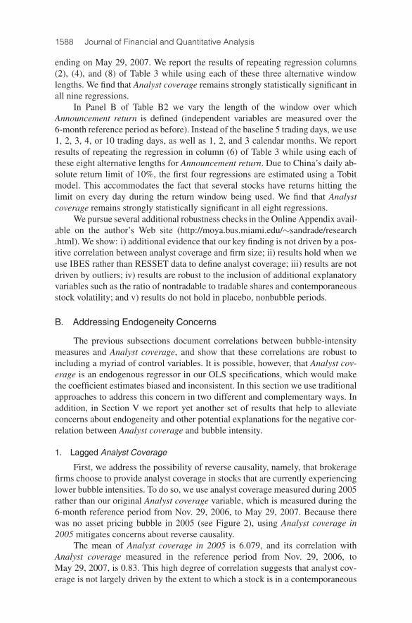
Table 5 reports the results. Column (1) shows that Analyst coverage is neg-atively related to the China-Hong Kong premium, consistent with informationdissemination reducing bubble magnitudes. Columns (2) and (3) show that thenegative association between Analyst coverage and China-HK premium is robustto the inclusion of Log of market capitalization and Daily turnover.
TABLE 5
Regressions Explaining the China-Hong Kong Premium of Dual-Listed Stocks
Table 5 reports ordinary least squares regressions that explain China-HK premium for a subsample of 23 stocks with dualtrading in Shanghai and in Hong Kong. The sample consists of 623 Shanghai A-shares, selected by requiring that sharesbe traded on at least 90% of the trading days in the reference period. The reference period is from Nov. 29, 2006, toMay 29, 2007. The variables are described in Table B1 of Appendix B. We report heteroskedasticity-robust t-statisticsin parentheses below variable coefficients. ***, **, and * denote statistical significance at the 1%, 5%, and 10% levels,respectively.
Dependent Variable: China-HK Premium
Explanatory Variables (1) (2) (3) (4) (5) (6)
Analyst coverage –6.015*** –6.182** –6.022** –3.652 –3.000 –4.709***(–4.31) (–2.71) (–2.14) (–1.06) (–0.93) (–3.24)
Log of market capitalization 0.975 3.242 –11.290 –1.962(0.11) (0.46) (–0.70) (–0.09)
Turnover –21.337 –4.300 14.091(–0.96) (–0.32) (0.21)
Lagged return volatility 2.059 1.053 0.541(1.12) (0.46) (0.24)
Lagged P/E ratio 0.682* 0.829* 0.474***(2.02) (2.15) (5.75)
Effective spread –1.682 0.615(–0.53) (0.18)
Depth 10.333 6.533(1.01) (0.51)
Market beta 69.4 109.4(0.59) (0.78)
Liquidity beta 13.780 –10.870(0.25) (–0.20)
ΔTurnover 23.125(0.24)
ΔEffective spread 5.795(0.84)
Constant 163.7*** 163.0*** 90.6 55.8 –44.165 123.6(5.55) (5.47) (0.99) (0.33) (–0.24) (3.82)
No. of obs. 23 23 23 23 23 23Adj. R2 0.45 0.43 0.44 0.50 0.46 0.58
19In addition to the small sample size concern, it is possible that inferences made with this samplemay not be representative of the entire universe of Chinese stocks because the listing of firms inHong Kong is not likely to be random. Yet another caveat is that the twin share premiums may reflectinformation asymmetry between Chinese and foreign investors, as discussed in Chan, Menkveld, andYang (2008).
1592 Journal of Financial and Quantitative Analysis
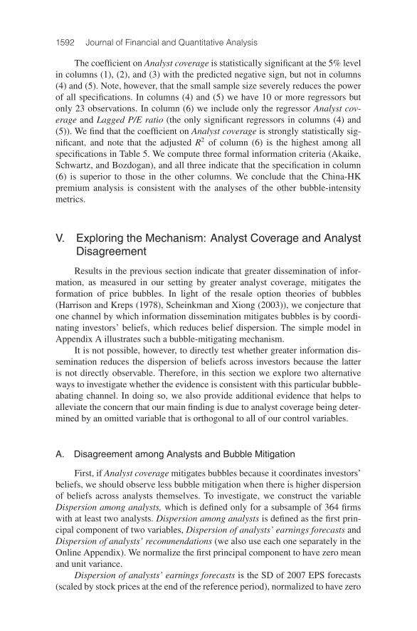
The coefficient on Analyst coverage is statistically significant at the 5% levelin columns (1), (2), and (3) with the predicted negative sign, but not in columns(4) and (5). Note, however, that the small sample size severely reduces the powerof all specifications. In columns (4) and (5) we have 10 or more regressors butonly 23 observations. In column (6) we include only the regressor Analyst cov-erage and Lagged P/E ratio (the only significant regressors in columns (4) and(5)). We find that the coefficient on Analyst coverage is strongly statistically sig-nificant, and note that the adjusted R2 of column (6) is the highest among allspecifications in Table 5. We compute three formal information criteria (Akaike,Schwartz, and Bozdogan), and all three indicate that the specification in column(6) is superior to those in the other columns. We conclude that the China-HKpremium analysis is consistent with the analyses of the other bubble-intensitymetrics.
V. Exploring the Mechanism: Analyst Coverage and AnalystDisagreement
Results in the previous section indicate that greater dissemination of infor-mation, as measured in our setting by greater analyst coverage, mitigates theformation of price bubbles. In light of the resale option theories of bubbles(Harrison and Kreps (1978), Scheinkman and Xiong (2003)), we conjecture thatone channel by which information dissemination mitigates bubbles is by coordi-nating investors’ beliefs, which reduces belief dispersion. The simple model inAppendix A illustrates such a bubble-mitigating mechanism.
It is not possible, however, to directly test whether greater information dis-semination reduces the dispersion of beliefs across investors because the latteris not directly observable. Therefore, in this section we explore two alternativeways to investigate whether the evidence is consistent with this particular bubble-abating channel. In doing so, we also provide additional evidence that helps toalleviate the concern that our main finding is due to analyst coverage being deter-mined by an omitted variable that is orthogonal to all of our control variables.
A. Disagreement among Analysts and Bubble Mitigation
First, if Analyst coverage mitigates bubbles because it coordinates investors’beliefs, we should observe less bubble mitigation when there is higher dispersionof beliefs across analysts themselves. To investigate, we construct the variableDispersion among analysts, which is defined only for a subsample of 364 firmswith at least two analysts. Dispersion among analysts is defined as the first prin-cipal component of two variables, Dispersion of analysts’ earnings forecasts andDispersion of analysts’ recommendations (we also use each one separately in theOnline Appendix). We normalize the first principal component to have zero meanand unit variance.
Dispersion of analysts’ earnings forecasts is the SD of 2007 EPS forecasts(scaled by stock prices at the end of the reference period), normalized to have zero

Andrade, Bian, and Burch 1593
mean and unit variance.20 To define Dispersion of analysts’ recommendations, wefirst map the five possible buy/sell recommendations (strong buy, buy, hold, sell,and strong sell) into one of five integer values ranging from −2 (strong sell) to+2 (strong buy). Then we compute the SD across analysts’ recommendations forthe stock using the last recommendation made by each analyst during the refer-ence period, and we normalize the variable to have zero mean and unit variance.21
Note that because both Dispersion of analysts’ earnings forecasts and Dispersionof analysts’ recommendations are normalized variables and are positively corre-lated, their first principal component is equal to their sum. Hence, one can thinkof Dispersion among analysts as the (normalized) average between Dispersionof analysts’ earnings forecasts and Dispersion of analysts’ recommendations.
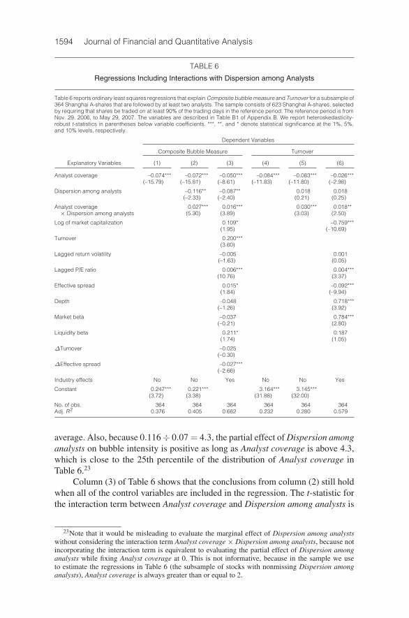
In Table 6 we regress bubble-intensity measures on Analyst coverage and theinteraction between Analyst coverage and Dispersion among analysts. A negativecoefficient on the interaction term indicates that Analyst coverage is less effec-tive in mitigating bubbles when there is a high degree of disagreement amonganalysts.
In column (1) of Table 6, we observe that the strong negative associationbetween Analyst coverage and Composite bubble measure continues to hold in aregression using the subsample of firms with at least two analysts. Column (2)shows that the coefficient on the interaction between Analyst coverage and Dis-persion among analysts is positive and statistically significant (t-statistic= 5.30),consistent with Analyst coverage having a weaker effect on bubble magnitudeswhen analysts’ beliefs are less homogenous. The effect is economically signifi-cant: The coefficient of 0.027 on the interaction term implies that a one-SD in-crease in Dispersion among analysts (which has zero mean and unity SD) reducesthe bubble-mitigating impact of Analyst coverage from 0.072 to 0.045 (whichis 0.072, the coefficient on Analyst coverage, minus the 0.027 interaction termcoefficient).
Note that Analyst coverage remains strongly statistically significant whenthe analyst dispersion variables are included in the regression, which ( jointly withthe positive signal of the interaction term) implies that the partial effect of Analystcoverage on bubble intensity is positive when Dispersion among analysts is equalto its average value of 0. Similarly, the partial effect of Dispersion among analystson bubble intensity is positive when Analyst coverage is equal to its (Table 6)average of 10.1, because −0.116 + 0.027 × 10.1 = 0.157.22 In fact, because0.072 ÷ 0.027 = 2.7, the partial effect of Analyst coverage on bubble intensityis positive as long as Dispersion among analysts is not 2.7 SDs or more below its
20For each brokerage firm-stock pair, we use the last earnings forecast made during the referenceperiod, scaled by the stock price at the date at which the forecast was made. We then normalize thedispersion variable to zero mean and unit variance. Before the normalization, Dispersion of analysts’forecasts has mean equal to 1.19%, which is on the same order of magnitude as the average earningsper price ratio, and it has an SD equal to 0.92%.
21Before the normalization, Dispersion of analysts’ recommendations has a mean of 0.70 and anSD of 0.33.
22Note that the sample in Table 6 is restricted to the stocks in which Analyst coverage is greaterthan or equal to 2. This is because it is not possible to compute a dispersion among analysts if thereare fewer than two analysts. The sample mean and sample SDs of Analyst coverage here are 10.1 and6.7, respectively, rather than the full-sample averages and SDs of 6.1 and 7.1.
1594 Journal of Financial and Quantitative Analysis
TABLE 6
Regressions Including Interactions with Dispersion among Analysts
Table 6 reports ordinary least squares regressions that explain Composite bubble measure and Turnover for a subsample of364 Shanghai A-shares that are followed by at least two analysts. The sample consists of 623 Shanghai A-shares, selectedby requiring that shares be traded on at least 90% of the trading days in the reference period. The reference period is fromNov. 29, 2006, to May 29, 2007. The variables are described in Table B1 of Appendix B. We report heteroskedasticity-robust t-statistics in parentheses below variable coefficients. ***, **, and * denote statistical significance at the 1%, 5%,and 10% levels, respectively.
Dependent Variables
Composite Bubble Measure Turnover
Explanatory Variables (1) (2) (3) (4) (5) (6)
Analyst coverage –0.074*** –0.072*** –0.050*** –0.084*** –0.083*** –0.026***(–15.79) (–15.81) (–8.61) (–11.83) (–11.80) (–2.98)
Dispersion among analysts –0.116** –0.087** 0.018 0.018(–2.33) (–2.40) (0.21) (0.25)
Analyst coverage 0.027*** 0.016*** 0.030*** 0.018**× Dispersion among analysts (5.30) (3.89) (3.03) (2.50)
Log of market capitalization 0.109* –0.759***(1.95) (–10.69)
Turnover 0.200***(3.60)
Lagged return volatility –0.005 0.001(–1.63) (0.05)
Lagged P/E ratio 0.006*** 0.004***(10.76) (3.37)
Effective spread 0.015* –0.092***(1.84) (–9.94)
Depth –0.048 0.718***(–1.26) (3.92)
Market beta –0.037 0.784***(–0.21) (2.80)
Liquidity beta 0.211* 0.187(1.74) (1.05)
ΔTurnover –0.025(–0.30)
ΔEffective spread –0.027***(–2.66)
Industry effects No No Yes No No Yes
Constant 0.247*** 0.221*** 3.164*** 3.145***(3.72) (3.38) (31.88) (32.00)
No. of obs. 364 364 364 364 364 364Adj. R2 0.376 0.405 0.682 0.232 0.280 0.579
average. Also, because 0.116÷ 0.07= 4.3, the partial effect of Dispersion amonganalysts on bubble intensity is positive as long as Analyst coverage is above 4.3,which is close to the 25th percentile of the distribution of Analyst coverage inTable 6.23
Column (3) of Table 6 shows that the conclusions from column (2) still holdwhen all of the control variables are included in the regression. The t-statistic forthe interaction term between Analyst coverage and Dispersion among analysts is
23Note that it would be misleading to evaluate the marginal effect of Dispersion among analystswithout considering the interaction term Analyst coverage× Dispersion among analysts, because notincorporating the interaction term is equivalent to evaluating the partial effect of Dispersion amonganalysts while fixing Analyst coverage at 0. This is not informative, because in the sample we useto estimate the regressions in Table 6 (the subsample of stocks with nonmissing Dispersion amonganalysts), Analyst coverage is always greater than or equal to 2.
Andrade, Bian, and Burch 1595
3.89, and the effect remains economically significant, as coefficients imply thata one-SD increase in Dispersion among analysts reduces the bubble-mitigatingeffect of Analyst coverage from 0.050 to 0.034.24
In the Online Appendix we provide a graphical illustration of the regressionresults in Table 6. There we sort stocks into six Dispersion among analysts bins,and then within each sixtile we further categorize stocks into high and low analystcoverage groups, based on whether the stock’s analyst coverage is above or belowthe overall sample median. Figure OA-2 in the Online Appendix shows that thedifference in bubble intensity among low and high Analyst coverage bins is alwayspositive but decreases mononotically as the level of disagreement among analystsincreases from sixtile 1 to sixtile 6 of Dispersion among analysts.
It is important to note that the finding that analyst coverage is less effectivein mitigating bubbles when there is more disagreement among analysts is impor-tant not only because it sheds light on the mechanism by which analyst coveragemitigates bubbles, but also because it further alleviates concerns about endogene-ity. If Analyst coverage is correlated with bubble intensity solely because bothvariables are determined by a third, stock-specific variable orthogonal to all ourcontrol variables, then how analysts disseminate the information (with more orless disagreement) would be irrelevant. The significance of the interaction termbetween Analyst coverage and analyst disagreement shows this is not the case.
B. Disagreement among Analysts and Turnover Reduction
A second way to investigate whether greater information dissemination mit-igates bubbles because it reduces the dispersion of investors’ beliefs is by usingtrading activity (i.e., turnover) as a proxy for the dispersion of investors’ beliefs.Trading activity is positively related to belief dispersion not only in Scheinkmanand Xiong’s (2003) theory of bubbles, but also in several other theories.25 Incolumns (4)–(6) of Table 6, we regress Turnover on Analyst coverage and otherexplanatory variables.
The results reported in column (4) show that, consistent with greater infor-mation dissemination reducing the dispersion of investors’ beliefs, Analyst cover-age is negatively correlated with Turnover (t-statistic = −11.83). Following thelogic of our earlier Table 6 Composite bubble measure regressions, we expect the
24The Online Appendix contains additional robustness checks. First, we report results of Com-posite bubble measure regressions interacting Analyst coverage with the individual components ofDispersion among analysts (Dispersion of analysts’ earnings forecasts and Dispersion of analysts’recommendations). Second, we show that Analyst coverage and the interaction term between Analystcoverage and dispersion remain statistically significant with the expected sign. Finally, we also reportresults of regressions using the other bubble-intensity measures (Cumulative return, Announcementreturn, and P/E ratio) rather than Composite bubble measure.
25See, for example, Shalen (1993), Hong and Stein (2003), and Cao and Ou-Yang (2009). Note,however, in the theory that motivates our work, the possibility of future disagreement that determinestoday’s bubble magnitudes, and not only the current disagreement (which is assumed away in thetheory). Therefore, realized, contemporaneous turnover may not fully capture the dispersion of beliefsthat determines bubble magnitudes. Moreover, trading activity is only a noisy proxy for the currentdispersion of beliefs. Work by Lo and Wang (2000) implies that cross-sectional differences in turnoverdo not entirely reflect cross-sectional differences in the dispersion of investors’ beliefs because otherfactors may also affect turnover. See also Cremers and Mei (2007).

1596 Journal of Financial and Quantitative Analysis
turnover-reducing effect of Analyst coverage to be weaker when there is higherdispersion of analysts’ beliefs.
Column (5) of Table 6 shows that the coefficient on the interaction term be-tween Analyst coverage and Dispersion among analysts is positive as expected,and statistically significant at the 1% level (t-statistic = 3.03). The interactioneffect is also economically significant. The 0.030 coefficient on the interactionof Analyst coverage and Dispersion among analysts implies that a one-SD in-crease of Analyst coverage decreases Turnover by only 0.30 SD when Dispersionamong analysts is one SD above its mean of 0. We also observe that Analyst cov-erage is an economically significant determinant of Turnover in column (5) onits own. Holding Dispersion among analysts constant at its mean value of 0, aone-SD increase in Analyst coverage reduces Turnover by 0.47 SD. Column (6)shows that these conclusions hold after including a myriad of control variables inthe Turnover regression. The coefficients on Analyst coverage and its interactionwith Dispersion among analysts remain significant at the 5% level (t-statistics are−2.98 and 2.50, respectively).26
The results in Table 6 provide evidence consistent with greater informationdissemination reducing bubble intensity by coordinating investors’ beliefs, whichreduces belief dispersion across investors. This is consistent with the resale optiontheories of Harrison and Kreps (1978) and Scheinkman and Xiong (2003), andwith our simple model of bubble mitigation in Appendix A.
VI. Investigating Other Plausible Mechanisms
The results in Section V suggest that one channel through which analystcoverage mitigates bubbles is by coordinating investors’ beliefs, which results inlower belief dispersion. On the basis of these results alone, however, we cannotrule out the possibility that analyst coverage also mitigates bubbles by reducinginvestors’ overoptimism. In this subsection we provide some evidence suggestingthat this alternative channel seems unlikely in our setting. In addition, we providefurther evidence against explanations in which analyst coverage only appears tomitigate bubbles because it is endogenously correlated with bubble intensities.
A. Analyst Coverage and Overoptimism
We track analyst buy/sell recommendations over time. As previously men-tioned, analysts choose one of five recommendation categories: strong buy, buy,hold, sell, and strong sell. We assign scores of +2, +1, 0, −1, and −2 to thesecategories, respectively. We first compute the mean score across analysts for eachstock and each month using only recommendations issued that month, and thenwe compute the average across stocks each month.
26Our Online Appendix contains several robustness checks. We show that the negative associationbetween Analyst coverage and Turnover also obtains in regressions with the full sample of 623 stocks,rather than just the 364 with at least two analysts. We also report results of Turnover regressions in-teracting Analyst coverage with the individual components of Dispersion among analysts (Dispersionof analysts’ earnings forecasts and Dispersion of analysts’ recommendations).

Andrade, Bian, and Burch 1597
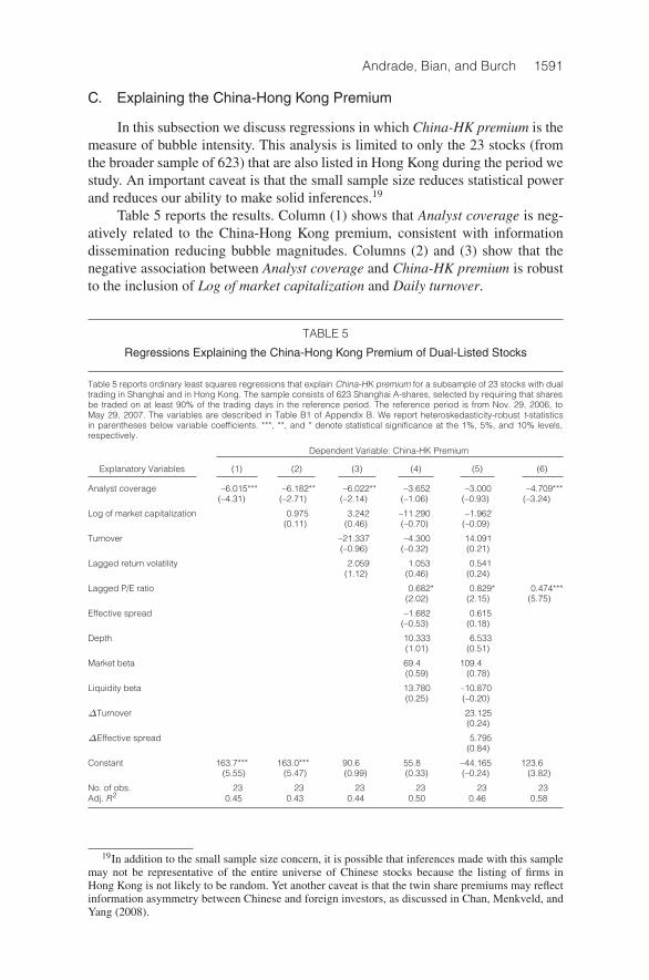
Figure 3 plots the time series of the cross-sectional average buy/sell recom-mendation. Note that the average is close to +1 from mid-2006 to early 2008, in-cluding during our entire reference period from Nov. 29, 2006, to May 30, 2007. Ifanything, the average recommendation becomes slightly more optimistic over thattime. The lack of time-series variation in the average analyst recommendation in-dicates that analysts do not become less optimistic as the bubble develops. In turn,this suggests that it is unlikely that analyst coverage mitigates bubbles in our set-ting by leaning against high valuations, thereby reducing investor overoptimism.
FIGURE 3
Average Buy/Sell Recommendation
Figure 3 illustrates the average analyst buy/sell recommendation over time. Recommendations are assigned scores 0(hold), +1 (buy), −1 (sell), +2 (strong buy), and −2 (strong sell). We first compute the mean score across analysts foreach stock and each month using only recommendations issued that month, and then we compute the average acrossstocks each month. The sample consists of 623 Shanghai A-shares.
B. Endogeneity of Analyst Coverage
Earlier in the paper we present multiple pieces of evidence that address theconcern analyst coverage may not mitigate bubbles because it is merely endoge-nously correlated with bubble intensities. Nonetheless, in this section we brieflyflesh out three specific endogeneity-based explanations and examine further evi-dence relating to them.
Lazy Analysts. It is possible that, to the extent that analyst expertise is ascarce resource in China, analysts choose to cover stocks for which forecastingearnings and issuing recommendations is easier. There could be less room for dis-agreement about these stocks, and hence they would develop smaller bubbles ac-cording to the logic of resale option theories of bubbles. However, we do not findthat analyst coverage is greater for stocks that are easier to value as measured bythe disagreement among analysts, which is a measure of “hard-to-valueness” (e.g.,Zhang (2006)). The correlation between Analyst coverage and dispersion of earn-ings forecasts is both economically and statistically insignificant (correlation =−0.03, p-value = 0.57). Moreover, the correlation between Analyst coverageand dispersion of buy/sell/recommendations is nearly statistically significant

1598 Journal of Financial and Quantitative Analysis
at the 10% level, but in the opposite direction than this explanation predicts(correlation = 0.085, p-value = 0.11).27
Moreover, in untabulated regressions we add disagreement among analystsand measures of firm age as explanatory variables in the regressions in Table 3 andfind that the coefficient on Analyst coverage remains highly economically and sta-tistically significant. Note also that the regressions in Table 3 already have indus-try fixed effects included, which controls for the possibility that some industriesare more bubble-prone (or harder to value) than others.
Overall, the evidence does not support an alternative explanation in whichthe negative correlation between Analyst coverage and bubble intensity isexplained by analysts choosing to cover stocks of firms that are older, are inmore stable or easier to value industries, or have less disagreement among an-alysts, all of which may relate to the ease of forecasting earnings and issuingrecommendations.
Institutional Sell-Off. It is possible that stocks with greater institutional own-ership before the bubble, which may attract more analyst coverage, also developsmaller bubbles because institutions influence prices downward by selling theirshares. If this were true, one would expect bubble intensities to be positively cor-related with changes in the number of stocks held by mutual funds. However, thecorrelation between our Composite bubble measure and the change in the numberof shares held by mutual funds from June 2005 to June 2007 (scaled by num-ber of tradable shares in June 2007) is economically and statistically insignificant(correlation=−0.046, p-value= 0.25). We find similarly negative, economicallysmall, and statistically insignificant correlations when we measure the change inshares from June 2006 to June 2007, or from Dec. 2006 to June 2007. Note thateven if these correlations were significant, their signs are opposite from thoseexpected. Moreover, in untabulated results the coefficient on Analyst coverage re-mains highly economically and statistically significant when we add the changein the number of shares owned by mutual funds as an explanatory variable in theregressions in Table 3. Therefore, evidence does not support the idea that stockswith larger pre-bubble institutional ownership develop smaller bubbles due to in-stitutional selling pressure.
Pump and Dump. It is possible that, when there are very few analysts, themean forecast is dominated by one or two very optimistic forecasts. These fore-casts could be strategically placed by analysts seeking to profit from a pump-and-dump strategy. Unethical analysts would choose to cover stocks that are coveredby none or a just a few other analysts, and buy shares of these stocks. Then theywould issue knowingly overoptimistic recommendations in order to inflate stockprices. At that point, they would sell shares and realize profits. We investigate thispossibility in two different ways.
First, we create a variable Analyst recommendation, equal to the mean ana-lyst recommendation in the reference period (as before, we scale analyst
27The firm’s age provides an alternative way to measure a stock’s hard-to-valueness. We find thecorrelation between Analyst coverage and the firm’s age based on date of incorporation is −0.14(p-value < 0.01), and that between Analyst coverage and the firm’s age based on date of stock-exchange listing is −0.19 ( p-value < 0.01). Both of these negative correlations refute the notion thatanalyst coverage in China is greater for firms that are easier to value.
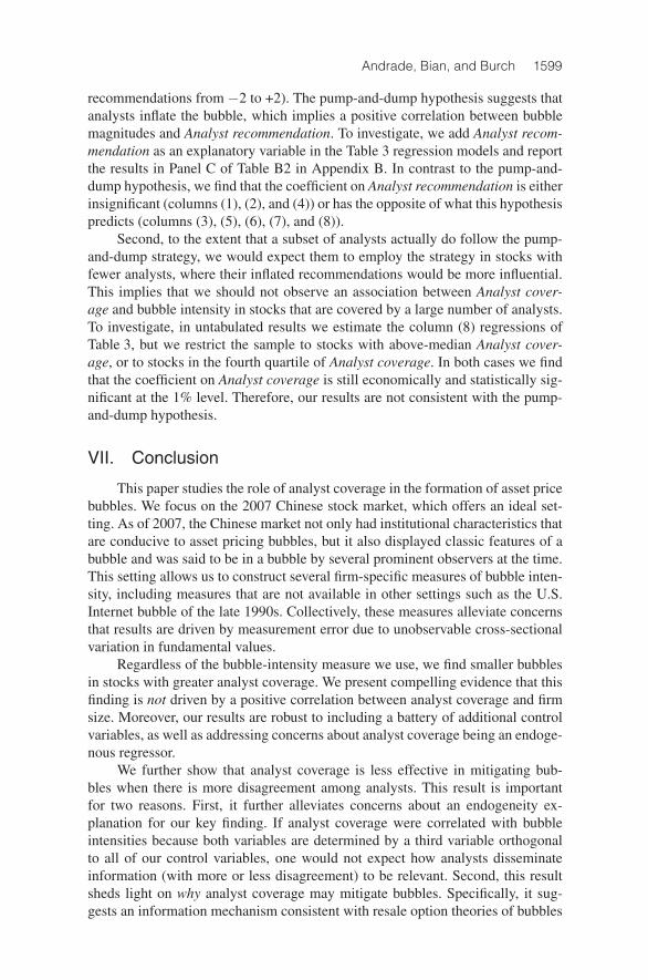
Andrade, Bian, and Burch 1599
recommendations from −2 to +2). The pump-and-dump hypothesis suggests thatanalysts inflate the bubble, which implies a positive correlation between bubblemagnitudes and Analyst recommendation. To investigate, we add Analyst recom-mendation as an explanatory variable in the Table 3 regression models and reportthe results in Panel C of Table B2 in Appendix B. In contrast to the pump-and-dump hypothesis, we find that the coefficient on Analyst recommendation is eitherinsignificant (columns (1), (2), and (4)) or has the opposite of what this hypothesispredicts (columns (3), (5), (6), (7), and (8)).
Second, to the extent that a subset of analysts actually do follow the pump-and-dump strategy, we would expect them to employ the strategy in stocks withfewer analysts, where their inflated recommendations would be more influential.This implies that we should not observe an association between Analyst cover-age and bubble intensity in stocks that are covered by a large number of analysts.To investigate, in untabulated results we estimate the column (8) regressions ofTable 3, but we restrict the sample to stocks with above-median Analyst cover-age, or to stocks in the fourth quartile of Analyst coverage. In both cases we findthat the coefficient on Analyst coverage is still economically and statistically sig-nificant at the 1% level. Therefore, our results are not consistent with the pump-and-dump hypothesis.
VII. Conclusion
This paper studies the role of analyst coverage in the formation of asset pricebubbles. We focus on the 2007 Chinese stock market, which offers an ideal set-ting. As of 2007, the Chinese market not only had institutional characteristics thatare conducive to asset pricing bubbles, but it also displayed classic features of abubble and was said to be in a bubble by several prominent observers at the time.This setting allows us to construct several firm-specific measures of bubble inten-sity, including measures that are not available in other settings such as the U.S.Internet bubble of the late 1990s. Collectively, these measures alleviate concernsthat results are driven by measurement error due to unobservable cross-sectionalvariation in fundamental values.
Regardless of the bubble-intensity measure we use, we find smaller bubblesin stocks with greater analyst coverage. We present compelling evidence that thisfinding is not driven by a positive correlation between analyst coverage and firmsize. Moreover, our results are robust to including a battery of additional controlvariables, as well as addressing concerns about analyst coverage being an endoge-nous regressor.
We further show that analyst coverage is less effective in mitigating bub-bles when there is more disagreement among analysts. This result is importantfor two reasons. First, it further alleviates concerns about an endogeneity ex-planation for our key finding. If analyst coverage were correlated with bubbleintensities because both variables are determined by a third variable orthogonalto all of our control variables, one would not expect how analysts disseminateinformation (with more or less disagreement) to be relevant. Second, this resultsheds light on why analyst coverage may mitigate bubbles. Specifically, it sug-gests an information mechanism consistent with resale option theories of bubbles

1600 Journal of Financial and Quantitative Analysis
(Harrison and Kreps (1978), Scheinkman and Xiong (2003)). That is, analystcoverage may mitigate bubbles by coordinating and thus reducing the disper-sion in investors’ beliefs, which in turn reduces the resale option component ofasset prices. In Appendix A we present a simple model illustrating this bubble-mitigation mechanism. Consistent with the mechanism, we document that stockswith greater analyst coverage display lower turnover and that, analogous to whatwe find for bubble intensities, the abating effect of analyst coverage on turnoveris weaker when there is more disagreement among analysts.
To the extent that information about asset fundamentals is a public good andthus tends to be underprovided in a laissez faire setting, our results suggest thatpolicy makers concerned with mitigating asset price bubbles should encouragepublic information dissemination. As argued by Daniel, Hirshleifer, and Teoh(2002), regulating disclosure by firms and by information intermediaries maymake asset prices more efficient providers of signals for resource allocation in aneconomy. In this regard, we note that some exchanges recognize the importanceof security analysts as disseminators of information, and that the natural provi-sion of analyst coverage by the marketplace may be suboptimal. These exchanges(e.g., Singapore, Malaysia, and London Stock Exchange’s AIM) actively sponsorthe provision of analyst coverage by subsidizing it, either directly or indirectly,and by organizing the matching of firms to analysts.
Appendix A. A Simple Model of Bubbles and AnalystCoverage
There is one risky asset, two groups of risk-neutral investors (A and B), and threedates. Investors trade at date 0 and date 1, and at date 2 the risky asset pays terminaldividend d = 1 or d = 0. The two groups of investors have common priors at date 0:the probability that d = 1 is equal to p. Therefore, if there was no trading at date 1, theequilibrium price of the risky asset at date 0 would be equal to p.
We assume, however, that at date 1 both groups of investors each observe two inde-pendent signals a and b about the asset’s payoff. The signals are equally informative:
Pr[a= 1|d = 1] = Pr[b= 1|d = 1] = q >12,
Pr[a= 0|d = 0] = Pr[b= 0|d = 0] = q >12.
Investors are assumed to be overconfident a la Scheinkman and Xiong (2003): Group Ainvestors only consider signal a (disregarding b), and similarly, group B investors onlyconsider signal b. After observing the signals, investors trade at date 1 in a market that,as in Scheinkman and Xiong, is subject to short-sale constraints. Therefore, if investorsdisagree (i.e., if signal a is different from signal b), the date 1 price only reflects the beliefsof the most optimistic investor group.
We compute equilibrium prices at date 1 under the four scenarios: (a, b) = (0, 0),(a, b)= (1, 1), (a, b)= (0, 1), and (a, b)= (1, 0). Given date 1 prices, it is straightforwardto derive the equilibrium price at date 0, which results in Proposition 1.
Proposition 1. There Is a Bubble in the Asset Price.The asset price at date 0 is
P0 = p
(1 +
(2q− 1)q(1− q)(1− p)(2q− 1)2p(1− p) + q(1− q)
)> p.(A-1)
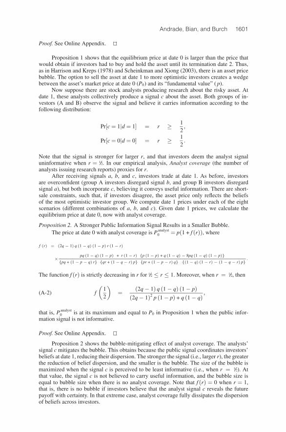
Andrade, Bian, and Burch 1601
Proof. See Online Appendix.
Proposition 1 shows that the equilibrium price at date 0 is larger than the price thatwould obtain if investors had to buy and hold the asset until its termination date 2. Thus,as in Harrison and Kreps (1978) and Scheinkman and Xiong (2003), there is an asset pricebubble. The option to sell the asset at date 1 to more optimistic investors creates a wedgebetween the asset’s market price at date 0 (P0) and its “fundamental value” ( p).
Now suppose there are stock analysts producing research about the risky asset. Atdate 1, these analysts collectively produce a signal c about the asset. Both groups of in-vestors (A and B) observe the signal and believe it carries information according to thefollowing distribution:
Pr[c= 1|d = 1] = r ≥ 12,
Pr[c= 0|d = 0] = r ≥ 12.
Note that the signal is stronger for larger r, and that investors deem the analyst signaluninformative when r = 1/2. In our empirical analysis, Analyst coverage (the number ofanalysts issuing research reports) proxies for r.
After receiving signals a, b, and c, investors trade at date 1. As before, investorsare overconfident (group A investors disregard signal b, and group B investors disregardsignal a), but both incorporate c, believing it conveys useful information. There are short-sale constraints, such that, if investors disagree, the asset price only reflects the beliefsof the most optimistic investor group. We compute date 1 prices under each of the eightscenarios (different combinations of a, b, and c). Given date 1 prices, we calculate theequilibrium price at date 0, now with analyst coverage.
Proposition 2. A Stronger Public Information Signal Results in a Smaller Bubble.The price at date 0 with analyst coverage is P analyst
0 = p(1 + f (r)), where
f (r) = (2q− 1) q (1− q) (1− p) r (1− r)
× pq (1− q) (1− p) + r (1− r) {p (1− p) + q (1− q)− 8pq (1− q) (1− p)}{pq + (1− p− q) r} {qr + (1− q− r) p} {pr + (1− p− r) q} {(1− q) (1− r)− (1− q− r) p} .
The function f (r) is strictly decreasing in r for 1/2 ≤ r ≤ 1. Moreover, when r = 1/2, then
f
(12
)=
(2q− 1) q (1− q) (1− p)
(2q− 1)2 p (1− p) + q (1− q),(A-2)
that is, P analyst0 is at its maximum and equal to P0 in Proposition 1 when the public infor-
mation signal is not informative.
Proof. See Online Appendix.
Proposition 2 shows the bubble-mitigating effect of analyst coverage. The analysts’signal c mitigates the bubble. This obtains because the public signal coordinates investors’beliefs at date 1, reducing their dispersion. The stronger the signal (i.e., larger r), the greaterthe reduction of belief dispersion, and the smaller is the bubble. The size of the bubble ismaximized when the signal c is perceived to be least informative (i.e., when r = 1/2). Atthat value, the signal c is not believed to carry useful information, and the bubble size isequal to bubble size when there is no analyst coverage. Note that f (r) = 0 when r = 1,that is, there is no bubble if investors believe that the analyst signal c reveals the futurepayoff with certainty. In that extreme case, analyst coverage fully dissipates the dispersionof beliefs across investors.

1602 Journal of Financial and Quantitative Analysis
Appendix B. Additional Tables
Table B1 describes the main variables used in the paper. Table B2 contains robustnesschecks discussed in Section IV.A.
TABLE B1
Description of Variables
Table B1 describes the main variables used in the paper. The sample consists of 623 Shanghai A-shares, selected byrequiring that shares be traded on at least 90% of the trading days in the reference period. The reference period is fromNov. 29, 2006, to May 29, 2007. All data are from RESSET.
Variable Description
Cumulative return Cumulative return during the reference period.
P/E ratio Price-earnings ratio using quarterly earnings over the most recent 12 months relative to each day’scalculation, using only public information. P/E ratio is capped at 250, and a P/E ratio equal to250 is assigned when stocks have negative earnings. Average during the reference period iscalculated from daily data.
Announcementreturn
Five-day cumulative return beginning on the day the security tax change was both announced andenacted (May 30, 2007).
Compositebubblemeasure
First principal component of Cumulative return, P/E ratio, and Announcement return, normalized tohave a mean of 0 and a variance equal to 1. It has the same orientation of Cumulative return andP/E ratio (i.e., higher Composite bubble measure is associated with larger bubbles).
China-HKpremium
Ratio of the price in China divided by the exchange-rate-adjusted price in Hong-Kong, minus 1, fora subsample of 23 dual-listed stocks. Average during the reference period is calculated fromdaily data.
Analyst coverage Number of brokerage firms issuing EPS forecasts during the reference period.
Dispersionamonganalysts
First principal component of dispersion of analyst earnings forecasts and dispersion of analystbuy/sell recommendations, normalized to have a mean of 0 and a variance equal to 1. Dispersionof earnings forecasts is the SD of 2007 EPS forecasts. For each brokerage firm-stock pair, weuse the last earnings forecast made during the reference period, scaled by the stock price at thedate at which the forecast was made. To calculate dispersion of recommendations, we first mapthe five possible buy/sell recommendations (strong buy, buy, hold, sell, and strong sell) into oneof five integer values ranging from−2 (strong sell) to +2 (strong buy). Then we compute the SDacross analysts’ recommendations for the stock using the last recommendation made by eachanalyst during the reference period. Both dispersion variables are defined for the subsample ofstocks covered by at least two analysts, and are normalized to have a mean of 0 and a varianceof 1.
Marketcapitalization
Stock price times the number of tradable shares. Average during the reference period is calculatedfrom daily data.
Turnover Number of shares traded divided by the total number of tradable shares. Average during the refer-ence period is calculated from daily data (annualized).
Lagged P/E ratio Defined as P/E ratio, but for the 6-month period immediately before the reference period.
Lagged returnvolatility
Annualized SD of average squared daily returns in the 6-month period immediately before the ref-erence period.
Effective spread Twice the difference between the transaction price and midpoint, divided by the midpoint. First wecalculate the daily average, than average daily averages across the reference period. In basispoints.
Depth One-half times the sum of the monetary quantities associated with the best bid and best ask offers.First we calculate the daily average, than average daily averages across the reference period.
Market beta Coefficient on the value-weighted market return in a regression of daily stock returns onto value-weighted market returns and an aggregate liquidity factor. The regression uses daily data duringthe reference period.
Liquidity beta Coefficient on the aggregate liquidity factor in a regression of daily stock returns onto value-weightedmarket returns and the aggregate liquidity factor. The regression uses daily data during thereference period. The aggregate liquidity factor is defined as the (daily) innovation on the averageeffective spread across all sample stocks.
ΔTurnover Average daily turnover in the 6-month period immediately after the reference period minus the av-erage daily turnover in the reference period (annualized).
ΔEffectivespread
Average in the 6-month period immediately after the reference period minus the averages in thereference period.
Industry effects Dummy variables based on 13 industries defined by the China Securities Regulatory Commission(CSRC).

Andrade, Bian, and Burch 1603
TABLE B2
Using Different Time Windows and Adding Analyst Recommendations
Panel A of Table B2 reports regressions in which variables are defined over 3-, 9-, and 12-month windows ending in May 29,2007, as opposed to the 6-month window of our baseline results in Table 6. Panel B reports regressions of Announcementreturn calculated over windows consisting of 1, 2, 3, 4, and 10 trading days, as well as 1, 2, and 3 calendar monthsfollowing the May 30, 2007, tax increase announcement, as opposed to the 5-trading day window of our baseline resultsin Table 3. We use Tobit regressions for short windows (4 days or less), and OLS regressions for longer windows. PanelC reports regressions in which Analyst recommendation is added to Table 3 regressions. Analyst recommendation is theaverage buy/sell analyst recommendation in the reference period (0 is hold, +1 buy, +2 strong buy, −1 sell, −2 strongsell). The regressions include, but we do not report below, all of the other explanatory variables included in Table 3. Thevariables are described in Table B1 of Appendix B. We report heteroskedasticity-robust t-statistics in parentheses belowvariable coefficients. ***, **, and * denote statistical significance at the 1%, 5%, and 10% levels, respectively.
Panel A. Redefine Window Lengths for Cumulative Return, P/E Ratio, Composite Bubble Measure, and ExplanatoryVariables
Dependent Variable
3 Months 9 Months 12 Months
Comp. Comp. Comp.Cum. P/E Bubble Cum. P/E Bubble Cum. P/E Bubble
Return Ratio Meas. Return Ratio Meas. Return Ratio Meas.
Analyst coverage –3.124*** –2.043*** –0.076*** –2.377*** –0.974*** –0.047*** –1.179 –1.642*** –0.043***(–6.65) (–4.92) (–11.33) (–3.34) (–3.23) (–10.11) (–1.15) (–4.34) (–8.81)
Other expl. var. in Tab. 3 Yes Yes Yes Yes Yes Yes Yes Yes Yes
No. of obs. 623 623 623 617 617 617 612 612 612Adj. R2 0.473 0.821 0.736 0.392 0.765 0.720 0.371 0.633 0.697
Panel B. Define Announcement Return Using Different Windows
Dependent Variable: Announcement Return
Announcement Return Window
1 Day 2 Days 3 Days 4 Days 10 Days 1 Month 2 Months 3 Months
Analyst coverage 0.421*** 0.515*** 0.717*** 0.740*** 0.944*** 1.143*** 1.007*** 1.315***(4.46) (6.96) (8.10) (8.82) (7.71) (8.35) (6.43) (5.90)
Other expl. var. in Tab. 3 Yes Yes Yes Yes Yes Yes Yes Yes
No. of obs. 623 623 623 623 623 623 623 623
Lower limit (censoring) –10.0% –19.0% –27.1% –34.4% — — — —
Censored observations 449 132 122 109 — — — —
Adj. R2 — — — — 0.45 0.46 0.38 0.36
Panel C. Add Analyst Recommendation
Dependent Variable
Cumulative P/E Announcement CompositeReturn Ratio Return Bubble Measure
(1) (2) (3) (4) (5) (6) (7) (8)
Analyst coverage –4.911*** –4.760*** –3.217*** –0.489** 0.846*** 0.573*** –0.077*** –0.049***(–10.85) (–6.84) (–8.99) (–2.01) (14.57) (6.76) (–18.08) (–9.17)
Analyst recommendation –1.691 1.506 –19.323*** –4.863 3.182*** 2.677*** –0.257*** –0.139***(–0.25) (0.27) (–3.09) (–1.47) (5.36) (4.35) (–4.23) (–2.97)
Other expl. var. in Tab. 3 No Yes No Yes No Yes No Yes
No. of obs. 450 450 450 450 450 450 450 450Adj. R2 0.166 0.465 0.187 0.846 0.432 0.526 0.467 0.714
ReferencesAcharya, V., and L. Pedersen. “Asset Pricing with Liquidity Risk.” Journal of Financial Economics,
77 (2005), 375–410.Allen, F. “What Is Systemic Risk and How Should We Deal with It?” Speech at the 11th Meeting of
the Brazilian Finance Society (2011).
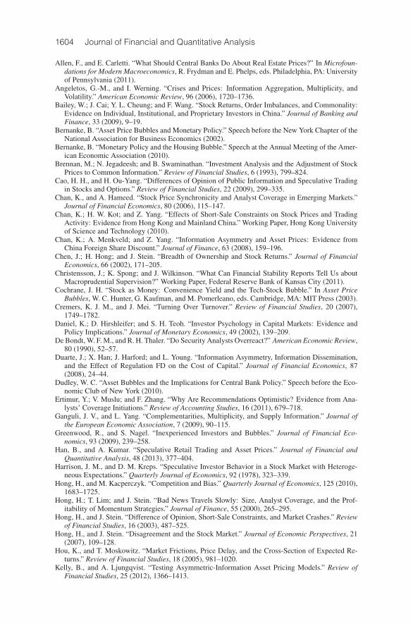
1604 Journal of Financial and Quantitative Analysis
Allen, F., and E. Carletti. “What Should Central Banks Do About Real Estate Prices?” In Microfoun-dations for Modern Macroeconomics, R. Frydman and E. Phelps, eds. Philadelphia, PA: Universityof Pennsylvania (2011).
Angeletos, G.-M., and I. Werning. “Crises and Prices: Information Aggregation, Multiplicity, andVolatility.” American Economic Review, 96 (2006), 1720–1736.
Bailey, W.; J. Cai; Y. L. Cheung; and F. Wang. “Stock Returns, Order Imbalances, and Commonality:Evidence on Individual, Institutional, and Proprietary Investors in China.” Journal of Banking andFinance, 33 (2009), 9–19.
Bernanke, B. “Asset Price Bubbles and Monetary Policy.” Speech before the New York Chapter of theNational Association for Business Economics (2002).
Bernanke, B. “Monetary Policy and the Housing Bubble.” Speech at the Annual Meeting of the Amer-ican Economic Association (2010).
Brennan, M.; N. Jegadeesh; and B. Swaminathan. “Investment Analysis and the Adjustment of StockPrices to Common Information.” Review of Financial Studies, 6 (1993), 799–824.
Cao, H. H., and H. Ou-Yang. “Differences of Opinion of Public Information and Speculative Tradingin Stocks and Options.” Review of Financial Studies, 22 (2009), 299–335.
Chan, K., and A. Hameed. “Stock Price Synchronicity and Analyst Coverage in Emerging Markets.”Journal of Financial Economics, 80 (2006), 115–147.
Chan, K.; H. W. Kot; and Z. Yang. “Effects of Short-Sale Constraints on Stock Prices and TradingActivity: Evidence from Hong Kong and Mainland China.” Working Paper, Hong Kong Universityof Science and Technology (2010).
Chan, K.; A. Menkveld; and Z. Yang. “Information Asymmetry and Asset Prices: Evidence fromChina Foreign Share Discount.” Journal of Finance, 63 (2008), 159–196.
Chen, J.; H. Hong; and J. Stein. “Breadth of Ownership and Stock Returns.” Journal of FinancialEconomics, 66 (2002), 171–205.
Christensson, J.; K. Spong; and J. Wilkinson. “What Can Financial Stability Reports Tell Us aboutMacroprudential Supervision?” Working Paper, Federal Reserve Bank of Kansas City (2011).
Cochrane, J. H. “Stock as Money: Convenience Yield and the Tech-Stock Bubble.” In Asset PriceBubbles, W. C. Hunter, G. Kaufman, and M. Pomerleano, eds. Cambridge, MA: MIT Press (2003).
Cremers, K. J. M., and J. Mei. “Turning Over Turnover.” Review of Financial Studies, 20 (2007),1749–1782.
Daniel, K.; D. Hirshleifer; and S. H. Teoh. “Investor Psychology in Capital Markets: Evidence andPolicy Implications.” Journal of Monetary Economics, 49 (2002), 139–209.
De Bondt, W. F. M., and R. H. Thaler. “Do Security Analysts Overreact?” American Economic Review,80 (1990), 52–57.
Duarte, J.; X. Han; J. Harford; and L. Young. “Information Asymmetry, Information Dissemination,and the Effect of Regulation FD on the Cost of Capital.” Journal of Financial Economics, 87(2008), 24–44.
Dudley, W. C. “Asset Bubbles and the Implications for Central Bank Policy.” Speech before the Eco-nomic Club of New York (2010).
Ertimur, Y.; V. Muslu; and F. Zhang. “Why Are Recommendations Optimistic? Evidence from Ana-lysts’ Coverage Initiations.” Review of Accounting Studies, 16 (2011), 679–718.
Ganguli, J. V., and L. Yang. “Complementarities, Multiplicity, and Supply Information.” Journal ofthe European Economic Association, 7 (2009), 90–115.
Greenwood, R., and S. Nagel. “Inexperienced Investors and Bubbles.” Journal of Financial Eco-nomics, 93 (2009), 239–258.
Han, B., and A. Kumar. “Speculative Retail Trading and Asset Prices.” Journal of Financial andQuantitative Analysis, 48 (2013), 377–404.
Harrison, J. M., and D. M. Kreps. “Speculative Investor Behavior in a Stock Market with Heteroge-neous Expectations.” Quarterly Journal of Economics, 92 (1978), 323–339.
Hong, H., and M. Kacperczyk. “Competition and Bias.” Quarterly Journal of Economics, 125 (2010),1683–1725.
Hong, H.; T. Lim; and J. Stein. “Bad News Travels Slowly: Size, Analyst Coverage, and the Prof-itability of Momentum Strategies.” Journal of Finance, 55 (2000), 265–295.
Hong, H., and J. Stein. “Difference of Opinion, Short-Sale Constraints, and Market Crashes.” Reviewof Financial Studies, 16 (2003), 487–525.
Hong, H., and J. Stein. “Disagreement and the Stock Market.” Journal of Economic Perspectives, 21(2007), 109–128.
Hou, K., and T. Moskowitz. “Market Frictions, Price Delay, and the Cross-Section of Expected Re-turns.” Review of Financial Studies, 18 (2005), 981–1020.
Kelly, B., and A. Ljungqvist. “Testing Asymmetric-Information Asset Pricing Models.” Review ofFinancial Studies, 25 (2012), 1366–1413.

Andrade, Bian, and Burch 1605
Kindleberger, C., and R. Aliber. Manias, Panics, and Crashes: A History of Financial Crises, 5th ed.Hoboken, NJ: John Wiley and Sons (2005).
Kumar, A. “Hard-to-Value Stocks, Behavioral Biases, and Informed Trading.” Journal of Financialand Quantitative Analysis, 44 (2009), 1375–1401.
Landau, J.-P. “Bubbles and Macro-Prudential Regulation.” Speech at the “The Future of FinancialRegulation” conference of the Bank of France and the Toulouse School of Economics (2009).
Liu, C., and M. Seasholes. “Dual-Listed Shares and Trading.” Working Paper, Hong Kong Universityof Science and Technology (2011).
Lo, A.; H. Mamaysky; and J. Wang. “Asset Prices and Trading Volume under Fixed TransactionCosts.” Journal of Political Economy, 112 (2004), 1054–1090.
Lo, A., and J. Wang. “Trading Volume: Definitions, Data Analysis, and Implications of PortfolioTheory.” Review of Financial Studies, 13 (2000), 257–300.
Mei, J.; J. A. Scheinkman; and W. Xiong. “Speculative Trading and Stock Prices: Evidence fromChinese A-B Share Premia.” Annals of Economics and Finance, 10 (2009), 225–255.
Miller, E. M. “Risk, Uncertainty, and Divergence of Opinion.” Journal of Finance, 32 (1977),1151–1168.
Moshirian, F.; D. Ng; and E. Wu. “The Value of Stock Analysts’ Recommendations: Evidence fromEmerging Markets.” International Review of Financial Analysis, 18 (2009), 74–83.
Prasad, E. “After the Fall.” Finance and Development, 47 (2010), 22–25.Ross, S. “The Arbitrage Theory of Capital Asset Pricing.” Journal of Economic Theory, 13 (1976),
341–360.Scheinkman, J. A., and W. Xiong. “Overconfidence and Speculative Bubbles.” Journal of Political
Economy, 111 (2003), 1183–1219.Shalen, C. T. “Volume, Volatility, and Dispersion of Beliefs.” Review of Financial Studies, 6 (1993),
405–434.Shiller, R. J. Irrational Exuberance, 2nd ed. Princeton, NJ: Princeton University Press (2005).Xiong, W., and J. Yu. “The Chinese Warrants Bubble.” American Economic Review, 101 (2011),
2723–2753.Zhang, X. F. “Information Uncertainty and Stock Returns.” Journal of Finance, 61 (2006), 105–136.