Analysis of variance

Analysis of variance

Tron Anders Moger2006.31.10

Comparing more than two groups

• Up to now we have studied situations with– One observation per object

• One group• Two groups

– Two or more observations per object• We will now study situations with one observation

per object, and three or more groups of objects• The most important question is as usual: Do the

numbers in the groups come from the same population, or from different populations?

ANOVA

• If you have three groups, could plausibly do pairwise comparisons. But if you have 10 groups? Too many pairwise comparisons: You would get too many false positives!

• You would really like to compare a null hypothesis of all equal, against some difference

• ANOVA: ANalysis Of VAriance

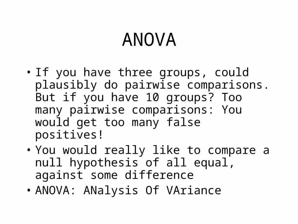
One-way ANOVA: Example• Assume ”treatment results” from 13 patients

visiting one of three doctors are given: – Doctor A: 24,26,31,27– Doctor B: 29,31,30,36,33– Doctor C: 29,27,34,26

• H0: The means are equal for all groups (The treatment results are from the same population of results)

• H1: The means are different for at least two groups (They are from different populations)

Comparing the groups

• Averages within groups: – Doctor A: 27– Doctor B: 31.8– Doctor C: 29

• Total average: • Variance around the mean matters for comparison. • We must compare the variance within the groups

to the variance between the group means.

4 27 5 31.8 4 29 29.464 5 4

Variance within and between groups

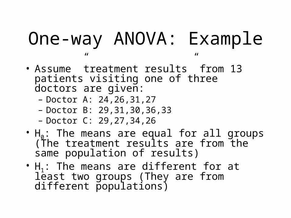
• Sum of squares within groups:

• Compare it with sum of squares between groups:

• Comparing these, we also need to take into account the number of observations and sizes of groups

2 2 2(24 27) (26 27) ... (29 31.8) .... 94.8SSW

2 2 2

2 2 2

(27 29.46) (27 29.46) ... (31.8 29.46) ....

4(27 29.46) 5(31.8 29.46) 4(29 29.46) 52.43

SSG

2

1 1

( )inK

ij ii j

SSW x x

2

1

( )K

i ii

SSG n x x

Adjusting for group sizes

• Divide by the number of degrees of freedom

• Test statistic: reject H0 if this is large

SSWMSWn K

1SSGMSGK

MSGMSW

Both are estimates of population variance of error under H0

n: number of observationsK: number of groups

Test statistic thresholds• If populations are normal, with the same

variance, then we can show that under the null hypothesis, MSG and MSW are Chi-square distributed with K-1 and n-K d.f.

• Reject at confidence level if

1,~ K n KMSG FMSW

1, ,K n KMSG FMSW

The F distribution, with K-1 and n-K degrees of freedom

Find this value in table p. 871

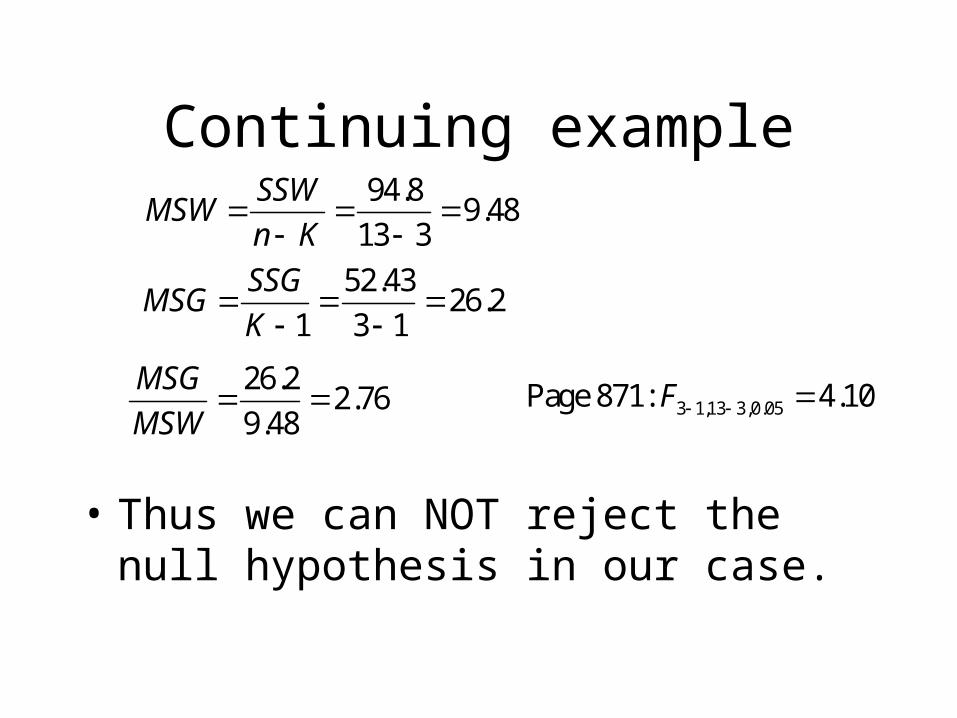
Continuing example

• Thus we can NOT reject the null hypothesis in our case.

94.8 9.4813 3

SSWMSWn K

52.43 26.21 3 1

SSGMSGK

26.2 2.769.48

MSGMSW

3 1,13 3,0.05Page 871: 4.10F

ANOVA table

Source of variation

Sum of squares

Deg. of freedom

Mean squares

F ratio

Between groups

SSG K-1 MSG

Within groups

SSW n-K MSW

Total SST n-1

MSGMSW

2 2 2(24 29.46) (26 29.46) ... (26 29.46)SST

SSG SSW SST NOTE:

Formulation of the model:• H0: µ1=µ2=…=µK

• Xij=µi+εij

• Let Gi be the difference between the group means and the population mean. Then:

• Gi=µi-µ of µi=µ+Gi

• Giving Xij=µ+Gi+εij

• And H0: G1=G2=…=GK=0

One-way ANOVA in SPSS

• ANOVA

VAR00001

52,431 2 26,215 2,765 ,11194,800 10 9,480

147,231 12

Between GroupsWithin GroupsTotal

Sum ofSquares df Mean Square F Sig.

Last column: The p-value: The smallest value of at which the null hypothesis is rejected.

One-way ANOVA in SPSS:

• Analyze - Compare Means - One-way ANOVA

• Move dependent variable to Dependent list and group to Factor

• Choose Bonferroni in the Post Hoc window to get comparisons of all groups

• Choose Descriptive and Homogeneity of variance test in the Options window

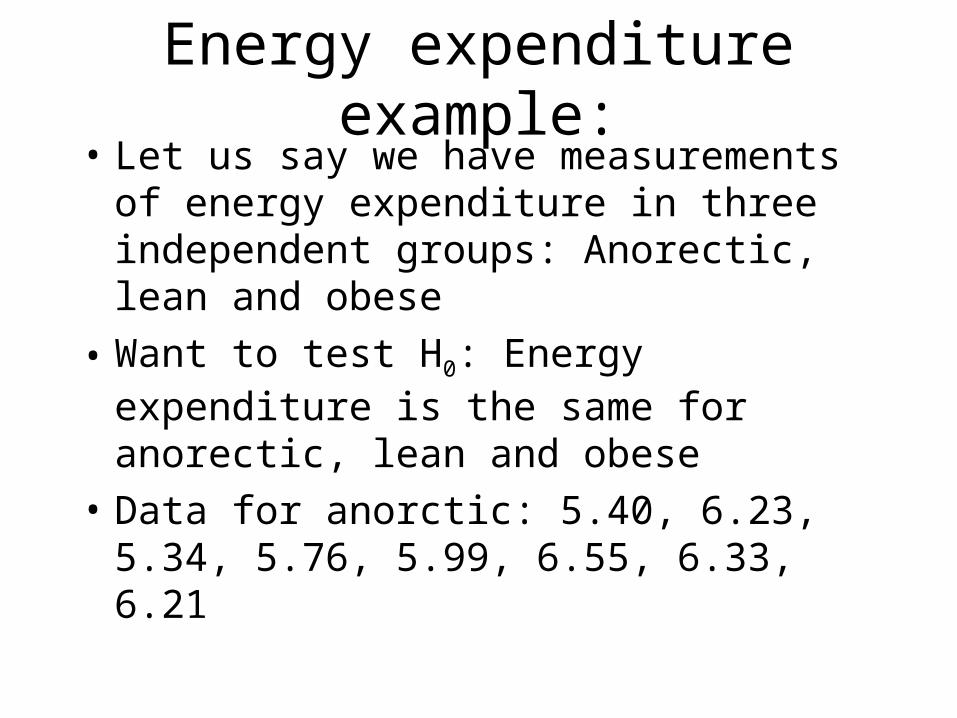
Energy expenditure example:• Let us say we have measurements of energy

expenditure in three independent groups: Anorectic, lean and obese

• Want to test H0: Energy expenditure is the same for anorectic, lean and obese

• Data for anorctic: 5.40, 6.23, 5.34, 5.76, 5.99, 6.55, 6.33, 6.21

SPSS output:

• See that there is a difference between groups.

• See also between which groups the difference is!

Descriptives

Energy

13 8,0662 1,23808 ,34338 7,3180 8,8143 6,13 10,889 10,2978 1,39787 ,46596 9,2233 11,3723 8,79 12,798 5,9762 ,44032 ,15568 5,6081 6,3444 5,34 6,55

30 8,1783 1,98936 ,36321 7,4355 8,9212 5,34 12,79

LeanObeseAnorecticTotal

N Mean Std. Deviation Std. Error Lower Bound Upper Bound

95% Confidence Interval forMean

Minimum Maximum

Test of Homogeneity of Variances

Energy

2,814 2 27 ,078

LeveneStatistic df1 df2 Sig.

ANOVA

Energy

79,385 2 39,693 30,288 ,00035,384 27 1,311

114,769 29

Between GroupsWithin GroupsTotal

Sum ofSquares df Mean Square F Sig.

Multiple Comparisons

Dependent Variable: EnergyBonferroni

-2,23162* ,49641 ,000 -3,4987 -,96462,08990* ,51441 ,001 ,7769 3,40292,23162* ,49641 ,000 ,9646 3,49874,32153* ,55626 ,000 2,9017 5,7414

-2,08990* ,51441 ,001 -3,4029 -,7769-4,32153* ,55626 ,000 -5,7414 -2,9017

(J) GroupObeseAnorecticLeanAnorecticLeanObese

(I) GroupLean

Obese

Anorectic

MeanDifference

(I-J) Std. Error Sig. Lower Bound Upper Bound95% Confidence Interval

The mean difference is significant at the .05 level.*.

Conclusion:

• There is a significant overall difference in energy expenditure between the three groups (p-value<0.001)

• There are also significant differences for all two-by-two comparisons of groups

The Kruskal-Wallis test

• ANOVA is based on the assumption of normality

• There is a non-parametric alternative not relying this assumption:– Looking at all observations together, rank them– Let R1, R2, …,RK be the sums of ranks of each

group– If some R’s are much larger than others, it

indicates the numbers in different groups come from different populations

The Kruskal-Wallis test

• The test statistic is

• Under the null hypothesis, this has an approximate distribution.

• The approximation is OK when each group contains at least 5 observations.

21K

2

1

12 3( 1)( 1)

Ki

i i

RW nn n n

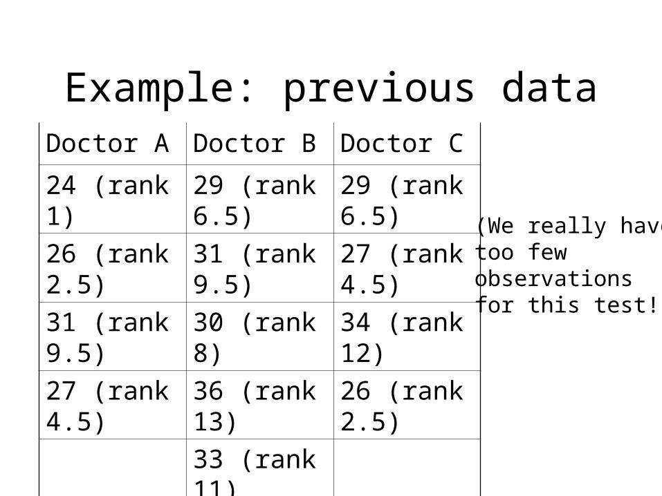
Example: previous dataDoctor A Doctor B Doctor C

24 (rank 1) 29 (rank 6.5) 29 (rank 6.5)

26 (rank 2.5) 31 (rank 9.5) 27 (rank 4.5)

31 (rank 9.5) 30 (rank 8) 34 (rank 12)

27 (rank 4.5) 36 (rank 13) 26 (rank 2.5)

33 (rank 11)

R1=17.5 R2=48 R3=25.5

(We really havetoo few observations for this test!)

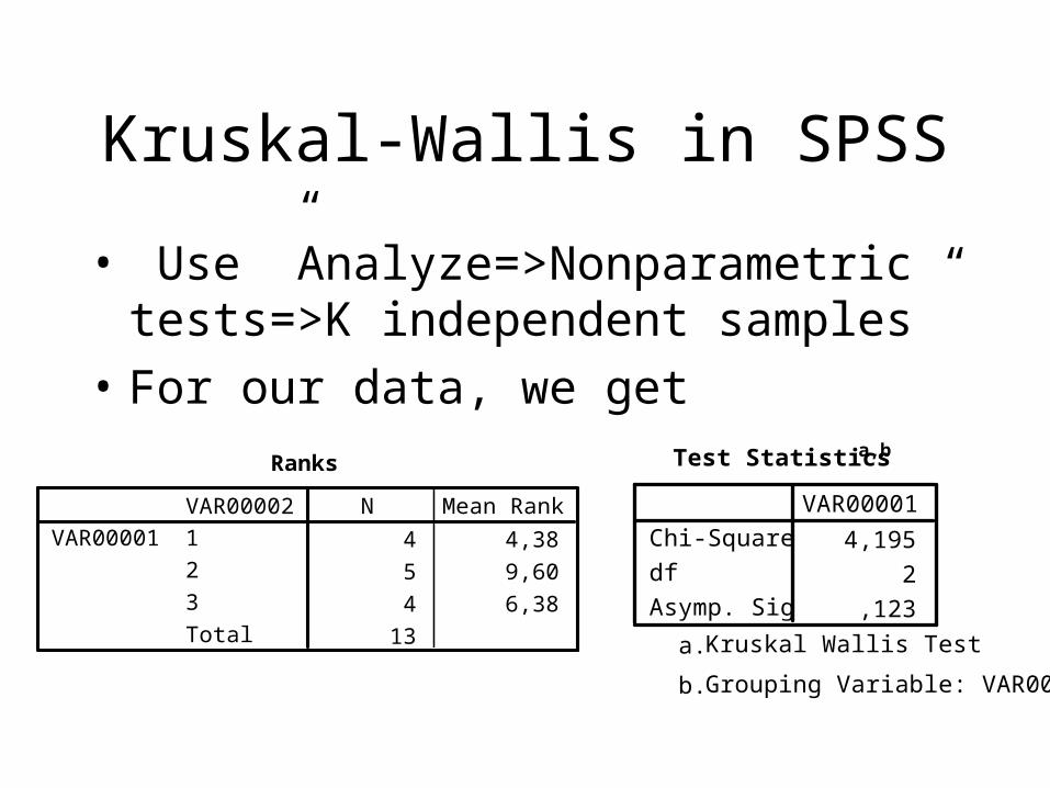
Kruskal-Wallis in SPSS

• Use ”Analyze=>Nonparametric tests=>K independent samples”

• For our data, we get Ranks

4 4,385 9,604 6,38

13

VAR00002123Total

VAR00001N Mean Rank

Test Statisticsa,b

4,1952

,123

Chi-SquaredfAsymp. Sig.

VAR00001

Kruskal Wallis Testa.

Grouping Variable: VAR00002b.

For the energy data:

• Same result as for one-way ANOVA!

• Reject H0

Ranks

13 15,629 24,678 5,00

30

GroupLeanObeseAnorecticTotal

EnergyN Mean Rank

Test Statisticsa,b

21,1462

,000

Chi-SquaredfAsymp. Sig.

Energy

Kruskal Wallis Testa.

Grouping Variable: Groupb.

When to use what method

• In situations where we have one observation per object, and want to compare two or more groups: – Use non-parametric tests if you have enough data

• For two groups: Mann-Whitney U-test (Wilcoxon rank sum)• For three or more groups use Kruskal-Wallis

– If data analysis indicate assumption of normally distributed independent errors is OK

• For two groups use t-test (equal or unequal variances assumed)• For three or more groups use ANOVA

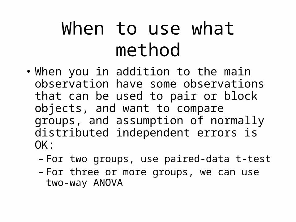
When to use what method

• When you in addition to the main observation have some observations that can be used to pair or block objects, and want to compare groups, and assumption of normally distributed independent errors is OK: – For two groups, use paired-data t-test– For three or more groups, we can use two-way

ANOVA

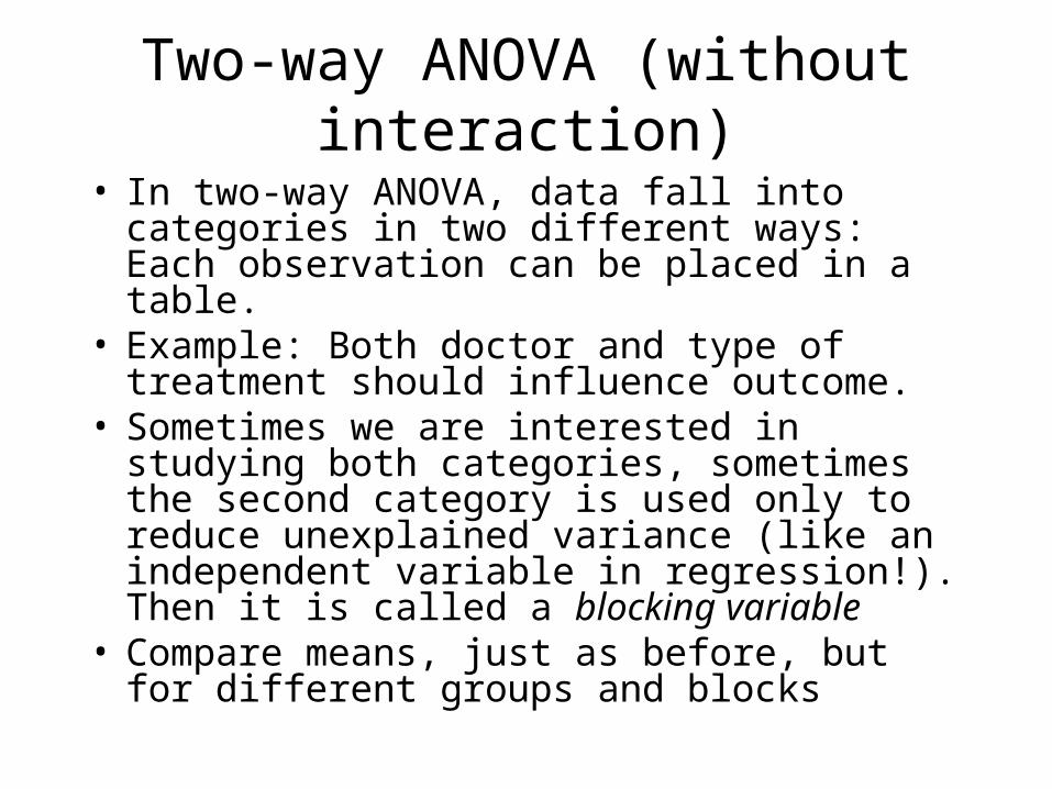
Two-way ANOVA (without interaction)

• In two-way ANOVA, data fall into categories in two different ways: Each observation can be placed in a table.

• Example: Both doctor and type of treatment should influence outcome.

• Sometimes we are interested in studying both categories, sometimes the second category is used only to reduce unexplained variance (like an independent variable in regression!). Then it is called a blocking variable

• Compare means, just as before, but for different groups and blocks

Data from exercise 17.46:• Three types of aptitude tests (K=3) given to

prospective management trainers• Each test type is given to members of each

of four groups of subjects (H=4): Profile fit, Mindbender, Psych Out

Test typeSubject type Profile fit Mindbender Psych Out

Poor 65 69 75Fair 74 72 70

Good 64 68 78Excellent 83 78 76

Sums of squares for two-way ANOVA

• Assume K groups, H blocks, and assume one observation xij for each group i and each block j, so we have n=KH observations (independent!). – Mean for category i: – Mean for block j: – Overall mean:

• Model: Xij=µ+Gi+Bj+εij

ix

jx

x

Sums of squares for two-way ANOVA

2

1

( )K

ii

SSG H x x

2

1

( )H

jj

SSB K x x

2

1 1

( )K H

ij i ji j

SSE x x x x

2

1 1

( )K H

iji j

SST x x

SSG SSB SSE SST

ANOVA table for two-way dataSource of variation

Sums of squares

Deg. of freedom

Mean squares F ratio

Between groups SSG K-1 MSG= SSG/(K-1) MSG/MSE

Between blocks SSB H-1 MSB= SSB/(H-1) MSB/MSE

Error SSE (K-1)(H-1) MSE= SSE/(K-1)(H-1)

Total SST n-1

Test for between groups effect: compare to

Test for between blocks effect: compare to

MSGMSEMSBMSE

1,( 1)( 1)K K HF

1,( 1)( 1)H K HF

Two-way ANOVA (with interaction)• The setup above assumes that the blocking

variable influences outcomes in the same way in all categories (and vice versa)

• We can check if there is interaction between the blocking variable and the categories by extending the model with an interaction term

• Need more observations per block• Other advantages: More precise estimates

Data from exercise 17.46 cont’d:• Each type of test was given three times for

each type of subject

Test typeSubject type Profile fit Mindbender Psych Out

Poor 65 68 62 69 71 67 75 75 78Fair 74 79 76 72 69 69 70 69 65

Good 64 72 65 68 73 75 78 82 80Excellent 83 82 84 78 78 75 76 77 75

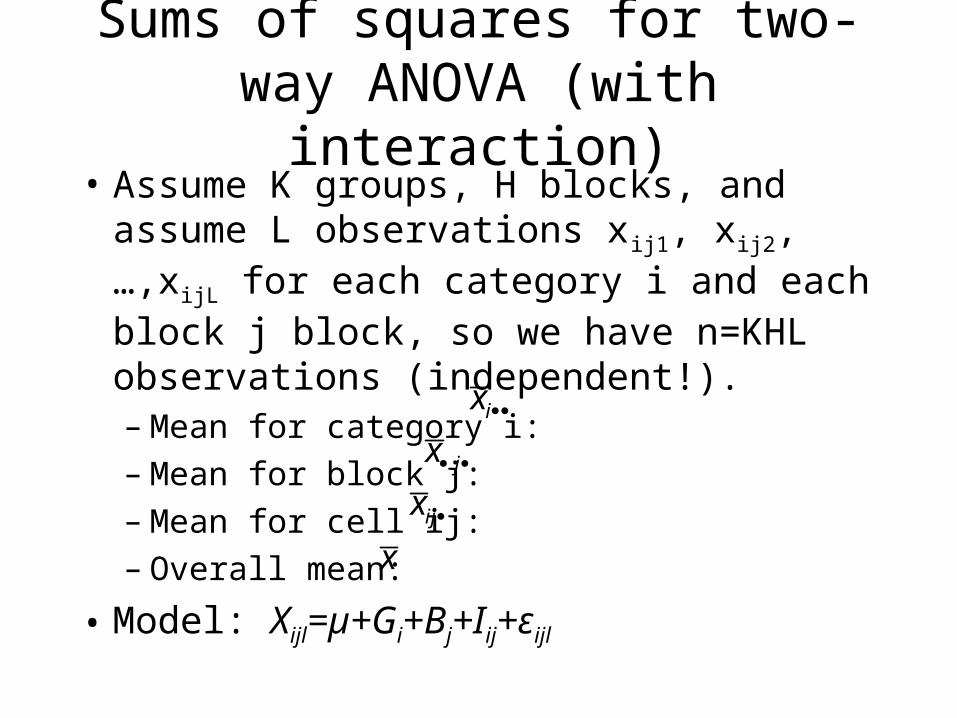
Sums of squares for two-way ANOVA (with interaction)

• Assume K groups, H blocks, and assume L observations xij1, xij2, …,xijL for each category i and each block j block, so we have n=KHL observations (independent!). – Mean for category i: – Mean for block j:– Mean for cell ij: – Overall mean:

• Model: Xijl=µ+Gi+Bj+Iij+εijl

ix

jx

xijx

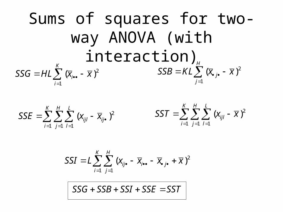
Sums of squares for two-way ANOVA (with interaction)

2

1

( )K

ii

SSG HL x x

2

1

( )H

jj

SSB KL x x

2

1 1

( )K H

ij i ji j

SSI L x x x x

2

1 1 1

( )K H L

ijli j l

SST x x

SSG SSB SSI SSE SST

2

1 1 1

( )K H L

ijl iji j l

SSE x x

ANOVA table for two-way data (with interaction)

Source of variation

Sums of squares

Deg. of freedom

Mean squares F ratio

Between groups SSG K-1 MSG= SSG/(K-1) MSG/MSE

Between blocks SSB H-1 MSB= SSB/(H-1) MSB/MSE

Interaction SSI (K-1)(H-1) MSI= SSI/(K-1)(H-1)

MSI/MSE

Error SSE KH(L-1) MSE= SSE/KH(L-1)

Total SST n-1

Test for interaction: compare MSI/MSE with

Test for block effect: compare MSB/MSE with

Test for group effect: compare MSG/MSE with 1, ( 1)K KH LF

1, ( 1)H KH LF

( 1)( 1), ( 1)K H KH LF

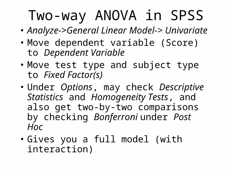
Two-way ANOVA in SPSS• Analyze->General Linear Model->

Univariate• Move dependent variable (Score) to

Dependent Variable• Move test type and subject type to Fixed

Factor(s)• Under Options, may check Descriptive

Statistics and Homogeneity Tests, and also get two-by-two comparisons by checking Bonferroni under Post Hoc

• Gives you a full model (with interaction)

Some SPSS output:• See that there is a

significant block effect, significant group effect, and a significant interaction effect

• Means (in plain words) that test score is different for subject types, for the three tests, and that difference for test type depends on what block you consider

Levene's Test of Equality of Error Variancesa

Dependent Variable: Score

1,472 11 24 ,206F df1 df2 Sig.

Tests the null hypothesis that the error variance of thedependent variable is equal across groups.

Design: Intercept+Subjectty+Testtype+Subjectty* Testtype

a.

Tests of Between-Subjects Effects


1032,556a 11 93,869 15,360 ,000193306,778 1 193306,778 31632,018 ,000

389,000 3 129,667 21,218 ,00057,556 2 28,778 4,709 ,019

586,000 6 97,667 15,982 ,000146,667 24 6,111

194486,000 361179,222 35

SourceCorrected ModelInterceptSubjecttyTesttypeSubjectty * TesttypeErrorTotalCorrected Total

Type IV Sumof Squares df Mean Square F Sig.

R Squared = ,876 (Adjusted R Squared = ,819)a.

Equal variancescan be assumed

2. Subjectty


70,000 ,824 68,299 71,70171,444 ,824 69,744 73,14573,000 ,824 71,299 74,70178,667 ,824 76,966 80,367

SubjecttyPoorFairGoodExcellent

Mean Std. Error Lower Bound Upper Bound95% Confidence Interval

Two-by-two comparisonsMultiple Comparisons

Dependent Variable: ScoreBonferroni

,83 1,009 1,000 -1,76 3,43-2,17 1,009 ,126 -4,76 ,43-,83 1,009 1,000 -3,43 1,76

-3,00* 1,009 ,020 -5,60 -,402,17 1,009 ,126 -,43 4,763,00* 1,009 ,020 ,40 5,60

(J) TesttypeMindbenderPsych OutProfile fitPsych OutProfile fitMindbender

(I) TesttypeProfile fit

Mindbender

Psych Out

MeanDifference


Based on observed means.The mean difference is significant at the ,05 level.*.

Multiple Comparisons

Dependent Variable: ScoreBonferroni

-1,44 1,165 1,000 -4,79 1,91-3,00 1,165 ,100 -6,35 ,35-8,67* 1,165 ,000 -12,02 -5,321,44 1,165 1,000 -1,91 4,79

-1,56 1,165 1,000 -4,91 1,79-7,22* 1,165 ,000 -10,57 -3,873,00 1,165 ,100 -,35 6,351,56 1,165 1,000 -1,79 4,91

-5,67* 1,165 ,000 -9,02 -2,328,67* 1,165 ,000 5,32 12,027,22* 1,165 ,000 3,87 10,575,67* 1,165 ,000 2,32 9,02

(J) SubjecttyFairGoodExcellentPoorGoodExcellentPoorFairExcellentPoorFairGood

(I) SubjecttyPoor

Fair

Good

Excellent

MeanDifference


Based on observed means.The mean difference is significant at the ,05 level.*.

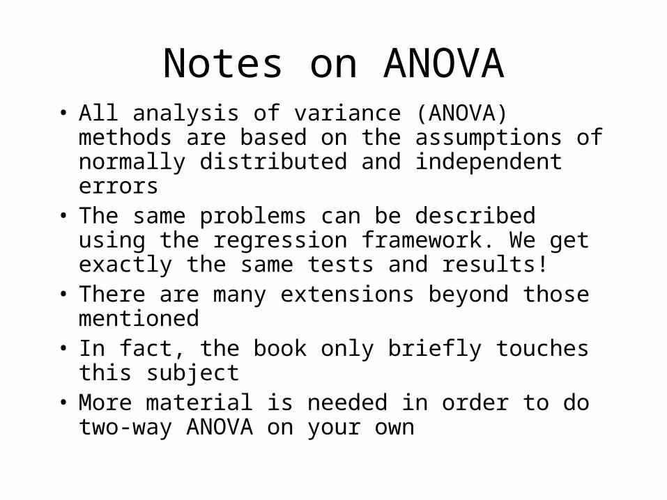
Notes on ANOVA• All analysis of variance (ANOVA) methods are

based on the assumptions of normally distributed and independent errors

• The same problems can be described using the regression framework. We get exactly the same tests and results!

• There are many extensions beyond those mentioned

• In fact, the book only briefly touches this subject• More material is needed in order to do two-way

ANOVA on your own

Next time:

• How to design a study? • Different sampling methods• Research designs• Sample size considerations

Documents

Analysis of variance