Comput Mech (2010) 45:141–156DOI 10.1007/s00466-009-0429-9

ORIGINAL PAPER

Analysis of plates and shells using an edge-based smoothed finiteelement method

Xiangyang Cui · Gui-Rong Liu · Guang-yao Li ·GuiYong Zhang · Gang Zheng

Received: 16 December 2008 / Accepted: 6 October 2009 / Published online: 23 October 2009© Springer-Verlag 2009

Abstract In this paper, an approach to the analysis ofarbitrary thin to moderately thick plates and shells by theedge-based smoothed finite element method (ES-FEM) ispresented. The formulation is based on the first order sheardeformation theory, and Discrete Shear Gap (DSG) method isemployed to mitigate the shear locking. Triangular meshesare used as they can be generated automatically for com-plicated geometries. The discretized system equations areobtained using the smoothed Galerkin weak form, and thenumerical integration is applied based on the edge-basedsmoothing domains. The smoothing operation can provide amuch needed softening effect to the FEM model to reduce thewell-known “overly stiff” behavior caused by the fully com-patible implementation of the displacement approach basedon the Galerkin weakform, and hence improve significantlythe solution accuracy. A number of benchmark problemshave been studied and the results confirm that the presentmethod can provide accurate results for both plate and shellusing triangular mesh.

X. Cui · G. Li (B) · G. ZhengState Key Laboratory of Advanced Design and Manufacturingfor Vehicle Body, Hunan University, 410082 Changsha, People’sRepublic of Chinae-mail: gyli@hnu.cn

X. Cui · G.-R. LiuDepartment of Mechanical Engineering, Centre for AdvancedComputations in Engineering Science (ACES),National University of Singapore, 9 Engineering Drive 1,Singapore 117576, Singaporee-mail: pwcuixy@gmail.com

G.-R. Liu · G. ZhangSingapore-MIT Alliance (SMA), E4-04-10, 4 Engineering Drive 3,Singapore 117576, Singapore

Keywords Smoothed Galerkin weak form ·Finite element · ES-FEM · Plate and shell · DSG

1 Introduction

Plates and shells are the most widely used structural compo-nents in civil, mechanical and aerospace engineering. In thepast several decades, the finite element method has been usedas a powerful numerical tool to simulate behaviors of platesand shells. Due to the complexity of the existing plate andshell elements, research on simpler, more efficient and inex-pensive plate and shell elements receives continuously stronginterest. Compared with quadrilateral element, triangular ele-ment is particularly attractive because of its simplicity, easyin automatic meshing and re-meshing in adaptive analysis.However, the development of effective triangular elementsfor plates and shell is not a trivial matter. The major difficul-ties are to overcome (1) the overly stiff behavior, and (2) theshear locking phenomenon.

Shear locking is a very well known phenomenon causedby parasitic internal energy leads to an additional, artifi-cial stiffness. Many efficient works have been done to over-come the shear locking and various triangular elements havebeen proposed. Pugh et al. [1] proposed a triangular platebending element with reduced integration. Belytschko et al.[2] used a single Gauss point integration for calculating theshear strain energy. However, the elements with reducedintegration or selective integration have low accuracy andoften exhibit zero energy modes. Moreover, they often cannot pass the patch test for thin plates. Discrete Kirchhofftriangular (DKT) elements were developed by Stricklin et al.[3] and Dhatt [4,5], where the shear locking was eliminatedby removing the shear deformation from element kinemat-ics. Efficient results were obtained using these elements only

123

142 Comput Mech (2010) 45:141–156

for thin structures since transverse shear flexibility cannotbe neglected in the analysis of thick shells. Batoz et al. [6]summarized the developments of flat triangular plate bend-ing elements with displacement degrees of freedom at thethree corner nodes, and concluded that only a few elementsare reliable in this class. Based on mixed interpolation of ten-sorial components (MITC), Bathe and co-workers developeda series of triangular elements [7,8]. MITC3 is a three-nodetriangular element which has a simple formulation, but somelocking is present in the solution of the clamped plate prob-lems and the hyperboloid shell problems [9]. Ayad et al. [10]proposed a MiSP (Mixed Shear Projected) approach basedon the Hellinger-Reissner variational principle. The shearstrains in this method were defined in terms of the edge tan-gential strains that were projected on the element degrees offreedom. Using assumed natural strains (ANS) model, Szeand Zhu [11] proposed a quadratic curved triangular shellelement, and Kim et al. [12,13] proposed a 3-node macrotriangular element for analysis of plates and shells. Chen andCheung [14] proposed two refined triangular thin/thick plateelements (DKTM and RDTKM) based on the Timoshenko’sbeam theory. Based on this work, Chen [15] proposed a15-DOF triangular discrete degenerated shell element.Bletzinger et al. [16] presented a 3-node non-isotropic tri-angular element DSG3 using the Discrete Shear Gap method(DSG). This element may be classified as an ANS element,but it needs not to choose an interpolation for the shear strainsor to specify any sampling points. It is based on the explicitsatisfaction of the kinematic equation for the shear strains atdiscrete points and effectively eliminates the parasitic shearstrains. This element is very simple and does not need tochoose an interpolation for the shear strains or to use addi-tional sampling points.

The overly stiff behavior is observed in all fully compat-ible displacement-based FEM models. The primary causeof the overly stiff behavior is the fully compatible imple-mentation of the assumed displacement field based on thestandard Galerkin weakform. The overly stiff behavior isparticularly severe when displacement-based triangular ele-ments is used, which often leads to very poor accuracy inthe solution. In order to reduce the stiffness of the modeland widen the solution space, Liu [17] proposed a general-ized smoothed Galerkin weak form (GS-Galerkin), revealedand proved a number of important properties including var-iational consistence, convergence, upper bound and softeneffects [18]. The smoothing operation [19] has been gen-eralized to include discontinuous functions [17], and is usedfor the gradient of field variables, and the smoothingoperations are performed in various ways for creating mod-els of desired properties. Using the node-based smoothingoperation and the point interpolation method for shape func-tion construction, a node-based smoothed point interpola-tion method (NS-PIM or LC-PIM [20]) was formulated. Liu

and Zhang [21] found that NS-PIM is variationally consis-tent when the solution is sought from a proper H space, andcan provide much better stress results. More importantly itcan provide upper bound solution in energy norm. Usingthe FEM shape function and the element-based smoothingoperations, a smoothed finite element method (SFEM) wasproposed [22]. The SFEM further divides the elements intosome smoothing domains, computes the integrals along theedge of the smoothing domains, and has been proven to haveexcellent properties. The SFEM of general n-sided polygonalelements has also been formulated, and works well for veryheavily distorted mesh [23]. Liu et al. [24] gave detailed the-oretical aspects including stability, bound property and con-vergence about SFEM. Cui et al. [25] extended the SFEM forlinear and nonlinear analysis of plates and shells. Nguyen-Xuan et al. [26] extend the SFEM for plate problem coupledwith MITC4 element [27]. All these models have a commonfoundation of the so-called G space theory [28], and fall intothe category of weakened weak (W2) formulation [18].

An edge-based smoothed finite element method(ES-FEM) [29,30] has been proposed for 2D solid mechan-ics problems using also the smoothed Galerkin weak formwith edge-based smoothing domains. It has been found thatthe simple change of smoothing domains gives the ES-FEMexcellent properties including good accuracy and free of spu-rious modes. In this work, the ES-FEM has been furtherextended to solve plates and shells. The present formula-tion is based on the first order shear deformation theory,and the shear locking is suppressed using DSG [16]. Thedomain is first discretized into a set of triangular elementsand linear shape functions are used as same as in the standardFEM. The smoothing domains associated with the edges ofthe triangles are then further formed and the system stiff-ness matrix is obtained by integrating numerically over eachsmoothing domains. Compared with FEM, the smoothingoperation reduces the stiffness of the discretized system, andcompensates nicely the “overly stiff” behavior of the FEMmodel. Hence, the ES-FEM can produce better solutions thancorresponding FEM model. For shell problems, an edge localcoordinate system is introduced for performing strainsmoothing operations. To validate the accuracy and stabilityof the present method, a number of numerical examples havebeen examined and comparisons are made with results avail-able in literatures. The excellent results have been obtainedfor both plate and shell problems.

2 Formulations

2.1 Basic equations for plate and shell

The first order shear deformation theory [31] is used in thiswork, and thus the displacements in Cartesian coordinatesystem can be expressed as follows

123

Comput Mech (2010) 45:141–156 143

u = u0 + zθy

v = v0 − zθx (1)

w = w0

where u0, v0 and w0 are the displacements of the mid-planeof the plate or shell in the x, y and z directions, θx and θy

denote the rotations respect to x and y directions, respec-tively.

The relevant strain vector ε can be written in terms of themid-plane deformations of Eq. (1), which gives

ε =

⎧⎪⎪⎪⎪⎨

⎪⎪⎪⎪⎩

εxx

εyy

γxy

γxz

γyz

⎫⎪⎪⎪⎪⎬

⎪⎪⎪⎪⎭

=

εm

0

+

εb

0

+

0εs

(2)

where εm the membrane strain, εb the bending strain (curva-ture), and εs the shear strain are given by

εm =

⎧⎪⎪⎪⎪⎪⎨

⎪⎪⎪⎪⎪⎩

∂u0

∂x∂v0

∂y∂u0

∂y+ ∂v0

∂x

⎫⎪⎪⎪⎪⎪⎬

⎪⎪⎪⎪⎪⎭

, εb =

⎧⎪⎪⎪⎪⎪⎨

⎪⎪⎪⎪⎪⎩

∂θy

∂x

−∂θx

∂y∂θy

∂y− ∂θx

∂x

⎫⎪⎪⎪⎪⎪⎬

⎪⎪⎪⎪⎪⎭

,

(3)

εs =

⎧⎪⎨

⎪⎩

∂w0

∂x+ θy

∂w0

∂y− θy

⎫⎪⎬

⎪⎭

Applying the principle of virtual work, the weak form isstated as follows∫

δεTmDmεmd +

∫

δεTb Dbεbd +

∫

δεTs Dsεsd

−∫

δuT fd −∫

δuT td = 0 (4)

where the membrane stiffness constitutive coefficients (Dm),the bending stiffness constitutive coefficients (Db) and thetransverse shear stiffness constitutive coefficients (Ds) aredefined as

Dm =t2∫

− t2

D0dz = tD0 (5)

Db =t2∫

− t2

z2D0dz = t3

12D0 (6)

Ds =t2∫

− t2

χG

[1 00 1

]

dz = χ tG

[1 00 1

]

(7)

in which G is shear modulus, χ = 5/6 is the shear correc-tion factor, and the matrix D0 is the constitutive coefficientsgiven by

D0 = E

1 − ν2

⎡

⎣1 ν 0ν 1 00 0 1 − ν/2

⎤

⎦ (8)

where E is Young’s modulus, and ν is Poisson ratio.The stresses can be given as follows,

σm = Nx , Ny, NxyT = Dmεm (9)

is the membrane force,

σ b = Mx , My, MxyT = Dbεb (10)

is the bending moment, and

σ s = Qx , QyT = Dsεs (11)

is the transverse shear force.At any point in a triangular element, the generalized dis-

placement field u in the element is interpolated using thenodal displacements at the nodes of the element by the linearshape functions. The same shape functions are used for bothdisplacements and rotations

u = u, v, w, θx , θyT = [N1 N2 N3]

⎧⎨

⎩

d1

d2

d3

⎫⎬

⎭(12)

where di = u0i , v0i , w0i , θxi , θyi T is the generalizednodal displacement at node i, Ni (x) is a diagonal matrix ofshape functions given by

Ni = diag Ni (x) , Ni (x) , Ni (x) , Ni (x) , Ni (x) (13)

in which Ni (x) is the shape function for node i . Since 3-nodetriangular element is used, the shape function is linear andcan be given as follows [32]

Ni (x) = ai + bi x + ci y

ai = 1

2Ae

(x j yk − xk y j

), bi = 1

2Ae

(y j − yk

), (14)

ci = 1

2Ae

(xk − x j

)

where Ae is the area of the triangular element, the subscripti varies from 1 to 3, j and k are determined by the cyclicpermutation in the order of i, j, k.

Substituting Eq. (12) into Eq. (3), the membrane strain εm

and the bending strain εb can be written as

εm = Bmd = [Bm1, Bm2, Bm3]

⎡

⎣d1

d2

d3

⎤

⎦ (15)

εb = Bbd = [Bb1, Bb2, Bb3]

⎡

⎣d1

d2

d3

⎤

⎦ (16)

123

144 Comput Mech (2010) 45:141–156

in which

Bmi =⎡

⎣Ni,x 0 0 0 00 Ni,y 0 0 0Ni,y Ni,x 0 0 0

⎤

⎦ (17)

Bbi =⎡

⎣0 0 0 0 Ni,x

0 0 0 −Ni,y 00 0 0 −Ni,x Ni,y

⎤

⎦ (18)

where “( ),” indicates differentiation, the subscript i = 1, 2, 3.

In order to eliminate the shear-locking, the “Discrete ShearGap” (DSG) method [16] is used here. In each triangularelement, the shear strain here can be given as:

γxz =3∑

i=1

Ni,x (x) wxi +3∑

i=1

Ni,x (x) wyi

γyz =3∑

i=1

Ni,y (x) wxi +3∑

i=1

Ni,y (x) wyi

(19)

where wxi and wyi are the discrete shear gaps at the nodei given by

wx1 = wx3 = wy1 = wy2 = 0

wx2 = (w2 − w1) − 1

2b (θx 1+θx 2)

+1

2a(θy1 + θy2

)(20)

wy3 = (w3 − w1) − 1

2d (θx 1 + θx 3) + 1

2c(θy1 + θy3

)

where

a = x2 − x1, b = y2 − y1

c = x3 − x1, d = y3 − y1(21)

From Eqs. (19), (20) and (21), the shear strain εs in eachelement can be written as

εs =

γxz

γyz

= Bsd = [Bs1, Bs2, Bs3]

⎧⎨

⎩

d1

d2

d3

⎫⎬

⎭(22)

in which

Bs1 = 1

2Ae

[0 0 b − d 0 Ae 00 0 c − a −Ae 0 0

]

(23a)

Bs2 = 1

2Ae

[0 0 d − bd

2ad2 0

0 0 −c bc2 − ac

2 0

]

(23b)

Bs3 = 1

2Ae

[0 0 −b bd

2 − bc2 0

0 0 a − ad2

ac2 0

]

(23c)

Γk

Edge k

Nodes of the element Centroid of the element

Ωk

Edge m Γm

Ωm

n1 n2

n3n4

n5n6

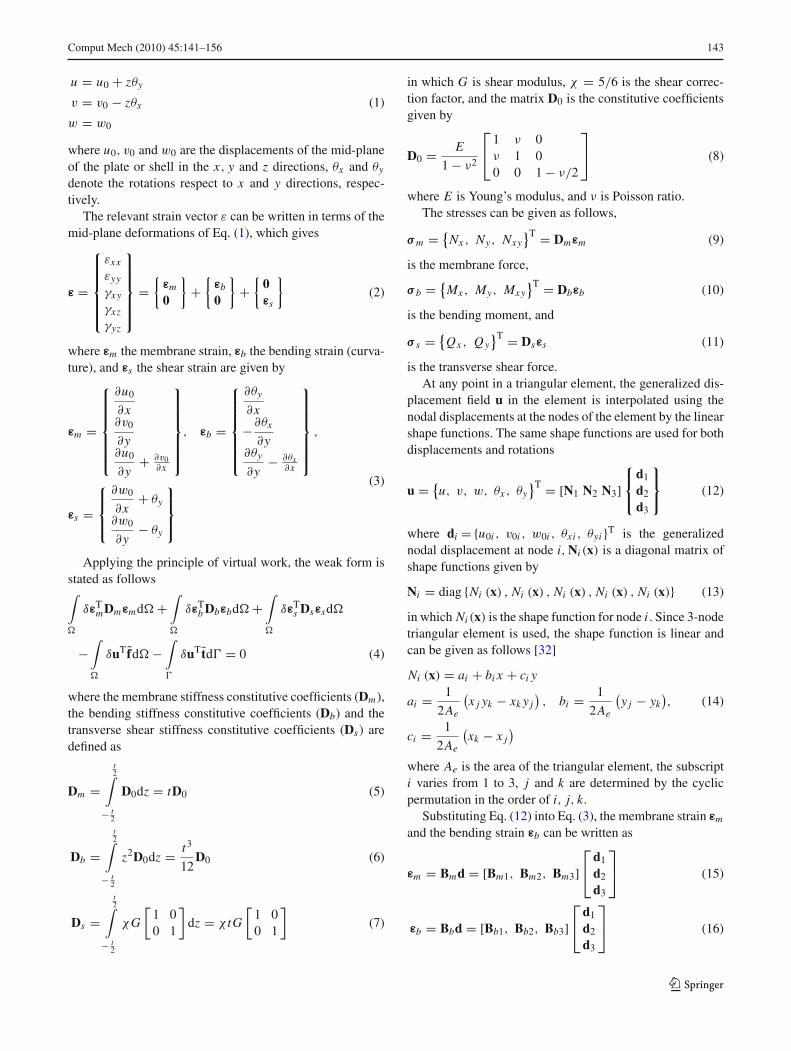
Fig. 1 A problem domain is divided into Neiem triangular elementswith a total of Nedge edges. Interior element edge k is sandwiched inthe smoothing domain k bounded by k . Smoothing domain m forthe boundary edge m is a triangle. There are Nk nodes that influencethe kth smoothing domain k . For domains associated with boundaryedges Nk = 3; for example, nodes n3, n5 and n6 influence m . Fordomains associated with interior edges Nk = 4; for example, nodesn1, n2, n3 and n4 influence k

2.2 Edge-based strain smoothing technique for plate

In this section, the edge-based strain smoothing techniquewill be introduced. In present ES-FEM, the problem domain is divided into Nelem triangular elements with a total ofNedge edges. In order to perform the smoothing operation, asmoothing domain for each edge is formed by sequentiallyconnecting two end points of the edge and centroids of its sur-rounding triangles, such that = 1 ∪2 ∪ . . .∪Nedge andi ∩ j = ∅, (i = j, i = 1, . . . , Nedge, j = 1, . . . , Nedge),as shown in Fig. 1. In the ES-FEM, the displacement inter-polation is element based, but the integration is based on thesmoothing domains. As shown in Fig. 2, for interior edges,the integration domain k of edge k is formed by assem-bling two sub-domains k1 and k2 of two neighboring ele-ments. The sub-domain k1 and the sub-domain k2 arefrom element e1 and element e2, respectively.

Introducing the strain smoothing operation [17], thesmoothed strain in the smoothing domain k are given by

ε(k)m = 1

Ak

∫

k

ε(k)m d

= 1

Ak

⎛

⎜⎝

∫

k1

ε(k1)m (x) d +

∫

k2

ε(k2)m (x) d

⎞

⎟⎠ (24a)

123

Comput Mech (2010) 45:141–156 145

Fig. 2 The integration isperformed over each of theedge-based smoothing domains.Domain k of edge k is formedby assembling two sub-domainsk1 and k2 of two neighboringelements. The sub-domain k1is from element e1 and thesub-domain k2 is from elemente2

Edge k

Γk

Edge k

ΩkΩk1

Ωk2

i m

j

nj

m

m

nj

i

element Nodes index

e1

e2

e2

e1

e1 i, j, me2 j, n, m

ε(k)b = 1

Ak

∫

k

ε(k)b d

= 1

Ak

⎛

⎜⎝

∫

k1

ε(k1)b (x) d +

∫

k2

ε(k2)b (x) d

⎞

⎟⎠ (24b)

ε(k)s = 1

Ak

∫

k

ε(k)s d

= 1

Ak

⎛

⎜⎝

∫

k1

ε(k1)s (x) d +

∫

k2

ε(k2)s (x) d

⎞

⎟⎠ (24c)

where Ak is the area of the smoothing domain k ,ε(k1)m (x), ε

(k1)b (x) and ε

(k1)s (x) are the compatible strains cal-

culated in element e1, ε(k2)m (x), ε

(k2)b (x) and ε

(k2)s (x) are the

compatible strain calculated in element e2.Since linear shape functions are used in the present

method, the compatible strain is a constant in each smoothingsub-domain. Therefore, Eq. (24) can be rewritten as

ε(k)m = 1

Ak

(Ak1ε

(k1)m + Ak2ε

(k2)m

)(25a)

ε(k)b = 1

Ak

(Ak1ε

(k1)b + Ak2ε

(k2)b

)(25b)

ε(k)s = 1

Ak

(Ak1ε

(k1)s + Ak2ε

(k2)s

)(25c)

where Ak1 and Ak2 are areas of the smoothing sub-domainsk1 and k2, respectively.

Substituting Eqs. (15), (16) and (22) into Eq. (25), thesmoothed strains can be given by

ε(k)m = Ak1

AkB(k1)

m d(k1) + Ak2

AkB(k2)

m d(k2) = B(k)m d(k) (26a)

ε(k)b = Ak1

AkB(k1)

b d(k1) + Ak2

AkB(k2)

b d(k2) = B(k)b d(k) (26b)

ε(k)s = Ak1

AkB(k1)

s d(k1) + Ak2

AkB(k2)

s d(k2) = B(k)s d(k) (26c)

Boundary line

m

Edge k

i

jΓ

Ω

k

k

Fig. 3 The integration domaink of edge k is only a single sub-domain

where d(k1) and d(k2) are the nodal displacements vectorof the element e1 and the element e2, respectively, d(k) arethe displacements vector of the nodes associated with edgek, B(k1)

m , B(k1)b and B(k1)

s are the compatible strain matrices of

the smoothing sub-domain k1 and B(k2)m , B(k2)

b and B(k2)s are

the compatible strain matrices of the smoothing sub-domaink2, respectively. Note that the sign ‘+’ denotes assemblybut not sum here.

For boundary edges as shown in Fig. 3, the smoothingdomain k of edge k is a single sub-domain, and strains inEq. (26) are obtained by the single subdomain. In this case,the strain and strain matrix have the same form as those inFEM.

2.3 Edge-based strain smoothing technique for shell

For shell problems, local coordinate system is defined in eachelement, and the compatible strains are computed in this localcoordinate system. In order to perform the strain smoothingover the same local coordinate system for two sub-domains

123

146 Comput Mech (2010) 45:141–156

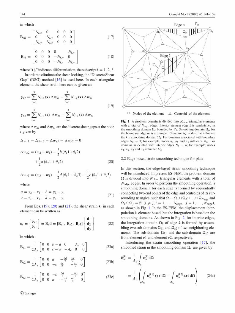
from two different elements sharing an inner edge, coordi-nate system (x, y, z) associated with an edge is defined inthis study. Let x be coinciding with the edge k, z be the aver-age normal direction of the two elements sharing edge k, andy direction is then defined as the cross product of the unitvectors in the z and x directions. From simple transforma-tion rules for each triangular element, the strain in the edgecoordinate system can be written as

εm = Rm1Rm2εm

εb = Rb1Rb2εb (27)

εs = Rs1Rs2εs

in which εm, εb and εs are strains in element local coordinatesystem, and

Rm1 = Rb1 =⎡

⎣

c2x x c2

x y c2x z cx x cx y cx ycxz cxx cxz

c2yx c2

y y c2yz cyx cyy cyycyz cyx cyz

2cxx cyx 2cx ycyy 2cxzcyz cxx cyy + cyx cx y cxzcyy + cyzcx y cxx cyz + cyx cxz

⎤

⎦ (28)

Rs1 =[

2cxx czx 2cx yczy 2cxzczz cxx czy + czx cx y cxzczy + czzcx y cxx czz + czx cxz

2cyx czx 2cyyczy 2cyzczz cyx czy + czx cyy cyzczy + czzcyy cyx czz + czx cyz

]

(29)

Rm2 = Rb2 =

⎡

⎢⎢⎢⎢⎢⎢⎢⎣

c2x x c2

yx cxx cyx

c2x y c2

y y cx ycyy

c2x z c2

yz cxzcyz

2cxx cx y 2cyx cyy cxx cyy + cx ycyx

2cx ycxz 2cyycy′z cx ycyz + cxzcyy

2cxx cxz 2cyx cy′z cxx cyz + cxzcyx

⎤

⎥⎥⎥⎥⎥⎥⎥⎦

(30)

Rs2 =

⎡

⎢⎢⎢⎢⎢⎢⎣

cxx czx cyx czx

cx yczy cyyczy

cxzczz cyzczz

cxx czy + cx yczx cyx czy + cyyczx

cxzczy + cx yczz cyzczy + cyyczz

cxx czz + cxzczx cyx czz + cyzczx

⎤

⎥⎥⎥⎥⎥⎥⎦

(31)

where as usual cxx is the cosine of the angle between the xand x axes, etc.

Using Eqs. (15), (16) and (22), the strains in the edge sys-tem can be obtained using those in element local coordinatesystem

εm = Rm1Rm2Bm d

εb = Rb1Rb2Bbd (32)

εs = Rs1Rs2Bs d

where Bm, Bb and Bs are strain matrices in element localcoordinate system, and

di = Tdi (33)

where di and di are the nodal displacement vectors at node iexpressed in local and global coordinates, respectively, and

transformation matrix T can be written as

T =[

T3×3 03×3

02×3 T2×3

]

(34)

in which

Ti j = cij (35)

As shown in Fig. 4, the smoothing domain k correspond-ing to an inner edge k consists of two sub-domains. The strainin the edge coordinate system of each sub-domain kI can benoted as ε(k I )

m , ε(k I )b and ε(k I )

s for the I th triangular element.As the strain is constant field in the linear triangular element,the strain in smoothing domain can be easily obtained by

ε(k)m = 1

Ak

∑

I

Ak I ε(k I )m (36a)

ε(k)b = 1

Ak

∑

I

Ak I ε(k I )b (36b)

ε(k)b = 1

Ak

∑

I

Ak I ε(k I )b (36c)

where Ak is the area of the smoothing domain k , Ak I is thearea of the sub-domain k I .

Using Eqs. (32), (33) and (36), the relationship betweenstrains and global nodal displacement vectors can begiven as

1e

1z

2z z

1x1y2x

2y xy

i

j

m

n

x

y

z

2e

edge k

Fig. 4 Shell element for edge-based smoothing, integration domainand coordinate systems

123

Comput Mech (2010) 45:141–156 147

ε(k)m = B(k)

m d(k) (37a)

ε(k)b = B(k)

b d(k) (37b)

ε(k)s = B(k)

s d(k) (37c)

in which

B(k)m = 1

Ak

∑

I

Ak I R(k)m1R(k I )

m2 B(k I )m T(I ) (38a)

B(k)b = 1

Ak

∑

I

Ak I R(k)b1 R(k I )

b2 B(k I )b T(I ) (38b)

B(k)s = 1

Ak

∑

I

Ak I R(k)s1 R(k I )

s2 B(k I )s T(I ) (38c)

where the summation in Eq. (38) means an assembly pro-cess, R(k)

m1, R(k)b1 and R(k)

s1 are the transformation matrices for

the kth edge given by Eqs. (28) and (29), R(k I )m2 , R(k I )

b2 , R(k I )s2

and T(k I ) are the transformation matrices for the I th elementsharing the edge k and they are given by Eqs. (30), (31) and(34). It must be pointed out that the global nodal displace-ments vector d(k) contains all of nodes of the two elementssharing the edge k.

2.4 Smoothed Galerkin formulation

We now seek for a weak form solution of generalized dis-placement field u that satisfies the following smoothedGalerkin weak form∫

δεTmDm εmd +

∫

δεTb Dbεbd +

∫

δεTs Ds εsd

−∫

δuT fd −∫

δuT td = 0 (39)

where f is the external load applied over the problem domain, and t is the traction applied on the natural boundary .

Substituting Eq. (12) and Eq. (26) (for plate) or Eq. (37)(for shell) into Eq. (39), a set of discretized algebraic systemequations can be obtained in the following matrix form

Kd − f = 0 (40)

where d is the vector of global nodal displacement at all ofthe nodes, and f is the force vector defined as

f =∫

N (x) fd +∫

N (x) td (41)

In Eq. (40), K is the (global) smoothed stiffness matrixassembled in the form of

Ki j =Nedge∑

k=1

K(k)i j (42)

The summation in Eq. (42) means an assembly processsame as the practice in the FEM, Nedge is the number of

the edges of the whole problem domain , and K(k)i j is the

stiffness matrix associated with edge k given as follows

K(k)i j = K(k)

mi j + K(k)bi j + K(k)

si j (43)

where

K(k)mi j =

∫

k

(B(k)

m

)T

iDm

(B(k)

m

)

jd

=(

B(k)m

)T

iDm

(B(k)

m

)

jAk

K(k)bi j =

∫

k

(B(k)

b

)T

iDb

(B(k)

b

)

jd

=(

B(k)b

)T

iDb

(B(k)

b

)

jAk

K(k)si j =

∫

k

(B(k)

s

)T

iDs

(B(k)

s

)

jd

=(

B(k)s

)T

iDs

(B(k)

s

)

jAk (44)

3 Numerical examples

3.1 Patch test

The first numerical example is the standard patch test; themesh of a square patch of the plate with thickness t = 0.001is depicted in Fig. 5. The plate is subjected to the prescribed

4 (0,10) (10,10)3

6 (8,9)

2 (10,0)

5 (3,4)

1 (0,0)

x

y

Fig. 5 Mesh for the standard patch test

123

148 Comput Mech (2010) 45:141–156

displacement and rotations on boundary of the patch (at nodes1 to 4) are computed using

w = 10−3(1 + x + y + x2 + xy + y2)

θx = −∂w

∂x= −10−3(1 + y + 2x) (45)

θy = −∂w

∂y= −10−3(1 + x + 2y)

The material properties of patch are E = 1.0 × 106 andν = 0.25. To satisfy the patch test, the deflection and rota-tions at any interior nodes computed by numerical methodshould be exactly the analytic ones given in Eq. (45). Toexamine the numerical error precisely, an error norm isdefined as

eu =√√√√

6∑

i=1

((ui

num − uiexact

)T (ui

num − uiexact

)

(ui

exact

)T (ui

exact

)

)

(46)

where unum is the displacement vector computed by the pres-ent ES-FEM, and uexact is the displacement vector computedfrom Eq. (45). Our numerical computation has found the errornorm being eu = 4.474065656539186 × 10−15 that is of the

order of the machine accuracy. This shows a successful passof the patch test for present method.

3.2 Square plates

A square plate of length L = 10 subjected to differentboundary conditions is considered in this subsection. Thematerial properties are taken as Young’s modulus E = 3.0×107, and Poisson ratio ν = 0.3. Owing to the symmetryconditions, only a quarter of the plate is modeled. Figure 6shows the meshes of different density used for the squareplate. The results of center deflections are normalized withthe formulation given by Zienkiewicz and Taylor [33]. Forthe plate subjected to uniform load, the deflection is normal-ized as w = wc D/q L4, where q is the uniform load. Forthe plate subjected to concentrated central load, the deflec-tion is normalized as w = wc D/P L2, in which P is theconcentrated central load. Both thin plate (L/t = 100) andthick plate (L/t = 5) with different boundary conditions areinvestigated in this subsection.

For the purpose of testing the element performance, thenumerical results obtained from the present ES-FEM arecompared with several existing triangular plate elements,

Fig. 6 Square plate mesh

2 elements per sidex

y

edis rep stnemele 8edis rep stnemele 4 6 elements per side

L

123

Comput Mech (2010) 45:141–156 149

Table 1 Numerical results ofnormalized central deflection fora simply supported square platesubjected uniform load(L/t = 100)

Mesh DKT RDKTM DSG Present

2 × 2 0.004056 0.004058 0.003705 0.004078

4 × 4 0.004065 0.004069 0.003975 0.004068

6 × 6 0.004064 0.004066 0.004024 0.004066

8 × 8 0.004064 0.004065 0.004042 0.004065

Analytic solution 0.004064

Table 2 Numerical results ofnormalized central deflection fora simply supported square platesubjected uniform load(L/t = 5)

Mesh DKT RDKTM DSG Present

2 × 2 0.004056 0.004902 0.004499 0.00496

4 × 4 0.004065 0.004904 0.004804 0.00492

6 × 6 0.004064 0.004906 0.00486 0.004912

8 × 8 0.004064 0.004906 0.004879 0.004909

Analytic solution 0.004907

Table 3 Numerical results ofnormalized central deflection fora clamped square plate subjecteduniform load (L/t = 100)

Mesh DKT RDKTM DSG Present

2 × 2 0.001547 0.00155 0.00107 0.00135

4 × 4 0.001347 0.00135 0.001213 0.001299

6 × 6 0.001303 0.001305 0.001243 0.001285

8 × 8 0.001287 0.001289 0.001254 0.001279

Analytic solution 0.001265

Table 4 Numerical results ofnormalized central deflection fora clamped square plate subjecteduniform load. (L/t = 5)

Mesh DKT RDKTM DSG Present

2 × 2 0.001547 0.002423 0.002226 0.001862

4 × 4 0.001347 0.002243 0.002205 0.002093

6 × 6 0.001303 0.002205 0.00219 0.002136

8 × 8 0.001287 0.002191 0.002183 0.002152

Analytic solution 0.00217

Table 5 Numerical results ofnormalized central deflection fora square plate subjectedconcentrated central load withdifferent constraints(L/t = 100)

Mesh Simply supported Clamped

DSG Present DSG Present

2 × 2 0.010624 0.011986 0.004252 0.005393

4 × 4 0.011285 0.011750 0.005205 0.005658

6 × 6 0.011445 0.011685 0.005416 0.005657

8 × 8 0.011507 0.011656 0.005496 0.005647

Analytic solution 0.011601 0.005612

123

150 Comput Mech (2010) 45:141–156

1 2 3 4 5 6 7 8 9-14

-12

-10

-8

-6

-4

-2

0

2

4

Mesh Density

Err

or in

Cen

tral

Def

lect

ion,

%

BCIZHSMDKTRDKTMDSGHCTPresent

1 2 3 4 5 6 7 8 9-25

-20

-15

-10

-5

0

5

10

15

Mesh Density

Err

or in

Cen

tral

Def

lect

ion,

%

DKTRDKTMDSGPresent

(a)

(b)

Fig. 7 Relative error of the deflection at centre for a simply supportedsquare plate with uniform load for different element types. a Thin plate(L/t = 100). b Thick plate (L/t = 5)

which include HCT [34], HSM [35], BCIZ [36], DKT [37],RDKTM [14] and DSG [16], and the analytic solutions gotfrom Ref. [31].

Numerical results of normalized central deflection for allcases are given in Tables 1, 2, 3, 4 and 5. The relative errorsof the results are plotted in Figs. 7, 8, and 9, in which the label“mesh density” of the horizontal axes refers to the numberof elements per side. From the results, it can be seen thatthe present method has a high accuracy and possesses fastconvergence for both the thick and thin plates with differ-ent boundary conditions. For all studied cases, the proposedES-FEM is not the best for each of the cases, but it is alwaysamong the bests for all these cases, which show clearly thestable and well-balanced feature of the ES-FEM. Note thatthe present method is very simple in formulation and noextra sampling points are introduced, compared with otherelements.

3.3 Shear locking test

A simply supported or clamped square plate subjected to auniform loading is used to test the shear locking phenom-enon. The geometry and material properties are as same as

1 2 3 4 5 6 7 8 9-25

-20

-15

-10

-5

0

5

10

15

20

25

Mesh Density

Err

or in

Cen

tral

Def

lect

ion,

%

BCIZHSMDKTRDKTMDSGHCTPresent

1 2 3 4 5 6 7 8 9-50

-40

-30

-20

-10

0

10

20

Mesh Density

Err

or in

Cen

tral

Def

lect

ion,

%

DKTRDKTMDSGPresent

(a)

(b)

Fig. 8 Deflection at centre for a clamped square plate with uniformload for different element types. a Thin plate (L/t = 100). b Thickplate (L/t = 5)

those used in the previous subsection. The deflection is nor-malized as w = wc D/q L4 and a 6 × 6 mesh is used here,and the computed results are plotted in Fig. 10. The resultsshow clearly that the proposed method can avoid shear lock-ing successfully and it provides excellent results regardlessof the thickness of the plate.

3.4 Circular plate

A simply supported or clamped circular plate subjected touniform loading is analyzed to demonstrate more features ofthe present method. The radius of the plate is R = 5 and twocases of the thickness, t = 0.1 and t = 1, are investigatedhere. Poisson ratio ν of the material is taken to be 0.3; Young’smodulus E of the material is 3 × 105. The configuration andmesh information of the plate are shown in Fig. 11, wherea quarter of the plate is modeled because of the symmetryconditions. A set of three meshes, 6, 24 and 96 elements, areemployed here. The boundary conditions are given by:

Simply supported: w = 0 on the boundary

Clamped: u = v = w = θx = θy = 0 on the boundary

(47)

123

Comput Mech (2010) 45:141–156 151

1 2 3 4 5 6 7 8 9-10

-5

0

5

Mesh Density

Err

or in

Cen

tral

Def

lect

ion,

%

BCIZHSMDSGHCTPresent

1 2 3 4 5 6 7 8 9-30

-25

-20

-15

-10

-5

0

5

10

Mesh Density

Err

or in

Cen

tral

Def

lect

ion,

%

BCIZHSMDSGHCTPresent

(a)

(b)

Fig. 9 Deflection at centre for a thin square plate (L/t = 100) withconcentrated central load for different element types subjected differentboundary. a Simply supported square plate. b Clamped square plate

102 10

410

6

4

4.5

5

5.5

6x 10

-3

Length/Thickness

Nor

mal

ized

Cen

tral

Def

lect

ion

AnalyticPresentThin Plate Solution (0.004062)

102 10

410

61

1.5

2

2.5

3

3.5x 10

-3

Length/thickness

Nor

mal

ized

Cen

tral

Def

lect

ion

AnalyticPresentThin Plate Solution (0.001265)

(a)

(b)

Fig. 10 Shear locking test. a simply supported square plate. b Clampedsquare plate

Fig. 11 Circular plate withuniform load. Geometry andMesh arrangements

t

R=5

x

yz

6 elements 24 elements 96 elements

Boundary conditionsSimply supported:w=0 Clamped:u=v=w= x= y=0

123

152 Comput Mech (2010) 45:141–156

0 10 20 30 40 50 60 70 80 90 1000.84

0.86

0.88

0.9

0.92

0.94

0.96

0.98

1

1.02

Element number

wc/w

ref

PresentMiSP3DKTDSGRDKTMDST-BKDST-BL 95 95.5 96

0.993

0.994

0.995

0.996

0.997

0 10 20 30 40 50 60 70 80 90 1000.86

0.88

0.9

0.92

0.94

0.96

0.98

1

1.02

1.04

1.06

Element number

wc/w

ref

PresentMiSP3DKTDSGRDKTMDST-BKDST-BL 95 95.5 96

0.995

1

1.005

(a)

(b)

Fig. 12 Deflection at centre for a thin circular plate (t/R = 0.02) withuniform load for different element types. a Simply supported plate.b Clamped plate

For a simply supported or clamped thin circular platesubjected to uniform load q0; the analytic solutions for cen-tral deflections w and moment Mr are given by [37]

Simply supported:w = q0 R4

64D

(5+v1+v

+ 83k(1−v)

( tR

)2)

Mr = q0 R2

16 (3 + v) (48)

Clamped:w = q0 R4

64D

(1 + 8

3k(1−v)

( tR

)2)

Mr = q0 R2

16 (1 + v)(49)

where D = Et3/(12(1 − ν2)) is the bending stiffness.Numerical results of the present method are compared

with those of existing triangular elements, which includeDKT [37], RDKTM [14], BST-BK [38], BST-BL [39],MiSP3 [10], and DSG [16]. Numerical results of normalizedcentral deflection wc/wref , in which wref is analytic results inEqs. (48) and (49) for the thin plate (t/R = 0.02) are plottedagainst the elements number in Fig. 12. The results of centralmoment are plotted in Fig. 13. These two pictures show thatthe present method can produce very accurate results whenthe problem domain is descritized using a reasonably num-ber of elements (24 and 96 elements for this case). When

0 10 20 30 40 50 60 70 80 90 100

4.2

4.4

4.6

4.8

5

5.2

5.4

Element number

Mc

Reference (5.15625)PresentDKTDSGRDKTMDST-BKDST-BL 95 95.5 96

5.12

5.14

5.16

5.18

5.2

0 10 20 30 40 50 60 70 80 90 100

1.4

1.6

1.8

2

2.2

2.4

Element number

Mc

Reference (2.03125)PresentDKTDSGRDKTMDST-BKDST-BL 95 95.5 96

2.02

2.04

2.06

2.08

2.1

(a)

(b)

Fig. 13 Moment at centre for a thin circular plate (t/R = 0.02) withuniform load for different element types. a Simply supported plate.b Clamped plate

too few elements are used (6 elements for this case), resultsof the present method are found only better than the plainelements also using DSG to eliminate shear locking. Thisis because the ES-FEM relies on the sufficient number ofedges for the smoothing operation to take effects. When themodel has too few edges, it has no much difference comparedto the plain elements. For the case of 6 elements, there aretotally 12 edges and only half of them (6 interior edges) arebeing effectively smoothed. Therefore, we are not expectingan outstanding performance of the ES-FEM for this case. Thisfounding agrees with those methods using smoothed Galer-kin formulations [17]. With the increase of the number ofelements (e.g., 24 and 96 elements), the ES-FEM clearly outperforms other elements. Note that in any practical problems,we use a lot more than tens of elements, and hence ES-FEMis expected to perform well in solving actual problems.

A clamped thin (t/R = 0.02) and thick (t/R = 0.2)circular plates subjected to a uniform load are analyzed toobtain the distributed bending moments (Mr , Mθ ) and shearforce (Tr ). The mesh of 96 elements is employed, and thenumerical results of present method are shown in Figs. 14, 15and 16, together with the results obtained using BST-BK[38], BST-BL [39] and MiSP3 [10] with the same mesh.

123

Comput Mech (2010) 45:141–156 153

0 0.5 1 1.5 2 2.5 3 3.5 4 4.5 5-4

-3

-2

-1

0

1

2

3

r

Mr

ReferencePresentDST-BKDST-BLMiSP3

0 0.5 1 1.5 2 2.5 3 3.5 4 4.5 5-4

-3

-2

-1

0

1

2

3

r

Mr

ReferencePresentDST-BKDST-BLMiSP3

(a)

(b)

Fig. 14 Moment Mr along the radius for a clamped circular plate withuniform load. a Thin plate (t/R = 0.02). b Thick plate (t/R = 0.2)

The analytic solutions are given by [40] as follows

Mr (r) = q0

16

[(1 + v) R2 − (3 + ν) r2

]

Mθ (r) = q0

16

[(1 + v) R2 − (1 + 3ν) r2

](50)

Tr (r) = −q0r

2

where r is the distance gauged from the plate center, andD = Et3/(12(1 − ν2)) is the bending stiffness.

Nodal values of Mr , Mθ and Tr for present method areobtained by averaging the values of the associated smooth-ing domains. The forces of the MiSP3 element are computedat the nodes, and the forces of BST-BL and BST-BK elementsare computed at the centroids of the elements. It is found thatthe present method performs among the best for all the casesof both thin and thick plates. For bending moments, numer-ical results of all the methods studied here are all in goodagreement with the reference solutions. For shear forces, thepresent method and MiSP3 element provide more accurateresults compared with other numerical methods.

0 0.5 1 1.5 2 2.5 3 3.5 4 4.5 5-1.5

-1

-0.5

0

0.5

1

1.5

2

2.5

r

M

ReferencePresentDST-BKDST-BLMiSP3

0 0.5 1 1.5 2 2.5 3 3.5 4 4.5 5-1

-0.5

0

0.5

1

1.5

2

2.5

r

M

ReferencePresent(EST)DST-BKDST-BLMiSP3

(a)

(b)

Fig. 15 Moment Mθ along the radius for a clamped circular plate withuniform load. a Thin plate (t/R = 0.02). b Thick plate (t/R = 0.2)

3.5 Pinched cylinder with end diaphragms

A pinched cylinder supported at each end by rigid diaphragmshown in Fig. 17 is considered in this section. It is a widelyused benchmark problem for determining the ability of theelements to represent inextensional bending and complexmembrane states. The length of the pinched cylinder is L =600 in., the radius is R = 300 in., and the thickness ist = 3 in. The material properties are: Poisson’s ratio υ = 0.3,and Young’s modulus E = 3.0 × 106 N/in.2. The loading isa pair of pinching loads P = 100 N. Owing to the sym-metry, only 1/8 of the problem is modeled. Five meshes,4 × 4, 6 × 6, 8 × 8, 12 × 12 and 16 × 16, are examined hereand only the 4 × 4 mesh is shown in Fig. 17. In this case, theanalytical solution of the radial displacement under the pointload is 0.0018248 in., and the solutions given in this case arenormalized with this value. Numerical results of the presentmethod are compared with those of existing triangular shellelements ANS6S [11], C0 [41], DSG3 [16] and S3R elementin ABAQUS©. From the results given in Table 6, it can beseen that the proposed element provides accurate results andhas a good convergence performance.

123

154 Comput Mech (2010) 45:141–156

0 1 2 3 4 5 60

0.5

1

1.5

2

2.5

3

3.5

4

r

Tr

ReferencePresentDST-BKDST-BLMiSP3

0 1 2 3 4 5 60

0.5

1

1.5

2

2.5

3

r

Tr

ReferencePresentDST-BKDST-BLMiSP3

(a)

(b)

Fig. 16 Shear force Tr along the radius for a clamped circular platewith uniform load. a Thin plate (t/R = 0.02). b Thick plate (t/R = 0.2)

diaphragm

100P =

100P =

L

,z w

,y v

,x u

R

t

diaphragm

Fig. 17 Pinched cylinder with end diaphragms, 4 × 4 mesh illustrated

3.6 Hemispherical shell

The hemispherical shell with an 18 hole is loaded anti-symmetrically by point loads as shown in Fig. 18. It exhibitsalmost no membrane strains but it is a challenging test onthe ability of an element to handle rigid body rotations aboutnormals to the shells surface. The geometric parameters areradius R = 10 m and thickness t = 0.04 m. The material

Table 6 Pinched cylinder with end diaphragms; normalized displace-ment at load point (the value used for normalization is 0.0018248 in)

Mesh 4 × 4 6 × 6 8 × 8 12 × 12 16 × 16

ANS6S 0.502 0.741 0.857 0.955 0.985

S3R 0.550 – 0.801 0.897 0.937

C0 0.300 0.530 0.670 – –

DSG 0.313 0.548 0.690 0.832 0.897

Present 0.421 0.674 0.806 0.924 0.972

z

x

y

1.0F =

1.0F =

18°

Sym

Sym

Fig. 18 Pinched cylindrical with end diaphragms, five nodes per sideillustrated

Table 7 Hemispherical shell; normalized displacement at load point(the value used for normalization is 0.093 m)

Mesh 4 × 4 6 × 6 8 × 8 12 × 12 16 × 16

ANS6S 0.949 – 0.982 0.995 1.001

S3R 0.357 – 0.913 0.968 0.981

C0 0.870 0.930 0.960 – –

DSG 0.965 0.977 0.981 0.986 0.989

Present 1.021 1.010 1.004 1.002 1.002

properties are: Poisson’s ratio υ = 0.3, and Young’s mod-ulus E = 6.825 × 107 Pa. The point loading is F = 1 N.The solutions are obtained by using five meshes including4 × 4, 6 × 6, 8 × 8, 12 × 12 and 16 × 16. A typical 4 × 4mesh is shown in Fig. 18. The analytical radial deflectioncoincident at point load is 0.093 m, and the solutions givenin Table 7 are normalized with this value. It can be observedthat the present results agree well with analytic solutions.

3.7 Hood of an automobile

Finally, an actual structure component of a car hood shown inFig. 19 is studied using the present element. The dent resis-

123

Comput Mech (2010) 45:141–156 155

Fig. 19 Model of the hood of an automobile

1000 2000 3000 4000 5000 6000 70000.2

0.3

0.4

0.5

0.6

0.7

0.8

0.9

1

Node number

Dis

plac

emen

t at l

oad

poin

t

Reference (ABAQUS Quad with 25423 nodes)PresentABAQUS

Fig. 20 Displacements in x-direction at the loading point

tance of car hood is one of the important considerations inthe process of car design. In this example, all of the bound-ary nodes are fixed, and a concentrated load F = 150 Nis imposed along the x-direction. The thickness of the thinshell is 0.8 mm; Poisson’s ratio of the material is taken to be0.3; Young’s modulus of the material is 2.1×105‘N/ mm2. Inorder to test the accuracy of the present element, the solutionsof triangular element S3R in ABAQUS© is used for compar-ison. The reference solution is obtained using quadrilateralshell elements in ABAQUS© with large number of (25,423)nodes. Figure 20 shows that the present triangular elementhas a much higher accuracy than triangular shell elementsused in the ABAQUS©.

4 Conclusions

In this paper, an edge-based smoothed finite element methodis formulated to analyze plates and shells using simple 3-node triangular elements. The smoothed Galerkin weak formis used for discretizing the system equations and the numeri-cal integration is performed based on the smoothing domainsassociated with edges of the mesh. The Discrete Shear Gapmethod (DSG) is employed to mitigate the shear locking

effect. Numerical results of plate and shell problems haveconfirmed the following features of the present method.

1. The conventional 3-node triangular element is used in theES-FEM. There is no extra sampling point introducedto evaluate the stiffness matrix in present formulation.Hence the present method is very simple and can be eas-ily implemented with little changes to the FEM code.

2. Compared with fully compatible displacement-based andhence overly stiff finite element, the present method canprovide a much needed softening effect to the modelowing to the edge-based gradient smoothing operation.Therefore, the performance of the present method isgreatly enhanced.

3. The present method can pass exactly the pure bendingpatch test which ensures numerically the convergence ofthe proposed method.

4. Numerical comparisons show that the present elementcan obtain very stable and accurate results.

Acknowledgments The support of National 973 project (2010CB-328005), National Outstanding Youth Foundation (50625519), Key Pro-ject of National Science Foundation of China (60635020), Programfor Changjiang Scholar and Innovative Research Team in Universityand the China-funded Postgraduates’ Studying Abroad Program forBuilding Top University are gratefully acknowledged. The authors alsogive sincerely thanks to the partition financial support by the A*StarSingapore and the Centre for ACES, Singapore-MIT Alliance (SMA),and National University of Singapore.

References

1. Pugh ED, Hinton E, Zienkiewicz OC (1978) A study of triangu-lar plate bending element with reduced integration. Int J NumerMethods Eng 12:1059–1078

2. Belytschko T, Stolarski H, Carpenter N (1984) A C0 triangularplate element with one-point quadrature. Int J Numer MethodsEng 20:787–802

3. Stricklin J, Haisler W, Tisdale P, Gunderson R (1969) A rapidlyconverging triangular plate bending element. AIAA J 7:180–181

4. Dhatt G (1969) Numerical analysis of thin shells by curved tri-angular elements based on discrete Kirchhoff hypothesis. In: Pro-ceedings of the ASCE symposium on applications of FEM in civilengineering. Vanderbilt University, Nashville, pp 255–278

5. Dhatt G (1970) An efficient triangular shell element (Kirchhofftriangular shell element design via linear shell theory). AIAA J.8:2100–2102

6. Batoz JL, Bathe KJ, Ho LW (1980) A study of three-node trian-gular plate bending elements. Int J Numer Methods Eng 15:1771–1812

7. Bathe KJ, Brezzi F (1989) The MITC7 and MITC9 plate bendingelement. Comput Struct 32:797–814

8. Lee PS, Bathe KJ (2004) Development of MITC isotropic triangu-lar shell finite elements. Comput Struct 82:945–962

9. Lee PS, Noh HC, Bathe KJ (2007) Insight into 3-node triangu-lar shell finite element: the effects of element isotropy and meshpatterns. Comput Struct 85:404–418

123

156 Comput Mech (2010) 45:141–156

10. Ayad R, Dhatt G, Batoz JL (1998) A new hybrid-mixed varia-tional approach for Reissner–Mindlin plates, the MiSP model. IntJ Numer Methods Eng 42:1149–1479

11. Sze KY, Zhu D (1999) A quadratic assumed natural strain shellcurved triangular element. Comp Methods Appl Mech Eng 174:57–71

12. Kim JH, Kim YH (2002) Three-node macro triangular shell ele-ment based on the assumed natural strains. Comput Mech 29:441–458

13. Kim JH, Kim YH (2002) A three-node C0 ANS element for geo-metrically non-linear structural analysis. Comp Methods ApplMech Engrg 191:4035–4059

14. Chen WJ, Cheung YK (2001) Refined 9-Dof triangular Mindinplate elements. Int J Numer Methods Eng 51:1259–1281

15. Chen WJ (2004) Refined 15-DOF triangular discrete degeneratedshell element. Int J Numer Methods Eng 60:1817–1846

16. Bletzinger KU, Bischoff M, Ramm E (2000) A unified approachfor shear-locking-free triangular and rectangular shell finite ele-ments. Comput Struct 75:321–334

17. Liu GR (2008) A generalized gradient smoothing technique andsmoothed bilinear form for Galerkin formulation of a wide classof computational methods. Int J Comput Methods 5(2):199–236

18. Liu GR (2009) A G space theory and weakened weak (W2) form fora unified formulation of compatible and incompatible methods, PartI: theory and part II: applications to solid mechanics problems. IntJ Numer Methods Eng. doi:10.1002/nme.2719 (published online)

19. Chen JS, Wu CT, Yoon S, You Y (2001) A stabilized conform-ing nodal integration for Galerkin meshfree methods. Int J NumerMethods Eng 50:435–466

20. Liu GR, Zhang GY, Dai KY, Wang YY, Zhong ZH, Li GY,Han X (2005) A linearly conforming point interpolation method(LC-PIM) for 2D solid mechanics problems. Int J ComputMethods 2:645–665

21. Liu GR, Zhang GY (2008) Upper bound solution to elasticity prob-lems: A unique property of the linearly conforming point interpo-lation method (LC-PIM). Int J Numer Methods Eng 74:1128–1161

22. Liu GR, Dai KY, Nguyen TT (2007) A smoothed finite elementmethod for mechanics problems. Comput Mech 39:859–877

23. Dai KY, Liu GR, Nguyen TT (2007) An n-sided polygonalsmoothed finite element method (nSFEM) for solid mechanics.Finite Elem Anal Des 43:847–860

24. Liu GR, Nguyen TT, Dai KY, Lam KY (2007) Theoretical aspectsof the smoothed finite element method (SFEM). Int J Numer Meth-ods Eng 71:902–930

25. Cui XY, Liu GR, Li GY, Zhao X, Nguyen TT, Sun GY (2008) Asmoothed finite element method (SFEM) for linear and geometri-cally nonlinear analysis of plates and shells. CMES Comput ModelEng Sci 28(2):109–126

26. Nguyen-Xuan H, Rabczuk T, Bordas S, Debongnie JF (2008) Asmoothed finite element method for plate analysis. Comp MethodsAppl Mech Eng 197:1184–1203

27. Bathe KJ, Dvorkin EH (1985) A four-node plate bending elementbased on Mindlin–Reissner plate theory and mixed interpolation.Int J Numer Methods Eng 21:367–383

28. Liu GR (2009) On the G space theory. Int J Comput Methods6(2):257–289

29. Liu GR, Nguyen TT, Dai KY, Lam KY (2008) An edge-basedsmoothed finite element method (ES-FEM) for static, free andforced vibration analysis. J Sound Vib 320:1100–1130

30. Cui XY, Liu GR, Li GY, Zhang GY, Sun GY (2009) Analysis ofelastic–plastic problems using edge-based smoothed finite element.Int J Press Vessel Pip 86:711–718

31. Timoshenko S, Woinowsky-Krieger S (1940) Theory of plates andshells. McGraw-Hill, New York

32. Liu GR, Quek SS (2003) The finite element method: a practicalcourse. Butterworth Heinemann, Oxford

33. Zienkiewicz OC, Taylor RL (2000) The finite element method. In:Solid Mechanics, 5th edn, vol. 2. Butterworth-Heinemann, Oxford

34. Clough RW, Tocher JL (1965) Finite element stiffness matricesfor analysis of plates in bending. In: Proceedings of conferenceon matrix methods in structural mechanics. Air Force Institute ofTechnology, Wright-Patterson A. F. Base, Ohio, pp 515–545

35. Alwood RJ, Cornes GM (1969) A polygonal finite element forplate bending problems using the assumed stress approach. Int JNumer Methods Eng 1:135–149

36. Bazeley GP, Cheung YK, Irons BM, Zienkiewicz OC (1965) Tri-angular elements in plate bending conforming and non-conform-ing solutions. In: Proceedings of conference on matrix methods instructural mechanics. Air Force Institute of Technology, Wright-Patterson A. F. Base, Ohio, pp 547–577

37. Batoz JL (1982) An explicit formulation for an efficient triangularplate-bending element. Int J Numer Methods Eng 18:1077–1089

38. Batoz JL, Katili I (1992) On a simple triangular Reissner/Mindlin plate element based on incompatible modes and discreteconstraints. Int J Numer Methods Eng 35:1603–1632

39. Batoz JL, Lardeur P (1989) A discrete shear triangular nine dofelement for the analysis of thick to very thin plates. Int J NumerMethods Eng 28:533–560

40. Ugural AC (1981) Stresses in plates and shells. McGraw-Hill,New York

41. Belytschko T, Stolarski H, Carpenter NA (1984) C0 triangularplate element with one point quadrature. Int J Numer MethodsEng 20:787–862

123