Analysis of Plasma Detachment through Magnetic Nozzle via

Canonical Field Theory

Yu Takagaki

A thesissubmitted in partial fulfillment of the

requirements for the degree of

Master of Science in Aeronautics and Astronautics

University of Washington

2017

Committee

Setthivoine You

Uri Shumlak

Program Authorized to Offer Degree:

Aeronautics and Astronautics

c⃝Copyright 2017

Yu Takagaki

University of Washington

Abstract

Analysis of Plasma Detachment through Magnetic Nozzle via Canonical Field Theory

Yu Takagaki

Chair of the Supervisory Committee:

Assistant Professor Setthivoine You

Aeronautics and Astronautics

In this paper, I have investigated the mechanism of plasma detachment through magnetic

nozzle via canonical field theory, especially by considering canonical vorticity flux Ψσ contour

and dissipative force Rσ. As one of the most recent experimental proofs of plasma detach-

ment, Olsen et al[5]., observed and investigated three key indications of plasma detachment.

However, after solving for numerical fits with their experimental data, I found that constant

ion flux lines did not actually separate from constant magnetic flux lines. Thus, their first

key indication becomes incorrect now. Whereas, my analytical results are consistent with

the other two key indications. At the beginning, plasma detached from canonical vorticity

flux contours due to non-zero dissipative force and attached on magnetic flux lines instead.

However, Rσ ≃ 0 force makes plasma re-attach on canonical vorticity flux contours around

the plume edge region. As the most significant and notable result through my analysis, I

confirmed the existence of returning plasma flow around the plume edge region.

TABLE OF CONTENTS

Page

List of Tables . . . . . . . . . . . . . . . . . . . . . . . . . . . . . . . . . . . . . . . . iii

List of Figures . . . . . . . . . . . . . . . . . . . . . . . . . . . . . . . . . . . . . . . iv

Chapter 1: Introduction . . . . . . . . . . . . . . . . . . . . . . . . . . . . . . . . 1

Chapter 2: Overview of Plasma Detachment through Magnetic Nozzle . . . . . . . 3

2.1 What is Plasma Detachment . . . . . . . . . . . . . . . . . . . . . . . . . . . 3

2.2 Historical Research Progress on Magnetic Nozzle and Plasma Detachment . . 4

Chapter 3: Plasma Detachment observed in VASIMR Research . . . . . . . . . . . 8

3.1 Experimental Setup . . . . . . . . . . . . . . . . . . . . . . . . . . . . . . . . 8

3.2 Experimental Results and Discussion . . . . . . . . . . . . . . . . . . . . . . 10

3.3 Summary of VASIMR VX-200 Research . . . . . . . . . . . . . . . . . . . . 18

Chapter 4: Canonical Field Theory . . . . . . . . . . . . . . . . . . . . . . . . . . 19

4.1 Governing Equations . . . . . . . . . . . . . . . . . . . . . . . . . . . . . . . 20

4.2 Frozen-in Theorem for Canonical Field Theory . . . . . . . . . . . . . . . . . 21

Chapter 5: Analysis of Plasma Detachment via Canonical Field Theory . . . . . . 24

5.1 Constant Ion Flux Contour . . . . . . . . . . . . . . . . . . . . . . . . . . . 24

5.2 Canonical Vorticity Flux Contour . . . . . . . . . . . . . . . . . . . . . . . . 29

5.3 Summary of Analysis . . . . . . . . . . . . . . . . . . . . . . . . . . . . . . . 33

Chapter 6: Summary . . . . . . . . . . . . . . . . . . . . . . . . . . . . . . . . . . 35

Appendix A: Frozen-in Theorem . . . . . . . . . . . . . . . . . . . . . . . . . . . . . 37

i

Appendix B: Constant Γiz (redge) case . . . . . . . . . . . . . . . . . . . . . . . . . . 38

Bibliography . . . . . . . . . . . . . . . . . . . . . . . . . . . . . . . . . . . . . . . . 40

ii

LIST OF TABLES

Table Number Page

4.1 Comparison of governing equations between MHD Theory and Canonical FieldTheory . . . . . . . . . . . . . . . . . . . . . . . . . . . . . . . . . . . . . . . 22

4.2 One-to-one relationships between MHD Theory and Canonical Field Theory 23

iii

LIST OF FIGURES

Figure Number Page

3.1 Conceptual schematic of VASIMR VX-200 engine[5] . . . . . . . . . . . . . . 9

3.2 Image of plasma diagnostics[5] . . . . . . . . . . . . . . . . . . . . . . . . . . 10

3.3 ”Illustrating the method of spatially tracking lines of constant integrated ionflux and magnetic flux. Convergent detachment is shown (x-section insets)and appears as ion flux (pink) expanding slower than magnetic flux (blue)”[5]. 11

3.4 ”Standard shot configuration including uncertainty bounds (dashed lines).Data analysis windows for the low- and high-power configurations were takenfrom 0.4‒ 0.5 and 0.65‒ 0.75 s, respectively. Top: average RF forward powerprofile. Middle: steady 3600-sccm (~ 107 mg/s) argon flow. Bottom: exhaustregion chamber pressure measured by separate hot cathode ion gauges.”[5] . 13

3.5 Lines of constant fi (red solid) during the helicon + ICH operation comparedwith lines of constant enclosed magnetic flux (black dashed)[5] . . . . . . . . 14

3.6 Possible shapes of plasma plume and redge . . . . . . . . . . . . . . . . . . . 15

3.7 Contour maps of the ion velocity distribution function as a function of vr andvz at five radial locations and z = 3.9 [m]. ”The local magnetic field vector isoverlain in each plot (black arrow)”[5] . . . . . . . . . . . . . . . . . . . . . . 16

3.8 ”Image summarizing various regions associated with detachment process. Theflow lines (blue) are based on the integrated ion flux fraction and extended outalong the linear region. Lines showing the transition above unity for kineticand thermal beta are displayed for reference (red dashed)”[5] . . . . . . . . . 17

5.1 Comparison for the strength of magnetic field on z-axis for vacuum case(black), helicon only case (blue), and helicon + ICH case (red) in experimentsand my analytical one (green)[5] . . . . . . . . . . . . . . . . . . . . . . . . . 25

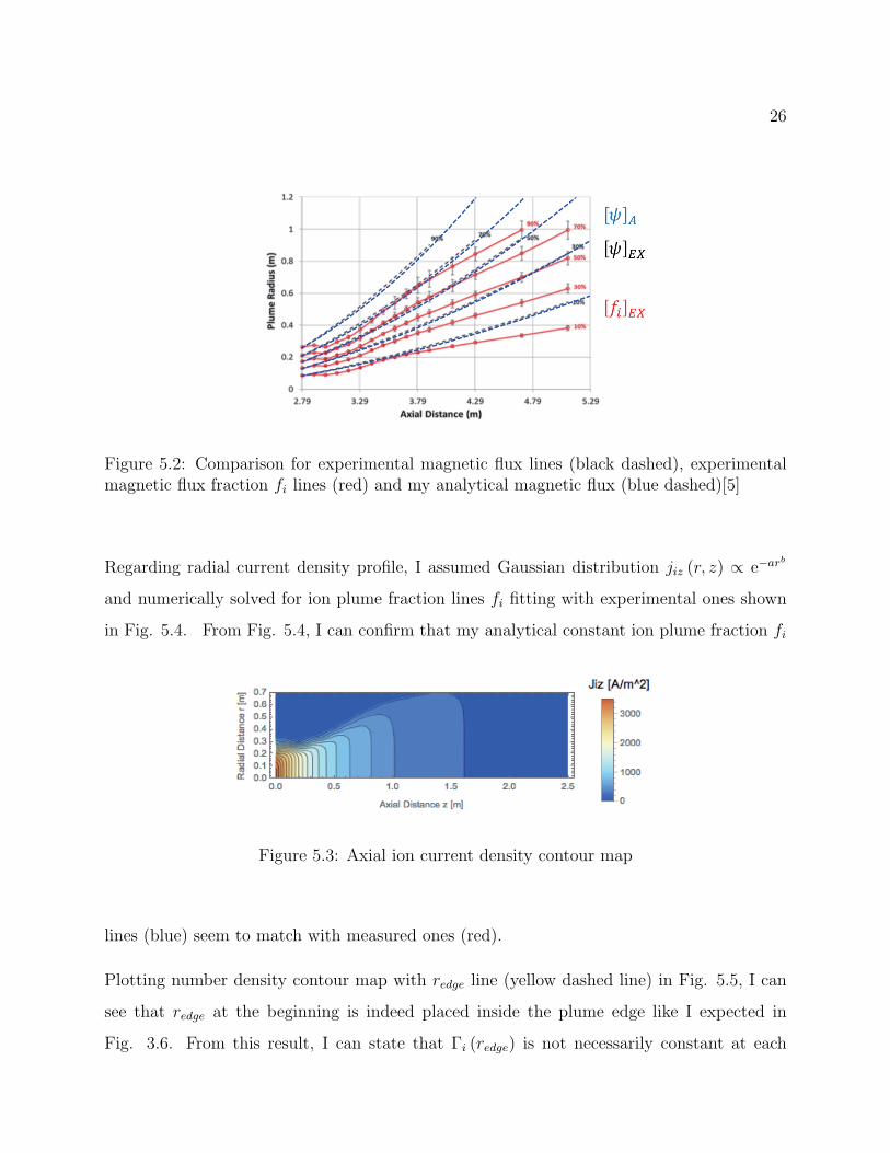
5.2 Comparison for experimental magnetic flux lines (black dashed), experimentalmagnetic flux fraction fi lines (red) and my analytical magnetic flux (bluedashed)[5] . . . . . . . . . . . . . . . . . . . . . . . . . . . . . . . . . . . . . 26

5.3 Axial ion current density contour map . . . . . . . . . . . . . . . . . . . . . 26

iv

5.4 Comparison between experimental ion flux fraction fi lines (red) and my an-alytical fi lines (blue) with experimental magnetic flux ψ lines (black dashed)and analytical magnetic flux ψ lines (light blue dashed)[5] . . . . . . . . . . 27

5.5 number density contour map with redge (yellow dashed). Red point indicatesthe basepoint of redge . . . . . . . . . . . . . . . . . . . . . . . . . . . . . . . 27

5.6 number density contour map with redge (yellow dashed). Red point indicatesthe basepoint of redge . . . . . . . . . . . . . . . . . . . . . . . . . . . . . . . 28

5.7 ni contour map with constant ion flux Γi (r) lines (blue solid), constant mag-netic flux ψ lines (light blue dashed), and redge (yellow dashed) . . . . . . . . 29

5.8 ni contour map with constant canonical vorticity flux Ψi lines (orange), con-stant ion flux Γi (r) lines (blue), constant magnetic flux ψ lines (light bluedashed), and redge (yellow dashed) . . . . . . . . . . . . . . . . . . . . . . . . 31

5.9 Summary of plasma detachment via canonical force field theory . . . . . . . 34

B.1 Axial ion current density contour map . . . . . . . . . . . . . . . . . . . . . 38

B.2 Comparison between experimental ion flux fraction fi lines (red) and my an-alytical fi lines (blue) with experimental magnetic flux ψ lines (black dashed)and analytical magnetic flux ψ lines (light blue dashed)[5] . . . . . . . . . . 39

B.3 number density contour map with redge (yellow dashed). Red point indicatesthe basepoint of redge . . . . . . . . . . . . . . . . . . . . . . . . . . . . . . . 39

v

ACKNOWLEDGMENTS

First and foremost, I would like to thank my research advisor Professor Setthivoine You at

University of Washington for giving me the chance to work for him. While I did not have

strong background in plasma physics, he allowed me to participate in one of his research, and

I could learn a lot of fundamental and practical stuff through our research and his classes. It

has been an honor to make some contributions to him and his research, and it would indeed

be a pleasure that his canonical field theory will become widely recognized.

I would also like to thank Eric Sander Lavine for always being supportive and giving me quite

helpful advice. Without his guidance, knowledge and inteligence, my analytical research

could not have been successfully conducted. As one of his friends, I do hope for his academic

success.

I would also like to acknowledge Professor Uri Shumlak at University of Washington for giving

me some invaluable advice and comments as the second reader of my thesis. He always kindly

and friendly listened to my research progress and guided me to the right direction. It will

be a great pleasure that he will welcome me to one of his research projects and I’m looking

forward to working with him.

Lastly, I would like to give my profound gratitude to my parents for being extremely sup-

portive and providing unfailing encouragement from Japan throughout my graduate school

life.

vi

DEDICATION

to my parents, Yasuo and Machiko

vii

1

Chapter 1

INTRODUCTION

In the 1920s, the Noble prize laureate Irving Langmuir pioneered the scientific study of

plasma. Around the 1940, after Hannes Alfven developed the MagnetoHydroDynamics

(MHD) theory to understand various astrophysical phenomena, plasma came to be treated

essentially as a conducting fluid. In the 1950s, plasma physics reached a certain major turn-

ing point. The production of power from thermonuclear fusion has been suggested as one of

the most promising application of plasma, and plasma physics theory has been widely and

successfully developed[8][78].

For other practical purposes, plasma jets started to be widely used in manufacturing (e.g.,

metallurgical and chemical purposes) and electric propulsion fields. Electric propulsion is one

of the most promising devices for a deep space exploring mission and a manned interplanetary

mission. To produce high specific impulse and relatively larger thrust with high efficiency,

plasma flow is generally guided and controlled by properly shaped electromagnetic fields. In

particular, nozzle shaped magnetic field is called a ”magnetic nozzle.” Like a physical nozzle,

a magnetic nozzle produces sub-to-super sonic transition through converging and diverging

shape of the nozzle. Also, it can achieve even sub-to-super Alfvenic transition when we have

enough energy. Thus, a magnetic nozzle can essentially work as a nozzle with a flexible wall.

Whereas interactions between plasma flow and applied or self-generated electromagnetic

fields produce additional complexities and difficulties to fully control plasma jets. Therefore,

it is quite important to understand physics of plasma jets through a magnetic nozzle.

In this paper, I will utilize canonical field theory to investigate whole physics of plasma jets,

2

especially plasma detachment instead of using typical two-fluid model or MHD theory. In

section 2, I will explain an overview of plasma detachment issues; section 3 presents VASIMR

experimental investigations as some of the most recent research on plasma detachment; in

section 4, I will introduce key definitions and equations for canonical field theory; section 5

produces analytical results via canonical field theory which are consistent with experimental

ones; in section 6, I will give my conclusion and summary of this paper.

3

Chapter 2

OVERVIEW OF PLASMA DETACHMENT THROUGHMAGNETIC NOZZLE

2.1 What is Plasma Detachment

The simplest method of controlling plasma flow through a magnetic nozzle is using frozen-in

theorem. In ideal MHD theory, total magnetic flux ψ through a certain closed contour is

constant in the frame moving with plasma. Magnetic flux is defined by

ψ ≡∫B · dS (2.1)

where B is magnetic field and dS is a vector element of area of closed contour. The change

in ψ is

dψ

dt=∂ψ

∂t+ (v · ∇)ψ =

∮(u− v)× B · dl = 0 (2.2)

where u and v are plasma velocity and reference frame velocity, respectively. From Eq. 2.2,

I can present the typical statement; magnetic flux is frozen-in plasma.

On the other hand, for some practical purposes, especially for propulsion, we want to make

plasma detach from magnetic flux contour. Otherwise we cannot obtain net thrust because

plasma will move with a closed magnetic flux contour. This issue is called as ”plasma

detachment,” and is one of the biggest challenges in a propulsion field. In short, plasma

detachment cannot be simply explained by using ideal MHD theory.

4

2.2 Historical Research Progress on Magnetic Nozzle and Plasma Detach-ment

Until the 1950s, ideas for many different types of electric propulsion had been introduced and

developed. At the same time, a concept of magnetic nozzle was proposed for more practical

purposes. In the 1960s, as an initial approach to understand notable characteristics of a

magnetic nozzle, Chu[12] analyze sub-to-super sonic transition and sub-to-super Alfvenic

transition for infinitely conducting plasma via single fluid model. Through his analysis, he

confirmed the existences of those transitions through a magnetic nozzle like a physical nozzle

for neutral fluids. Also, Andersen et al.[13], built experimental magnetic Laval nozzle and

produced supersonic plasma flow. Otis[14] observed Hall potential due to an interaction

between supersonic plasma flow and guiding magnetic field.

During the 1970s, Kuriki and Okada[15] measured a potential barrier due to Hall param-

eter and an additional ion acceleration to an isentropic expanding magnetic nozzle case.

Gohda[16] numerically solved MHD equations to investigate the interactions between shock-

heated plasma flow and a magnetic nozzle via two-step Lax-Wendroff method. In 1977, F.

R. Chang Diaz proposed the VASIMR engine concept. While a strong research progress on

a magnetic nozzle could not be seen during the 1980s, a concept of magnetic nozzle became

more popular and was widely applied in propulsion and manufacturing fields (e.g., welding,

cutting, solid waste processing and plasma deposition).

In response to active research on electric propulsion, magnetic nozzle research also became a

major research topic in plasma physics. As the theoretical research, Power[17] designed Mi-

crowave Electrothermal Thruster (MET) with a magnetic nozzle as a new electric propulsion

concept, Hoyt et al.[18], analyzed minimized anode fall potential due to a magnetic nozzle

in a coaxial plasma accelerator, Zhugzhada and Nakariakov[19] explained latent heating of

coronal loops due to nonlinear slow body waves generated through a laval magnetic nozzle,

and Schoenberg et al.[20], presented the mechanism of plasma acceleration through a mag-

5

netic nozzle from MHD point of view. In 1993, Hooper[10] showed the significant constraints

for plasma detachment and characterized a possible plasma detachment due to large Larmor

radius effects and an ambipolar drift of a two-fluid plasma across magnetic field. In experi-

mental research, Black et al.[21], measured a magnetic field configuration through a coaxial

thruster and compared it with a one-dimensional MHD model. Furthermore, Black et al.[22],

observed current sheet propagation as the evidence of an ionizing shock front due to interac-

tions between plasma and applied magnetic field. Regarding numerical simulations, Rederick

et al.[23], investigated hydromagnetic Rayleigh-Taylor instability via two-dimensional MHD

simulations including unsteady flow from a magnetic nozzle. Nakashima et al.[24]a, nu-

merically examined plasma instability in a magnetic nozzle via three-dimensional hybrid

code.

After 2000, non-ideal effects in MHD theory (e.g., resistive collisions, Hall effect, and inertia

effect) were examined to consider more realistic physics and plasma detachment through

a magnetic nozzle. Gerwin[25] summarized those non-ideal effects theoretically through a

converging-diverging magnetic nozzle. Arefiev and Breizman discussed kinetic effects[26] and

analyzed ambipolar ion acceleration due to an existence of sheath at the wall[27]. As the

numerical research, Mikelides et al., investigated the performance of ManetoPlasmaDynamic

(MPD) thruster via MACH 2 code[30], and successfully conducted numerical simulations to

identify non-ideal effects through a magnetic nozzle[31]. Inutake et al.[33], also numerically

confirmed the improved efficiency of MPD arcjet by using a magnetic nozzle. Kajimura

et al.[36][37][38], used three-dimensional hybrid code to control thrust vector through a

magnetic nozzle in a laser fusion rocket, and improved its thrust efficiency. Sefkow and

Choen[76] contributed to develop three-dimensional Particle-In-Cell (PIC) code to study

electrostatic layers. To verify interactions between plasma and magnetic field, and advantages

of using a magnetic nozzle, high power MPD thruster were built with a magnetic nozzle, and

tested by Gilland et al[39][40]. Tobari et al.[41], evaluated diamagnetic effect of the high-beta

plasma in MPD arcjet. They confirmed improved efficiency and thrust via energy conversion

6

through a magnetic nozzle. As other electric propulsion thruster, Choi et al.[42], developed

and tested KBSI-KAIST-Hanyang (K2H) and Diversified Plasma Simulator (DiPS). Brainerd

and Reisz[43] also built and tested electrodeless experimental electric thruster. In addition,

Winglee et al.[44], designed and tested High Power Helicon thruster (HPH) with a magnetic

nozzle both experimental and numerical ways.

On the other hand, VASIMR research has became a strong candidate for future electric

propulsion since the 2000s. An overview for VASIMR engine is reported by Chang Diaz[7].

Chavers et al.[45], designed and tested momentum and heat flux sensors for VASIMR experi-

mental research. Inutake et al.[34][35][32], examined the magnetic-laval-nozzle effect in MPD

arcjet and characteristics of Ion Cyclotron Radio-Frequency (ICRF) heated ion flow. Ando

et al.[46], also did some experiments to investigate a performance of ICRF Heating with a

magnetic nozzle. As a numerical approach, Vecchi et al.[47], developed and tested a numeri-

cal tool to study RF-plasma interactions. Through those research, plasma should attach on

magnetic flux contours to be generated and accelerated more efficiently via helicon wave and

ion cyclotron heating wave. Nevertheless, plasma should eventually detach from magnetic

flux contours to produce net thrust. Thereby, plasma detachment research also became an

active research topic. Arefiev and Breizman[28][29] mentioned plasma detachment occurs

when super-Alfvenic plasma flow stretches magnetic field to infinity. Schmit and Fisch[48]

developed Hooper’s plasma detachment model[10] including azimuthal velocity and analyzed

plasma detachment via ambipolar electric field. Gesto et al.[49], numerically showed plasma

detachment occurs if the curvature of the ion reaches to zero due to neutralizations through

current free double layer in Helicon Double Layer Thruster (HDLT). Kawabuchi et al.[50], in-

dicated a possibility of plasma detachment via ambipolar electric field by using a fully 2D3V

electromagnetic PIC (TRISTAN) code. Breizman et al.[51], extended their super-Alfvenic

plasma flow detachment model[28][29] by developing a Lagrangian code. As experimental

proofs, West et al.[52], confirmed non-magnetized ions in HDLT exhaust and Deline et al.[53],

observed super-Alfv’enic plasma flow deviated from applied magnetic field.

7

In recent, the magnetic nozzle effect is continuously investigated by theoretically, numeri-

cally, and experimentally. Andreussi and Pegoraro[54] adopted Hamiltonian formulation for

MHD model to analyze general features of plasma acceleration through a magnetic nozzle.

Ahedo and Navarro-Cavalle[55] analyzed a thermodynamic behavior to obtain better thrust

efficiency. Takahashi et al.[59], examined a theoretical limit for axial momentum increase

as strength of magnetic field increases due to an inhibition of a cross-field plasma diffusion.

Lorzel and Mikellides[63] developed time-dependent three-dimensional MACH3 code to in-

vestigate resistive effect. Ahedo and Merino[56][65][64] computed Hall current, pressure,

electric and magnetic forces contributing to thrust by using two-dimensional DIMAGNO

code.Su and Shaing[67] numerically modeled a formation of current-free double layer through

a magnetic nozzle. Tang et al.[68][69], developed two-dimensional axisymmetric PIC code

to analyze a performance of MPD thruster with a magnetic nozzle. Singh et al.[70], sim-

ulated plasma wave effects generated by radial plasma plume. Bering et al.[71], improved

an ICH coupler efficiency through a magnetic nozzle. Longmier et al.[72], verified an ex-

istence of ambipolar ion acceleration in VASIMR VX-200i device. Sheehan et al.[73], also

investigated ambipolar ion acceleration in VASIMR VX-200 engine. Wiebold et al.[74][75],

measured ion acceleration in the Madison Helicon eXperiment (MadHex) through current

free double layer. Takahashi et al., evaluated the performance of helicon and MPD combined

thruster[60][61][62] and confirmed inhibited cross-field plasma diffusion in the thruster[59].

As for plasma detachment, Ahedo and Merino[57][58][66] suggested and investigated three

possible plasma detachment mechanisms (via resistivity, via electron inertia, and via induced

magnetic field). As one of the most detailed and recent experimental research on plasma

detachment, Olsen et al.[5], investigated plasma detachment observed in VASIMR VX-200

device. I will introduce details of their research in section 3.

8

Chapter 3

PLASMA DETACHMENT OBSERVED IN VASIMRRESEARCH

As one of the most recent studies on plasma detachment through a magnetic nozzle, C.S.

Olsen et al.[5], observed and investigated plasma detachment in VAriable Specific Impulse

Magneto-plasma Rocket (VASIMR) VX-200 engine. In their article, they showed three key

indications for plasma detachment. At first, they indicated that ion flux contours detached

from magnetic flux ones. Second key indication was that ion velocity was not parallel to

magnetic field around the plume edge, which means ions became unmagnetized at larger

radial locations in cylindrical coordinates. Lastly, they observed high-frequency electric field

between detached ions and attached electrons on a magnetic flux contour. In this section, I

will introduce the details of their experimental investigations, and I will analyze their results

via canonical field theory in section 4.

3.1 Experimental Setup

3.1.1 VASIMR VX-200 Engine

”The VASIMR engine is a high-power, radio frequency-driven magnetoplasma rocket, capa-

ble of exhaust modulation at constant power”[7]. The first research on VASIMR engine was

began at the Charles Stark Draper Laboratory and the Massachusetts Institute of Technol-

ogy (MIT) in late 1970s and became more popular during 2000s. Recently, C.S. Olsen et

al.[5], designed and built VASIMR VX-200 engine to investigate its performance and plasma

detachment from a magnetic nozzle. ”The VX-200 (VASIMR experimental-200kW ) device

9

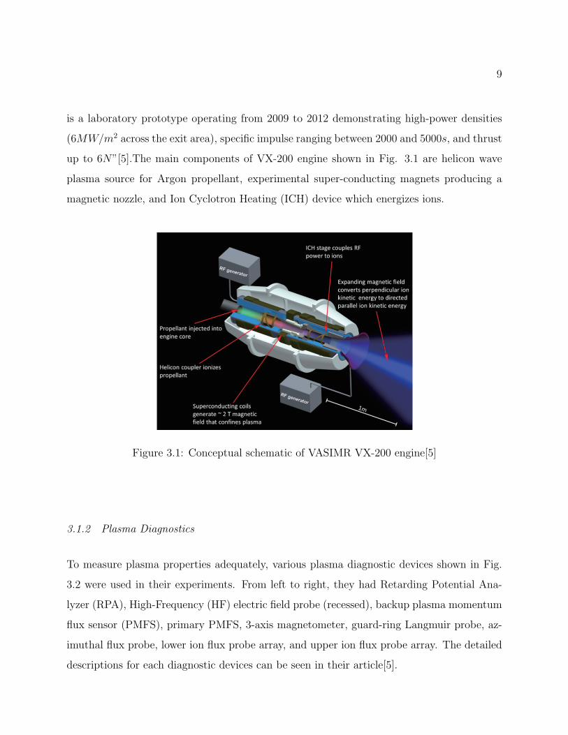
is a laboratory prototype operating from 2009 to 2012 demonstrating high-power densities

(6MW/m2 across the exit area), specific impulse ranging between 2000 and 5000s, and thrust

up to 6N”[5].The main components of VX-200 engine shown in Fig. 3.1 are helicon wave

plasma source for Argon propellant, experimental super-conducting magnets producing a

magnetic nozzle, and Ion Cyclotron Heating (ICH) device which energizes ions.

Figure 3.1: Conceptual schematic of VASIMR VX-200 engine[5]

3.1.2 Plasma Diagnostics

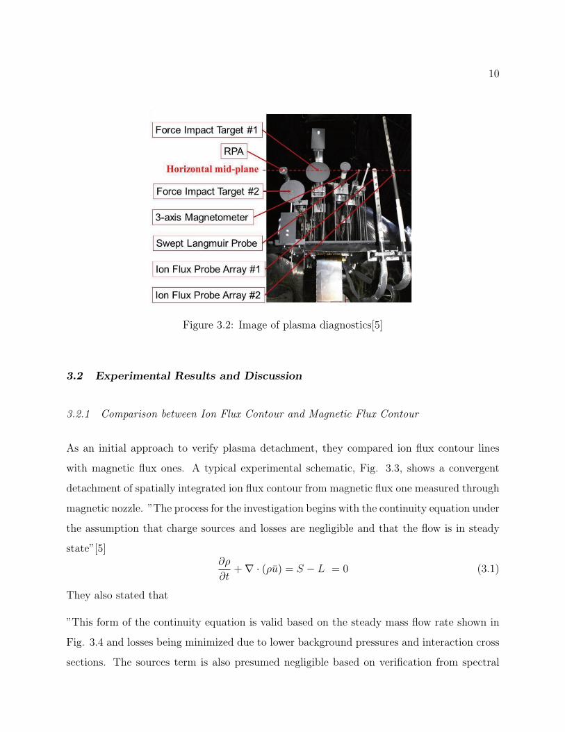
To measure plasma properties adequately, various plasma diagnostic devices shown in Fig.

3.2 were used in their experiments. From left to right, they had Retarding Potential Ana-

lyzer (RPA), High-Frequency (HF) electric field probe (recessed), backup plasma momentum

flux sensor (PMFS), primary PMFS, 3-axis magnetometer, guard-ring Langmuir probe, az-

imuthal flux probe, lower ion flux probe array, and upper ion flux probe array. The detailed

descriptions for each diagnostic devices can be seen in their article[5].

10

Figure 3.2: Image of plasma diagnostics[5]

3.2 Experimental Results and Discussion

3.2.1 Comparison between Ion Flux Contour and Magnetic Flux Contour

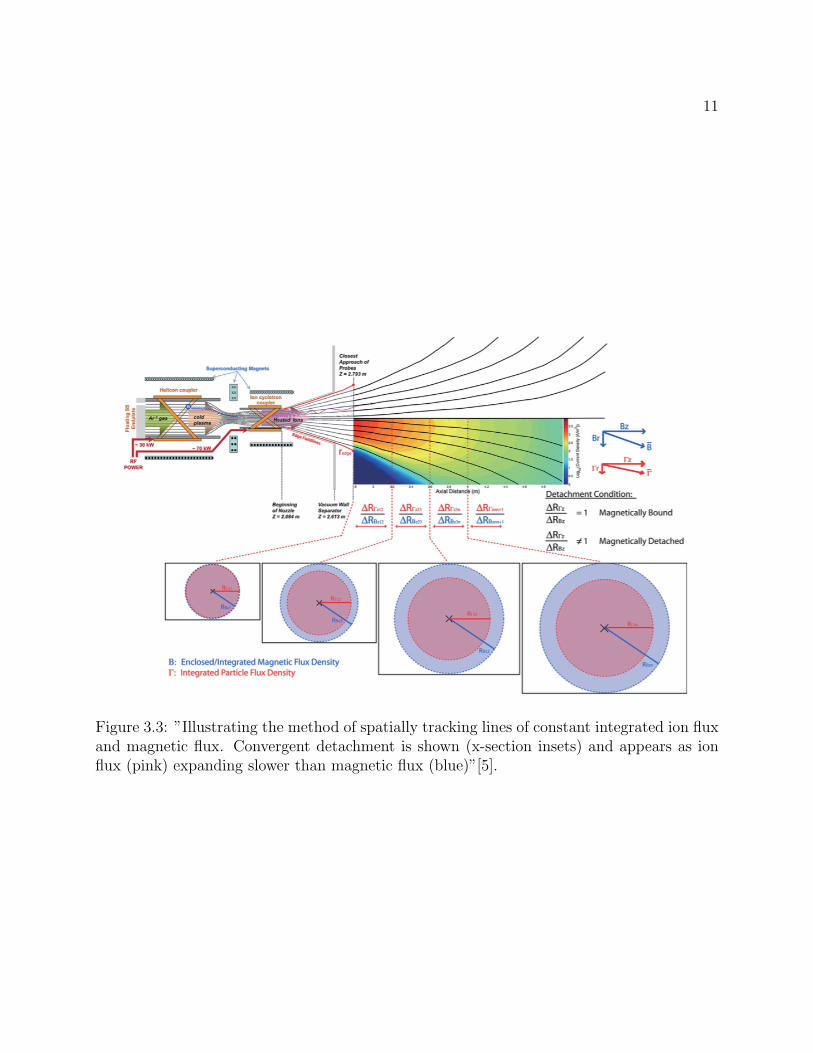
As an initial approach to verify plasma detachment, they compared ion flux contour lines

with magnetic flux ones. A typical experimental schematic, Fig. 3.3, shows a convergent

detachment of spatially integrated ion flux contour from magnetic flux one measured through

magnetic nozzle. ”The process for the investigation begins with the continuity equation under

the assumption that charge sources and losses are negligible and that the flow is in steady

state”[5]∂ρ

∂t+∇ · (ρu) = S − L = 0 (3.1)

They also stated that

”This form of the continuity equation is valid based on the steady mass flow rate shown in

Fig. 3.4 and losses being minimized due to lower background pressures and interaction cross

sections. The sources term is also presumed negligible based on verification from spectral

11

Figure 3.3: ”Illustrating the method of spatially tracking lines of constant integrated ion fluxand magnetic flux. Convergent detachment is shown (x-section insets) and appears as ionflux (pink) expanding slower than magnetic flux (blue)”[5].

12

data of a singly ionized plume, low-ion collision rate, and lack of additional external energy

sources. The continuity equation permits the measurement of the plasma/magnetic flux

expansion without worry of external influences.”[5]

To obtain ion flux contour lines and magnetic flux ones, they numerically solved following

set of operations at each axial locations where radial profile data were taken by Langmuir

probe arrays facing at axial direction.

Γiz (r) = 2π

∫ r

0

Jiz/qrdr (3.2)

fi (r) =Γiz (r)

Γiz (redge)(3.3)

Φz (r) = 2π

∫ r

0

Bzrdr (3.4)

fΦ = Φz (rfi) (3.5)

Eq. 3.2 and 3.3 describe ion flux and ion plume fraction, fi, which are used to map constant

ion flux lines. redge is a geometric projection of the magnetic field from the inner wall shown

in Fig. 3.3. Eq. 3.4 and 3.5 describe the radial magnetic flux integration and magnetic flux

originally enclosing the baseline of an ion plume fraction line. To verify plasma detachment,

they plotted fi and fΦ in Fig. 3.5 as a comparison between constant ion flux lines and

constant magnetic flux ones. While they showed other results in their article for the case

where only helicon plasma source was used, in this paper I particularly focus on results from

the operations using both helicon source and ICH. Note that these equations are slightly

different from theirs shown in their article because I found few issues in their definitions. At

first, they defined magnetic flux fraction by

fΦ (r) =Φz (r)

Φ0z (rfi)(3.6)

However, if they used their definition adequetly, their magnetic flux fraction lines would not

match with their black dashed lines shown in Fig. 3.5. For example, when they mapped

fΦ (r) = 90% line, their fΦ line would indicate 90% of magnetic flux starting from the baseline

13

Figure 3.4: ”Standard shot configuration including uncertainty bounds (dashed lines). Dataanalysis windows for the low- and high-power configurations were taken from 0.4 ‒ 0.5 and0.65 ‒ 0.75 s, respectively. Top: average RF forward power profile. Middle: steady 3600-sccm (~ 107 mg/s) argon flow. Bottom: exhaust region chamber pressure measured byseparate hot cathode ion gauges.”[5]

14

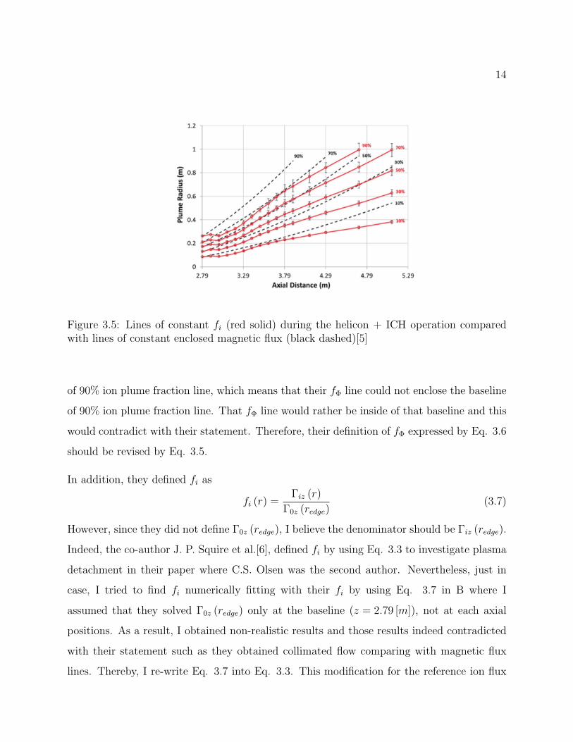
Figure 3.5: Lines of constant fi (red solid) during the helicon + ICH operation comparedwith lines of constant enclosed magnetic flux (black dashed)[5]

of 90% ion plume fraction line, which means that their fΦ line could not enclose the baseline

of 90% ion plume fraction line. That fΦ line would rather be inside of that baseline and this

would contradict with their statement. Therefore, their definition of fΦ expressed by Eq. 3.6

should be revised by Eq. 3.5.

In addition, they defined fi as

fi (r) =Γiz (r)

Γ0z (redge)(3.7)

However, since they did not define Γ0z (redge), I believe the denominator should be Γiz (redge).

Indeed, the co-author J. P. Squire et al.[6], defined fi by using Eq. 3.3 to investigate plasma

detachment in their paper where C.S. Olsen was the second author. Nevertheless, just in

case, I tried to find fi numerically fitting with their fi by using Eq. 3.7 in B where I

assumed that they solved Γ0z (redge) only at the baseline (z = 2.79 [m]), not at each axial

positions. As a result, I obtained non-realistic results and those results indeed contradicted

with their statement such as they obtained collimated flow comparing with magnetic flux

lines. Thereby, I re-write Eq. 3.7 into Eq. 3.3. This modification for the reference ion flux

15

Γ0z (redge) will indeed bring a serious issue to their statement.

From Fig. 3.5, they concluded that the separation between ion plume fraction lines and

magnetic flux lines indicated the separation between ion flux contours and magnetic flux

contours originally enclosing the ion plume fraction lines. However, since they plotted con-

stant fi lines instead of constant Γiz (r) lines, their statement could be valid only when the

denominator Γiz (redge) is constant. For example, when fi = const and the denominator

Γiz (redge) is not constant, the numerator Γiz (r) cannot become constant neither. One possi-

ble case that satisfies this example can be seen in Fig. 3.6. In their experiments, since they

Figure 3.6: Possible shapes of plasma plume and redge

defined redge as a magnetic field line, it does not have to fit with the plasma plume edge line

after leaving the physical inner wall. Thus, Γiz (redge) is not necessarily constant throughout

magnetic nozzle. Consequently, I can state that the deviations of fi lines from magnetic flux

ones did not always indicate the deviations of constant ion flux Γiz (r) lines from magnetic

flux ones. In other words, their first key indication of plasma detachment such as ion flux

contours detached from magnetic flux ones is not necessarily correct.

16

3.2.2 Ion Unmagnetization

As the second key indication of plasma detachment, they compared ion velocity vectors

with magnetic field ones by using RPA data. Contour plots of an ion velocity distribution

function as a function of radial and axial ion velocity with a local magnetic field vector are

shown in Fig. 3.7. They stated that ”If the ions were magnetized much of the distribution

Figure 3.7: Contour maps of the ion velocity distribution function as a function of vr and vzat five radial locations and z = 3.9 [m]. ”The local magnetic field vector is overlain in eachplot (black arrow)”[5]

would be expected to be more preferentially organized near the angle of the magnetic field

vector”[5]. In fact, at the larger radial positions where the field has begun to curve away,

axial component of ion velocity seemed to be more dominant comparing with magnetic

field vector. This result was the proof of ion unmagnetization and became the second key

indication of plasma detachment.

17

3.2.3 Existence of High-frequency Electric Field

As the third key indication, they observed high-frequency electric field, especially around the

plume edge, due to loss of adiabaticity. According to [9], the breakdown of loss of adiabaticity

occurs when the change in Larmor radius becomes comparable with itself.

∆rLirLi

=∆Ωci

Ωci

=νiΩci

|∇B|B

= 1 (3.8)

In their experiments, the breakdown for ions occurred at the green dashed line in Fig. 3.8,

while electrons did not lose their adiabaticity over the entire measurement region. After

Figure 3.8: ”Image summarizing various regions associated with detachment process. Theflow lines (blue) are based on the integrated ion flux fraction and extended out along thelinear region. Lines showing the transition above unity for kinetic and thermal beta aredisplayed for reference (red dashed)”[5]

losing adiabaticity, plasma entered the ion trapping region. In this region, perturbed high-

frequency electric field appeared between unmagnetized ions and magnetized electrons. This

electric field worked as E × B force and that force produced diamagnetic current. Then,

J× B force eventually worked as centrifugal force on ions. In particular, since magnetic field

18

was still strong around the nozzle exit, the centrifugal force was dominant comparing with

electrostatic force; hence ions seemed to be trapped.

On the other hand, as magnetic field was weakened, the fluctuating electrostatic force be-

came dominant and plasma entered the anomalous transport region. In this region, ef-

fective collision rate for interparticle collisions was increased, and then effective resistivity

became anomalous resistivity [5],[56],[10],[11]. In consequence, the tug-of-war between elec-

trostatic force and centrifugal force enabled plasma to transport anomalously across magnetic

field.

Beyond the anomalous transport region, the ions’ trajectories became linear and the fluctu-

ating electric fields were dissipated. However, since electrons were still magnetized, I believe

that anomalous transport and fluctuating electric fields should still exist in the ballistical

detached plasma region. Regarding this point, they mentioned that

”Although not directly observed, anomalous transport may still be occurring in the weak

magnetic field regions beyond the limits of the translation stage. It may be the focus of

future experiments to explore the plume further out in radius during plasma operation at

lower ion energy.” [5]

3.3 Summary of VASIMR VX-200 Research

In summary, they observed three key indications of plasma detachment. At first, they showed

ion detachment from a magnetic flux contour, although it was not necessarily correct. Next,

they indicated ion unmagnetization at larger radial positions. Lastly, they observed the

existence of high-frequency electric field between magnetized electrons and unmagnetized

ions due to loss of adiabaticity.

19

Chapter 4

CANONICAL FIELD THEORY

To investigate the plasma detachment described in section 3, I will apply canonical field

theory formalized by You [1], [2], [3]. In general, interactions between plasma flow and

electromagnetic field produce additional complexities and difficulties like non-ideal effects

seen in MHD theory (e.g., resistive collisions, Hall effect, inertia effect, pressure gradient

and pressure tensor). Around a plasma plume edge, density gradient might produce kinetic

effects which cannot be investigated via fluid regime. To reduce those complexities and cost

for investigations, most of analyses and numerical simulations do not include those realistic

effects.

Whereas, You formalized canonical field theory from the most fundamental point-of-view

using generalized Lagrangian-Hamiltonian formalism for dynamics of single particle, kinetic

and fluid regimes[3]. As one of the biggest advantages of using canonical field theory, it

allows us to consider more fundamental plasma physics including non-ideal and even non-

fluid-regime effects. Moreover, it has one-to-one relationship with MHD theory. For example,

there exist one-to-one relationships between canonical vorticity field Ωσ and magnetic field

B, between canonical force field Σσ and electric field E, and between general enthalpy hσ

and some of plasma energy (e.g., kinetic energy, electrostatic potential energy, and pres-

sure energy). Using these one-to-one relationships, we can simply apply conventional MHD

intuition for canonical field theory.

20

4.1 Governing Equations

In this section, I will introduce governing equations in canonical field theory. Whole detailed

derivations are shown in [3]. First and foremost, let me define canonical momentum Pσ for

certain plasma species σ as

Pσ ≡ nσmσuσ + nσqσAσ (4.1)

General enthalpy is defined as

hσ ≡1

2nσmσu

2σ + nσqσϕ+ Pσ (4.2)

Canonical vorticity field is defined by

Ωσ ≡ ∇× Pσ (4.3)

Canonical force-field is defined by

Σσ ≡ −∇hσ −∂Pσ

∂t(4.4)

From generalized Lagrangian-Hamiltonian formalism, generalized form of Ohm’s law (equa-

tion of motion) can be written as

Σσ +(uσ × Ωσ

)= Rσ (4.5)

where dissipative force Rσ is

Rσ ≡ −∇(1

2ϵσΣ

2σ −

Ω2σ

2µσ

)(4.6)

You[3] explained Eq. 4.6 by stating that ”dissipative forces represent an incomplete conver-

sion of canonical vorticity ”potential” energy Ω2σ

2µσinto canonical force-field ”kinetic” energy

12ϵσΣ

2σ.”

Next, let me derive generalized form of Maxwell’s equations in canonical field theory. First of

all, generalized Faraday’s law can be derived by taking curl of canonical force field Σσ,

∇× Σσ = −∂Ωσ

∂t(4.7)

21

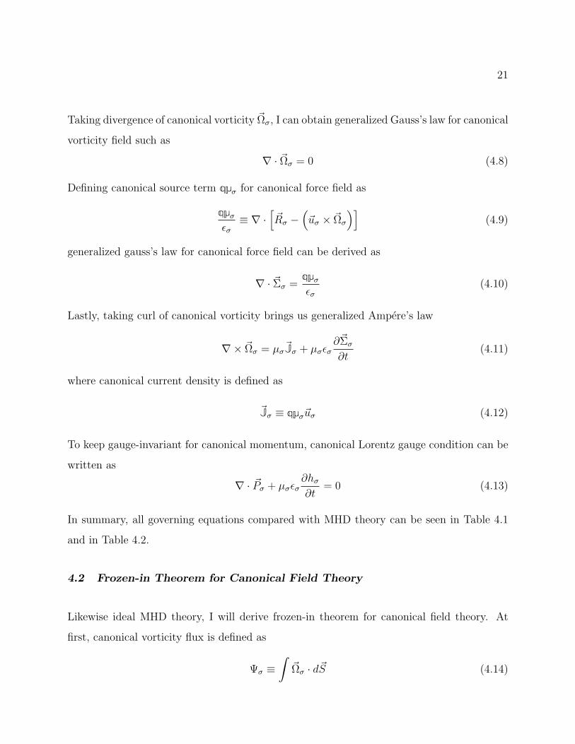
Taking divergence of canonical vorticity Ωσ, I can obtain generalized Gauss’s law for canonical

vorticity field such as

∇ · Ωσ = 0 (4.8)

Defining canonical source term qµσ for canonical force field as

qµσ

ϵσ≡ ∇ ·

[Rσ −

(uσ × Ωσ

)](4.9)

generalized gauss’s law for canonical force field can be derived as

∇ · Σσ =qµσ

ϵσ(4.10)

Lastly, taking curl of canonical vorticity brings us generalized Ampere’s law

∇× Ωσ = µσJσ + µσϵσ∂Σσ

∂t(4.11)

where canonical current density is defined as

Jσ ≡ qµσuσ (4.12)

To keep gauge-invariant for canonical momentum, canonical Lorentz gauge condition can be

written as

∇ · Pσ + µσϵσ∂hσ∂t

= 0 (4.13)

In summary, all governing equations compared with MHD theory can be seen in Table 4.1

and in Table 4.2.

4.2 Frozen-in Theorem for Canonical Field Theory

Likewise ideal MHD theory, I will derive frozen-in theorem for canonical field theory. At

first, canonical vorticity flux is defined as

Ψσ ≡∫

Ωσ · dS (4.14)

22

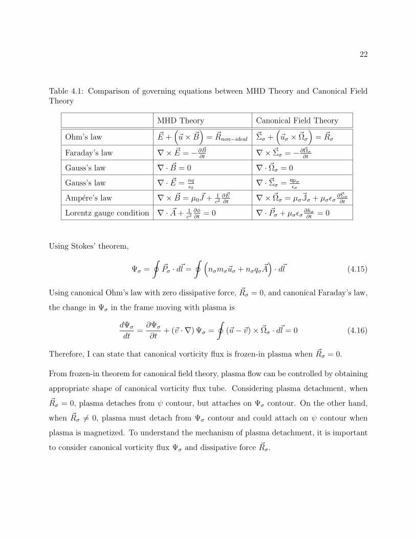
Table 4.1: Comparison of governing equations between MHD Theory and Canonical FieldTheory

MHD Theory Canonical Field Theory

Ohm’s law E +(u× B

)= Rnon−ideal Σσ +

(uσ × Ωσ

)= Rσ

Faraday’s law ∇× E = −∂B∂t

∇× Σσ = −∂Ωσ

∂t

Gauss’s law ∇ · B = 0 ∇ · Ωσ = 0

Gauss’s law ∇ · E = nqϵ0

∇ · Σσ = qµσ

ϵσ

Ampere’s law ∇× B = µ0J + 1c2

∂E∂t

∇× Ωσ = µσJσ + µσϵσ∂Σσ

∂t

Lorentz gauge condition ∇ · A+ 1c2

∂ϕ∂t

= 0 ∇ · Pσ + µσϵσ∂hσ

∂t= 0

Using Stokes’ theorem,

Ψσ =

∮Pσ · dl =

∮ (nσmσuσ + nσqσA

)· dl (4.15)

Using canonical Ohm’s law with zero dissipative force, Rσ = 0, and canonical Faraday’s law,

the change in Ψσ in the frame moving with plasma is

dΨσ

dt=∂Ψσ

∂t+ (v · ∇)Ψσ =

∮(u− v)× Ωσ · dl = 0 (4.16)

Therefore, I can state that canonical vorticity flux is frozen-in plasma when Rσ = 0.

From frozen-in theorem for canonical field theory, plasma flow can be controlled by obtaining

appropriate shape of canonical vorticity flux tube. Considering plasma detachment, when

Rσ = 0, plasma detaches from ψ contour, but attaches on Ψσ contour. On the other hand,

when Rσ = 0, plasma must detach from Ψσ contour and could attach on ψ contour when

plasma is magnetized. To understand the mechanism of plasma detachment, it is important

to consider canonical vorticity flux Ψσ and dissipative force Rσ.

23

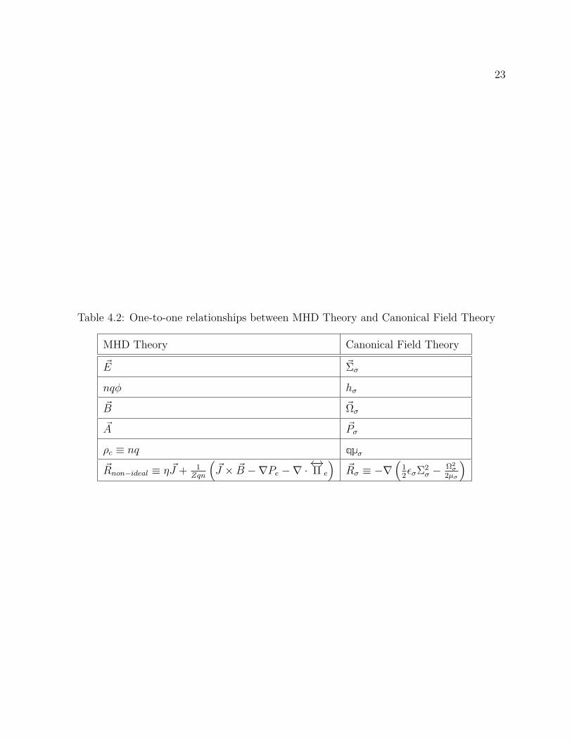
Table 4.2: One-to-one relationships between MHD Theory and Canonical Field Theory

MHD Theory Canonical Field Theory

E Σσ

nqϕ hσ

B Ωσ

A Pσ

ρc ≡ nq qµσ

Rnon−ideal ≡ ηJ + 1Zqn

(J × B −∇Pe −∇ ·

←→Π e

)Rσ ≡ −∇

(12ϵσΣ

2σ −

Ω2σ

2µσ

)

24

Chapter 5

ANALYSIS OF PLASMA DETACHMENT VIA CANONICALFIELD THEORY

From Eq. 4.15, there are three key steps to map canonical vorticity flux Ψσ contour: finding

vector potential A, finding number density profile nσ, and finding velocity profile uσ. In

this section, I will present analytical fits with experimental data shown in section 3, and

investigate the mechanism of plasma detachment via canonical field theory.

5.1 Constant Ion Flux Contour

5.1.1 Magnetic Field Configuration

In the experiments, the magnetic field is produced from experimental superconducting mag-

nets. However, due to less information about those magnets (e.g., location, width, radius,

and current carried) in their article, let me assume that an ideal single current loop produces

magnetic field

Aθ =µ0

4π

4Ia√a2 + r2 + z2 + 2ar

[(2− k2)K (k)− 2E (k)

k2

](5.1)

where a is a radius of a circular current loop carrying current I and the argument k of the

elliptic integral is

k2 =4ar

a2 + r2 + z2 + 2ar(5.2)

Taking curl of A, I can obtain the following similar enough magnetic field configuration

shown in Fig. 5.1 and Fig. 5.2. Note that there are three different experimental results in

Fig. 5.1; one is for vacuum case, another one is for helicon plasma source with ICH case, the

25

Figure 5.1: Comparison for the strength of magnetic field on z-axis for vacuum case (black),helicon only case (blue), and helicon + ICH case (red) in experiments and my analytical one(green)[5]

other one is for helicon plasma source without ICH case. Olsen et al., mentioned that these

three experimental results were mostly overlapped, and the largest difference was only 2%.

5.1.2 Number Density Profile

Number density profile can be derived from current density profile measured by Langmuir

probe arrays such as

jiz (r, z) = e−12ni (r, z) qics (z) (5.3)

where I assumed quasineutral plasma (ne = ni). Bohm velocity cs (z) can be derived from

current density and number density data measured on z-axis where I assumed radially uni-

form Bohm velocity because of less information about its radial profile.

cs (z) =jiz (0, z)

e−12ni (0, z) qi

(5.4)

26

Figure 5.2: Comparison for experimental magnetic flux lines (black dashed), experimentalmagnetic flux fraction fi lines (red) and my analytical magnetic flux (blue dashed)[5]

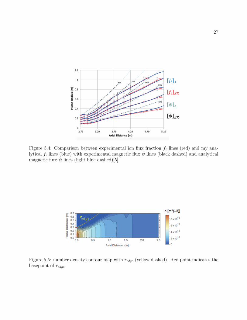
Regarding radial current density profile, I assumed Gaussian distribution jiz (r, z) ∝ e−arb

and numerically solved for ion plume fraction lines fi fitting with experimental ones shown

in Fig. 5.4. From Fig. 5.4, I can confirm that my analytical constant ion plume fraction fi

Figure 5.3: Axial ion current density contour map

lines (blue) seem to match with measured ones (red).

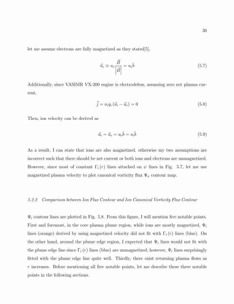
Plotting number density contour map with redge line (yellow dashed line) in Fig. 5.5, I can

see that redge at the beginning is indeed placed inside the plume edge like I expected in

Fig. 3.6. From this result, I can state that Γi (redge) is not necessarily constant at each

27

Figure 5.4: Comparison between experimental ion flux fraction fi lines (red) and my ana-lytical fi lines (blue) with experimental magnetic flux ψ lines (black dashed) and analyticalmagnetic flux ψ lines (light blue dashed)[5]

Figure 5.5: number density contour map with redge (yellow dashed). Red point indicates thebasepoint of redge

28

axial position. In fact, calculating Γi (redge), I can show non-constant Γi (redge) in Fig. 5.6.

As a result, I can conclude that their first key indication, ”ion flux contour detached from

Figure 5.6: number density contour map with redge (yellow dashed). Red point indicates thebasepoint of redge

magnetic flux contour” was incorrect. Plotting actual constant ion flux contour lines in Fig.

5.7, I can see that most of constant ion flux contour lines did not actually separate from

magnetic flux contour ones.

On the other hand, my analytical constant ion flux Γi (r) lines are consistent with their

second key indication. At z = 1.2 in Fig. 5.7 (at z = 3.9 in their experiments), Γi (r) lines

start to separate and be collimated at larger radial positions. This result is consistent with

their second indicator such that ”ions became unmagnetized and collimated as r increases.”

As another possible counter-argument to my analysis, it can be stated that Γi (r) lines might

not be true constant ion flux lines because they used informal definition for ion flux. In

general, ion flux should be defined as

Γitrue ≡∫niui · dS (5.5)

Whereas, in their article, ion flux was defined by using current density obtained from Lang-

29

Figure 5.7: ni contour map with constant ion flux Γi (r) lines (blue solid), constant magneticflux ψ lines (light blue dashed), and redge (yellow dashed)

muir probes

Γiex =

∫e−

12n∞cs · dS (5.6)

This informal definition would bring inadequate plots for ion flux contour lines. However,

since my analytical Γi (r) lines are consistent with their second evidence based on RPA data,

at least I can state that my Γi (r) lines are approximately equal to the true ones, Γiex ≃ Γitrue,

except for the plume edge region.

5.2 Canonical Vorticity Flux Contour

5.2.1 Velocity Profile

To understand plasma detachment around the plume edge region, we need to plot canonical

vorticity flux Ψσ contour lines. The last step to map Ψσ contours, I need to find velocity

profile. Unfortunately, since we have less information about the radial profile of ion velocity,

30

let me assume electrons are fully magnetized as they stated[5],

ue ≡ ueB∣∣∣B∣∣∣ = ueb (5.7)

Additionally, since VASIMR VX-200 engine is electrodeless, assuming zero net plasma cur-

rent,

j = niqi (ui − ue) = 0 (5.8)

Then, ion velocity can be derived as

ui = ue = ueb = uib (5.9)

As a result, I can state that ions are also magnetized, otherwise my two assumptions are

incorrect such that there should be net current or both ions and electrons are unmagnetized.

However, since most of constant Γi (r) lines attached on ψ lines in Fig. 5.7, let me use

magnetized plasma velocity to plot canonical vorticity flux Ψσ contour map.

5.2.2 Comparison between Ion Flux Contour and Ion Canonical Vorticity Flux Contour

Ψi contour lines are plotted in Fig. 5.8. From this figure, I will mention five notable points.

First and foremost, in the core plasma plume region, while ions are mostly magnetized, Ψi

lines (orange) derived by using magnetized velocity did not fit with Γi (r) lines (blue). On

the other hand, around the plume edge region, I expected that Ψi lines would not fit with

the plume edge line since Γi (r) lines (blue) are unmagnetized; however, Ψi lines surprisingly

fitted with the plume edge line quite well. Thirdly, there exist returning plasma flows as

r increases. Before mentioning all five notable points, let me describe these three notable

points in the following sections.

31

Figure 5.8: ni contour map with constant canonical vorticity flux Ψi lines (orange), constantion flux Γi (r) lines (blue), constant magnetic flux ψ lines (light blue dashed), and redge(yellow dashed)

5.2.3 Dissipative Term Rσ makes Plasma Detach from Canonical Vorticity Flux Con-

tour

As for the first notable point, I can simply explain by using non-zero dissipative force, Rσ = 0.

As I had already mentioned in section 4, when Rσ = 0, plasma can detach from Ψσ contour.

Therefore, in the core plasma plume region, non-zero dissipative force, Rσ = 0, makes plasma

detach from Ψσ lines (orange) and attach on ψ lines (light blue dashed). Thereby both ions

and electrons can be magnetized.

In contrast, Rσ = 0 force enables plasma to attach on Ψσ contour lines around the plume

edge region. In that region, since nσ → 0, I can write Ωσ → 0 and Σσ → 0. Hence, even if

we used inaccurate velocity profile to plot Ψσ, like magnetized velocity, canonical vorticity

flux and dissipative term would become Ψσ → cst and Rσ → 0. As a result, I can state my

analytical Ψi lines are approximately equal to the true ones that should be derived by using

the true velocity profile around the plume edge region, and exactly same at the plume edge

due to Rσ = 0.

32

5.2.4 Returning Plasma Flow

The existence of returning plasma flow is guaranteed by Gauss’s law for canonical vorticity

field such as ∇ · Ωσ = 0 like a closed loop of magnetic field. However, unlike magnetic field,

since Ωσ is defined by using number density nσ, all returning paths should be enclosed by a

plasma plume edge. Mathematically, these returning points appear when ∂Ψσ

∂z= 0.

∂Ψσ

∂z=

∮∂Pσ

∂z· dl =

∮ [∂nσ

∂z

(mσuσ + qσA

)+ nσ

(mσ

∂uσ∂z

+ qσ∂A

∂z

)]· dl (5.10)

In general, nσ → 0 and ∂nσ

∂z→ 0 around the plume edge region. Therefore, I can infer that

returning points will appear around the plume edge region.

5.2.5 Additional Notable Points

Another notable point from Fig. 5.8 is that ion flux Γi (r) lines around the nozzle exit

separate from Ψσ lines and diverge to infinity. In my opinion, since Olsen et al., measured

the current density by using −z directed Langmuir probes, they could not measure returning

plasma flow appropriately. For this reason, ion flux Γi (r) lines around the nozzle exit seem

to diverge to infinity.

Regarding the high-frequency electric field, I can explain the existence and dissipation of

this electric field by considering canonical vorticity flux for ions Ψi and for electrons Ψe. In

the core plume region, since both ions and electrons are magnetized, it is difficult to observe

electric field. In fact, the author stated that the strength of electric field was larger as r

increases. Around the plume edge region, since Rσ ≃ 0, both ions and electrons try to re-

attach on their own canonical vorticity flux Ψσ contours. Then, when constant Ψi lines do

not match with constant Ψe lines, electric field appears, vice versa. Considering canonical

vorticity flux for each species, the biggest difference can be seen in their inertia terms.

Ψi =

∮ (nimiui + niqiA

)· dl (5.11)

33

Ψe =

∮ (nemeue + neqeA

)· dl (5.12)

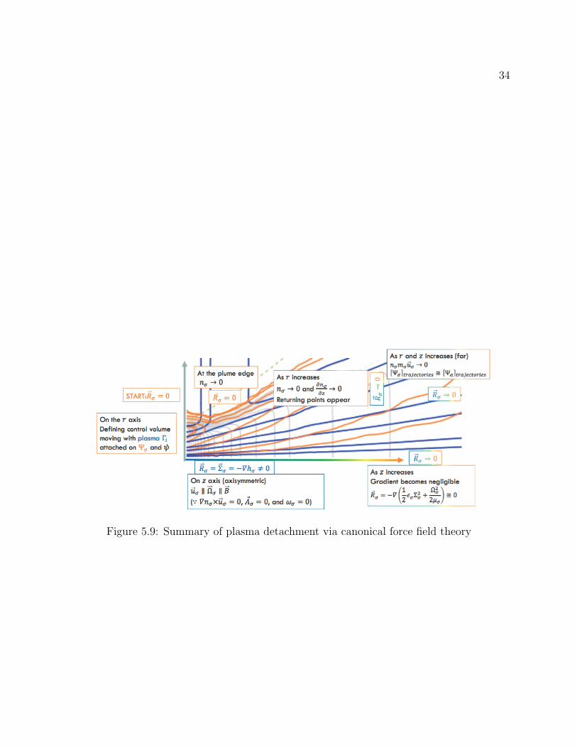
Around the nozzle exit, since the inertia effects for each species are not negligible, constant

Ψi lines deviate from constant Ψe lines. In contrast, since number density becomes much

smaller at the far downstream region than that around the nozzle exit, those inertia effects

can become negligible. As a result, high-frequency electric field can be dissipated. This

explanation is consistent with their third key indication such that they observed strong

perturbed electric field around the plume edge and it dissipated as z increases.

5.3 Summary of Analysis

I confirmed that my analytical results via canonical field theory are consistent with two of

three key indications observed in VASIMR experimental research. At first, their first key

indication becomes incorrect now because Γi (redge) is actually not constant, and constant ion

flux lines did not actually separate from magnetic flux ones. Secondly, my analytical ion flux

Γi (r) lines showed the consistent result with their second key indication, namely analytical

Γi (r) lines are also deviated and collimated at larger radial positions. Lastly, while electrons

are neither fully magnetized around the plume edge region because of Rσ ≃ 0, I can explain

the existence of high-frequency electric field by considering deviations between Ψi lines and

Ψe lines. Also, the dissipation of the electric field at larger axial locations can be explained

by matching of Ψi lines and Ψe ones.

The transitions of dissipative force and the mechanism of plasma detachment through mag-

netic nozzle are summarized in Fig. 5.9.

34

Figure 5.9: Summary of plasma detachment via canonical force field theory

35

Chapter 6

SUMMARY

In this paper, I have investigated the mechanism of plasma detachment through magnetic

nozzle via canonical field theory. As one of the most recent experimental proofs, Olsen et

al[5]., observed and investigated plasma detachment through magnetic nozzle in VASIMR

VX-200 engine. In their article, they observed three key indications of plasma detachment;

constant ion flux lines deviated from constant magnetic flux ones; ions became unmagnetized

at larger radial locations; high-frequency electric field appeared and dissipated as z increases.

However, since I found some issues in their definitions, in particular their calculations for the

reference ion flux Γi (redge), their first key indication becomes incorrect now. After solving

for numerical fits with their experimental results, I found that constant ion flux Γi (r) lines

did not actually separate from constant magnetic flux ones. Whereas, my analytical results

are consistent with the other two key indications. My analytical constant ion flux Γi (r) lines

are collimated and deviated from magnetic flux ones as r increases. In addition, their third

key indication can be explained by considering the separation between canonical vorticity

flux contours for each ions and electrons.

To explain the mechanism of plasma detachment, I utilized frozen-in theorem in canonical

field theory likewise ideal MHD theory; canonical vorticity flux is frozen-in plasma when

dissipative force Rσ = 0. At the beginning, plasma detached from canonical vorticity flux

Ψσ contours due to non-zero dissipative force Rσ = 0 and could attache on rather magnetic

flux lines. However, since number density nσ decreases as r increases, dissipative force is

getting close to zero. As a result, Rσ ≃ 0 force makes plasma re-attach on canonical vorticity

flux Ψσ contours. Also, at the quite far downstream region from magnetic nozzle, since most

36

of plasma parameters become approximately uniform, Rσ ≡ −∇(

12ϵσΣ

2σ −

Ω2σ

2µσ

)≃ 0 and

plasma try to re-attach on Ψσ contour.

Another notable point for Ψσ contour is the existence of returning plasma flow. Likewise

magnetic field, since canonical vorticity field Ωσ also satisfies Gauss’s law, Ωσ should have a

closed loop trajectory. On the other hand, unlike magnetic field, since Ωσ is defined by using

nσ, all returning paths should be enclosed by a plasma plume edge. Therefore, as nσ and

axial gradient of number density ∂nσ

∂zdecrease and get close to zero at larger radial positions,

plasma should re-attach on Ψσ lines and eventually returns to the nozzle.

Meanwhile, constant Ψi lines do not have to match with constant Ψe lines even around

the plume edge region. In particular, around the nozzle exit, since inertia effects cannot

be negligible, the deviations of each Ψσ trajectories generate high-frequency electric field

around the plume edge region. At the far downstream region, by contrast, since nσ decreases

through diverging magnetic nozzle, inertia effects become negligible and Ψσ trajectories for

each species match with one another. Eventually, electric field between ions and electrons

dissipates at the far downstream region. This is consistent with their third key indication

observed in the VASIMR experiment.

In conclusion, canonical field theory can explain the mechanism of plasma detachment by

considering canonical vorticity flux contour and a transition of dissipative force. The analyses

via canonical field theory are mostly consistent with VASIMR VX-200 experimental results.

To verify the existence of the returning plasma flow, I suggest to use Mach probes instead

of using Langmuir probes. Also, it is necessary to plot true canonical vorticity flux contour

by using true velocity profile obtained from Mach probes or RPA arrays. For more practical

purposes, it is also quite important to investigate the dynamics of canonical vorticity flux

tube for analyzing plasma detachment and a formation of returning plasma flow through a

plasma jet.

37

Appendix A

FROZEN-IN THEOREM

Frozen-in theorem in ideal MHD theory is derived based on

dψ

dt= 0 (A.1)

Using Eq. 2.1,dψ

dt=

∫dB

dt· dS +

∫B · d∆S

dt(A.2)

The first term becomes∫dB

dt· dS = lim

δt→0

∫B (t+ δt)− B (t)

δt· dS =

∫∂B (t)

∂t· dS (A.3)

Using Faraday’s law and Ohm’s law,∫∂B (t)

∂t· dS =

∫∇×

(u× B

)· dS (A.4)

Using Stokes’ theorem, ∫∇×

(u× B

)· dS =

∮ (u× B

)· dl (A.5)

The second term is ∫B · d∆S

dt=

∫B · udt×∆l

dt=

∫B ·(u×∆l

)(A.6)

From Eq. A.5 and A.6, these two terms are cancelled out one another by considering triple

scalar product. Therefore, I can derived Eq. A.1.

38

Appendix B

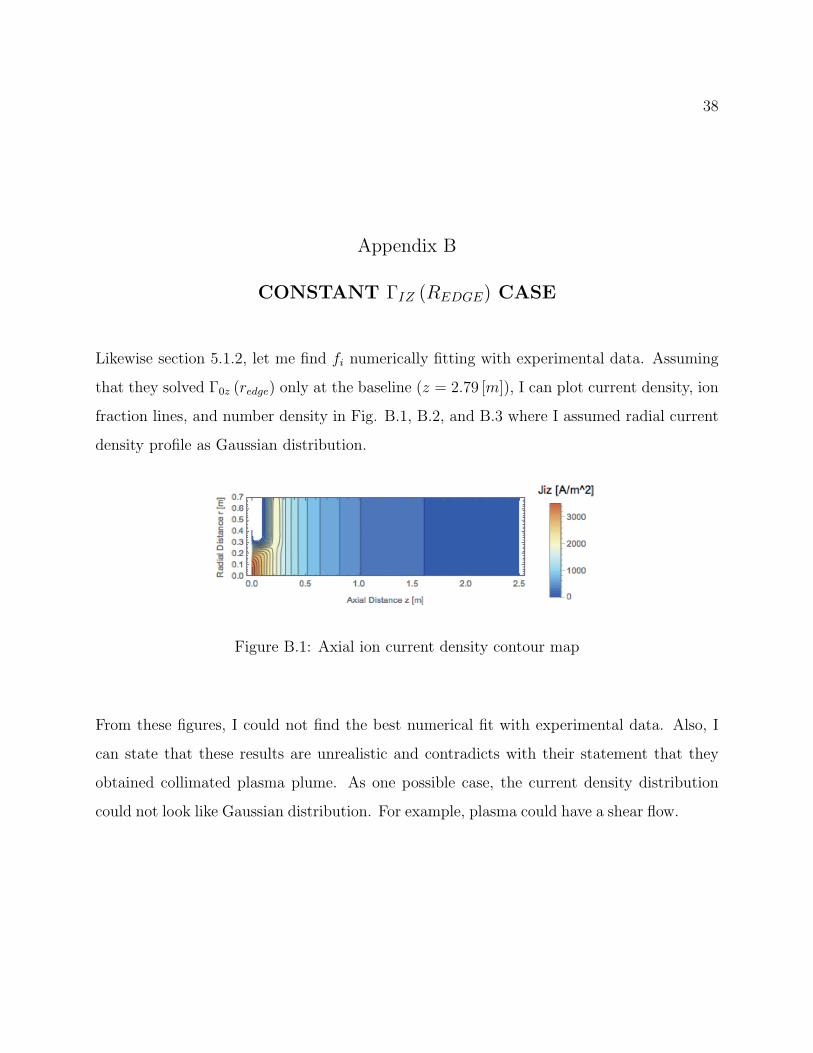
CONSTANT ΓIZ (REDGE) CASE

Likewise section 5.1.2, let me find fi numerically fitting with experimental data. Assuming

that they solved Γ0z (redge) only at the baseline (z = 2.79 [m]), I can plot current density, ion

fraction lines, and number density in Fig. B.1, B.2, and B.3 where I assumed radial current

density profile as Gaussian distribution.

Figure B.1: Axial ion current density contour map

From these figures, I could not find the best numerical fit with experimental data. Also, I

can state that these results are unrealistic and contradicts with their statement that they

obtained collimated plasma plume. As one possible case, the current density distribution

could not look like Gaussian distribution. For example, plasma could have a shear flow.

39

Figure B.2: Comparison between experimental ion flux fraction fi lines (red) and my ana-lytical fi lines (blue) with experimental magnetic flux ψ lines (black dashed) and analyticalmagnetic flux ψ lines (light blue dashed)[5]

Figure B.3: number density contour map with redge (yellow dashed). Red point indicates thebasepoint of redge

40

BIBLIOGRAPHY

[1] S. You, ”The Transport of Relative Canonical Helicity,” Physics of Plasma, vol. 19,Sep. 2012, doi: 10.1063/1.4752215

[2] S. You, ”A Two-fluid Helicity Transport Model for Flux-rope Merging,” Plasma Physicsand Controlled Fusion, vol. 56, Mar. 2014, doi: 10.1088/0741-3335/56/6/064007

[3] S. You, ”A Field Theory Approach to the Evolution of Canonical Helicity and Energy,”Physics of Plasma, vol. 23, Jul. 2016, doi: 10.1063/1.4956465

[4] E. S. Lavine and S. You, ”The Topology of Canonical Flux Tubes in Flared Jet Ge-ometry,” The Astrophysical Journal, 835:89 (pp18), Jan. 2017, doi: 10.3847/1538-4357/835/1/89

[5] C.S. Olsen et al., ”Investigation of Plasma Detachment From a Magnetic Nozzle inthe Plume of the VX-200 Magnetoplasma Thruster,” IEEE Transactions on PlasmaScience, vol. 43(1), Jan. 2015.

[6] J. P. Squire et al., ”VASIMR VX-200 Operation at 200 kW and Plume Measurements:Future Plans and an ISS EP Test Platform,” The 32nd International Electric Propul-sion Conference, 2011

[7] F.R. Chang Diaz, ”An Overview of the VASIMR Engine: High Power Space Propulsionwith RF Plasma Generation and Heating,” American Institute of Physics, ConferenceProceeding 595, 2001.

[8] F. Richard, ”Plasma Physics: an Introduction by Richard Fitzpatrick,” ContemporaryPhysics, vol. 57(4), p.606, doi: 10.1080/00107514.2016.1217047

[9] M. D. Carter et al., ”Radio Frequency Plasma Applications for Space Propulsion,” Int.Conf. on Electromagnetics in Advanced Applications, 1999

[10] E. B. Hooper, ”Plasma Detachment from a Magnetic Nozzle,” Journal of Propulsionand Power, vol. 9(5), Sep. 1993

[11] N. Brenning, T. Hurtig, and M. A. Raadu,“Conditions for plasmoid penetration acrossabrupt magnetic barriers,” Phys. Plasmas, vol. 12, no. 1, pp. 012309-1 ‒ 012309-10,2005

[12] C. K. Chu., ”Magnetohydrodynamic Nozzle Flow with Three Transitions,” Physics ofFluids, vol. 5(5), May. 1962., doi: 10.1063/1.1706656.

41

[13] S. A. Andersen et al., ”Continuous Supersonic PlasmaWind Tunnel,” Physics of Fluids,vol. 12, 1969., doi: 10.1063/1.1692519

[14] D. R. Otis., ”Computation and Measurement of Hall Potentials and Flow-field Pertur-bations in Magnetogasydynamic Flow of an Axisymmetric Free Jet,” Journal of FluidMechanics, vol. 24(1), pp.41-63, Feb. 1965., doi: 10.1017/S0022112066000508

[15] K. Kuriki and O. Okada., ”Experimental Study of a Plasma Flow in a Magnetic Noz-zle,” Physics of Fluids, vol 13(9), pp.2262-2269, Sep. 1970., doi: 10.1063/1.1693232

[16] N. Gohda., ”Interaction between a Shock-Heated Plasma and a Nozzle-Shaped Mag-netic Field,” Journal of the Physical Society of Japan, vol 46(4), Apr. 1979

[17] T. Kammash and M. Lee., ”High-Thrust-High-Specific Impulse Gasdynamic FusionPropulsion System,” Journal of Propulsion and Power, vol. 13(3), May. 1997.

[18] R. P. Hoyt et al., ”Magnetic Nozzle Design for Coaxial Plasma Accelerators,” IEEETransactions on Plasma Science, vol. 23(3), Jun. 1995.

[19] Y. D. Zhugzhada and V. M. Nakariakov., ”Latent Heating of Coronal Loops,” SolarPhysics, vol. 175(1), pp.107-121, Sep. 1997

[20] K. F. Schoenberg et al., ”Magnetohydrodyanmic Flow Physics of Magnetically Noz-zled Plasma Accelerators with Applications to Advanced Manufacturing,” Physics ofPlasmas, vol. 5(5), May. 1998, doi: 10.1063/1.872880

[21] D.C. Black et al., ”Two-dimensional Magnetic Field Evolution Measurements andPlasma Flow Speed Estimates from the Coaxial Thruster Experiment,” Physics ofPlasmas, vol. 1, May. 1994, doi: 10.1063/1.870503

[22] D.C. Black, R. M. Mayo, and R. W. Caress., ”Direct Magnetic Field Measurement ofFlow Dynamics in a Magnetize Coaxial Accelerator Channels,” Physics of Plasmas,vol. 4, May. 1997, doi: 10.1063/1.872415

[23] N.F. Roderick et al., ”Hydro magnetic Rayleigh-Taylor instability in high-velocity gas-puff implosions,” Physics of Plasma, vol.5 (5), May. 1998

[24] H. Nakashima et al., ”Use of an Ignition Facility for Fusion Propulsion Experiments,”Fusion Engineering and Design, vol. 44, 1999

[25] R. A. Gerwin, ”Integrity of the Plasma Magnetic Nozzle,” 2010 Abstracts IEEE Inter-national Conference on Plasma Science, 2010, doi:10.1109/PLASMA.2010.5534049

[26] A.V. Arefiev, and B.N. Breizman., ”Collisionless Plasma Expansion into Vacuum:Two New Twists on an Old Problem,” Physics of Plasmas, vol. 16, Apr. 2009, doi:10.1063/1.3118625

42

[27] A.V. Arefiev and B.N. Breizman, ”Ambipolar Acceleration of Ions in a Magnetic Noz-zle,” Physics of Plasma, vol. 15, Apr. 2008, doi: 10.1063/1.2907786

[28] A.V. Arefiev and B.N. Breizman, ”Theoretical Components of the VASIMR PlasmaPropulsion Concept,” Physics of Plasma, vol. 11(5) May. 2004

[29] A. V. Arefiev and B. N. Breizman., ”Magnetohydrodynamic Scenario of PlasmaDetachment in a Magnetic Nozzle,” Physics of Plasmas, vol. 12, Mar. 2005, doi:10.1064/1.1875632

[30] P. G. Mikelides, P. J. Turchi, and N. F. Roderick., ”Applied-Field Magnetoplasmady-namic Thrusters, Part1: Numerical Simulations Using the MACH2 Code,” Journal ofPropulsion and Power, vol. 16(5), Sep. 2000

[31] I.G. Mikellides et al., ”Design of a Fusion Propulsion System-Part 2: Numerical Simu-lation of Magnetic Nozzle Flows,” Journal of Propulsion and Power, vol. 18(1), pp.152-158, Jan-Feb. 2002

[32] M.Inutake et al., ”Transonic Plasma Flow Passing Through a Magnetic Mirror,” Trans-action of Fusion Science and Technology, vol. 51, Feb. 2007

[33] M.Inutake et al., ”Magnetic-Laval-Nozzle Effect on a Magneto-Plasma-Dynamic Arc-jet,” American Institute of Physics, Conference Proceeding 669, 2003

[34] M.Inutake et al., ”Production of a High-Mach-Number Plasma Flow for an AdvancedPlasma Space Thruster,” Plasma Science and Technology, vol. 6(6), Dec. 2004

[35] M.Inutake et al., ”Improvements of Flow Characteristics for an Advanced PlasmaThruster,” Transactions of Fusion Science and Technology, vol. 27, Jan. 2005

[36] Y. Kajimura, R. Kawabuchi, and H. Nakashima, ”Control Techniques of Thrust Vectorfor Magnetic Nozzle in Laser Fusin Rocket,” Fusion Engineering and Design, vol. 81,2006

[37] Y. Kajimura et al., ”Numerical Simulation of Fusion Plasma Behavior in a MagneticNozzle for Laser Fusion Rocket,” Transactions of Fusion Science and Technology, vol.51, Feb. 2007

[38] Y. Kajimura et al., ”Numerical Simulation of Plasma Behavior in a Magnetic Nozzleof a Laser-plasma Driven Nuclear Electric Propulsion System,” American Institute ofPhysics, Conference Proceeding 1084, 2009

[39] J. Gilland et al., ”Multi-Megawatt MPD Plasma Source Operation and Modeling forFusing Propulsion Simulations,” American Institute of Physics, Conference Proceeding699, 2004

[40] J. Gilland, P. Mikellides, and D. Marriott, ”Energy Deposition via Magnetoplasma-

43

dynamic Acceleration: I. Experiment,” Plasma Sources Science Technology, vol. 18,2009, doi: 10.1088/0963-0252/18/1/015001

[41] H. Tobari et al., ”Characteristics of Electromagnetically Accelerated Plasma Flow inan Externally Applied Magnetic Field,” Physics of Plasmas, vol. 14, Sep. 2007, doi:10.1063/1.2773701

[42] G.S. Choi et al., ”Development of Two Propulsion Systems with Helicon Plasma,”Transaction of Fusion Science and Technology, vol. 51, Feb. 2007

[43] J. J. Brainerd and A. Reisz., ”Electrodeless Experimental Thruster,” American Insti-tute of Physics, Conference Proceeding 1103, 2009

[44] R. Winglee et al., ”Simulation and Laboratory Validation of Magnetic Nozzle Effectsfor the High Power Helicon Thruster,” Physics of Plasmas, vol. 14, Jun. 2007, doi:10.1063/1.2734184

[45] D.G. Chavers et al., ”Momentum and Heat Flux Measurements Using an Impact Targetin Flowing Plasma,” Journal of Propulsion and Power, vol. 22(3) May-Jun. 2006

[46] A. Ando et al., ”ICRF Heating and Plasma Acceleration with an Open Magnetic Fieldfor the Advanced Space Thruster,” Transactions of Fusion Science and Technology,vol. 51, Feb. 2007

[47] G. Vecchi et al., ”A Simulation Approach for ICRF Plasma Thruster Antennas,” Amer-ican Institute of Physics, Conference Proceeding 787, 2005

[48] P.F. Schmit and N.J. Fisch, ”Magnetic Detachment and Plume Control in EscapingMagnetized Plasma,” Journal of Plasma Physics, vol. 75(3), pp. 359-371, Nov. 2008,doi: 10.1017/S0022377808007666

[49] F. N. Gest et al., “Ion Detachment in the Helicon Double-Layer Thruster ExhaustBeam,” Journal of Propulsion and Power, vol. 22 (1) Feb. 2006

[50] R. Kawabuchi et al., ”Numerical Simulation of Plasma Detachment from a MagneticNozzle by using Fully Particle-In-Cell Code,” Journal of Physics, Conference Series112, 2008, doi: 10.1088/1742-6596/112/4/042082

[51] B.N. Breizman, M.R. Tushentsov, and A.V. Arefiev, ”Magnetic Nozzle and PlasmaDetachment Model for a Steady-state Flow,” Physics of Plasmas, vol. 15, Apr. 2008,doi: 10.1063/1.2903844

[52] M.D. West, C. Charles, and R.W. Boswell, ”Testing a Helicon Double Layer ThrusterImmersed in a Space-Simulation Chamber,” Journal of Propulsion and Power, vol. 24(1), Jan-Feb. 2008, doi: 10.2514/1.31414

[53] C.A. Deline et al., ”Plume Detachment from a Magnetic Nozzle,” Physics of Plasmas,vol. 16, Mar. 2009, doi: 10.1063/1.3080206

44

[54] T. Andreussi and F. Pegoraro., ”Magnetized Plasma Flows and Magnetoplasmady-namic Thrusters,” Physics of Plasmas, vol. 17, Jun. 2010, doi:10.1063/1.3447876

[55] E. Ahedo and J. Navarro-Cavalle., ”Helicon Thruster Plasma Modeling: Two-dimensional Fluid-dynamics and Propulsive Performances,” Physics of Plasmas, vol.20, Apr. 2013, doi: 10.1063/1.4798409

[56] E. Ahedo and M. Merino., ”Two-dimensional Supersonic Plasma Acceleration in aMagnetic Nozzle,” Physics of Plasmas, vol. 17, Jul. 2010, doi: 10.1063/1.3442736

[57] E. Ahedo and M. Merino., ”On Plasma Detachment in Propulsive Magnetic Nozzle,”Physics of Plasmas, vol. 18, May. 2011, doi: 10.1063/1.3589268

[58] E. Ahedo and M. Merino., ”Two-dimensional Plasma Expansion in a Magnetic Noz-zle: Separation due to Electron Inertia,” Physics of Plasmas, vol. 19, Aug. 2012, doi:10.1063/1.4739791

[59] K. Takahashi, C. Charles, and R. W. Boswell., ”Approaching the Theoretical Limits ofDiamagnetic-Induced Momentum in a Rapidly Diverging Magnetic Nozzle,” PhysicalReview Letters 110, May. 2013, doi: 10.1103/PhysRevLett.110.195003

[60] K. Takahashi, A. Komuro, and A. Ando., ”Effect of Source Diameter on Helicon PlasmaThruster Performance and its High Power Operation,” Plasma Sources Science andTechnology, vol. 24, Aug. 2015, doi: 10.1088/0963-0252/24/5/055004

[61] K. Takahashi, A. Komuro, and A. Ando., ”Low-pressure, High-density, and Super-sonic Plasma Flow Generated by a Helicon Magnetoplasmadynamic Thruster,” AppliedPhysics Letters 105, Nov. 2014, doi: 10.1063/1.4901744

[62] K. Takahashi, A. Chiba, and A. Ando., ”Modifications of Wave and Plasma Structuresby a Mechanical Aperture in a Helicon Plasma Thruster,” Plasma Sources Science andTechnology, vol. 23, Dec. 2014, doi: 10.1088/0963-0252/23/6/064005

[63] H. Lorzel and P. G. Mikellides., ”Three-Dimensional Modeling of Magnetic NozzleProcesses,” AIAA Journal, vol. 48(7), Jul. 2010, doi: 10.2514/1.J050123

[64] M.Merino and E. Ahedo., ”Two-dimensional Quasi-double-layers in Two-electron-temperature, Current-free Plasmas,” Physics of Plasmas, vol. 20, Feb. 2013, doi:10.1063/1.4789900

[65] M.Merino and E. Ahedo., ”Simulation of Plasma Flows in Divergent Magnetic Noz-zles,” IEEE Transactions on Plasma Science, vol. 39(11), Nov. 2011

[66] M. Merino. and E. Ahedo., ”Plasma Detachment in a Propulsive Magnetic Nozzle viaIon Demagnetization,” Plasma Sources Science and Technology., vol. 23, May. 2014.,doi: 10.1088/0963-0252/23/3/032001

45

[67] Y. Su, and K. C. Shaing., ”Current-free Double Layers in Helicon Sources,”Plasma Sources Science and Technology, vol. 20, Aug. 2011, doi: 10.1088/0963-0252/20/5/055008

[68] H. Tang et al., ”Study of Applied Magnetic Field Magnetoplasmadynamic Thrusterswith Particle-in-cell Code with Monte Carlo Collision. I.Computation Methods andPhysical Processes,” Physics of Plasmas, vol. 19, Jul. 2012, doi: 10.1063/1.4737098

[69] H. Tang et al., ”Study of Applied Magnetic Field Magnetoplasmadynamic Thrusterswith Particle-in-cell and Monte Carlo Collision. II. Investigation of Acceleration Mech-anisms,” Physics of Plasmas, vol. 19, Jul. 2012, doi: 10.1063/1.4737104

[70] N. Singh, S. Rao, and P. Ranganath., ”Waves Generated in the Plasma Plume of Heli-con Magnetic Nozzle,” Physics of Plasmas, vol. 20, Mar. 2013, doi: 10.1063/1.4795734

[71] E. A. Bering III et al., ”Observations of Single-pass Ion Cyclotron Heating in a Trans-sonic Flowing Plasma,” Physics of Plasmas, vol. 17, Apr. 2010, doi: 10.1063/1.3389205

[72] B. W. Longmier et al., ”Ambipolar Ion Acceleration in an Expanding Magnetic Noz-zle,” Plasma Sources Science and Technology, vol. 20, Jan. 2011., doi: 10.1088/0963-0252/20/1/025007

[73] J. P. Sheehan et al., ”Temperature Gradients due to Adiabatic Plasma Expansion ina Magnetic Nozzle,” Plasma Sources Science and Technology, vol. 23, Jul 2014, doi:10.1088/0963-0252/23/4/045014

[74] M.Wiebold, Y. Sung, and J. E. Scharer., ”Ion Acceleration in a Helicon Source due tothe Self-bias Effect,” Physics of Plasmas, vol. 19, May. 2012, doi: 10.1063/1.4714605

[75] M.Wiebold, Y. Sung, and J. E. Scharer., ”Experimental Observation of Ion Beamsin the Madison Helicon eXperiment,” Physics of Plasmas, vol. 18, Jun. 2011, doi:10.1063/1.3596537

[76] A. B. Sefkow and S. A. Cohen., ”Particle-in-cell Modeling of Magnetized Argon PlasmaFlow Through Small Mechanical Apertures,” Physics of Plasmas, vol. 16, May. 2009,doi: 10.1063/1.3119902

[77] R. J. Goldston and P. H. Rutherford, ”Introduction to plasmas” in Introduction toPlasma Physics, New York, NY, USA: Taylor and Francis Group, 1955, pp.1-3

[78] R. J. Goldston and P. H. Rutherford, ”Single-fluid magnetohydrodynamics” in Intro-duction to Plasma Physics, New York, NY, USA: Taylor and Francis Group, 1955,pp.115-128

[79] J. D. Jackson, ”Magnetostatics, Faraday’s Law, Quasi-Static Fields” in Classical Elec-trodynamics, Third Ed. California, CA, USA: John Wiley and Sons, Inc. 1925, pp.174-236