University of South FloridaScholar Commons

Graduate Theses and Dissertations Graduate School

2009

Analysis of mass transfer by jet impingement andstudy of heat transfer in a trapezoidal microchannelEjiro Stephen OjadaUniversity of South Florida

Follow this and additional works at: http://scholarcommons.usf.edu/etd

Part of the American Studies Commons

This Thesis is brought to you for free and open access by the Graduate School at Scholar Commons. It has been accepted for inclusion in GraduateTheses and Dissertations by an authorized administrator of Scholar Commons. For more information, please contact scholarcommons@usf.edu.

Scholar Commons CitationOjada, Ejiro Stephen, "Analysis of mass transfer by jet impingement and study of heat transfer in a trapezoidal microchannel" (2009).Graduate Theses and Dissertations.http://scholarcommons.usf.edu/etd/2123

i

Analysis of Mass Transfer by Jet Impingement and Study of Heat Transfer in a

Trapezoidal Microchannel

by

Ejiro Stephen Ojada

A thesis submitted in partial fulfillment

of the requirements for the degree of

Master of Science in Mechanical Engineering

Department of Mechanical Engineering

University of South Florida

Major Professor: Muhammad M. Rahman, Ph.D.

Frank Pyrtle, III, Ph.D.

Rasim Guldiken, Ph.D.

Date of Approval:

November 5, 2009

Keywords: Fully-Confined Fluid, Sherwood number, Rotating Disk,

Gadolinium, Heat Sink

©Copyright 2009, Ejiro Stephen Ojada

i

TABLE OF CONTENTS

LIST OF FIGURES ii

LIST OF SYMBOLS v

ABSTRACT viii

CHAPTER 1: INTRODUCTION AND LITERATURE REVIEW 1

1.1 Introduction (Mass Transfer by Jet Impingement ) 1

1.2 Literature Review (Mass Transfer by Jet Impingement) 2

1.3 Introduction (Heat Transfer in a Microchannel) 7

1.4 Literature Review (Heat Transfer in a Microchannel) 8

CHAPTER 2: ANALYSIS OF MASS TRANSFER BY JET IMPINGEMENT 15

2.1 Mathematical Model 15

2.2 Numerical Simulation 19

2.3 Results and Discussion 21

CHAPTER 3: ANALYSIS OF HEAT TRANSFER IN A TRAPEZOIDAL

MICROCHANNEL 42

3.1 Modeling and Simulation 42

3.2 Results and Discussion 48

CHAPTER 4: CONCLUSION 65

REFERENCES 67

APPENDICES 79

Appendix A: FIDAP Code for Analysis of Mass Transfer by Jet

Impingement 80

Appendix B: FIDAP Code for Fluid Flow and Heat Transfer in a

Composite Trapezoidal Microchannel 86

ii

LIST OF FIGURES

Figure 2.1a Confined liquid jet impingement between a rotating disk and

an impingement plate, two-dimensional schematic. 18

Figure 2.1b Confined liquid jet impingement between a rotating disk and

an impingement plate, three-dimensional schematic. 18

Figure 2.2 Mesh plot for a grid spacing of 20 x 500 in the axial and radial

directions. 21

Figure 2.3 Dimensionless interface temperature distributions for different

number of elements in r and z directions (Rej=1000,

Rer=2310, =1.0, and Sc=2315). 22

Figure 2.4 Local Sherwood number and dimensionless concentration for

different jet Reynolds numbers (=1.0, Rer=2310, nickel disk,

and Sc=2315). 26

Figure 2.5 Local Sherwood number and dimensionless concentration for

different rotational Reynolds numbers (=1.0, nickel disk,

Rej=800, and Sc=2315). 27

Figure 2.6 Local Sherwood number and dimensionless concentration for

different dimensionless heights (Rej=1500, Rer=2310, and

Sc=2315). 28

Figure 2.7 Average Sherwood numbers with jet Reynolds numbers at

various rotational Reynolds numbers (=1.0, nickel disk, and

ferricyanide electrolyte and Sc=2315). 29

Figure 2.8 Average Sherwood number with jet Reynolds number at

different dimensionless nozzle to target spacing (Rer=2310,

and Sc=2315). 32

Figure 2.9 Average Sherwood number with jet Reynolds number at

different Schmidt number (=1.15, nickel disk, ferricyanide

electrolyte, and Rer=5082). 33

iii

Figure 2.10 Dimensionless concentration for different electrolytes -

NaOH, HCl, 3

6Fe(CN) (Rej=650, Rer=0, and =1.0). 34

Figure 2.11 Local Sherwood number and dimensionless concentration

over dimensionless radial distance for different impingement

plate geometries, nickel disk with ferricyanide electrolyte

(Rej=1000, Rer=5082, =1.15, and Sc=2315). 35

Figure 2.12 Average Sherwood number comparison with the experimental

results obtained by Arzutuğ et al. [13] under various jet

Reynolds and Schmidt numbers (left: =1.0, Sc=2315,

Rer=2310; right: (=1.0, Rej=1000, and Rer=5082). 37

Figure 2.13 Average Sherwood number comparison with other studies

within the core region for various Schmidt numbers ( =1.0,

Rej=800, Rer=2310). 38

Figure 2.14 Comparison of predicted average Sherwood number using

Equation 17 with present numerical data. 39

Figure 3.1 Schematic of the trapezoidal microchannel. 46

Figure 3.2 Average dimensionless interface temperature over the

dimensionless axial coordinate for different grid sizes

(magnetic field = 5T, Re =1600, D=150 μm, L=2.3 cm). 49

Figure 3.3 Variation of peripheral average Nusselt number along the

channel dimensionless axial coordinate for different Reynolds

number (Magnetic field = 5T, D=150 μm, L=2.3 cm). 50

Figure 3.4 Variation of peripheral average dimensionless interface

temperature along the channel dimensionless axial coordinate

for different Reynolds number and different magnetic fields

(D=150 μm, L=2.3 cm). 51

Figure 3.5 Variation of Nusselt number along the channel dimensionless

axial coordinate for different heat generation rates (Re = 1600,

2400, 3000, D=150 μm, L=2.3 cm). 52

Figure 3.6 Variation of peripheral average dimensionless interface

temperature along the channel dimensionless axial coordinate

for different thickness of the magnetic slab (Re= 1600,

Magnetic field = 5T, D=150 μm, L=2.3 cm). 54

iv

Figure 3.7 Variation of Nusselt number along the channel dimensionless

axial coordinate for different depths of the channel (Magnetic

field =5T, Constant velocity). 55

Figure 3.8 Average dimensionless interface temperature numbers with

Reynolds numbers at various channel depths (Magnetic field

=5T, 1000 < Re < 3000). 56

Figure 3.9 Variation of Nusselt number over the dimensionless axial

coordinate for different spacing between the channels (Re =

2400, magnetic field = 5T, D=150 μm, L=2.3 cm). 57

Figure 3.10 Comparison between simulation and standard convection

relation (Dh=154μm, Magnetic field = 5T, D=150 μm, L=2.3

cm). 59

Figure 3.11 Variation of dimensionless pressure difference between inlet

and outlet of the channel with Reynolds number (Magnetic

field = 5T, L=2.3 cm). 60

Figure 3.12 Variation of the Nusselt numbers for different working fluids

(Magnetic field = 5T, D=150 μm, L=2.3 cm). 61

Figure 3.13 Variation of dimensionless pumping power for different

Reynolds numbers (Magnetic field = 5T, L=2.3 cm). 63

Figure 3.14 Average Nusselt number comparison with the experimental

results obtained by Wu and Chen [38] under various jet

(Magnetic field = 5T, 40 < Re < 200, D=150 μm, L=4.0 cm). 64

v

LIST OF SYMBOLS

b Height of gadolinium slab, m

B Substrate width, m

Bc Channel width, m

Bs Half of channel width (at bottom), m

Cavg Average interface concentration, kg/m3,

dr

02d

drrCr

2

Cp Constant pressure specific heat, J/kg-K

C Solute concentration, kg/m3

dn Diameter of nozzle, m

dd Diameter of rotating disk, m

D Diffusion coefficient, m2/s

Dp Dimensionless pump power

Dh Hydraulic diameter, m

g Acceleration due to gravity, m/s2

go Heat generation rate within the solid, W/m3

G Mass flux, kg/m2.s

h Heat transfer coefficient, qint / (Tint−Tb), W/m2K

H Distance of the nozzle from the rotating disk, m

H Height of substrate, m

k Thermal conductivity, W/m K; or

Turbulent kinetic energy, m2/s

2

K Mass transfer coefficient, G/ (Cint–Cj), m/s

L Channel length, m

Nu Nusselt number

P Pressure, N/m2

vi

Pd Dimensionless pressure

Pp Pumping power

Prt Turbulent Prandtl number

q Heat flux, W/m2

Q Dimensionless Concentration, 2(Cint – Cj) / (Gdn)

r Radial coordinate, m

R Radius of rotating disk, m

Re Reynolds number, (Vjdn)/ or /μ.D.uρ hinf

Sh Sherwood number, (kdn)/D

S Spacing between channels, m

T Temperature, ⁰C

ΔT Temperature difference between inlet and outlet, °C

Vj Jet velocity, m/s

Vr, z, Velocity component in the r, z and –direction, m/s, in cylindrical coordinate

u Velocity component in x-direction, m/s

v Velocity component in y-direction, m/s

w Velocity component in z-direction, m/s

z Axial coordinate, m

Greek Symbols

α Thermal diffusivity, m2/s

Dimensionless nozzle to target spacing, H/dn

ϵ Dissipation rate of turbulent kinetic energy, m2/s

3

Dynamic viscosity, kg/m–s

Kinematic viscosity, m2/s

νt Eddy diffusivity, m2/s

Angular coordinate, rad

Dimensionless interface temperature

Density, kg/m3

Angular velocity, rad/s

vii

Subscripts

b Bulk

avg. Average

f Fluid

g Gadolinium

i Species i

in Inlet

int Interface

j jet inlet

max Maximums

si Silicon

s Solid

viii

Analysis of Mass Transfer by Jet Impingement and Study of Heat Transfer in a

Trapezoidal Microchannel

Ejiro S. Ojada

ABSTRACT

This thesis numerically studied mass transfer during fully confined liquid jet

impingement on a rotating target disk of finite thickness and radius. The study involved

laminar flow with jet Reynolds numbers from 650 to 1500. The nozzle to plate distance

ratio was in the range of 0.5 to 2.0, the Schmidt number ranged from 1720 to 2513, and

rotational speed was up to 325 rpm. In addition, the jet impingement to a stationary disk

was also simulated for the purpose of comparison. The electrochemical fluid used was an

electrolyte containing 0.005moles per liter potassium ferricyanide (K3(Fe(CN6)),

0.02moles per liter ferrocyanide (FeCN6-4

), and 0.5moles per liter potassium carbonate

(K2CO3). The rate of mass transfer of this electrolyte was compared to Sodium

Hydroxide (NaOH) and Hydrochloric acid (HCl) electrochemical solutions. The material

of the rotating disk was made of 99.98% nickel and 0.02% of chromium, cobalt and

aluminum. The rate of mass transfer was also examined for different geometrical shapes

of conical, convex, and concave confinement plates over a spinning disk. The results

obtained are found to be in agreement with previous experimental and numerical studies.

ix

The study of heat transfer involved a microchannel for a composite channel of

trapezoidal cross-section fabricated by etching a silicon <100> wafer and bonding it with

a slab of gadolinium. Gadolinium is a magnetic material that exhibits high temperature

rise during adiabatic magnetization around its transition temperature of 295K. Heat was

generated in the substrate by the application of magnetic field. Water, ammonia, and FC-

77 were studied as the possible working fluids. Thorough investigation for velocity and

temperature distribution was performed by varying channel aspect ratio, Reynolds

number, and the magnetic field. The thickness of gadolinium slab, spacing between

channels in the heat exchanger, and fluid flow rate were varied. To check the validity of

simulation, the results were compared with existing results for single material channels.

Results showed that Nusselt number is larger near the inlet and decreases downstream.

Also, an increase in Reynolds number increases the total Nusselt number of the system.

1

CHAPTER 1

INTRODUCTION AND LITERATURE REVIEW

1.1 Introduction ( Mass Transfer by Jet Impingement)

Jet impingement is a technique used in the industry to enhance heat and/or mass

transfer processes. It provides the opportunity to control temperature and/or concentration

to the desired needs. A few examples are paper drying process, material removal in steel

mills, tempering of glass, cooling of high temperature gas turbines and electronic

fabrication of printed wiring board components. The rotation of a disk also plays a role in

enhancing the heat and mass transfer by inducing a secondary flow. The rotating disk

enhances the wall jet effect at the interface which adds more complexity to the flow field

and more mixing with the impinging jet flow.

2

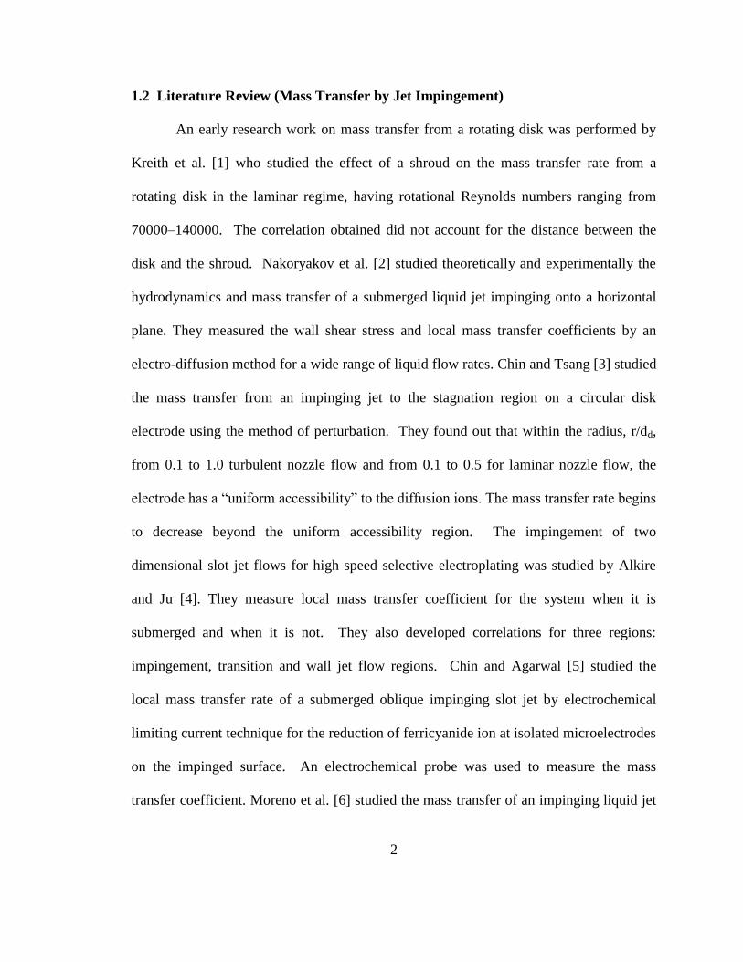
1.2 Literature Review (Mass Transfer by Jet Impingement)

An early research work on mass transfer from a rotating disk was performed by

Kreith et al. [1] who studied the effect of a shroud on the mass transfer rate from a

rotating disk in the laminar regime, having rotational Reynolds numbers ranging from

70000–140000. The correlation obtained did not account for the distance between the

disk and the shroud. Nakoryakov et al. [2] studied theoretically and experimentally the

hydrodynamics and mass transfer of a submerged liquid jet impinging onto a horizontal

plane. They measured the wall shear stress and local mass transfer coefficients by an

electro-diffusion method for a wide range of liquid flow rates. Chin and Tsang [3] studied

the mass transfer from an impinging jet to the stagnation region on a circular disk

electrode using the method of perturbation. They found out that within the radius, r/dd,

from 0.1 to 1.0 turbulent nozzle flow and from 0.1 to 0.5 for laminar nozzle flow, the

electrode has a “uniform accessibility” to the diffusion ions. The mass transfer rate begins

to decrease beyond the uniform accessibility region. The impingement of two

dimensional slot jet flows for high speed selective electroplating was studied by Alkire

and Ju [4]. They measure local mass transfer coefficient for the system when it is

submerged and when it is not. They also developed correlations for three regions:

impingement, transition and wall jet flow regions. Chin and Agarwal [5] studied the

local mass transfer rate of a submerged oblique impinging slot jet by electrochemical

limiting current technique for the reduction of ferricyanide ion at isolated microelectrodes

on the impinged surface. An electrochemical probe was used to measure the mass

transfer coefficient. Moreno et al. [6] studied the mass transfer of an impinging liquid jet

3

confined between two parallel plates theoretically and by experiments. The mass transfer

rate was characterized by an etching method in a cupric chloride etching solution and jet

instability on the etching rate within the central impingement zone was discussed. Chen

et al. [7] investigated experimentally the mass transfer between an impinging jet and a

rotating disk. The naphthalene sublimation technique was used in the experiment. The

experimental results showed that heat/mass transfer are divided into three regions which

are the impingement dominated region, the mixed region and the rotation dominated

region. It was concluded that the Sherwood number of a rotating disk with jet

impingement was the sum of two components governed by the impinging jet and the

rotating disk. Pekdemir and Davies [8] studied the mass transfer behavior of an

isothermal system when a rotating circular cylinder is exposed to a two dimensional slot

jet of air with a laminar flow. In the impingement dominated regime, they observed that

the rotation of disk did not influence heat transfer characteristics of the system, while the

jet impingement had a strong effect on the local heat transfer of the rotating disk. Chen

and Modi [9] investigated the mass transfer characteristics of a turbulent slot jet

impinging normally on a target wall with a confinement plate placed parallel to the target

plate examined using numerical simulations. The flow was modeled using a k-w

turbulence model. The Reynolds number simulated ranged from 450 to 20000, Prandtl or

Schmidt numbers from 0 to 2400 and the slot jets varied between 2 and 8 times the width

of the slot jet. Chen et al. [10] conducted experiment on mass and heat transfer for high

Schmidt numbers with a laminar jet impingement flow onto rotating and stationary disks.

The experiment used naphthalene sublimation technique where three regimes where

4

observed, namely the impingement dominated regime, the mixed regime and the rotation

dominated regime. Using a conical shaped impingement plate, Miranda and Campos [11]

investigated mass transfer in a laminar by impinging jet. The distance between the nozzle

and the plate was less than one nozzle diameter, the laminar flow was less than 1600, and

the Schmidt was up to 50000. Oduoza [12] worked on mass transfer on a heated

electrode by simulating high speed wire plating with simultaneous heat transfer in the

laminar region. The working fluid used for the study was ferricyanide. In the simulation,

it showed a distinct effect of thermally driven natural convection at a lower Reynolds

number and but as the Reynolds number increased, it merged with the Leveque solution.

Arzutuğ et al. [13] compared the mass transfer distribution from a jet to a plate between a

submerged conventional impinging jet (CIJ) and multichannel conventional impinging jet

(MCIJ). Electrochemical limiting diffusion current technique (ELDCT) was used to

measure the local mass transfer coefficients. The values that were obtained for the mean

mass transfer coefficients over the surface for CIJ and MCIJ were found to be relatively

close to each other with MCIJ having slightly higher values. Quiroz et al. [14] also used

the electrochemical limiting diffusion current technique (ELDCT) to measure the mass

transfer between parallel disk cells with the help of the Levique relation. Sedahmed et al.

[15] studied the rate of mass transfer between two immiscible liquids, an aqueous layer

and a mercury pool upon which an axial jet was impinging under turbulent flow

conditions and measured by electrochemical limiting diffusion limiting current technique

(ELDCT).

5

Sara et al. [16] measured the mass transfer coefficient using the ELDCT method

of an electrochemical system from an impinging liquid jet to a rotating disk in a fully

confined environment. The study used a rotational Reynolds number of up to 120000,

and a jet Reynolds number of up to 53000 with a non-dimensional jet-to-disk spacing of

2-8. They found out that the jet impingement had a considerable effect on the

enhancement of the mass transfer compared to the case of the rotating disk without jet.

The effects on mass/heat transfer on rotation by impingement jet were also studied by

Hong et al. [17]. Their research covered a wide range of rotational Reynolds numbers

(400 to 10,000) including laminar, turbulent and transitional regimes. Hong et al. [18]

investigated the mass transfer characteristics on a concave surface for rotating impinging

jets. A jet with Reynolds number of 5,000 was applied to the concave surface and a flat

surface. They found out that compared to flat surface, the heat/mass transfer on the

concave surface is enhanced with increasing the span-wise direction due to the curvature

effect, providing a higher averaged Sherwood value.

Research has also been done involving heat transfer in jet impingement processes.

Lallave et al [19] studied the characterization of conjugate heat transfer for a confined

liquid jet impinging on a rotating and uniformly heated solid disk of finite thickness and

radius. The study showed that the plate materials with higher thermal conductivity had a

more uniform temperature distribution at the solid–fluid interface, and the local heat

transfer coefficient increased with an increasing in Reynolds number which reduced the

wall to fluid temperature difference over the entire interface. Lallave and Rahman [20]

6

worked on conjugate heat transfer characterization of a partially–confined liquid jet

impinging on a rotating and uniformly heated solid disk of finite thickness and radius.

Even though a number of publications have considered the heat/mass transfer rate

effect of numerous parameters, not enough research has been done on mass transfer

during laminar jet impingement on a rotating disk in a fully confined environment using

an electrolyte. The intent of this research is to investigate the mass transfer effect in a

uniform laminar flow from the jet nozzle onto a rotating disk in a fully confined space.

The study parameter includes five jets Reynolds numbers, five rotational Reynolds

numbers and stationary disk, five heights measured from the nozzle to the target disk,

five Schmidt numbers, and different confinement plate shapes such as conical, convex,

and concave.

Present results offer a better understanding of the fluid mechanics and mass

transfer behavior of liquid jet impingement under confinement on top of a spinning target

because of the incorporation of the varying parameters. Even though no new numerical

technique has been developed, results obtained in this investigation are entirely new. The

numerical results showing the quantitative effects of different parameters as well as the

correlation for average Sherwood numbers will be practical guides for enhancement of

mass transfer during the electrolyte synthesis and etching processes.

7

1.3 Introduction (Heat Transfer in a Microchannel)

Microchannels of trapezoidal cross section are widely used in silicon-based

microsystems. The study of fluid flow and heat transfer is critical to the development of

these microsystems. This thesis presents a systematic analysis of fluid flow and heat

transfer processes during the magnetic heating of a magnetocaloric material which is

bonded to the substrate. The substrate has an array of trapezoidal channels through which

heat is transferred to the working fluid. When a magnetic field is imposed on a

magnetocaloric material, heat is generated. This results in increase in temperature of the

material. Similarly, the temperature drops during demagnetization when the field is

removed. The purpose of this thesis is to study the effects of change in different

geometrical and thermal parameters on fluid flow and heat transfer when a magnetic field

is applied to the substrate material.

8

1.4 Literature Review (Heat Transfer in a Microchannel)

Wu and Little [31] measured the friction factors of laminar gas flow in the

trapezoidal silicon/glass microchannels, and found that the surface roughness affected the

values of the friction factors even in the laminar flow, which is different from the

conventional macrochannel flow. Harley et al. [32] presented experimental and

theoretical results of low Reynolds number, high subsonic Mach number, compressible

gas flow in channels. Nitrogen, helium, and argon gases were used. Detailed data on

velocity, density and temperature distributions were obtained. The effect of the Mach

number on profiles of axial and transversal velocities and temperature were revealed.

Chen and Wu [33] investigated the microchannel flow in miniature TCDs (thermal

conductivity detectors). Effects of channel size and boundary conditions were examined

in details. It was found that the change in heat transfer rate in the entrance region depends

primarily on the thermal conductivity change in the conduction-dominant region. Qu et

al. [34] investigated heat transfer characteristics of water flowing through trapezoidal

silicon microchannels. A numerical analysis was carried out by solving a conjugate heat

transfer problem.

Rahman [35] presented new experimental measurements for pressure drop and

heat transfer coefficient in microchannel heat sinks. Tests were performed with devices

fabricated using standard Silicon <100> wafers. Channels of different depths (or aspect

ratios) were studied. Tests were carried out using water as the working fluid. The fluid

flow rate as well as the pressure and temperature of the fluid at the inlet and outlet of the

device, and temperature at several locations in the wafer were measured. These

9

measurements were used to calculate local and average Nusselt number and coefficient of

friction in the device. Toh et al. [36] studied the fluid flow and heat transfer in a

microchannel by number computation. The results of the numerical computations where

compared to experimental data for validation. Their research revealed that heat input

lowers frictional losses at mostly lower Reynolds numbers since an increase in

temperature leads to a decrease in viscosity thereby leading to smaller frictional losses.

Qu and Mudawar [37] also investigated the heat transfer behavior in a rectangular

microchannel. They observed that when the thermal conductivity of a substrate is

increased in which the fluid flows through while keeping all parameters constant, the

temperature at the base surface of the heat sink reduces. They concluded that a higher

laminar Reynolds number at 1400 will not be a fully developed flow in a microchannel

and as a result will lead to enhanced heat transfer. Wu and Cheng [38] observed the same

behavior of an approximate linear correlation between the Nusselt number and Reynolds

number at Re < 100. They studied what effect the surface roughness of the microchannel

and surfaces’ affinity for water (hydrophilic property) has on the Nusselt number. The

investigation showed that there is an increase in the laminar Nusselt number when the

surface roughness or hydrophilic property is increased. The apparent friction constant

also increased with an increase in the surface roughness.

Wu and Cheng [39] measured the friction factor of laminar flow of deionized

water in smooth silicon micro-channels of trapezoidal cross-section. The experimental

data were found to be in agreement within ±11% with an existing analytical solution for

an incompressible, fully developed, laminar flow under the no-slip boundary condition. It

10

was confirmed that Navier–Stokes equations are still valid for the laminar flow of

deionized water in smooth micro-channels having hydraulic diameter as small as 25.9

μm. For smooth channels with larger hydraulic diameters of 103.4–291.0 μm, transition

from laminar to turbulent flow occurred at Re = 1500–2000. Li et al. [40] conducted a

numerical simulation on a silicon-based microchannel heat sink. The finite difference

numerical code developed to solve the governing equations was the Tri-Diagonal Matrix

Algorithm. The behavior flow and the heat transfer were investigated to observe how the

geometric parameters of the channel and thermo-physical properties affect them. The

outcome of this study revealed that the thermo-physical properties of the liquid used in

the analysis can considerably affect both flow and heat transfer in the microchannel heat

sink. Mo et al. [41] studied the flow of nitrogen gas in a rectangular channel by forced

convection. The different parameter varied during the study showed considerable effect

on the heat transfer characteristic in the channel. The main parameters were temperature,

hydraulic diameter, and aspect ratio. The research revealed that heat addition had the

most influence on the system, followed by the channel aspect ratio, Reynolds number

which is a function of the hydraulic diameter, and Prandtl number.

Owhaib and Palm [42] experimentally investigated the heat transfer

characteristics of single-phase forced convection flow through circular microchannels.

The results were compared to correlations for heat transfer in macroscale channels. The

results showed good agreement between classical correlations and experimentally

measured data. Wu and Cheng [43] carried out a series of experiments to study different

boiling instability modes of water flowing in microchannels at various heat flux and mass

11

flux with the outlet of the channels at atmospheric pressure. Eight parallel silicon

microchannels with an identical trapezoidal cross-section were used in this experiment.

Morini et al. [44] investigated the rarefaction effects on the pressure drop for an

incompressible flow through silicon microchannels having a rectangular and trapezoidal

cross section. The roles of Knudsen number and the cross-section aspect ratio on the

friction factor reduction due to the rarefaction were pointed out. Chen and Cheng [45]

performed a visualization study on condensation of steam in microchannels etched in a

silicon <100> wafer that was bonded by a thin Pyrex glass plate from the top. Saturated

steam flowed through these parallel microchannels, whose walls were cooled by natural

convection of air at room temperature. Stable droplet condensation was observed near the

inlet of the microchannel. It was predicted that the droplet condensation heat flux

increases as the diameter of the microchannel is decreased. The experimental

investigation of heat transfer in a rectangular microchannel was also performed by Lee et

al. [46]. They explored the validity of classical correlations based on conventionalized

channels for predicting the thermal behavior in a single-flow. This study also showed

that at a given flow rate within the laminar region, the heat transfer coefficient will

increase with a decreasing channel size. In applying a uniform heat flux to a trapezoidal

microchannel, Cao et al. [47] showed the effect of velocity slip on the Nusselt number

and friction coefficient of the system. It was discovered that values of Nusselt number

for a slip flow was larger than that of a no-slip flow and an increase in aspect ratio will

result in an increase in fully Nusselt number. Hetsroni et al. [48] compared experimental

result based on theoretical and numerical results for heat transfer in a microchannel at

12

small Knudsen numbers. The effect of the geometric and axial heat flux parameters on

the system was analyzed. The thermal conduction through the working fluid, channel

walls and energy dissipation was observed with regards to the parameters.

Zhuo et al. [49] also studied the heat transfer behavior in both triangular and

trapezoidal microchannel by numerical and experimental processes. The intersection

angle between the temperature and velocity gradient was observed and the synergy for

Reynolds numbers below 100 was much better. The field synergy principle was

confirmed with an almost linear relationship between the Reynolds number and their

corresponding Nusselt number for Re < 100. Li et al. [50] showed through studies that

Nusselt number and heat transfer coefficient will reduce along the flow of a microchannel

with the least values at the outlet. Husain and Kim [51] used numerical methods in order

to optimized microchannel heat sink using a surrogate analysis and evolutionary

algorithm. In the optimization, the objective functions of thermal resistance and pumping

power in the microchannel where formulated to evaluate the performance of the heat

sink. Rahman et al. [52] investigated the convective heat transfer related to a magnetic

field in a circular microchannel with rectangular substrate. The heat source was from

gadolinium, a magnetocaloric material that generates heat within a magnetic field and

different parameters where varied to see the influence on the heat transfer coefficient. Li

and Kleinstreuer [53] compared the thermal conductivity model for nanofluids; one

involved the application of a model based on the Brownian motion induced micro-mixing

and the other was based on Navier-Stokes. The study was done on the flow of nanofluids

pure water and CuO-water through a trapezoidal microchannel. Their research revealed

13

that nanofluids improved thermal performance of microchannel mixture flow but with a

pressure drop.

Hooman [54] presented investigation on the convective characteristics of a

rectangular microchannel with a porous medium while factoring parameters such as

temperature jump, velocity profile, duct geometry, friction factor and slip coefficient.

Their influence on the Nusselt number was analyzed. Hasan et al. [55] studied the effect

of channel geometry on a microchannel heat exchanger. Numerical simulations were

carried out to solve developing flow and conjugate heat transfer. The shapes investigated

include square, rectangular, trapezoidal and iso-triangle. Their investigation showed that

with the parameters used, when the volume of a channel is decreased or the number of

channels are increase, heat transfer increases, pressure drops and pumping power

increases. This study within the parameters used showed the circular channel having the

most effective thermal efficiency. Hsieh and Lin [56] performed experiment to

determine the thermal characteristics of a fluid in rectangular microchannel. The fluids

used in the experiments were deionized water, methanol and ethanol solutions. The

parameters were aspect ratio, hydraulic diameter, Reynolds numbers, surface conditions,

thermal properties and the different fluids. From within the extent of these parameters, it

was observed that the hydrophilic surfaces had higher local heat transfer coefficients than

that of hydrophobic for all test fluids. Chen et al. [57] studied the thermal behavior of

heat transfer in different shapes of microchannels. These shapes include trapezoidal,

rectangular and triangular shapes. In the study, the Nusselt number was seen to be

highest at the inlet of the heat sink and least at the outlet. In comparison with the

14

different shapes of microchannel that were studied, it was observed that the triangular

shaped model had the most thermal efficiency.

DeGregoria et al. [58] tested an experimental magnetocaloric refrigerator

designed to operate within a temperature range of about 4 to 80 K. Helium gas was used

as the heat transfer fluid. A single magnet was used to charge and discharge two in-line

beds of magnetocaloric material. Zimm et al. [59] investigated magnetic refrigeration for

near room temperature cooling. Water was used as the heat transfer fluid. A porous bed

of magnetocaloric material was used in the experiment. It was found that using a 5T

magnetic field, a refrigerator reliably produces cooling powers exceeding 500W at

coefficient of performance 6 or more. Pecharsky and Gschneidner [60] discussed new

magnetocaloric materials with respect to their magnetocaloric properties. Recent progress

in magnetocaloric refrigerator design was reviewed.

The objective of the present investigation is to take a step ahead in study of

micro-channels of trapezoidal cross section by investigating composite trapezoidal

channels. A composite trapezoidal microchannel structure is formed by bonding a slab of

gadolinium with silicon wafer where microchannels of trapezoidal cross section have

been etched out of the silicon substrate. The study presents different parametric variations

and its effect on the fluid flow and heat transfer characteristics of the channel.

15

CHAPTER 2

ANALYSIS OF MASS TRANSFER BY JET IMPINGEMENT

2.1 Mathematical Model

The diagram of figure 2.1 is a schematic of the problem being analyzed. It

involves an axi-symmetric feature with the ejection of liquid jet from the nozzle which

impinges on a rotating disk. Figure 2.1a and 2.1b are the 2D and 3D schematics

respectively. The nozzle diameter, dn is 0.15cm which is kept as a constant function of

Rej used in simulation and calculations of local and average Sherwood number in

equations (13 and 14). The rotating disk has a diameter, dd of 1.5cm where a 10 to 1 ratio

with dn was intended. Dimensionless height, is calculated H/dn. In analysis, is made

to vary to observe the effect it has on the mass transfer rate. The numerical model

parameters include a Newtonian fluid with constant properties, an incompressible flow

under laminar and steady state conditions. As part of this computational analysis, the

system under study was under isothermal conditions neglecting the heat transfer effects

of the energy equation. The equations describing the conservation of mass, momentum

(r,, and z directions respectively) can be written as [28].

0z

V

r

V

r

V Zrr

(1)

2

r

2

r

2

r

2

r

2

f

rZ

2

θrr

r

V

z

V

r

V

r

1

r

Vν

r

p

ρ

1

z

VV

r

V

r

VV (2)

16

2

θ

2

θ

2

θ

2

θ

2

θ

Z

θrθ

rr

V

z

V

r

V

r

1

r

Vν

z

VV

r

VV

r

VV (3)

2

Z

2

Z

2

Z

2

f

ZZ

Zr

z

V

r

V

r

1

r

Vν

z

p

ρ

1g

z

VV

r

VV (4)

The mass transport equation of momentum accommodates the chemical species in

the following form:

2

i

2

22

i

2

iiz

iθ

ir

z

C

θr

C

r

Cr

rrD

z

CV

θr

CV

r

CV (5)

In addition, the ion mass flux (moles/area-time) which involves the transfer of

ions between an electrolyte and the electrode is defined by:

)cK(cN int (6)

Where N is ion mass flux, which is related to the mass transfer coefficient, K, c∞ is the

concentration of ions in the bulk fluid and cint is the concentration of ions on the

interface. The following boundary conditions were used.

0r

fC

0,r

zV

0,r

Vθ

V:Hz00,rAt

(7)

atmd pp:δz0,rrAt (8)

rΩθ

V0,z

Vr

V:d

rr00,zAt (9)

jT

fT0,

θV

rV,

jV

zV:

2

dr0H,zAt (10)

0z

C0,

zV

rV

θV:

prr

2

dH,zAt f

(11)

The boundary conditions applied to the flow is a no–slip condition where the

velocity parallel to the walls and on the wall is zero. The formula used to determine the

17

average mass transfer coefficient has the same form that the average heat transfer

coefficient equation used by Rahman and Lallave [20].

drd

r

0j

Cint

CrK

jC

intC2

dr

2

avK

(12)

Where Cint is the average concentration at the solid–liquid interface, Cj and Cint are the jet

and interface concentrations, respectively. The local and average Sherwood numbers are

calculated according to the following expressions:

D

dKSh n

(13)

D

dKSh nav

av

(14)

18

Figure 2.1a Confined liquid jet impingement between a rotating disk and an

impingement plate, two-dimensional schematic.

Figure 2.1b Confined liquid jet impingement between a rotating disk and an

impingement plate, three-dimensional schematic.

19

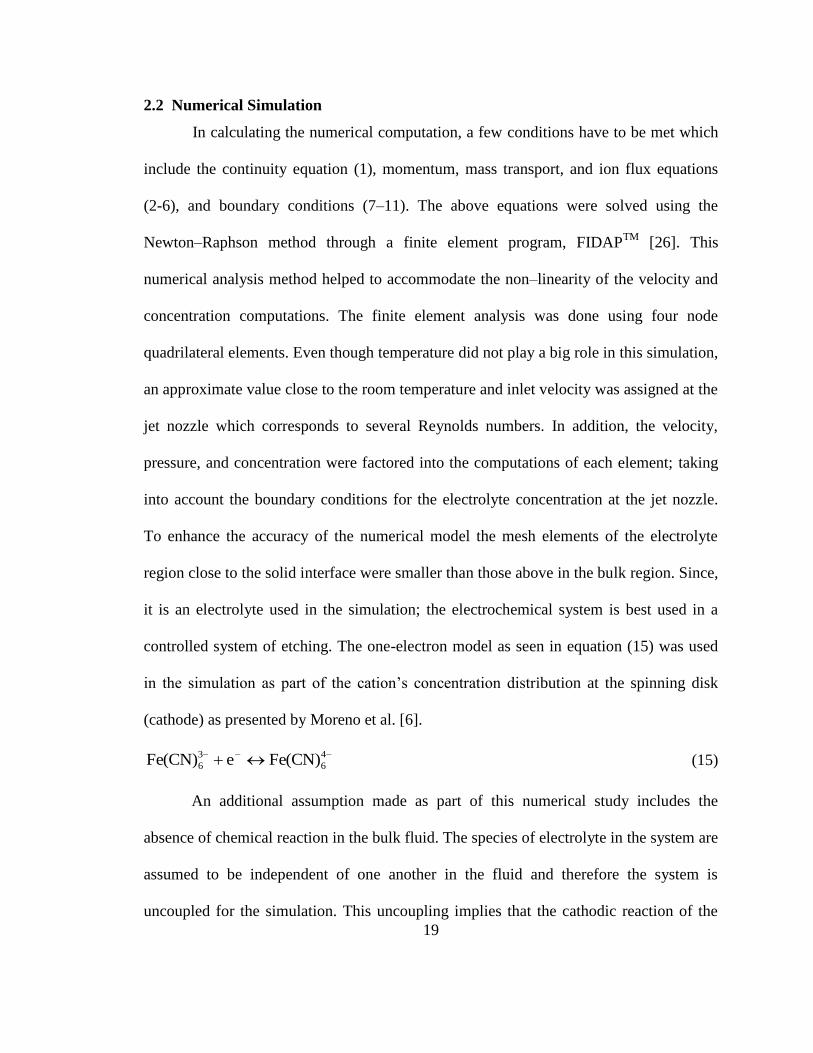
2.2 Numerical Simulation

In calculating the numerical computation, a few conditions have to be met which

include the continuity equation (1), momentum, mass transport, and ion flux equations

(2-6), and boundary conditions (7–11). The above equations were solved using the

Newton–Raphson method through a finite element program, FIDAPTM

[26]. This

numerical analysis method helped to accommodate the non–linearity of the velocity and

concentration computations. The finite element analysis was done using four node

quadrilateral elements. Even though temperature did not play a big role in this simulation,

an approximate value close to the room temperature and inlet velocity was assigned at the

jet nozzle which corresponds to several Reynolds numbers. In addition, the velocity,

pressure, and concentration were factored into the computations of each element; taking

into account the boundary conditions for the electrolyte concentration at the jet nozzle.

To enhance the accuracy of the numerical model the mesh elements of the electrolyte

region close to the solid interface were smaller than those above in the bulk region. Since,

it is an electrolyte used in the simulation; the electrochemical system is best used in a

controlled system of etching. The one-electron model as seen in equation (15) was used

in the simulation as part of the cation’s concentration distribution at the spinning disk

(cathode) as presented by Moreno et al. [6].

4

6

3

6 Fe(CN)eFe(CN) (15)

An additional assumption made as part of this numerical study includes the

absence of chemical reaction in the bulk fluid. The species of electrolyte in the system are

assumed to be independent of one another in the fluid and therefore the system is

uncoupled for the simulation. This uncoupling implies that the cathodic reaction of the

20

rotating disk is independent of the flow or diffusion of the fluid and because of this

assumption, the etch rate or chemical reaction can be ignored in the analysis. The

properties of the following electrolytes (NaOH), K3[Fe(CN)6], and HCl, were obtained

from Moreno et al.[6], Sara et al. [16], Quiroz et al.[14], Guggenheim [21] and Fary

[22]. For this simulation, the Soret effect is negligible therefore, the flow was assumed

to have only a mass transfer by convection and a mass transfer by diffusion which is as a

result of a concentration gradient which can best be described by Fick’s law.

ii CDG (16)

During the iteration, the values begin to converge relative to their previous values

and the residuals are summed up for each variable which is less that 10-6

. To verify that

the conservation of mass was met, the flow rate at the outlet was compared with the

flowrate at the nozzle of the jet to make sure their sum is zero. The suitable number of

element to be used in the simulation was determined by an independent systematic pick.

A graph of the best of meshes can be seen in figure 2.3. The most accurate mesh of model

shows a grid size of 20 x 500 divisions of elements in the axial (z) and radial (r)

directions, respectively. Numerical results for this grid compared to the others gave

almost identical results with an average margin error of 1.2%. The result of the

electrolyte interface concentration distribution obtained from the finite element analysis

is used to calculate the mass transfer coefficient, local and average Sherwood numbers.

21

2.3 Results and Discussion

The mesh used for simulation can be seen in figure 2.2 and figure 2.3 which

shows the best of all meshes plotted together. Figure 2.3 facilitates the process of

choosing an optimum mesh with the lowest number of percentage difference. The mesh

used is the 20x500 mesh grid spacing having the smallest number of divergence when

compared to the others at an average of 1.21%. The amount of grid spacing in the vertical

direction was made denser under the jet nozzle to accommodate the mass transport

equation. The Schmidt number focused on in this study results in a thin boundary layer

and for this reason, the closer the grid spacing was to the interface the smaller grids got in

the horizontal direction to facilitate the transport equation of the ions.

Figure 2.2 Mesh plot for a grid spacing of 20 x 500 in the axial and radial directions.

22

Figure 2.3 Dimensionless interface temperature distributions for different number of

elements in r and z directions (Rej=1000, Rer=2310, =1.0, and Sc=2315).

0.00

0.05

0.10

0.15

0.20

0.25

0.30

0.35

0.40

0 0.1 0.2 0.3 0.4 0.5 0.6 0.7 0.8 0.9 1

Inte

rfa

ce C

on

cen

trati

on

, C

int (g

/cm

3)

Dimensionless Radial Distance, r/R

NZ x NR = 10 x 280

NZ x NR = 20 x 500

NZ x NR = 30 x 290

NZ x NR = 35 x 320

NZ x NR = 40 x 340

.

23

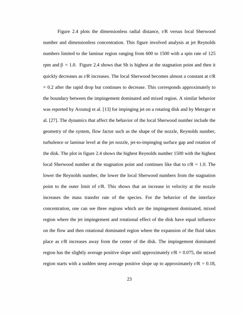
Figure 2.4 plots the dimensionless radial distance, r/R versus local Sherwood

number and dimensionless concentration. This figure involved analysis at jet Reynolds

numbers limited to the laminar region ranging from 600 to 1500 with a spin rate of 125

rpm and = 1.0. Figure 2.4 shows that Sh is highest at the stagnation point and then it

quickly decreases as r/R increases. The local Sherwood becomes almost a constant at r/R

= 0.2 after the rapid drop but continues to decrease. This corresponds approximately to

the boundary between the impingement dominated and mixed region. A similar behavior

was reported by Arzutuğ et al. [13] for impinging jet on a rotating disk and by Metzger et

al. [27]. The dynamics that affect the behavior of the local Sherwood number include the

geometry of the system, flow factor such as the shape of the nozzle, Reynolds number,

turbulence or laminar level at the jet nozzle, jet-to-impinging surface gap and rotation of

the disk. The plot in figure 2.4 shows the highest Reynolds number 1500 with the highest

local Sherwood number at the stagnation point and continues like that to r/R = 1.0. The

lower the Reynolds number, the lower the local Sherwood numbers from the stagnation

point to the outer limit of r/R. This shows that an increase in velocity at the nozzle

increases the mass transfer rate of the species. For the behavior of the interface

concentration, one can see three regions which are the impingement dominated, mixed

region where the jet impingement and rotational effect of the disk have equal influence

on the flow and then rotational dominated region where the expansion of the fluid takes

place as r/R increases away from the center of the disk. The impingement dominated

region has the slightly average positive slope until approximately r/R = 0.075, the mixed

region starts with a sudden steep average positive slope up to approximately r/R = 0.18,

24

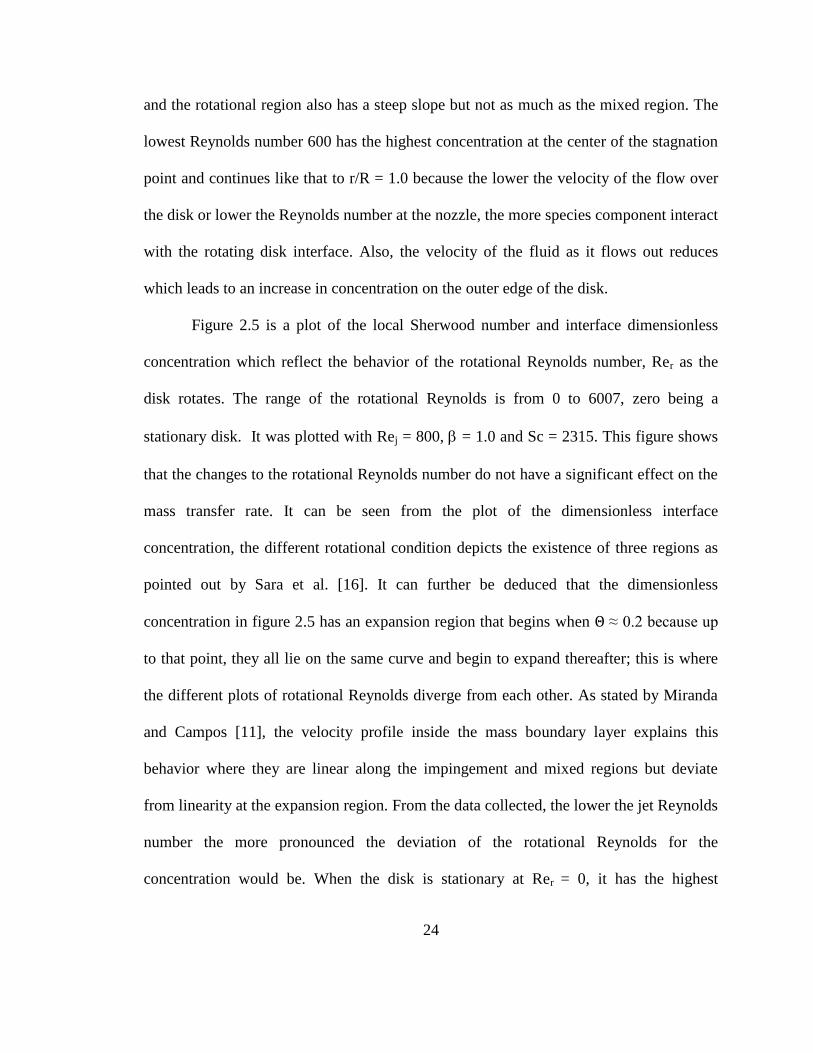
and the rotational region also has a steep slope but not as much as the mixed region. The

lowest Reynolds number 600 has the highest concentration at the center of the stagnation

point and continues like that to r/R = 1.0 because the lower the velocity of the flow over

the disk or lower the Reynolds number at the nozzle, the more species component interact

with the rotating disk interface. Also, the velocity of the fluid as it flows out reduces

which leads to an increase in concentration on the outer edge of the disk.

Figure 2.5 is a plot of the local Sherwood number and interface dimensionless

concentration which reflect the behavior of the rotational Reynolds number, Rer as the

disk rotates. The range of the rotational Reynolds is from 0 to 6007, zero being a

stationary disk. It was plotted with Rej = 800, = 1.0 and Sc = 2315. This figure shows

that the changes to the rotational Reynolds number do not have a significant effect on the

mass transfer rate. It can be seen from the plot of the dimensionless interface

concentration, the different rotational condition depicts the existence of three regions as

pointed out by Sara et al. [16]. It can further be deduced that the dimensionless

concentration in figure 2.5 has an expansion region that begins when Θ ≈ 0.2 because up

to that point, they all lie on the same curve and begin to expand thereafter; this is where

the different plots of rotational Reynolds diverge from each other. As stated by Miranda

and Campos [11], the velocity profile inside the mass boundary layer explains this

behavior where they are linear along the impingement and mixed regions but deviate

from linearity at the expansion region. From the data collected, the lower the jet Reynolds

number the more pronounced the deviation of the rotational Reynolds for the

concentration would be. When the disk is stationary at Rer = 0, it has the highest

25

concentration at the outer radius of the disk compared to when the disk is rotating. The

velocity can once again be used to explain this action. An increase in velocity as a result

of the rotational speed leads to less concentration of the species on the disk. Therefore,

the increment of spinning rate or rotational Reynolds number (Rer) will decrease the

dimensionless concentration, (Θ) as seen in figure 2.5.

The distance between the nozzle and the rotating disk is simulated at different

heights. Figure 2.6 shows the result of this action on the local Sherwood number and

dimensionless concentration over the dimensionless radial distance for = 0.5 to 20. The

conditions applied to the simulation include Rej = 1500 and Rer = 2310. From the data,

the highest dimensionless height = 2.0 has the higher mass transfer rate than when =

0.5 at the center of the disk, but towards the end of the disk, = 0.5 has a higher mass

transfer rate than when it is 2.0. This occurs because of the difference in the length of

their potential core and the characteristics of the jet. The graph shows that an increment

of the dimensionless height () will cause the species concentration on the disk to

increase along the dimensionless radial distance (r/R). The rotation dominated region on

the concentration data begins at a point that corresponds with proportionality to the

dimensionless height () at the dimensionless radial distance of r/R 0.2. The local

Sherwood number shows the same behavior at figure 2.4 and 2.5 but as the dimensionless

height increases, the local Sherwood number increases for each radius in the expansion

region. The axis of the disk has the highest local Sherwood value which decreases rapidly

with a very steep slope and when c/C ≈ 2.2, there is a rapid change to a gentle slope

which is as a result of the increase in thickness of the mass boundary layer in the mixed

26

region. As the flow begins to expand, a minimum value of local Sherwood number is

reached.

Figure 2.4 Local Sherwood number and dimensionless concentration for different jet

Reynolds numbers (=1.0, Rer=2310, nickel disk, and Sc=2315).

0

50

100

150

200

250

300

350

400

0

500

1000

1500

2000

2500

3000

3500

0.0 0.1 0.2 0.3 0.4 0.5 0.6 0.7 0.8 0.9 1.0

Dim

ensi

on

less

Co

nce

ntr

ati

on

, Q

(C

int/

Cj)

Lo

cal

Sh

erw

oo

d N

um

ber

, S

h

Dimensionless Radial Distance (r/R)

Sh, Re = 650

Sh, Re = 800

Sh, Re = 1000

Sh, Re = 1250

Sh, Re = 1500

Q, Re = 750

Q, Re = 800

Q, Re = 1000

Q, Re = 1250

Q, Re = 1500

Sh, Rej= 650

Sh, Rej=800j

Sh, Rej=1000j

Sh, Rej=1250j

Sh, Rej=1500

Q, Rej=650

Q, Rej=800j

Q, Rej=1000j

Q, Rej=1250j

Q, Rej=1500

27

Figure 2.5 Local Sherwood number and dimensionless concentration for different

rotational Reynolds numbers (=1.0, nickel disk, Rej=800, and Sc=2315).

0

50

100

150

200

250

300

0

130

260

390

520

650

780

910

1040

1170

1300

0.0 0.1 0.2 0.3 0.4 0.5 0.6 0.7 0.8 0.9 1.0D

imen

sio

nle

ss C

on

cen

tra

tio

n,

Q (

Cin

t/C

j)

Lo

cal

Sh

erw

oo

d N

um

ber

, S

h

Dimensionless Radial Distance, (r/R)

0

2310

4158

5082

6006

c0

c2310

c4158

c5082

c6006

Q, Rer= 0

Q, Rer = 2310j

Q, Rer = 4159j

Q, Rer = 5083

Q, Rer = 6007

Sh, Rer= 0Sh, Rer = 2310Sh, Rer = 4159Sh, Rer = 5083Sh, Rer = 6007

28

Figure 2.6 Local Sherwood number and dimensionless concentration for different

dimensionless heights (Rej=1500, Rer=2310, and Sc=2315).

0

50

100

150

200

250

300

350

0

500

1000

1500

2000

2500

3000

3500

4000

0.0 0.1 0.2 0.3 0.4 0.5 0.6 0.7 0.8 0.9 1.0

Dim

ensi

on

less

Co

nce

ntr

ati

on

, Q

(C

int/

Cj)

Lo

cal

Sh

erw

oo

d N

um

ber

, S

h

Dimensionless Radial Distance (r/R)

Sh, ß = 0.5

Sh, ß = 0.75

Sh, ß = 1.0

Sh, ß = 1.5

Sh, ß = 2.0

H/d =0.5c

H/d =0.75c

H/d =1.0c

H/d =1.5c

H/d =2.0c

Sh, = 0.5Sh, = 0.75Sh, = 1.0Sh, = 1.5Sh, = 2.0

Q, = 0.5

Q, = 0.75Q, = 1.0Q, = 1.5Q, = 2.0

`

29

Figure 2.7 Average Sherwood numbers with jet Reynolds numbers at various

rotational Reynolds numbers (=1.0, nickel disk, and ferricyanide electrolyte and

Sc=2315).

30

32

34

36

38

40

42

44

46

48

50

0 2000 4000 6000

Av

era

ge

Sh

erw

oo

d N

um

ber

, S

ha

vg

Rotational Reynolds, Rer

650

J800

J1000

J1250

1500

Rej = 650

Rej = 800

Rej = 1000

Rej = 1250

Rej = 1500

30

In figure 2.7, the average Sherwood number was plotted for different values of jet

Reynolds at = 1.0 against rotational Reynolds’ values. The average Sherwood number

increases with a relatively small difference when the rotational speed is increased which

points out the fact that it has little effect on the outcome of the average Sherwood

number. The result of the average Sherwood number shows that the effect of the mass

transfer influenced by the rotational Reynolds is relatively trivial compared to the

influence by the jet Reynolds. This shows that the impingement on the disk dominates the

flow of the fluid with the spin rates that were used for the simulations and that the critical

velocity of the rotational speed was not attained. Figure 2.7 also shows that the jet

Reynolds greatly affects the results of the Shavg. The results obtained in figure 2.7 are

similar to those of previous works. It is quite obvious that the three regions of flow

previously mentioned can no longer be observed because the curves are smoother since

average Sherwood number is now cumulative, and the rapid changes are attenuated by

the sum of the previous values.

Figure 2.8 shows the investigation of how affects Shavg for 1500Re600 j

where rad/s 13.09 . The length of the potential core has an effect on the local

Sherwood and as a result it has an influence on the average Sherwood number because as

increases, Shavg decreases. Another factor causing the decrease in Shavg is the increased

decay in average velocity as height of the nozzle from the rotating disk increases. As the

nozzle to target spacing increases, there are more instances where there is mixing of

induced turbulence occurs and the fluid does not expand as much as when the spacing is

smaller. With the increasing distance with the nozzle of the jet, a large portion of the

31

disk will stay inside the low velocity region of the jet. Therefore, the mass transfer rate

will decrease with an increasing distance from the nozzle of the jet.

Figure 2.9 shows the investigation of how 1.15β for Schmidt numbers

2472Sc1720 affects Shavg over 1500Re600 j at rad/s 13.09 . It depicts Shavg

increasing with Sc. The Schmidt number can be used to optimize the kinematic viscosity

or diffusion coefficient needed for a system. It can also be interpreted as the average

Sherwood number increasing with an increase in kinematic viscosity or decrease in

diffusion coefficient which is suitable in simulating fluids at specific properties. The

lower the Schmidt number the less the local Sherwood number over the radial direction

will be and therefore lead to a decline in the average mass transfer rate over the disk.

Figure 2.10 is a comparison between electrolytes. These electrolytes are

potassium ferricyanide (K3[Fe(CN)6] ) being replaced with Sodium Hydroxide (NaOH)

and the other is Hydrochloric acid (HCl). Their properties from Fary [22] and

Guggenheim [21] give us Sc = 791 and 655 at 25deg ⁰C for HCl and NaOH respectively

because of their much larger diffusion coefficient. The difference in Sc between

K3[Fe(CN)6 at 2315 and the other two electrolytes being compared to it is very different

from the ferricyanide having the highest concentration distribution followed by

Hydrochloric acid and then Sodium Hydroxide. The trend seen from this figure shows

that the lower the Schmidt number, the lower the distribution of concentration.

32

Figure 2.8 Average Sherwood number with jet Reynolds number at different

dimensionless nozzle to target spacing (Rer=2310, and Sc=2315).

20

25

30

35

40

45

50

55

60

65

70

0.50 0.75 1.00 1.25 1.50 1.75 2.00

Av

era

ge

Sh

erw

oo

d N

um

ber

, S

ha

vg

Dimensionless Nozzle to Target Spacing,

J650

J800

J1000

J1250

J1500

Re = 650

Re = 800

Re = 1000

Re = 1250

Re = 1500

33

Figure 2.9 Average Sherwood number with jet Reynolds number at different Schmidt

number (=1.15, nickel disk, ferricyanide electrolyte, and Rer=5082).

25

27

29

31

33

35

37

39

41

43

45

1700 1900 2100 2300 2500

Av

era

ge

Sh

erw

oo

d N

um

ber

, S

ha

vg

Schimdt Number, Sc

J650J800J1000J1250J1500

Rej = 650

Rej = 800

Rej = 1000

Rej = 1250

34

Figure 2.10 Dimensionless concentration for different electrolytes - NaOH, HCl,

3

6Fe(CN) (Rej=650, Rer=0, and =1.0).

0

50

100

150

200

250

300

0 0.2 0.4 0.6 0.8 1

Lo

cal

Sh

erw

oo

d N

um

ber

, S

h

Dimensionless Radial Distance (r/R)

Conc, Ferricyanide

Conc, Hydrochloric Acid

Conc, Sodium Hydroxide

Q, Ferricyanide

Q, Hydrochloric Acid

Q, Sodium Hydroxide

35

Figure 2.11 Local Sherwood number and dimensionless concentration over

dimensionless radial distance for different impingement plate geometries, nickel disk

with ferricyanide electrolyte (Rej=1000, Rer=5082, =1.15, and Sc=2315).

0

50

100

150

200

250

0

500

1000

1500

2000

2500

3000

0 0.2 0.4 0.6 0.8 1

Dim

ensi

on

less

Co

nce

nct

rati

on

, Q

(Cin

t/C

j)

Lo

cal

Sh

erw

oo

d N

um

ber

, S

h

Dimensionless Radial Distance, r/R

Sh, Parallel

Sh, Conical

Sh, Concave

Sh, Convex

Q, Parallel

Q, Conical

Q, Concave

Q, Convex

36

The graph in fig. 2.11 shows the distribution of mass transfer of local Sherwood

numbers and dimensionless concentration (Θ) over r/R for different confinements plates

at Rej = 1000 and Sc = 2315. The change in geometries is only with the confinement

plate which are conical, convex and concave shaped relative to the rotating disk. Figure

2.11 plot shows the three geometries being compared to the parallel confinement plate

used in this study. For the range of parameters used, the values of the Sh coincide for

most part of the disk except for the range 025.0R/r0 where the conical shaped

impingement plate starts with highest local Sherwood number and the parallel begins

with the lowest. The dimensionless radial distance of r/R = 0.025 is equivalent to a radius

0.035cm. When comparing a parallel confinement plate to a conical plate, Miranda and

Campos [11] study showed that lower Reynolds and Schmidt numbers create a clear

distinction of local Sherwood number results at the expansion region.

At the outer edge of the disk, the mass transfer rates are still almost the same with

the parallel disk still having the lowest Sherwood numbers and the convex confinement

plate having the highest. The conical shape had the highest Shavg followed by the concave

with the parallel impingement plate having the lowest. For the dimensionless

concentration part of the graph, the behavior is very much different. Starting with the

impingement region, they all start out alike and this can be explained by the fact that they

approximately have the same impingement plate shape within this region. At the region

that is dominated by rotation, the interface concentration begin to behave differently and

at this region the shape on the confinement plate begins to play a big role on the

concentration distribution on the disk. From the various confinement plate geometries

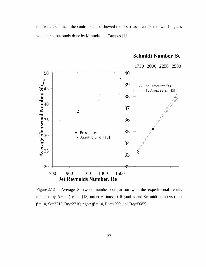
37

that were examined, the conical shaped showed the best mass transfer rate which agrees

with a previous study done by Miranda and Campos [11].

Figure 2.12 Average Sherwood number comparison with the experimental results

obtained by Arzutuğ et al. [13] under various jet Reynolds and Schmidt numbers (left:

=1.0, Sc=2315, Rer=2310; right: (=1.0, Rej=1000, and Rer=5082).

32

33

34

35

36

37

38

39

40

0 250 500 750 1000 1250 1500 1750 2000 2250 2500

20

25

30

35

40

45

50

700 900 1100 1300 1500 1700 1900 2100

Schmidt Number, Sc

Av

era

ge

Sh

erw

oo

d N

um

ber

, S

ha

vg

Jet Reynolds Number, Re

Present results

Arzutug et al. [8]

Sc Present results

Sc Arzutug et al. [8]

rrrbrbrbrbrg

rrrbrbrbr

Present results

- Arzutuğ et al. [13]

Sc Arzutuğ et al. [13] [13]

38

Figure 2.13 Average Sherwood number comparison with other studies within the core

region for various Schmidt numbers ( =1.0, Rej=800, Rer=2310).

0

40

80

120

160

200

240

280

320

360

1700 1900 2100 2300 2500

Av

era

ge

Sh

erw

oo

d N

um

ber

, S

ha

vg

Schmidt Numbers, Sc

Present Study

Chin & Tsang[1]

Sara[12]

Wang[27]

39

Figure 2.14 Comparison of predicted average Sherwood number using Equation 17

with present numerical data.

0

20

40

60

80

0 20 40 60 80

Act

ua

l A

ver

ag

e S

her

wo

od

Nu

mb

er,

Sh

av

g

Predicted Average Sherwood Number, Shavg

40

Figure 2.12 shows two different average Sherwood number comparison for a

range of jet Reynolds and Schmidt numbers. The right plot shows a varying jet Reynolds

number and the left shows a range of Schmidt number. This is an attempt to show how

close the present result obtained comes close to the correlation gotten by Arzutuğ et al.

[13]. The results of the plot on the left side were obtained for 1500Re800 j with Sc =

2315 at rad/s 13.09 . The average difference with the results from this plot was an

absolute 4.9% with a maximum of 10.3%. On the right graph, the comparison was done

at Rej = 1000 and Rer = 5082. The average difference here was 0.6% with the highest

deviation of 1% from Arzutuğ et al. [13].

The illustrations shown in fig. 2.13 are used to discuss the behavior of the average

Sherwood number within the impingement dominated zone. Figure 2.13 shows the

average Sherwood data in the impingement zone of present study, correlations obtained

by Chin and Tsang [3], Sara et al. [16], and Wang et al. [25] on a flat surface. The

Sherwood number is used to show the mass transfer in a dimensionless parameter versus

the Schmidt number of the electrolyte. The thicker line shows the finite element analysis

results of present study. The computations involved had a jet Reynolds number (Rej=800)

with a range of 24721720 Sc . In this impingement zone with the parameters used, the

Sherwood number were close to being proportional the square root of Rej while being

proportional to the cubic root of the Sc. The average Sherwood number in the core region

compared to Chin and Tsang [3], Sara et al. [16], and Wang et al. [25] shows an absolute

difference that range from 1 to 17% and had an average absolute difference of 7.73%.

41

A correlation for the average Sherwood number developed used the following

parameters Rej, Rer, , and Sc as variables. In this correlation, various parameters were

used and the data point employed corresponded with the electrolyte having a Sc =

2315(where =0.01275 cm2/s). The Prandtl number exponent of 0.4 from Martin’s

equation [23] for a single confined liquid jet impingement was kept constant as part of

present numerical correlation. The least square curve-fitting technique was adopted to

develop the correlation and the least square fit of the corresponding logarithmic equation.

The behavior of the average Sherwood number with the various parameters determined

the signs for the exponents. The correlation obtained for the present study can be seen in

equation (17) and illustrated in figure 2.14.

Shavg = 0.404.Rej

0.286Rer

0.0074

-0.714Sc

0.33 (17)

The highest absolute percentage difference between the actual Shavg and the

predicted results was 10.20% with an average absolute percentage difference of 3.89%.

The data of dimensionless parameters used for the correlation of this study take into

account jet Reynolds number 1500Re650 j , rotational Reynolds number, 6007Re0 r

, dimensionless height, 0.25.0 , Schmidt number, 2472Sc1720 , and geometrical

confinement plates: conical, convex, and concave layout. The present study correlation of

a liquid jet impingement on a rotating disk in a fully confined space can help in

predicting the mass transfer rates during the electrolyte synthesis as a process, especially

for etching processes.

42

CHAPTER 3

ANALYSIS OF HEAT TRANSFER IN A TRAPEZOIDAL

MICROCHANNEL

3.1 Modeling and Simulation

The physical configuration of the system used in the present investigation is

schematically shown in figure 3.1. A slab of gadolinium is placed on the top of the

channel and bonded with the silicon wafer in such a way that a part of heat generated in

gadolinium is directly dissipated to the working fluid whereas part is conducted through

the silicon structure. Neglecting the effects of inlet and outlet plenums, it was assumed

that the fluid enters the channel with a uniform velocity and temperature. The applicable

differential equations for the conservation of mass and momentum in the Cartesian

coordinate system are [61],

0z

w

y

v

x

u

(18)

])[(x

utvv

xx

p

ρ

1

z

uw

y

uv

x

uu

])[(])[(z

utvv

zy

utvv

y

(19)

])[(x

vtvv

xy

p

ρ

1

z

vw

y

vv

x

vu

])[(])[(z

vtvv

zy

vtvv

y

(20)

])[(x

wtvv

xz

p

ρ

1

z

ww

y

wv

x

wu

])[(])[(

z

wtvv

zy

wtvv

y

(21)

43

The k-ε model was used for the simulation of turbulence. In this model, equations

governing the conservation of turbulent kinetic energy and its rate of dissipation were

solved. These equations can be expressed as,

ε2

y

w2

x

w2

z

v2

x

v2

z

u2

y

u

tv

z

k

kζ

tvv

zy

k

kζ

tvv

yx

k

kζ

tvv

xz

kw

y

kv

x

ku

])()()()()()[(

])[(])[(])[(

(22)

k

2ε

2C

2

y

w2

x

w2

z

v2

x

v2

z

u2

y

u

tvk

ε

1C

z

ε

εζ

tvv

zy

ε

εζ

tvv

yx

ε

εζ

tvv

xz

εw

y

εv

x

εu

])()()()()()[(

])[(])[(])[(

(23)

/ε2

kμCtv (24)

The empirical constants appearing in equations (22)-(24) are given by the following

values, Cμ=0.09, C1=1.44, C2=1.92, σk=1.0, σε=1.3. These values hold good for high

Reynolds numbers. For low Reynolds number the values of constants are [62],

)3λ

0.008yλ

0.01yexp(1μC (24a)

Where, 2/1)//(

kyy (24b)

)10/exp(1.14.1

yk

(24c)

)10/exp(0.13.1 y (24d)

44

The energy equation in the fluid region is

])[(2

z

fT

2

2y

fT

2

2x

fT

2

tPr

tvα

z

fT

wy

fT

vx

fT

u

(25)

The equation for steady state heat conduction for gadolinium is [63],

0

gk

0g

2z

gT

2

2y

gT

2

2x

gT

2

(26a)

The equation for steady state heat conduction for silicon is [63],

02

z

sT

2

2y

sT

2

2x

sT

2

(26b)

To complete the physical model equations (18) – (26) are subjected to following

boundary conditions,

At z=0, at fluid inlet, u=0, v=0, w=win, T= Tin (27)

At z=0 on solid surfaces of silicon and gadolinium

0z

Ts

, 0

z

Tg

(28)

At z=L, at fluid outlet, p=0 (29)

At z=L, on solid surfaces of silicon and gadolinium,

0

z

Ts, 0

z

Tg (30)

At x=0, (H-D)<y<H, 0<z<L, u=0, 0x

v

, 0

x

w

, 0

x

fT

(31)

45

At x=0, 0<y<(H-D), 0<z<L, 0x

Ts

(32)

At x=0, H<y<(H+Hg), 0<z<L, 0x

Tg

(33)

At x=B, 0<y<H, 0<z<L, 0x

Ts

(34)

At x=B, H<y<(H+Hg), 0<z<L, 0x

Tg

(35)

At y=0, 0<x<B, 0<z<L, 0y

Ts

(36)

At y=H, 0<x<Bc, 0<z<L, u=0, v=0, w=0, y

Tk

y

Tk

g

gf

f

(37)

At y=H, Bc<x<B, 0<z<L, y

Tk

y

Tk s

s

g

g

(38)

At y=(H+Hg), 0<x<B, 0<z<L, 0y

Tg

(39)

At y = (H-D), 0<x<Bs, 0<z<L, u=0, v=0, w=0, Tf = Ts, y

Tk

y

Tk s

sf

f

(40)

At the inclined channel surface between fluid and silicon, 0<z<L,

u=0, v=0, w=0, Tf = Ts, n

Tk

n

Tk s

sf

f

(41)

46

Figure 3.1 Schematic of the trapezoidal microchannel.

47

The governing equations along with the boundary conditions were solved by

using the Galerkin finite element method. Four-node quadrilateral elements were used. In

each element, the velocity, pressure, and temperature fields were approximated which led

to a set of equations that defined the continuum. The successive substitution algorithm

was used to solve the nonlinear system of discretized equations. An iterative procedure

was used to arrive at the solution for the velocity and temperature fields. The solution

was considered converged when the field values did not change from one iteration to the

next by 0.05%.

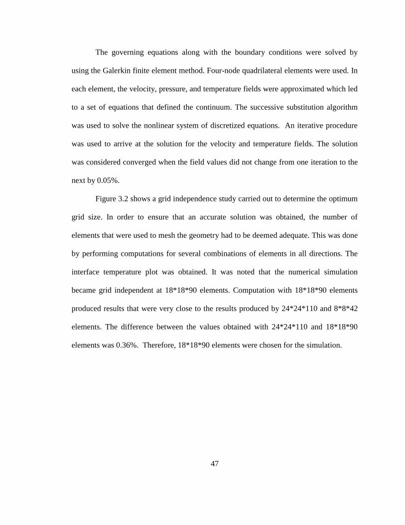
Figure 3.2 shows a grid independence study carried out to determine the optimum

grid size. In order to ensure that an accurate solution was obtained, the number of

elements that were used to mesh the geometry had to be deemed adequate. This was done

by performing computations for several combinations of elements in all directions. The

interface temperature plot was obtained. It was noted that the numerical simulation

became grid independent at 18*18*90 elements. Computation with 18*18*90 elements

produced results that were very close to the results produced by 24*24*110 and 8*8*42

elements. The difference between the values obtained with 24*24*110 and 18*18*90

elements was 0.36%. Therefore, 18*18*90 elements were chosen for the simulation.

48

3.2 Results and Discussion

For all the configurations studied the length of the microchannel (L) was kept

constant at 23 mm. Magnetic field was varied from 2.5T to 10T. Reynolds number used

was between 1000-3000. Height of the gadolinium slab was varied between 1.5 mm to 5

mm and the depth of the channel was varied between 100 μm to 300 μm. The roughness

of microchannel surfaces was neglected in the turbulent analysis.

Figure 3.3 shows the variation of peripheral Nusselt number with dimensionless

axial coordinate for different Reynolds number for magnetic field of 5T. Nusselt number

is seen to be increasing with increase in Reynolds number. The temperature difference

between fluid and solid is more at higher Reynolds number. Thus higher heat transfer

coefficient is obtained at higher Reynolds number. Fluid gets heated as it passes through

the channel. The temperature difference between fluid and solid decreases as one moves

along the length of the channel. Thermal boundary layer grows until fully developed flow

is established. Therefore, the Nusselt number is higher at the entrance and decreases

downstream. The variation is larger at the entrance because of the rapid development of

thermal boundary layer near the leading edge.

Figure 3.4 shows variation of peripheral dimensionless interface temperature for

different Reynolds number and different magnetic fields. The solid-fluid interface

temperature increases as the fluid moves downstream due to the development of thermal

boundary layer starting with the entrance section as the leading edge. Interface

temperature values increase with increase in magnetic field. It can be seen that, as

Reynolds number increases, the interface temperature decreases. For low Reynolds

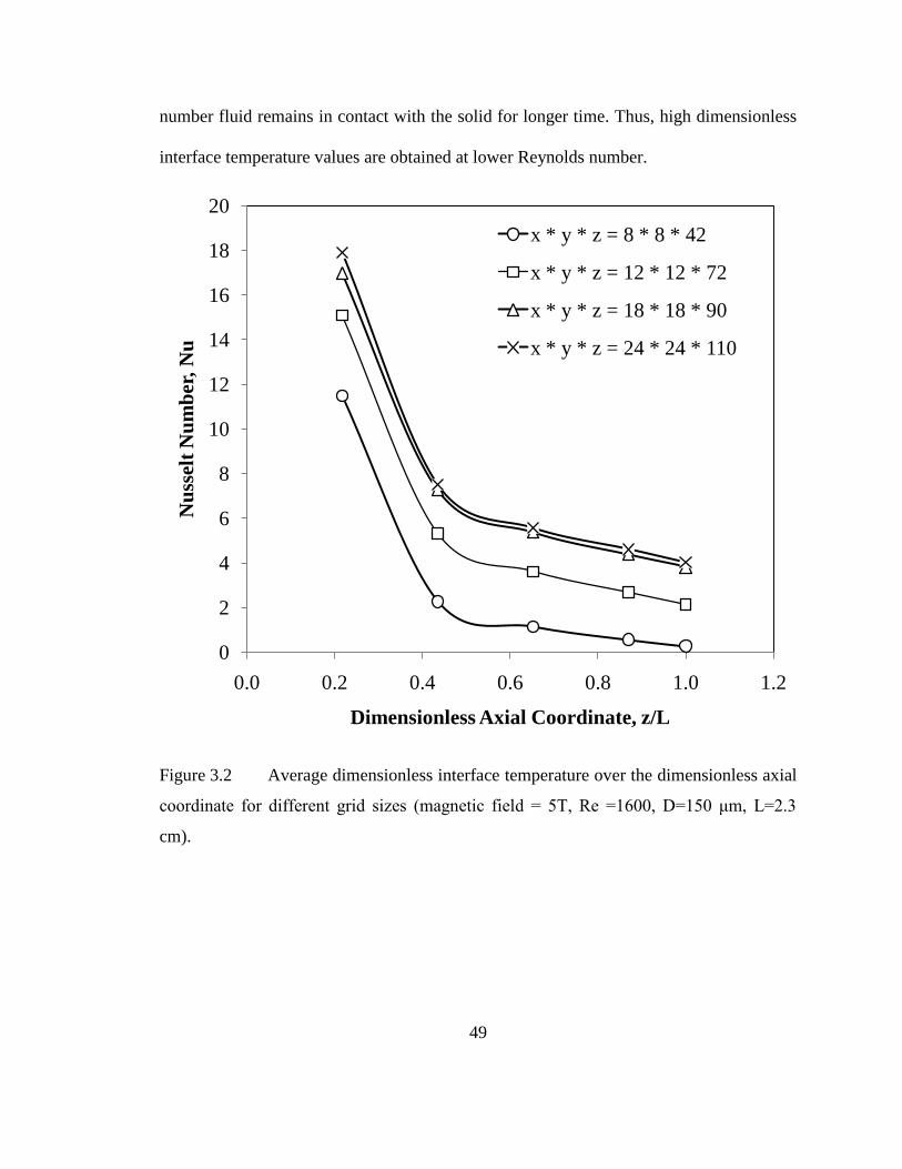
49

number fluid remains in contact with the solid for longer time. Thus, high dimensionless

interface temperature values are obtained at lower Reynolds number.

Figure 3.2 Average dimensionless interface temperature over the dimensionless axial

coordinate for different grid sizes (magnetic field = 5T, Re =1600, D=150 μm, L=2.3

cm).

0

2

4

6

8

10

12

14

16

18

20

0.0 0.2 0.4 0.6 0.8 1.0 1.2

Nu

ssel

t N

um

ber

, N

u

Dimensionless Axial Coordinate, z/L

x * y * z = 8 * 8 * 42

x * y * z = 12 * 12 * 72

x * y * z = 18 * 18 * 90

x * y * z = 24 * 24 * 110

50

Figure 3.3 Variation of peripheral average Nusselt number along the channel

dimensionless axial coordinate for different Reynolds number (Magnetic field = 5T,

D=150 μm, L=2.3 cm).

0

2

4

6

8

10

12

14

16

18

0.0 0.2 0.4 0.6 0.8 1.0 1.2

Nu

ssel

t N

um

ber

, N

u

Dimensionless Axial Coordinate, z/L

Re = 1000

Re = 1600

Re = 2400

Re = 3000

51

Figure 3.4 Variation of peripheral average dimensionless interface temperature along

the channel dimensionless axial coordinate for different Reynolds number and different

magnetic fields (D=150 μm, L=2.3 cm).

0

1

2

3

4

5

6

0.0 0.2 0.4 0.6 0.8 1.0

Dim

ensi

on

less

In

terf

ace

Tem

per

atu

re,

Θ

Dimensionless Axial Coordiate, z/L

2.5T, Re = 1600 2.5T, Re = 2400 2.5T, Re = 3000

5.0T, Re = 1600 5.0T, Re = 2400 5.0T, Re = 3000

10.T, Re = 1600 10.T, Re = 2400 10.T, Re = 3000

52

Figure 3.5 Variation of Nusselt number along the channel dimensionless axial

coordinate for different heat generation rates (Re = 1600, 2400, 3000, D=150 μm, L=2.3

cm).

0

2

4

6

8

10

12

14

16

18

20

0.0 0.2 0.4 0.6 0.8 1.0 1.2

Nu

ssel

t N

um

ber

, N

u

Dimensionless Axial Coordinate, z/L

5T, Re = 1600

5T, Re = 2400

5T, Re = 3000

10T, Re = 1600

10T, Re = 2400

10T, Re = 3000

53

Figure 3.5 shows variation of Nusselt number for different magnetic fields for

Reynolds number of 1600, 2400 and 3000. Nusselt number at a particular cross section in

the channel remains almost the same for different magnetic fields.

Figure 3.6 shows variation of dimensionless interface temperature along the

length of the channel for different thickness of magnetic slab. Reynolds number of fluid

is 1600 and magnetic field is 5T. As shown in figure 1, the slab of magnetic material is

placed on top of the microchannel. As thickness of the slab increases, more heat is

generated in the magnetic material for the same magnetic field. The part of generated

heat is directly dissipated to the working fluid from gadolinium whereas; part is

conducted through the silicon structure and reaches the working fluid. It can be seen that

interface temperature values increase with increase in slab thickness. It was found that

Nusselt number at a particular cross section in the channel remains almost the same for

different thickness of magnetic material slab.

Figure 3.7 shows the dimensionless axial coordinate distribution of the Nusselt

number for different channel depth and constant inlet velocity whose combined effect

changes the Reynolds number. In all these plots, the local Nusselt number is large near

the entrance and decreases downstream due to the development of thermal boundary

layer. For the channel depth > 250 μm, the effect of channel depth on Nusselt number is

less significant. At channel depth lower than 250 μm, the Nusselt number increases with

channel depth over the entire length of the channel. For the channel depth of 250 μm and

300 μm the height of silicon wafer was used were 300μm and 350μm respectively.

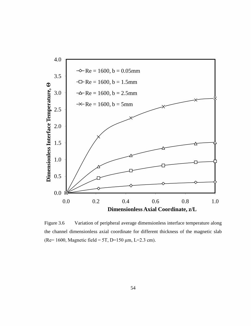
54

Figure 3.6 Variation of peripheral average dimensionless interface temperature along

the channel dimensionless axial coordinate for different thickness of the magnetic slab

(Re= 1600, Magnetic field = 5T, D=150 μm, L=2.3 cm).

0.0

0.5

1.0

1.5

2.0

2.5

3.0

3.5

4.0

0.0 0.2 0.4 0.6 0.8 1.0

Dim

ensi

on

less

In

terf

ace

Tem

per

atu

re,

Θ

Dimensionless Axial Coordinate, z/L

Re = 1600, b = 0.05mm

Re = 1600, b = 1.5mm

Re = 1600, b = 2.5mm

Re = 1600, b = 5mm

55

Figure 3.7 Variation of Nusselt number along the channel dimensionless axial

coordinate for different depths of the channel (Magnetic field =5T, Constant velocity).

0

2

4

6

8

10

12

14

16

18

20

0.0 0.2 0.4 0.6 0.8 1.0

Nu

ssel

t N

um

ber

, N

u

Dimensionless Axial Coordinate, z/L

D = 100 μm

D = 150 μm

D = 200 μm

D = 250 μm

D = 300 μm

56

Figure 3.8 shows the variation of the total average dimensionless interface

temperature of the system for different Reynolds number and different channel depths for

a magnetic field of 5T. It can be seen that as the Reynolds number increases, the average

temperature decreases. A faster moving fluid carries heat at the faster rate, presenting

lower values of average dimensionless interface temperature. For the same Reynolds

number, as the depth of the channel increases, average temperature decreases.

Figure 3.8 Average dimensionless interface temperature numbers with Reynolds

numbers at various channel depths (Magnetic field =5T, 1000 < Re < 3000).

0.0

0.5

1.0

1.5

2.0

2.5

3.0

750 1250 1750 2250 2750 3250

Av

era

ge

Dim

ensi

on

less

In

terf

ace

Tem

per

atu

re,

Θavg

Reynolds Number, Re

D = 161 μm

D = 400 μm

D = 1820 μm

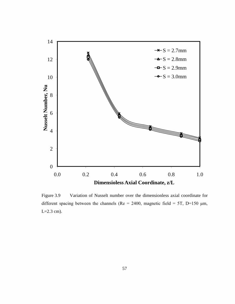
57

Figure 3.9 Variation of Nusselt number over the dimensionless axial coordinate for

different spacing between the channels (Re = 2400, magnetic field = 5T, D=150 μm,

L=2.3 cm).

0

2

4

6

8

10

12

14

0.0 0.2 0.4 0.6 0.8 1.0

Nu

ssel

t N

um

ber

, N

u

Dimensioless Axial Coordinate, z/L

S = 2.7mm

S = 2.8mm

S = 2.9mm

S = 3.0mm

58

Figure 3.9 shows variation of Nusselt number along the length of the channel for

different spacing between the channels. The results show that increasing the solid path

decreases the local Nusselt number along the channel degrading the thermal performance

of the heat sink. The temperature gradient in the solid increases and the average solid

temperature is slightly increased.

Figure 3.10 shows the comparison between the standard convection correlation

and the present simulation model. Nusselt number for laminar flow in a smooth pipe is

calculated by [64],

3/2)/.Pr.(Re4.01

)/.Pr.(Re0668.066.3Nu

LD

LD

h

h

(42)

Nusselt number for turbulent flow in a pipe is calculated by [64],

4.00.8 Pr.0.023ReNu (43)

The values of average Nusselt number for a circular channel with Dh=154μm

were compared to that of the standard convection correlation for a trapezoidal channel

with Dh=154μm. As the average Nusselt number values for circular channel were

compared to those for the trapezoidal channel, there was a difference of 2.23% to 6.52%

between the simulation results and the correlation results.

Figure 3.11 shows variation of dimensionless pressure difference between inlet

and outlet of the channel for different Reynolds numbers. It can be seen that the value of

dimensionless pressure difference between the inlet and outlet of the channel increases as

Reynolds number increases. This is expected because the velocity of the flow increases

with Reynolds number. High velocity fluid creates higher pressure difference between

inlet and outlet. For the same Reynolds number, as the depth of the channel increases,

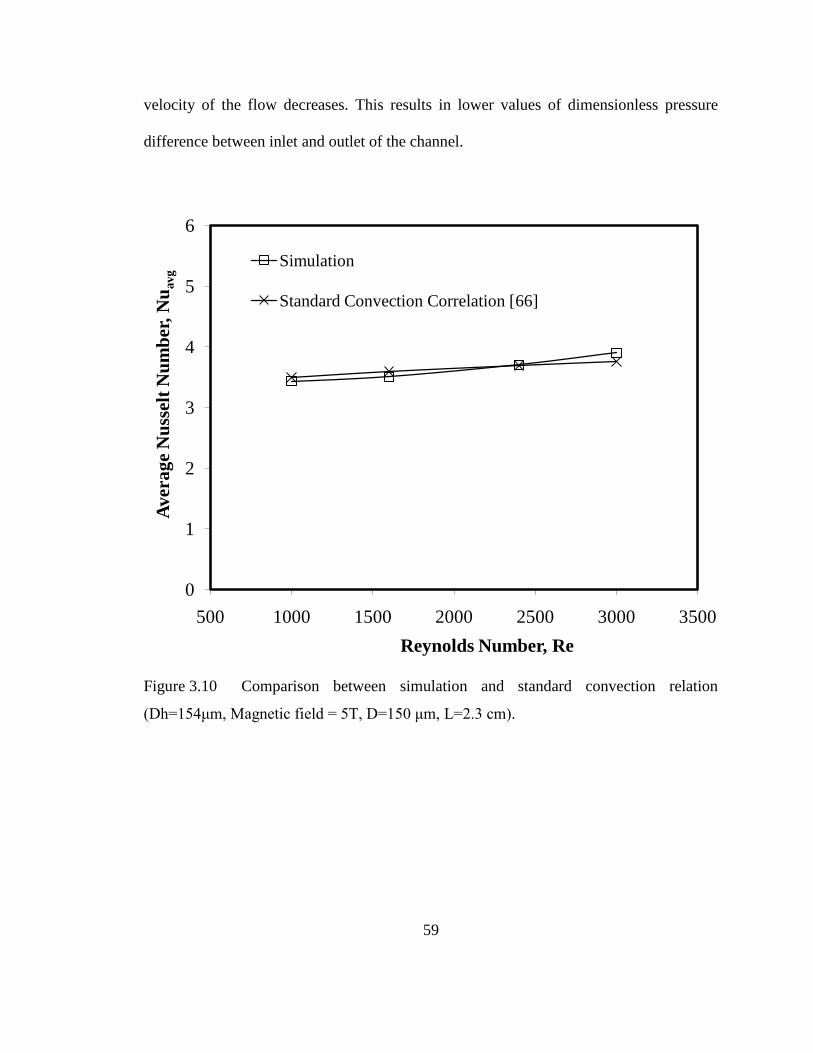
59

velocity of the flow decreases. This results in lower values of dimensionless pressure

difference between inlet and outlet of the channel.

Figure 3.10 Comparison between simulation and standard convection relation

(Dh=154μm, Magnetic field = 5T, D=150 μm, L=2.3 cm).

0

1

2

3

4

5

6

500 1000 1500 2000 2500 3000 3500

Av

era

ge

Nu

ssel

t N

um

ber

, N

uavg

Reynolds Number, Re

Simulation

Standard Convection Correlation [66]

60

Figure 3.11 Variation of dimensionless pressure difference between inlet and outlet of

the channel with Reynolds number (Magnetic field = 5T, L=2.3 cm).

0

2

4

6

8

10

12

14

800 1300 1800 2300 2800 3300

Dim

ensi

on

less

Pre

ssu

re D

iffe

ren

ce, ∆

Pd

Reynolds Number, Re

D = 100 μm

D = 150 μm

D = 200 μm

D = 250 μm

61

Figure 3.12 Variation of the Nusselt numbers for different working fluids (Magnetic

field = 5T, D=150 μm, L=2.3 cm).

0

2

4

6

8

10

12

14

0.00 0.20 0.40 0.60 0.80 1.00 1.20

Nu

ssel

t N

um

ber

, N

u

Dimensionless Axial Coordinate, z/L

Water

Helium

FC-72

62

Figure 3.12 shows variation of average Nusselt number along the dimensionless

axial coordinate of the channel for different working fluids. Thermal conductivity of

water (~ 0.6 W/m-K) is higher than that of helium (~ 0.15 W/m-K) and FC-72 (~ 0.057

W/m-K). This results in better Nusselt number values for water as compared to helium

and FC-72.

Figure 3.13 shows variation of dimensionless pumping power required to pass

the fluid through the channel for different Reynolds numbers. Pumping power is

calculated from volumetric flow rate and pressure difference between inlet and outlet of

the channel. As Reynolds number of fluid increases, the volumetric flow rate and

dimensionless pressure difference increases. For the same Reynolds number, as the depth

of the channel increases, velocity of the flow decreases. Thus, fluid flowing at a higher

velocity requires more pumping power than fluid flowing at a lower velocity.

Figure 3.14 shows two different data of average Nusselt number comparison for a

range of jet Reynolds. This is an attempt to show how close results of simulation from the

present study come close to the experimental data gotten by Wu and Cheng [38]. The

results of the plot were obtained for 200Re40 , L=4cm, Bc=79μm and D=200μm.

The average difference between the results from this plot was 7.17% with a maximum of

13.32%.

63

Figure 3.13 Variation of dimensionless pumping power for different Reynolds

numbers (Magnetic field = 5T, L=2.3 cm).

0.0E+00

5.0E+05

1.0E+06

1.5E+06

2.0E+06

2.5E+06

3.0E+06

750 1250 1750 2250 2750 3250

Dim

ensi

on

less

Pu

mp

ing

Po

wer

, D

p

Reynolds Number, Re

D = 100 μm

D = 150 μm

D = 200 μm

D = 250 μm

64

Figure 3.14 Average Nusselt number comparison with the experimental results

obtained by Wu and Chen [38] under various jet (Magnetic field = 5T, 40 < Re < 200,

D=150 μm, L=4.0 cm).

0

0.3

0.6

0.9

1.2

1.5

1.8

2.1

0 50 100 150 200 250

Av

era

ge

Nu

ssel

t N

um

ber

, N

uavg

Reynolds Number, Re

Simulation

Wu & Chen [8]

65

CHAPTER 4

CONCLUSION

Analysis of impinging jet on a rotating disk was performed. The parameters

utilized include Reynolds number, nozzle height to diameter ratio, rotational speed,

geometry, and fluid property by various Schmidt numbers. The CFD simulation

presented here could be a great tool in understanding the character of a flow in

engineering applications involving jet impingement especially for in etching processes.

The behavior of local and average mass transfer through the dimensionless parameter

Sherwood was investigated using finite element analysis.

The conclusion of this investigation is that the local Sherwood number decreases

with an increasing radius of a rotating or stationary disk which is also the rate of mass

transfer decreasing towards the edge of the disk. An increase in rotational speed of the

disk or Reynolds number at the jet nozzle will lead to an increase in mass transfer rate but

the jet Reynolds has more of an impact. Therefore the results from the investigation for a

low rotational speed of a rotating disk can be approximately equivalent to that of a

stationary disk. Also, with the Reynolds numbers been dealt with, an increase in the

nozzle to target spacing will reduce the mass transfer rate of the species. One of the most

important engineering applications that this study can lend itself is to wet process

equipments and the analysis from this study can be used in design when trying to

determine etching rates.

66

For the microchannel, the simulation was performed by varying the channel

aspect ratio, Reynolds number, heat generation rate and spacing between channels. At a

smaller flow rate outlet temperature increased as the low velocity fluid remained in

contact with the solid for longer time. Heat transfer coefficient and Nusselt number at a

particular cross section in the channel remains almost the same for different heat

generation rates. The peripheral average heat transfer coefficient and Nusselt number

decreases along the length of the channel due to the development of thermal boundary

layer. Large variation in the Nusselt number near the entrance can be attributed to large

growth rate of thermal boundary layer near the leading edge. It is seen that the

temperature in the channel drops down as the hydraulic diameter decreases. For the same

channel, the maximum temperature decreases as the Reynolds number increases. The

pressure drop in the channel increases as the Reynolds number increases. It is also seen

that, as the Reynolds number increases, the power required for pumping the fluid through

the channel increases. Nusselt number increases as the depth of the channel is increased.

For the same channel, Nusselt number increases with Reynolds number.

67

REFERENCES

[1] F. Kreith, J. H. Taylor, and J. P. Chong, “Heat and Mass Transfer from a Rotating

Disk,” Journal of Heat Transfer 81 (1959) 95–104.

[2] V.E. Nakoryakov, B.G. Pokusaev, and E.N. Troyan, “Impingement of an

axisymmetric liquid jet on a barrier,” International Journal of Heat and Mass

Transfer 21 (1978) 1175–1184.

[3] D.T. Chin, and C.H. Tsang, “Mass Transfer to an Impinging Jet Electrode,”

Journal of the Electrochemical Soc. Electrochemical Science and Technology 125

(9) (1978) 1461–1470.

[4] R. Alkire, and J. Ju, “High Speed Selective Electroplating with Impinging Two–

Dimensional Slot Jet Flow,” Journal of the Electrochemical Society 134 (2)

(1987) 294–299.

[5] D.T Chin and M. Agarwal, “Mass Transfer from an Oblique Impinging Slot Jet,”

Journal of the Electrochemical Society 138 (1991) 2643–2650.

68

[6] O.A. Moreno, R.H. Katyl, J.D. Jones, and P.A. Moschak, “Mass Transfer of an

Impinging Jet Confined between Parallel Plates,” IBM J. Res. Develop. 37 (2)

(1993) 143–154.

[7] Y.M. Chen, W.T. Lee, and S.J. Wu, “Heat/Mass Transfer between an Impinging

Jet and Rotating Disk,” Heat and Mass Transfer 34 (1998) 195–201.

[8] T. Pekdemir, and T.W. Davies, “Mass Transfer from Rotating Circular Cylinders

in a Submerged Slot Jet of Air,” International Journal of Heat and Mass Transfer

41 (1998) 3441–3450.

[9] Q. Chen and V. Modi, “Mass transfer in turbulent impinging slot jets,”

International Journal of Heat and Mass Transfer 42 (1999) 762–776.

[10] M. Chen, R. Chalupa, A. C. West, V. Modi, “High Schmidt Mass Transfer in a

Laminar Impinging Slot Jet Flow,” International Journal of Heat and Mass

Transfer 43 (2000) 3907–3915.

[11] J. M. Miranda, and B.L.M. Campos, “Impinging Jets Confined by a Conical Wall

- High Schmidt Mass Transfer Predictions in Laminar Flow,” 44 (2001) 1269–

1284.

69

[12] C.F. Oduoza, “Electrochemical Mass Transfer at a Heated Electrode in a Vertical

Annular Flow Cell,” Chemical Engineering and Processing 43 (2004) 921–928.

[13] M. E. Arzutuğ, S. Yapici, and M.M. Kocakerim, “A comparison of Mass Transfer

between a Plate and Submerged Conventional and Multichannel Impinging Jets,”

International Communications in Heat and Mass Transfer 32 (2005) 842–854.

[14] M.A. Quiroz, U.A. Martinez-Huitle, and C.A. Martinez-Huitle, “Mass Transfer

Measurement in a Parallel Disk Cell Using the Limiting Current Technique,”

Journal Mex. Chem. Soc 49 (3) (2005) 279–283.

[15] G.H. Sedahmed, M.S. Abdo, M.S. Hassan, A.H. Konsowa, “Intensification of

mass transfer controlled processes at the interface between two immiscible liquids

by an axial turbulent submerged jet,” Chemical Engineering and Processing 46

(2007) 10–16.

[16] O.N. Şara, J. Erkmen, S. Yapici, and M. Çopur, “Electrochemical Mass Transfer

between an Impinging Jet and a Rotating Disk in a Confined System,”

International Communications in Heat and Mass Transfer 35 (2008) 289–298.

70

[17] S. K. Hong, D. H. Lee and H. H. Cho, “Heat/Mass transfer measurement on

concave surface in rotating jet impingement,” Journal of Mechanical Science and

Technology 22 (2008) 1952–1958.

[18] S. K. Hong, D.H. Lee, and H.H. Cho, “Effect of Jet Direction on Heat/Mass

Transfer of Rotating Impingement Jet,” Applied Thermal Engineering 29 (2009)

2914–2920.

[19] J. C. Lallave, M. M. Rahman, A. Kumar, “Numerical analysis of heat transfer on

a rotating disk surface under confined liquid jet impingement,” International

Journal of Heat and Fluid Flow 28 (2007) 720–734.

[20] J. C. Lallave, and M. M. Rahman, “Heat Transfer from a Spinning Disk during

Semi–Confined Axial Impingement from a Rotating Nozzle,” International

Journal of Heat and Mass Transfer 51 (2008) 4400–4414.

[21] E.A. Guggenheim, “The Diffusion Coefficient of Sodium Chloride,” Dept. of

Chemistry, The University, Reading 1 (1954) 1048 – 1049.

[22] A.D. Fary, Jr., “The Diffusional Properties of Sodium Hydroxide,” The Institute

of Paper Chemistry, Appleton, Wisconsin, Doctor's Dissertation, January (1966)

73 -74.

71

[23] H. Martin, “Heat and Mass Transfer between Impinging Jets and Solid Surfaces,”

Academic Press, New York, Advances in Heat Transfer 13 (1977) 1–60.

[24] C.O. Popiel, and L. Boguslawski, “Local Heat Transfer from a Rotating Disk in

an Impinging Round Jet,” Journal of Heat Transfer 108 (1986) 357–364.

[25] X.S. Wang, Z. Dagan, and L.M. Jiji, “Heat Transfer between a Circular Free

Impinging Jet and a Solid Surface with Non-uniform Wall Temperature or Wall

Heat Flux–2. Solution for the Boundary Layer Region,” International Journal

Heat Mass Transfer 32 (1989) 1361.

[26] FIDAP Theoretical Manual, Fluid Dynamics International, Inc., Evanston, IL,

(1991).

[27] D.M. Metzger, R.S. Bunker, and G. Bosch, “Transient Liquid Crystal

Measurement of Local Heat Transfer on a Rotating Disk with Jet impingement,”

Turbomachinery 113 (1991) 52–59.

[28] A. Bejan, “Convection Heat Transfer, second edition,” Wiley, New York, 1995

pp. 1–17, pp. 595–600.

72

[29] V.L. Okulovl, S. Martemianov, and T.O. Murakhtina1, “Generalization of the

Leveque Problem for Mass Transfer in Swirling Flows in the Entrance Region of

a Cylindrical Section,” Doklady Physics 47(9) (2002) 685–689. Translated from

Doklady Akademii Nauk 386 (1) (2002) 51–55.

[30] S.Z. Shuja, B.S. Yilbas, M. Rashid, “Confined Swirling Jet Impingement onto an

Adiabatic Wall,” International Journal of Heat and Mass Transfer 46 (2003)

2947–2955.

[31] P.Y. Wu and W.A. Little, “Measurement of friction factors for the flow of gases

in very fine channels used for microminiature Joule-Thomson refrigerators,”

Cryogenics 24 (1983) 273-277.

[32] J.C. Harley, Y. Huang, H.H. Bau and J.N. Zewel, “Gas flow in micro-channels,”

Journal of Fluid Mechanics 284 (1995) 257-274.

[33] K. Chen and Y. Wu, “Thermal analysis and simulation of the microchannel flow

in miniature thermal conductivity detectors,” Sensors and Actuators 79 (2000)

211-218.

[34] W. Qu, G. M. Mala and D. Lee, “Heat transfer for flow in trapezoidal silicon

microchannels,” Int. Journal of Heat and Mass Transfer 21 (2000) 3925-36.

73

[35] M.M. Rahman, “Measurements of heat transfer in microchannel heat sinks,”

International Communications in Heat and Mass Transfer 27 (1) (2000) 495-506.

[36] K.C. Toh, X.Y. Chen and J.C. Chai, “Numerical computation of fluid flow and

heat transfer in microchannels,” International Journal of Heat and Mass Transfer

45 (2002) 5133–5141.

[37] W. Qu and I. Mudawar, “Analysis of three-dimensional heat transfer in micro-

channel heat sinks,” International Journal of Heat and Mass Transfer 45 (2002)

3973–3985.

[38] H.Y. Wu and P. Cheng, “An experimental study of convective heat transfer in

silicon microchannels with different surface conditions,” International Journal of

Heat and Mass Transfer 46 (2003) 2547–2556.

[39] H.Y. Wu and P. Cheng, “Friction factors in smooth trapezoidal silicon micro-

channels with different aspect ratios,” International Journal of Heat and Mass

Transfer 46 (2003) 2519-2525.

[40] J. Li, G.P. Peterson, and P. Cheng, “Three-dimensional analysis of heat transfer in

a micro-heat sink with single phase flow,” International Journal of Heat and Mass

Transfer 47 (2004) 4215–4231.

74

[41] H.L. Mo, Y.X. Zhou, T.Y. Zhu and T.W. Guo, “Forced convection of low

temperature nitrogen gas in rectangular channels with small aspect ratio,”

Cryogenics 44 (2004) 301–307.

[42] W. Owhaib and B. Palm, “Experimental investigation of single-phase convective

heat transfer in circular microchannels,” Experimental Thermal and Fluid

Sciences 28 (2004) 105-110.

[43] H.Y. Wu and P. Cheng, “Boiling instability in parallel silicon microchannels at

different heat flux,” International Journal of Heat and Mass Transfer 47 (2004)

3631-3641.

[44] G.L. Morini, M. Spiga and P. Tartarinic, “The rarefaction effect on the friction

factor of gas flow in microchannels,” Superlattices and Microstructures 35 (2004)

587-599.

[45] Y. Chen and P. Cheng, “Condensation of steam in silicon microchannels,”

International Communications in Heat and Mass Transfer 32 (2005) 175-183.

[46] P. Lee, S. V. Garimella and D. Liu, “Investigation of heat transfer in rectangular

microchannels,” International Journal of Heat and Mass Transfer 48 (2005) 1688–

1704.

75

[47] B. Cao, G. W. Chen and Q. Yuan, “Fully developed laminar flow and heat

transfer in smooth trapezoidal microchannel,” International Communications in

Heat and Mass Transfer 32 (2005) 1211–1220.

[48] G. Hetsroni, A. Mosyak, E. Pogrebnyak and L.P. Yarin, “Heat transfer in micro-

channels: Comparison of experiments with theory and numerical results,”

International Journal of Heat and Mass Transfer 48 (2005) 5580–5601.

[49] L. Zhuo, T. Wen-Quan and H. Ya-Ling, “A numerical study of laminar

convective heat transfer in microchannel with non-circular cross-section,”

International Journal of Thermal Sciences 45 (2006) 1140–1148.

[50] Z. Li, X. Huai, Y. Tao and H. Chen, “Effects of thermal property variations on the

liquid flow and heat transfer in microchannel heat sinks,” Applied Thermal

Engineering 27 (2007) 2803–2814.

[51] A. Husain and K. Kim, “Optimization of a microchannel heat sink with

temperature dependent fluid properties,” Applied Thermal Engineering 28 (2008)

1101–1107.

76

[52] M. M. Rahman, A. A. Gari and S. Shevade, “Heat transfer in circular

microchannels during volumetric heating with magnetic field,” Heat Mass

Transfer 44 (2008) 463–472.

[53] J. Li and C. Kleinstreuer, “Thermal performance of nanofluids flow in

microchannels,” International Journal of Heat and Fluid Flow 29 (2008) 1221–

1232.

[54] K. Hooman, “Heat and fluid flow in a rectangular microchannel filled with a

porous medium,” International Journal of Heat and Mass Transfer 51 (2008)

5804–5810.

[55] M.I. Hasan, A.A. Rageb, M. Yaghoubi and H. Homayoni, “Influence of channel

geometry on the performance of a counter flow microchannel heat exchanger,”

International Journal of Thermal Sciences 48 (2009) 1607–1618.

[56] S. Hsieh and C. Lin, “Convective heat transfer in liquid microchannels with

hydrophobic and hydrophilic surfaces,” International Journal of Heat and Mass

Transfer 52 (2009) 260–270.

77

[57] Y. Chen, C. Zhang, M. Shi and J. Wu, “Three-dimensional numerical simulation

of heat and fluid flow in noncircular microchannel heat sinks,” International

Communications in Heat and Mass Transfer 36 (2009) 917–920.

[58] A.J. DeGregoria, L.J. Feuling, J.F. Laatsch, J.R. Rowe, J.R. Trueblood and A.A.

Wang, “Test results of an active magnetic regenerative refrigerator,” Advances in

Cryogenic Engineering 37 (1992) 875-882.

[59] C. Zimm, A. Jastrab, A. Sternberg, V. Pecharsky, K. Gschneidner, M. Osborne

and I. Anderson, “Description and performance of a near-room temperature

magnetic refrigerator,” Advances in Cryogenic Engineering 43 (1998) 1759-1766.

[60] V.K. Pecharsky and K.A. Gschneidner, “Magnetocaloric effect and magnetic

refrigeration,” Journal of Magnetism and Magnetic Materials 200 (1999) 44-56.

[61] K.K. Ambatipudi and M.M. Rahman, “Analysis of conjugate heat transfer in

microchannel sinks,” Numerical Heat Transfer 37 (A) (2000) 711-731.

[62] Hwang C.B. and Lin C.A., “A low Reynolds number two equation model to

predict thermal fields,” International Journal of Heat and Mass Transfer 42 (2000)

3217-3230.

78

[63] M.N. Ozisik, “Heat Conduction”, 2nd

edition, Wiley (1993) 403-420.

[64] A. Bejan, “Convection Heat Transfer”, 2nd

edition, Interscience (1994) 797-857.

79

APPENDICES

80

Appendix A: FIDAP Code for Analysis of Mass Transfer by Jet Impingement

TITLE( )

JET IMPINGMENT ON ROTATING DISK R1550/W13.09/FLUX

FI-GEN( ELEM = 1, POIN = 1, CURV = 1, SURF = 1, NODE = 0, MEDG = 1,

MLOO = 1,

MFAC = 1, BEDG = 1, SPAV = 1, MSHE = 1, MSOL = 1, COOR = 1, TOLE =

0.0001 )

WINDOW(CHANGE= 1, MATRIX )

1.000000 0.000000 0.000000 0.000000

0.000000 1.000000 0.000000 0.000000

0.000000 0.000000 1.000000 0.000000

0.000000 0.000000 0.000000 1.000000

-10.00000 10.00000 -7.50000 7.50000 -7.50000

7.50000

//ADD POINTS

//POINTS 1,2,3,4,5,6

POINT( ADD, COOR )

0, 0

-0.01, 0

-0.16, 0

-0.16, 0.075

-0.16, 1.5

-0.16, 1.85

-0.01, 1.85

0, 1.85

0, 1.5

0, 0.075

-0.01, 0.075

-0.01, 1.5

-0.01, 1.5

//CONNECT POINTS WITH LINES

//LINES 1,2,3,4,5,6

POINT( SELE, ID )

1

2

3

4

5

6

7

8

9

10

1

CURVE( ADD, LINE )

POINT( SELE, ID )

2

11

12

7

CURVE( ADD, LINE )

POINT( SELE, ID )

12

81

Appendix A: (Continued)

9

CURVE( ADD, LINE )

//USE CORNER POINTS TO MAKE SURFACE

//

POINT( SELE, ID = 1 )

POINT( SELE, ID = 3 )

POINT( SELE, ID = 8 )

POINT( SELE, ID = 6 )

SURFACE( ADD, POIN, ROWW = 2, NOAD )

//CREATE MESH EDGES

//CREATE MESH EDGES

//MEDGE 1,2,3,4,5,6,7,8

CURVE( SELE, ID = 1 )

MEDGE( ADD, SUCC, INTE = 10, RATI = 0, 2RAT = 0, PCEN = 0 )

CURVE( SELE, ID = 2 )

MEDGE( ADD, LSTF, INTE = 20, RATI = 4, 2RAT = 0, PCEN = 0 )

CURVE( SELE, ID = 3 )

MEDGE( ADD, SUCC, INTE = 30, RATI = 0, 2RAT = 0, PCEN = 0 )

CURVE( SELE, ID = 4 )

MEDGE( ADD, SUCC, INTE = 460, RATI = 0, 2RAT = 0, PCEN = 0 )

CURVE( SELE, ID = 5 )

MEDGE( ADD, SUCC, INTE = 10, RATI = 0, 2RAT = 0, PCEN = 0 )

CURVE( SELE, ID = 6 )

MEDGE( ADD, FRST, INTE = 20, RATI = 4, 2RAT = 0, PCEN = 0 )

CURVE( SELE, ID = 7 )

MEDGE( ADD, SUCC, INTE = 10, RATI = 0, 2RAT = 0, PCEN = 0 )

CURVE( SELE, ID = 8 )

MEDGE( ADD, SUCC, INTE = 10, RATI = 0, 2RAT = 0, PCEN = 0 )

CURVE( SELE, ID = 9 )

MEDGE( ADD, SUCC, INTE = 460, RATI = 0, 2RAT = 0, PCEN = 0 )

CURVE( SELE, ID = 10 )

MEDGE( ADD, SUCC, INTE = 30, RATI = 0, 2RAT = 0, PCEN = 0 )

CURVE( SELE, ID = 11 )

MEDGE( ADD, SUCC, INTE = 30, RATI = 0, 2RAT = 0, PCEN = 0 )

CURVE( SELE, ID = 12 )

MEDGE( ADD, SUCC, INTE = 460, RATI = 0, 2RAT = 0, PCEN = 0 )

CURVE( SELE, ID = 13 )

MEDGE( ADD, SUCC, INTE = 10, RATI = 0, 2RAT = 0, PCEN = 0 )

CURVE( SELE, ID = 14 )

MEDGE( ADD, SUCC, INTE = 10, RATI = 0, 2RAT = 0, PCEN = 0 )

//MAKE A LOOP OUT THE LINES

//LOOP 1

CURVE( SELE, ID )

1

11

12

14

9

10

MLOOP( ADD, MAP, VISI, NOSH, EDG1 = 1, EDG2 = 2, EDG3 = 1, EDG4 = 2 )

//LOOP 2

CURVE( SELE, ID )

82

Appendix A: (Continued)

14

13

7

8

MLOOP( ADD, MAP, VISI, NOSH, EDG1 = 1, EDG2 = 1, EDG3 = 1, EDG4 = 1 )

//LOOP 3

CURVE( SELE, ID )

2

3

4

5

6

13

12

11

MLOOP( ADD, MAP, VISI, NOSH, EDG1 = 1, EDG2 = 3, EDG3 = 1, EDG4 = 3 )

//ADD A FACE

//FACE 1

SURFACE( SELE, ID = 1 )

MLOOP( SELE, ID = 1 )

MFACE( ADD )

//FACE 2

SURFACE( SELE, ID = 1 )

MLOOP( SELE, ID = 2 )

MFACE( ADD )

//FACE 3

SURFACE( SELE, ID = 1 )

MLOOP( SELE, ID = 3 )

MFACE( ADD )

//ADD MESH

//MESH 1

MFACE( SELE, ID = 1 )

ELEMENT( SETD, QUAD, NODE = 4 )

MFACE( MESH, MAP, NOSM, ENTI = "nickel" )

//MESH 2

MFACE( SELE, ID = 2 )

ELEMENT( SETD, QUAD, NODE = 4 )

MFACE( MESH, MAP, NOSM, ENTI = "water" )

//MESH 3

MFACE( SELE, ID = 3 )

ELEMENT( SETD, QUAD, NODE = 4 )

MFACE( MESH, MAP, NOSM, ENTI = "water" )

//MESH MAP ELEMENT ID

//

ELEMENT( SETD, EDGE, NODE = 2 )

MEDGE( SELE, ID = 1 )

MEDGE( MESH, MAP, ENTI = "outside" )

MEDGE( SELE, ID = 2 )

MEDGE( MESH, MAP, ENTI = "axis" )

MEDGE( SELE, ID = 3 )

MEDGE( MESH, MAP, ENTI = "inflow" )

MEDGE( SELE, ID = 4 )

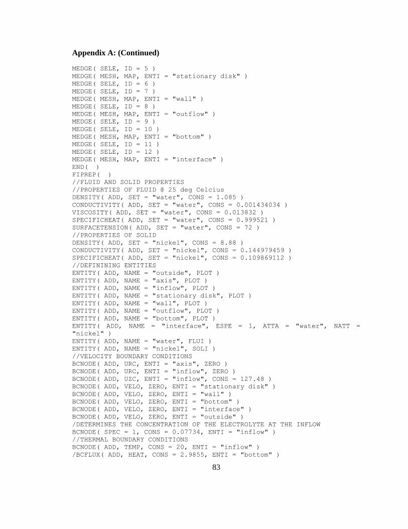
83

Appendix A: (Continued)

MEDGE( SELE, ID = 5 )

MEDGE( MESH, MAP, ENTI = "stationary disk" )

MEDGE( SELE, ID = 6 )

MEDGE( SELE, ID = 7 )

MEDGE( MESH, MAP, ENTI = "wall" )

MEDGE( SELE, ID = 8 )

MEDGE( MESH, MAP, ENTI = "outflow" )

MEDGE( SELE, ID = 9 )

MEDGE( SELE, ID = 10 )

MEDGE( MESH, MAP, ENTI = "bottom" )

MEDGE( SELE, ID = 11 )

MEDGE( SELE, ID = 12 )

MEDGE( MESH, MAP, ENTI = "interface" )

END( )

FIPREP( )

//FLUID AND SOLID PROPERTIES

//PROPERTIES OF FLUID @ 25 deg Celcius

DENSITY( ADD, SET = "water", CONS = 1.085 )

CONDUCTIVITY( ADD, SET = "water", CONS = 0.001434034 )

VISCOSITY( ADD, SET = "water", CONS = 0.013832 )

SPECIFICHEAT( ADD, SET = "water", CONS = 0.999521 )

SURFACETENSION( ADD, SET = "water", CONS = 72 )

//PROPERTIES OF SOLID

DENSITY( ADD, SET = "nickel", CONS = 8.88 )

CONDUCTIVITY( ADD, SET = "nickel", CONS = 0.144979459 )

SPECIFICHEAT( ADD, SET = "nickel", CONS = 0.109869112 )

//DEFININING ENTITIES

ENTITY( ADD, NAME = "outside", PLOT )

ENTITY( ADD, NAME = "axis", PLOT )

ENTITY( ADD, NAME = "inflow", PLOT )

ENTITY( ADD, NAME = "stationary disk", PLOT )

ENTITY( ADD, NAME = "wall", PLOT )

ENTITY( ADD, NAME = "outflow", PLOT )

ENTITY( ADD, NAME = "bottom", PLOT )

ENTITY( ADD, NAME = "interface", ESPE = 1, ATTA = "water", NATT =

"nickel" )

ENTITY( ADD, NAME = "water", FLUI )

ENTITY( ADD, NAME = "nickel", SOLI )

//VELOCITY BOUNDARY CONDITIONS

BCNODE( ADD, URC, ENTI = "axis", ZERO )

BCNODE( ADD, URC, ENTI = "inflow", ZERO )

BCNODE( ADD, UZC, ENTI = "inflow", CONS = 127.48 )

BCNODE( ADD, VELO, ZERO, ENTI = "stationary disk" )

BCNODE( ADD, VELO, ZERO, ENTI = "wall" )

BCNODE( ADD, VELO, ZERO, ENTI = "bottom" )

BCNODE( ADD, VELO, ZERO, ENTI = "interface" )

BCNODE( ADD, VELO, ZERO, ENTI = "outside" )

/DETERMINES THE CONCENTRATION OF THE ELECTROLYTE AT THE INFLOW

BCNODE( SPEC = 1, CONS = 0.07734, ENTI = "inflow" )

//THERMAL BOUNDARY CONDITIONS

BCNODE( ADD, TEMP, CONS = 20, ENTI = "inflow" )

/BCFLUX( ADD, HEAT, CONS = 2.9855, ENTI = "bottom" )

84

Appendix A: (Continued)

//MASS FLUX

BCFLUX( ADD, SPEC = 1, ENTI = "interface", CONS = 0.0001624 )

//THIS BOUNDARY CONDITION IS EQUIVALENT TO 1436 RPM

BCNODE( UTHE, POLY = 1, ENTI = "nickel" )

0, 13.09, 0, 1, 0

BODYFORCE( ADD, CONS, FX = 981, FY = 0, FZ = 0 )

PRESSURE( ADD, MIXE = 1e-11, DISC )

DATAPRINT( ADD, CONT )

EXECUTION( ADD, NEWJ ) PRINTOUT( ADD, NONE, BOUN )

OPTIONS( ADD, UPWI )

UPWINDING( ADD, STRE )

PROBLEM( ADD, CYLI, INCO, TRAN, LAMI, NONL, NEWT, MOME, ISOT, FIXE,

SING,

SPEC = 1 )

/PROBLEM( ADD, CYLI, INCO, TRAN, LAMI, NONL, NEWT, MOME, ENERGY, FIXE,

SING, SPECIES = 1 )

SOLUTION( ADD, N.R. = 50, KINE = 20, VELC = 0.0001, RESC = 0.0001 )

TIMEINTEGRATION( ADD, BACK, NSTE = 301, TSTA = 0, DT = 1e-05, VARI,

WIND = 1,

NOFI = 10 )

POSTPROCESS( NBLO = 2 )

1, 95, 47

95, 301, 1

CLIPPING( ADD, MINI )

0, 0, 0, 0, 20, 0, 0, 0, 0.07734

ICNODE( ADD, URC, ENTI = "water", CONS = 10 )

ICNODE( ADD, UTHE, ENTI = "water", CONS = 5 )

//ADDED FOR MASS TRANSFER AND DIFFUSION COEFFICIENTS RESPECTIVELY

//SPTRANSFER( ADD, SET = 1, CONSTANT = 0.0000002029, POWER=1.0,

TEMPERATURE )

DIFFUSIVITY( SET = 1, CONS = 5.508e-06, ISOT, TEMP )

CAPACITY( CONS = 1 )

END( )

CREATE( FISO )

RUN( FISOLV, BACK, AT = "", TIME = "NOW", COMP )

/ File closed at Fri Aug 7 18:01:35 2009.

/ File opened for append Fri Aug 7 18:48:23 2009.

FIPOST( )

TIMESTEP( STEP = -1 )

TIMESTEP( STEP = 95 )

LINE( SPEC = 1, ENTI = "interface" )

END( )

END( )

FIPOST( )

DEVICE( POST, FILE = "MESHPLOT" )

MESH( )

END( )

END( )

FIPOST( )

DEVICE( POST, FILE = "VECTPLOT" )

VECTOR( VELO, FACT = 50 )

85

Appendix A: (Continued)

END( )

END( )

/ File closed at Sun Aug 23 19:15:27 2009.

/ File opened for append Mon Aug 24 01:39:20 2009.

FIPOST( )

DEVICE( POST, FILE = "VECT3PLOT" )

VECTOR( VELO, FACT = 50 ) END( )

FIPOST( )

DEVICE( POST, FILE = "STRM3PLOT" )

CONTOUR( STRE, AUTO = 40 )

END( )

86

Appendix B: FIDAP Code for Fluid Flow and Heat Transfer in a Composite

Trapezoidal Microchannel

TITLE( )

MICROCHANNEL

FI-GEN( ELEM = 1, POIN = 1, CURV = 1, SURF = 1, NODE = 0, MEDG = 1,

MLOO = 1,

MFAC = 1, BEDG = 1, SPAV = 1, MSHE = 1, MSOL = 1, COOR = 1, TOLE =

0.0001 )

WINDOW(CHANGE= 1, MATRIX )

1.000000 0.000000 0.000000 0.000000

0.000000 1.000000 0.000000 0.000000

0.000000 0.000000 1.000000 0.000000

0.000000 0.000000 0.000000 1.000000

-10.00000 10.00000 -7.50000 7.50000 -7.50000

7.50000

/^^^^^^^^^^^^^^^^^^^^^^^^^^^^^^^^^^^^^^^^^^^^^^^^^^^^^^^^^^^^^^^^^^^

/ COORDINATES FOR POINTS

/^^^^^^^^^^^^^^^^^^^^^^^^^^^^^^^^^^^^^^^^^^^^^^^^^^^^^^^^^^^^^^^^^^^^

POINT( ADD, COOR )

0, 0, 0

0.305, 0, 0

0.305, 0.01, 0

0.305, 0.025, 0

0.305, 0.525, 0

0, 0.525, 0

0, 0.025, 0

0, 0.01, 0

0.3006, 0.01, 0

0.29, 0.025, 0

0, 0.01, 2.3

0.305, 0.025, 2.3

0, 0, 0.5

0.305, 0, 0.5

0.305, 0.01, 0.5

0.305, 0.025, 0.5

0.305, 0.525, 0.5

0, 0.525, 0.5

0, 0.025, 0.5

0, 0.01, 0.5

0.3006, 0.01, 0.5

0.29, 0.025, 0.5

0, 0, 1

0.305, 0, 1

0.305, 0.01, 1

0.305, 0.025, 1

0.305, 0.525, 1

0, 0.525, 1

0, 0.025, 1

0, 0.01, 1

0.3006, 0.01, 1

0.29, 0.025, 1

0, 0, 1.5

0.305, 0, 1.5

87

Appendix B: (Continued)

0.305, 0.01, 1.5

0.305, 0.025, 1.5

0.305, 0.525, 1.5

0, 0.525, 1.5

0, 0.025, 1.5

0, 0.01, 1.5

0.3006, 0.01, 1.5

0.29, 0.025, 1.5

0, 0, 2

0.305, 0, 2

0.305, 0.01, 2

0.305, 0.025, 2

0.305, 0.525, 2

0, 0.525, 2

0, 0.025, 2

0, 0.01, 2

0.3006, 0.01, 2

0.29, 0.025, 2

0, 0, 2.3

0.305, 0, 2.3

0.305, 0.01, 2.3

0.305, 0.025, 2.3

0.305, 0.525, 2.3

0, 0.525, 2.3

0, 0.025, 2.3

0, 0.01, 2.3

0.3006, 0.01, 2.3

0.29, 0.025, 2.3

/^^^^^^^^^^^^^^^^^^^^^^^^^^^^^^^^^^^^^^^^^^^^^^^^^^^^^^^^^^^^^^^^^^^

/ CONNECTING POINTS WITH LINES

/^^^^^^^^^^^^^^^^^^^^^^^^^^^^^^^^^^^^^^^^^^^^^^^^^^^^^^^^^^^^^^^^^^^

//PART ONE

/LINES 1 - 8

POINT( SELE, ID )

1

2

3

4

5

6

7

8

1

CURVE( ADD, LINE )

/LINES 9

POINT( SELE, ID )

9

3

CURVE( ADD, LINE )

/LINES 10 - 11

POINT( SELE, ID )

7

88

Appendix B: (Continued)

10

4

CURVE( ADD, LINE )

/LINES 12

POINT( SELE, ID )

9

10

CURVE( ADD, LINE )

/LINES 13

POINT( SELE, ID )

8

9

CURVE( ADD, LINE )

/LINES 14

POINT( SELE, ID )

8

11

CURVE( ADD, LINE )

/LINES 15

POINT( SELE, ID )

4

12

CURVE( ADD, LINE )

//PART TWO

/LINES 16 - 23

POINT( SELE, ID )

13

14

15

16

17

18

19

20

13

CURVE( ADD, LINE )

/LINES 24

POINT( SELE, ID )

21

15

CURVE( ADD, LINE )

/LINES 25 - 26

POINT( SELE, ID )

19

22

16

CURVE( ADD, LINE )

/LINES 27

POINT( SELE, ID )

21

22

CURVE( ADD, LINE )

89

Appendix B: (Continued)

/LINES 28

POINT( SELE, ID )

20

21

CURVE( ADD, LINE )

//PART THREE

/LINES 29 - 36

POINT( SELE, ID )

23

24

25

26

27

28

29

30

23

CURVE( ADD, LINE )

/LINES 37

POINT( SELE, ID )

31

25

CURVE( ADD, LINE )

/LINES 38 - 39

POINT( SELE, ID )

29

32

26

CURVE( ADD, LINE )

/LINES 40

POINT( SELE, ID )

31

32

CURVE( ADD, LINE )

/LINES 41

POINT( SELE, ID )

30

31

CURVE( ADD, LINE )

//PART FOUR

/LINES 42 - 49

POINT( SELE, ID )

33

34

35

36

37

38

39

40

33

CURVE( ADD, LINE )

90

Appendix B: (Continued)

/LINES 50

POINT( SELE, ID )

41

35

CURVE( ADD, LINE )

/LINES 51

POINT( SELE, ID )

39

42

36

CURVE( ADD, LINE )

/LINES 53

POINT( SELE, ID )

41

42

CURVE( ADD, LINE )

/LINES 54

POINT( SELE, ID )

40

41

CURVE( ADD, LINE )

//PART FIVE

/LINES 55 - 62

POINT( SELE, ID )

43

44

45

46

47

48

49

50

43

CURVE( ADD, LINE )

/LINES 63

POINT( SELE, ID )

51

45

CURVE( ADD, LINE )

/LINES 64

POINT( SELE, ID )

49

52

46

CURVE( ADD, LINE )

/LINES 66

POINT( SELE, ID )

51

52

CURVE( ADD, LINE )

/LINES 67

POINT( SELE, ID )

91

Appendix B: (Continued)

50

51

CURVE( ADD, LINE )

//PART SIX

/LINES 68 - 75

POINT( SELE, ID )

53

54

55

56

57

58

59

60

53

CURVE( ADD, LINE )

/LINES 76

POINT( SELE, ID )

61

55

CURVE( ADD, LINE )

/LINES 77

POINT( SELE, ID )

59

62

56

CURVE( ADD, LINE )

/LINES 79

POINT( SELE, ID )

61

62

CURVE( ADD, LINE )

/LINES 80

POINT( SELE, ID )

60

61

CURVE( ADD, LINE )

///////////////////////////////////////////////////////////////////////

/

//CREATING SURFACES

CURVE( SELE, ID )

1

2

3

4

5

6

7

8

SURFACE( ADD, WIRE, EDG1 = 1, EDG2 = 3, EDG3 = 1, EDG4 = 3 )

CURVE( SELE, ID )

16

92

Appendix B: (Continued)

17

18

19

20

21

22

23

SURFACE( ADD, WIRE, EDG1 = 1, EDG2 = 3, EDG3 = 1, EDG4 = 3 )

CURVE( SELE, ID )

29

30

31

32

33

34

35

36

SURFACE( ADD, WIRE, EDG1 = 1, EDG2 = 3, EDG3 = 1, EDG4 = 3 )

CURVE( SELE, ID )

42

43

44

45

46

47

48

49

SURFACE( ADD, WIRE, EDG1 = 1, EDG2 = 3, EDG3 = 1, EDG4 = 3 )

CURVE( SELE, ID )

55

56

57

58

59

60

61

62

SURFACE( ADD, WIRE, EDG1 = 1, EDG2 = 3, EDG3 = 1, EDG4 = 3 )

CURVE( SELE, ID )

68

69

70

71

72

73

74

75

SURFACE( ADD, WIRE, EDG1 = 1, EDG2 = 3, EDG3 = 1, EDG4 = 3 )

///////////////////////////////////////////////////////////////////////

///

//CREATING MESH EDGES

CURVE( SELE, ID = 1 )

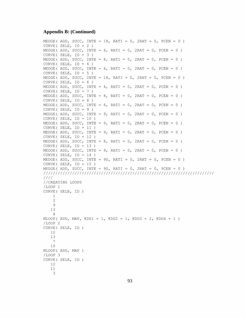
93

Appendix B: (Continued)

MEDGE( ADD, SUCC, INTE = 18, RATI = 0, 2RAT = 0, PCEN = 0 )

CURVE( SELE, ID = 2 )

MEDGE( ADD, SUCC, INTE = 6, RATI = 0, 2RAT = 0, PCEN = 0 )

CURVE( SELE, ID = 3 )

MEDGE( ADD, SUCC, INTE = 8, RATI = 0, 2RAT = 0, PCEN = 0 )

CURVE( SELE, ID = 4 )

MEDGE( ADD, SUCC, INTE = 4, RATI = 0, 2RAT = 0, PCEN = 0 )

CURVE( SELE, ID = 5 )

MEDGE( ADD, SUCC, INTE = 18, RATI = 0, 2RAT = 0, PCEN = 0 )

CURVE( SELE, ID = 6 )

MEDGE( ADD, SUCC, INTE = 4, RATI = 0, 2RAT = 0, PCEN = 0 )

CURVE( SELE, ID = 7 )

MEDGE( ADD, SUCC, INTE = 8, RATI = 0, 2RAT = 0, PCEN = 0 )

CURVE( SELE, ID = 8 )

MEDGE( ADD, SUCC, INTE = 6, RATI = 0, 2RAT = 0, PCEN = 0 )

CURVE( SELE, ID = 9 )

MEDGE( ADD, SUCC, INTE = 9, RATI = 0, 2RAT = 0, PCEN = 0 )

CURVE( SELE, ID = 10 )

MEDGE( ADD, SUCC, INTE = 9, RATI = 0, 2RAT = 0, PCEN = 0 )

CURVE( SELE, ID = 11 )

MEDGE( ADD, SUCC, INTE = 9, RATI = 0, 2RAT = 0, PCEN = 0 )

CURVE( SELE, ID = 12 )

MEDGE( ADD, SUCC, INTE = 8, RATI = 0, 2RAT = 0, PCEN = 0 )

CURVE( SELE, ID = 13 )

MEDGE( ADD, SUCC, INTE = 9, RATI = 0, 2RAT = 0, PCEN = 0 )

CURVE( SELE, ID = 14 )

MEDGE( ADD, SUCC, INTE = 90, RATI = 0, 2RAT = 0, PCEN = 0 )

CURVE( SELE, ID = 15 )

MEDGE( ADD, SUCC, INTE = 90, RATI = 0, 2RAT = 0, PCEN = 0 )

///////////////////////////////////////////////////////////////////////

////

//CREATING LOOPS

/LOOP 1

CURVE( SELE, ID )

1

2

9

13

8

MLOOP( ADD, MAP, EDG1 = 1, EDG2 = 1, EDG3 = 2, EDG4 = 1 )

/LOOP 2

CURVE( SELE, ID )

12

13

7

10

MLOOP( ADD, MAP )

/LOOP 3

CURVE( SELE, ID )

12

11

3

94

Appendix B: (Continued)

9

MLOOP( ADD, MAP )

/LOOP 4

CURVE( SELE, ID )

4

5

6

10

11

MLOOP( ADD, MAP, EDG1 = 1, EDG2 = 1, EDG3 = 1, EDG4 = 2 )

///////////////////////////////////////////////////////////////////////

//////

//CREATING FACE FOR MESH

SURFACE( SELE, ID = 1 )

MLOOP( SELE, ID = 1 )

MFACE( ADD )

//CREATING FACE FOR MESH

SURFACE( SELE, ID = 1 )

MLOOP( SELE, ID = 2 )

MFACE( ADD )

//CREATING FACE FOR MESH

SURFACE( SELE, ID = 1 )

MLOOP( SELE, ID = 3 )

MFACE( ADD )

//CREATING FACE FOR MESH

SURFACE( SELE, ID = 1 )

MLOOP( SELE, ID = 4 )

MFACE( ADD )

///////////////////////////////////////////////////////////////////////

/////

//CREATING SOLID FOR THE MESH

MFACE( SELE, ID = 1 )

CURVE( SELE, ID = 14 )

MSOLID( PROJ )

MFACE( SELE, ID = 2 )

CURVE( SELE, ID = 14 )

MSOLID( PROJ )

MFACE( SELE, ID = 3 )

CURVE( SELE, ID = 15 )

MSOLID( PROJ )

MFACE( SELE, ID = 4 )

CURVE( SELE, ID = 15 )

MSOLID( PROJ )

///////////////////////////////////////////////////////////////////////

/////

//CREATION OF THE MESH AND ASSIGNING CONTINUOUS ENTITIES

MSOLID( SELE, ID = 1 )

ELEMENT( SETD, BRIC, NODE = 8 )

MSOLID( MESH, MAP, ENTI = "SILICON" )

MSOLID( SELE, ID = 2 )

ELEMENT( SETD, BRIC, NODE = 8 )

MSOLID( MESH, MAP, ENTI = "SILICON" )

95

Appendix B: (Continued)

MSOLID( SELE, ID = 3 )

ELEMENT( SETD, BRIC, NODE = 8 )

MSOLID( MESH, MAP, ENTI = "FLUID" )

MSOLID( SELE, ID = 4 )

ELEMENT( SETD, BRIC, NODE = 8 )

MSOLID( MESH, MAP, ENTI = "GADOLINIUM" )

///////////////////////////////////////////////////////////////////////

////

//ASSIGNING ENTITIES TO VARIOUS BOUNDARIES

MFACE( SELE, ID = 3 )

MFACE( MESH, MAP, ENTI = "Fin" )

MFACE( SELE, ID = 15 )

MFACE( MESH, MAP, ENTI = "Fout" )

/MFACE( SELE, ID = 12 )

/MFACE( SELE, ID = 17 )

/MFACE( MESH, MAP, ENTI = "HF" )

MFACE( SELE, ID = 8 )

MFACE( MESH, MAP, ENTI = "Fbot" )

MFACE( SELE, ID = 17 )

MFACE( MESH, MAP, ENTI = "Ftop" )

MFACE( SELE, ID = 16 )

MFACE( MESH, MAP, ENTI = "Faxis" )

MFACE( SELE, ID = 14 )

MFACE( MESH, MAP, ENTI = "Fleft" )

MFACE( SELE, ID = 6 )

MFACE( MESH, MAP, ENTI = "Sbot" )

MFACE( SELE, ID = 7 )

MFACE( MESH, MAP, ENTI = "Saxis" )

MFACE( SELE, ID = 19 )

MFACE( MESH, MAP, ENTI = "Gaxis" )

MFACE( SELE, ID = 20 )

MFACE( MESH, MAP, ENTI = "Gtop" )

MFACE( SELE, ID = 21 )

MFACE( MESH, MAP, ENTI = "Gleft" )

MFACE( SELE, ID = 13 )

MFACE( MESH, MAP, ENTI = "Sleft1" )

MFACE( SELE, ID = 10 )

MFACE( MESH, MAP, ENTI = "Sleft2" )

MEDGE( SELE, ID = 23 )

MEDGE( MESH, MAP, ENTI = "RTedge" )

MEDGE( SELE, ID = 22 )

MEDGE( MESH, MAP, ENTI = "RBedge" )

MEDGE( SELE, ID = 24 )

MEDGE( MESH, MAP, ENTI = "LTedge" )

MEDGE( SELE, ID = 21 )

MEDGE( MESH, MAP, ENTI = "LBedge" )

END( )

FIPREP( )

///////////////////////////////////////////////////////////////////////

////

//PROPERTY OF SILICON

CONDUCTIVITY( ADD, SET = "SILICON", CONS = 0.29637, ISOT )

96

Appendix B: (Continued)

DENSITY( ADD, SET = "SILICON", CONS = 2.329 )

SPECIFICHEAT( ADD, SET = "SILICON", CONS = 0.16778 )

//PROPERTY OF FLUID

CONDUCTIVITY( ADD, SET = "FLUID", CONS = 0.0014435, ISOT )

DENSITY( ADD, SET = "FLUID", CONS = 0.9974 )

SPECIFICHEAT( ADD, SET = "FLUID", CONS = 0.9988 )

VISCOSITY( ADD, SET = "FLUID", CONS = 0.0098 )

//PROPERTY OF GADOLINIUM

CONDUCTIVITY( ADD, SET = "GADOLINIUM", CONS = 0.0250956, ISOT )

DENSITY( ADD, SET = "GADOLINIUM", CONS = 7.895 )

SPECIFICHEAT( ADD, SET = "GADOLINIUM", CONS = 0.054971 )

///////////////////////////////////////////////////////////////////////

/////

//DEFINING ENTITIES

ENTITY( ADD, NAME = "SILICON", SOLI )

ENTITY( ADD, NAME = "GADOLINIUM", SOLI )

ENTITY( ADD, NAME = "FLUID", FLUI )

ENTITY( ADD, NAME = "Fin", PLOT )

ENTITY( ADD, NAME = "Fout", PLOT )

/ENTITY( ADD, NAME = "HF", PLOT, ATTA = "FLUID", NATTA = "GADOLINIUM" )

ENTITY( ADD, NAME = "Fbot", PLOT, ATTA = "FLUID", NATT = "SILICON" )

ENTITY( ADD, NAME = "Ftop", PLOT, ATTA = "FLUID", NATT = "GADOLINIUM" )

ENTITY( ADD, NAME = "Faxis", PLOT )

ENTITY( ADD, NAME = "Fleft", PLOT, ATTA = "FLUID", NATT = "SILICON" )

ENTITY( ADD, NAME = "Sbot", PLOT )

ENTITY( ADD, NAME = "Saxis", PLOT )

ENTITY( ADD, NAME = "Gaxis", PLOT )

ENTITY( ADD, NAME = "Gtop", PLOT )

ENTITY( ADD, NAME = "Gleft", PLOT )

ENTITY( ADD, NAME = "Sleft1", PLOT )

ENTITY( ADD, NAME = "Sleft2", PLOT )

ENTITY( ADD, NAME = "RTedge", PLOT )

ENTITY( ADD, NAME = "RBedge", PLOT )

ENTITY( ADD, NAME = "LTedge", PLOT )

ENTITY( ADD, NAME = "LBedge", PLOT )

///////////////////////////////////////////////////////////////////////

/////

//INITIAL AND BOUNDARY CONDITION

BCNODE( ADD, UX, ENTI = "Fin", ZERO )

BCNODE( ADD, UY, ENTI = "Fin", ZERO )

BCNODE( ADD, UZ, ENTI = "Fin", CONS = 1425.34 )

BCNODE( ADD, TEMP, ENTI = "Fin", CONS = 20 )

BCNODE( ADD, VELO, ENTI = "Fbot", ZERO )

BCNODE( ADD, VELO, ENTI = "Ftop", ZERO )

BCNODE( ADD, VELO, ENTI = "Fleft", ZERO )

BCNODE( ADD, UX, ENTI = "Faxis", ZERO )

/BCFLUX( ADD, HEAT, ENTI = "HF", CONS = 14.49 )

BCFLUX( ADD, HEAT, ENTI = "Sbot", CONS = 0 )

BCFLUX( ADD, HEAT, ENTI = "Saxis", CONS = 0 )

BCFLUX( ADD, HEAT, ENTI = "Gaxis", CONS = 0 )

BCFLUX( ADD, HEAT, ENTI = "Gtop", CONS = 0 )

BCFLUX( ADD, HEAT, ENTI = "Gleft", CONS = 0 )

97

Appendix B: (Continued)

BCFLUX( ADD, HEAT, ENTI = "Sleft1", CONS = 0 )

BCFLUX( ADD, HEAT, ENTI = "Sleft2", CONS = 0 )

SOURCE( ADD, HEAT, CONS = 6.080715996, ENTI = "GADOLINIUM" )

ICNODE( ADD, TEMP, CONS = 20, ENTI = "SILICON" )

ICNODE( ADD, TEMP, CONS = 20, ENTI = "GADOLINIUM" )

ICNODE( ADD, TEMP, CONS = 20, ENTI = "FLUID" )

///////////////////////////////////////////////////////////////////////

//

//IF THE FLOW IT TURBULENT AND K-E MODEL IS USED, ADD THE FOLLOWING

//LINES OF CODES

/VISCOSITY( ADD, SET = "FLUID", TWO-, CONS = 0.0098 )

/ICNODE( KINE, CONS = 0.003, ALL )

/ICNODE( DISS, CONS = 0.00045, ALL )

/BCNODE( KINE, CONS = 0.001, ENTI = "Fin" )

/BCNODE( DISS, CONS = 0.00045, ENTI = "Fin" )

///////////////////////////////////////////////////////////////////////

////

//EXECUTION COMMANDS

DATAPRINT( ADD, CONT )

EXECUTION( ADD, NEWJ )

PRINTOUT( ADD, NONE, BOUN )

PROBLEM( ADD, 3-D, INCO, STEA, LAMI, NONL, NEWT, MOME, ENER, FIXE, SING

)

SOLUTION( ADD, SEGR = 10, PREC = 21, ACCF = 0, PPRO )

END( )

CREATE( FISO )

RUN( FISOLV, BACK, AT = "", TIME = "NOW", COMP )

END( )

FIPOST( )

PRINT( PRES, POIN, FILE = "comb.txt", SCRE )

324

0.3006, 0.01, 0

0.301088889, 0.01, 0

0.301577778, 0.01, 0

0.302066667, 0.01, 0

0.302555556, 0.01, 0

0.303044444, 0.01, 0

0.303533333, 0.01, 0

0.304022222, 0.01, 0

0.304511111, 0.01, 0

0.305, 0.01, 0

0.305, 0.025, 0

0.303333333, 0.025, 0

0.301666667, 0.025, 0

0.3, 0.025, 0

0.298333333, 0.025, 0

0.296666667, 0.025, 0

0.295, 0.025, 0

0.293333333, 0.025, 0

0.291666667, 0.025, 0

0.29, 0.025, 0

98

Appendix B: (Continued)

0.291326715, 0.023126213, 0

0.29265343, 0.021252426, 0

0.293980145, 0.019378639, 0

0.29530686, 0.017504853, 0

0.296633575, 0.015631066, 0

0.29796029, 0.013757279, 0

0.299287005, 0.011883492, 0

0.3006, 0.01, 0.5

0.301088889, 0.01, 0.5

0.301577778, 0.01, 0.5

0.302066667, 0.01, 0.5

0.302555556, 0.01, 0.5

0.303044444, 0.01, 0.5

0.303533333, 0.01, 0.5

0.304022222, 0.01, 0.5

0.304511111, 0.01, 0.5

0.305, 0.01, 0.5

0.305, 0.025, 0.5

0.303333333, 0.025, 0.5

0.301666667, 0.025, 0.5

0.3, 0.025, 0.5

0.298333333, 0.025, 0.5

0.296666667, 0.025, 0.5

0.295, 0.025, 0.5

0.293333333, 0.025, 0.5

0.291666667, 0.025, 0.5

0.29, 0.025, 0.5

0.291326715, 0.023126213, 0.5

0.29265343, 0.021252426, 0.5

0.293980145, 0.019378639, 0.5

0.29530686, 0.017504853, 0.5

0.296633575, 0.015631066, 0.5

0.29796029, 0.013757279, 0.5

0.299287005, 0.011883492, 0.5

0.3006, 0.01, 1

0.301088889, 0.01, 1

0.301577778, 0.01, 1

0.302066667, 0.01, 1

0.302555556, 0.01, 1

0.303044444, 0.01, 1

0.303533333, 0.01, 1

0.304022222, 0.01, 1

0.304511111, 0.01, 1

0.305, 0.01, 1

0.305, 0.025, 1

0.303333333, 0.025, 1

0.301666667, 0.025, 1

0.3, 0.025, 1

0.298333333, 0.025, 1

0.296666667, 0.025, 1

0.295, 0.025, 1

0.293333333, 0.025, 1

99

Appendix B: (Continued)

0.291666667, 0.025, 1

0.29, 0.025, 1

0.291326715, 0.023126213, 1

0.29265343, 0.021252426, 1

0.293980145, 0.019378639, 1

0.29530686, 0.017504853, 1

0.296633575, 0.015631066, 1

0.29796029, 0.013757279, 1

0.299287005, 0.011883492, 1

0.3006, 0.01, 1.5

0.301088889, 0.01, 1.5

0.301577778, 0.01, 1.5

0.302066667, 0.01, 1.5

0.302555556, 0.01, 1.5

0.303044444, 0.01, 1.5

0.303533333, 0.01, 1.5

0.304022222, 0.01, 1.5

0.304511111, 0.01, 1.5

0.305, 0.01, 1.5

0.305, 0.025, 1.5

0.303333333, 0.025, 1.5

0.301666667, 0.025, 1.5

0.3, 0.025, 1.5

0.298333333, 0.025, 1.5

0.296666667, 0.025, 1.5

0.295, 0.025, 1.5

0.293333333, 0.025, 1.5

0.291666667, 0.025, 1.5

0.29, 0.025, 1.5

0.291326715, 0.023126213, 1.5

0.29265343, 0.021252426, 1.5

0.293980145, 0.019378639, 1.5

0.29530686, 0.017504853, 1.5

0.296633575, 0.015631066, 1.5

0.29796029, 0.013757279, 1.5

0.299287005, 0.011883492, 1.5

0.3006, 0.01, 2

0.301088889, 0.01, 2

0.301577778, 0.01, 2

0.302066667, 0.01, 2

0.302555556, 0.01, 2

0.303044444, 0.01, 2

0.303533333, 0.01, 2

0.304022222, 0.01, 2

0.304511111, 0.01, 2

0.305, 0.01, 2

0.305, 0.025, 2

0.303333333, 0.025, 2

0.301666667, 0.025, 2

0.3, 0.025, 2

0.298333333, 0.025, 2

0.296666667, 0.025, 2

100

Appendix B: (Continued)

0.295, 0.025, 2

0.293333333, 0.025, 2

0.291666667, 0.025, 2

0.29, 0.025, 2

0.291326715, 0.023126213, 2

0.29265343, 0.021252426, 2

0.293980145, 0.019378639, 2

0.29530686, 0.017504853, 2

0.296633575, 0.015631066, 2

0.29796029, 0.013757279, 2

0.299287005, 0.011883492, 2

0.3006, 0.01, 2.3

0.301088889, 0.01, 2.3

0.301577778, 0.01, 2.3

0.302066667, 0.01, 2.3

0.302555556, 0.01, 2.3

0.303044444, 0.01, 2.3

0.303533333, 0.01, 2.3

0.304022222, 0.01, 2.3

0.304511111, 0.01, 2.3

0.305, 0.01, 2.3

0.305, 0.025, 2.3

0.303333333, 0.025, 2.3

0.301666667, 0.025, 2.3

0.3, 0.025, 2.3

0.298333333, 0.025, 2.3

0.296666667, 0.025, 2.3

0.295, 0.025, 2.3

0.293333333, 0.025, 2.3

0.291666667, 0.025, 2.3

0.29, 0.025, 2.3

0.291326715, 0.023126213, 2.3

0.29265343, 0.021252426, 2.3

0.293980145, 0.019378639, 2.3

0.29530686, 0.017504853, 2.3

0.296633575, 0.015631066, 2.3

0.29796029, 0.013757279, 2.3

0.299287005, 0.011883492, 2.3

0.3006, 0.008333333, 0

0.301088889, 0.008333333, 0

0.301577778, 0.008333333, 0

0.302066667, 0.008333333, 0

0.302555556, 0.008333333, 0

0.303044444, 0.008333333, 0

0.303533333, 0.008333333, 0

0.304022222, 0.008333333, 0

0.304511111, 0.008333333, 0

0.305, 0.008333333, 0

0.305, 0.15, 0

0.303333333, 0.15, 0

0.301666667, 0.15, 0

0.3, 0.15, 0

101

Appendix B: (Continued)

0.298333333, 0.15, 0

0.296666667, 0.15, 0

0.295, 0.15, 0

0.293333333, 0.15, 0

0.291666667, 0.15, 0

0.257777778, 0.025, 0

0.259104493, 0.023126213, 0

0.260431208, 0.021252426, 0

0.261757923, 0.019378639, 0

0.263084638, 0.017504853, 0

0.264411353, 0.015631066, 0

0.265738068, 0.013757279, 0

0.267064783, 0.011883492, 0

0.3006, 0.008333333, 0.5

0.301088889, 0.008333333, 0.5

0.301577778, 0.008333333, 0.5

0.302066667, 0.008333333, 0.5

0.302555556, 0.008333333, 0.5

0.303044444, 0.008333333, 0.5

0.303533333, 0.008333333, 0.5

0.304022222, 0.008333333, 0.5

0.304511111, 0.008333333, 0.5

0.305, 0.008333333, 0.5

0.305, 0.15, 0.5

0.303333333, 0.15, 0.5

0.301666667, 0.15, 0.5

0.3, 0.15, 0.5

0.298333333, 0.15, 0.5

0.296666667, 0.15, 0.5

0.295, 0.15, 0.5

0.293333333, 0.15, 0.5

0.291666667, 0.15, 0.5

0.257777778, 0.025, 0.5

0.259104493, 0.023126213, 0.5

0.260431208, 0.021252426, 0.5

0.261757923, 0.019378639, 0.5

0.263084638, 0.017504853, 0.5

0.264411353, 0.015631066, 0.5

0.265738068, 0.013757279, 0.5

0.267064783, 0.011883492, 0.5

0.3006, 0.008333333, 1

0.301088889, 0.008333333, 1

0.301577778, 0.008333333, 1

0.302066667, 0.008333333, 1

0.302555556, 0.008333333, 1

0.303044444, 0.008333333, 1

0.303533333, 0.008333333, 1

0.304022222, 0.008333333, 1

0.304511111, 0.008333333, 1

0.305, 0.008333333, 1

0.305, 0.15, 1

0.303333333, 0.15, 1

102

Appendix B: (Continued)

0.301666667, 0.15, 1

0.3, 0.15, 1

0.298333333, 0.15, 1

0.296666667, 0.15, 1

0.295, 0.15, 1

0.293333333, 0.15, 1

0.291666667, 0.15, 1

0.257777778, 0.025, 1

0.259104493, 0.023126213, 1

0.260431208, 0.021252426, 1

0.261757923, 0.019378639, 1

0.263084638, 0.017504853, 1

0.264411353, 0.015631066, 1

0.265738068, 0.013757279, 1

0.267064783, 0.011883492, 1

0.3006, 0.008333333, 1.5

0.301088889, 0.008333333, 1.5

0.301577778, 0.008333333, 1.5

0.302066667, 0.008333333, 1.5

0.302555556, 0.008333333, 1.5

0.303044444, 0.008333333, 1.5

0.303533333, 0.008333333, 1.5

0.304022222, 0.008333333, 1.5

0.304511111, 0.008333333, 1.5

0.305, 0.008333333, 1.5

0.305, 0.15, 1.5

0.303333333, 0.15, 1.5

0.301666667, 0.15, 1.5

0.3, 0.15, 1.5

0.298333333, 0.15, 1.5

0.296666667, 0.15, 1.5

0.295, 0.15, 1.5

0.293333333, 0.15, 1.5

0.291666667, 0.15, 1.5

0.257777778, 0.025, 1.5

0.259104493, 0.023126213, 1.5

0.260431208, 0.021252426, 1.5

0.261757923, 0.019378639, 1.5

0.263084638, 0.017504853, 1.5

0.264411353, 0.015631066, 1.5

0.265738068, 0.013757279, 1.5

0.267064783, 0.011883492, 1.5

0.3006, 0.008333333, 2

0.301088889, 0.008333333, 2

0.301577778, 0.008333333, 2

0.302066667, 0.008333333, 2

0.302555556, 0.008333333, 2

0.303044444, 0.008333333, 2

0.303533333, 0.008333333, 2

0.304022222, 0.008333333, 2

0.304511111, 0.008333333, 2

0.305, 0.008333333, 2

103

Appendix B: (Continued)

0.305, 0.15, 2

0.303333333, 0.15, 2

0.301666667, 0.15, 2

0.3, 0.15, 2

0.298333333, 0.15, 2

0.296666667, 0.15, 2

0.295, 0.15, 2

0.293333333, 0.15, 2

0.291666667, 0.15, 2

0.257777778, 0.025, 2

0.259104493, 0.023126213, 2

0.260431208, 0.021252426, 2

0.261757923, 0.019378639, 2

0.263084638, 0.017504853, 2

0.264411353, 0.015631066, 2

0.265738068, 0.013757279, 2

0.267064783, 0.011883492, 2

0.3006, 0.008333333, 2.3

0.301088889, 0.008333333, 2.3

0.301577778, 0.008333333, 2.3

0.302066667, 0.008333333, 2.3

0.302555556, 0.008333333, 2.3

0.303044444, 0.008333333, 2.3

0.303533333, 0.008333333, 2.3

0.304022222, 0.008333333, 2.3

0.304511111, 0.008333333, 2.3

0.305, 0.008333333, 2.3

0.305, 0.15, 2.3

0.303333333, 0.15, 2.3

0.301666667, 0.15, 2.3

0.3, 0.15, 2.3

0.298333333, 0.15, 2.3

0.296666667, 0.15, 2.3

0.295, 0.15, 2.3

0.293333333, 0.15, 2.3

0.291666667, 0.15, 2.3

0.257777778, 0.025, 2.3

0.259104493, 0.023126213, 2.3

0.260431208, 0.021252426, 2.3

0.261757923, 0.019378639, 2.3

0.263084638, 0.017504853, 2.3

0.264411353, 0.015631066, 2.3

0.265738068, 0.013757279, 2.3

0.267064783, 0.011883492, 2.3

END( )

FIPOST( )

WINDOW( CHAN = 0, FRON )

CONTOUR( UX, AUTO = 50 )

CONTOUR( TEMP, AUTO = 50 )

CONTOUR( TEMP, AUTO = 25 )

CONTOUR( TEMP, AUTO = 10 )

CONTOUR( TEMP, AUTO = 15 )

104

Appendix B: (Continued)

CONTOUR( TEMP, AUTO = 20 )

DEVICE( POST, FILE = "TEMPPLOT" )

CONTOUR( TEMP, AUTO = 20 )

END( )