Analysis of Loudspeaker Line Arrays*...performance of loudspeaker line arrays. Section 7 com-pares the modeled and measured polar response curves of three loudspeaker line arrays

Analysis of Loudspeaker Line Arrays*

MARK S. UREDA, AES Member

JBL Professional, Northridge, CA 91329, USA

A set of mathematical expressions to analyze the performance of loudspeaker line arraysis provided. At first a set of expressions for straight-line arrays is developed, including thedirectivity function, polar response, quarter-power angle, on-axis and off-axis pressure re-sponses, and two-dimensional pressure field. Since in practice many loudspeaker line arraysare not actually straight, expressions are provided for curved (arc), J, and progressive linearrays. In addition, since loudspeaker systems are often not perfect sources, the effects ofspherical radiating sources and gaps between sources are analyzed. Several examples of howto apply the models are given, and modeled performance is compared to measured polar data.

0 INTRODUCTION

Vertical line arrays of loudspeakers are at presentgaining prominence among sound-reinforcement profes-sionals. That is not to say that they are an entirely newconcept. Indeed, Klepper and Steele wrote in 1963 [1]:“Line-source loudspeaker arrays, often called ‘column’loudspeakers, have recently become of great interest tosound-system contractors and equipment manufacturers inthis country.”

What is new is that loudspeaker manufacturers haveapplied good engineering practice to long known prin-ciples of line source physics. Systems today provide well-behaved directivity response, high output power, and high-quality sound over an extended frequency range. Togetherthese represent a significant improvement in performanceover conventional column loudspeakers.

Column loudspeakers typically comprise a verticalstack of full-range direct radiators. They produce modestsound power levels and exhibit a vertical directivity re-sponse that changes substantially with frequency. Klepperand Steele describe problems with column loudspeakers,including “narrowing of the major (on-axis) lobe at higherfrequencies” and “strong minor off-axis lobes or sidelobesat high frequencies.” These, they write, are predicted byequations given by Olson [2]. Their paper prescribes meth-ods for improving the polar response, but the success ofthese techniques is limited by the directional characteris-tics of the individual loudspeakers themselves, which nar-row at high frequency.

Today manufacturers of loudspeaker line arrays oftenprovide specially designed waveguides in place of in-

dividual direct radiators for the high-frequency band.This is an important improvement. While column loud-speakers behave like an array of individual, frequency-dependent acoustic sources, contemporary systems behavemore like continuous line sources. This allows them toachieve a well-behaved directivity response to very highfrequency.

Manufacturers have also realized that long, perfectlystraight loudspeaker line arrays produce a directivity re-sponse that often becomes too narrow at high frequenciesfor many sound-reinforcement venues. In fact, they havelearned that it is often desirable to produce an asymmetri-cal response in the vertical plane, for instance, one thatprojects energy forward and downward at the same time.This can be achieved if the array is slightly curved, par-ticularly along the lower portion. Recently manufacturershave designed line array loudspeaker systems that can becurved over the entire length of the array while maintain-ing the attributes of a continuous source. This allows usersto achieve simultaneously the narrow, long throw charac-teristics of a straight-line array and the wide, lower fillcharacteristics of a curved array.

This paper provides mathematical expressions for esti-mating the performance of a wide variety of line arrays.The models are based on theoretical line sources, but theestimates obtained agree quite well with measurementstaken on real-life line arrays, particularly those from thelatest generation of loudspeaker systems designed specifi-cally for line array applications.

1 BACKGROUND AND OVERVIEW

Most analyses of line sources reference Wolff and Mal-ter’s [3] seminal work of 1930. Wolff and Malter developexpressions for the polar response of a linear array of point*Manuscript received 2003 July 24; revised 2004 February 23.

PAPERS

J. Audio Eng. Soc., Vol. 52, No. 5, May 2004 467

sources in the far field. The far-field restriction allows thedirectivity function to be expressed in closed form. Theirpaper has been referenced and/or augmented over theyears by Beranek [4],1 Wood [5], Davis [6], Rossi [7], andSkudrzyk [8] among others. For the convenience of thereader, Sections 2.1 through 2.4 summarize important el-ements of their work as well.

Section 2.5 analyzes the on-axis pressure response ofline sources. Here the far-field restriction is abandoned,and the pressure is expressed as a function of distance.This analysis follows the work of Lipshitz and Vander-kooy [9] and Smith [10], who present the on-axis andoff-axis pressure responses of line sources. They show thatthe pressure response undulates near the source while gen-erally decreasing in level at −3 dB per doubling of dis-tance. At a certain distance, referred to as the transitiondistance,2 the undulations disappear and the response fallsoff at −6 dB. The near field is defined as the region be-tween the source and the transition distance. Beyond thetransition distance is the far field. The transition distanceis a function of the line source length and frequency andhas been estimated by Smith [10], Heil [12],3 Junger andFeit [13], and Ureda [14, p. 6].

The pressure response of a line source on either side ofthe transition distance, however, is more complex than theon-axis pressure response would suggest. In fact, depend-ing on the point chosen along the source from which onebegins the pressure response analysis, different results areobtained. Section 2.5 explores this complexity by compar-ing the results obtained when different points along astraight-line source are taken as the initial point. It isshown that each of these responses represents differentslices through the pressure field. The mathematical expres-sion for the pressure field of a straight-line source is givenin Section 2.6.

As illustrated throughout Section 2, straight-line sourcesproduce polar response curves that vary substantially withlength and frequency. At long lengths and high frequen-cies they get very narrow, often too narrow for sound-reinforcement venues. Curved or arc sources, however,produce polar response curves that are materially widerand approach the included angle of the arc at high fre-quency. This has been described in many of the texts citedearlier, including Wolff and Malter [3],4 Olson [2],5 andRossi [7, p. 134]. Section 3 of this paper expands on theanalysis of arc sources by providing mathematical expres-sions for the polar response, on-axis pressure response,and two-dimensional pressure field.

Arc sources, while useful by themselves in certainsound-reinforcement venues, are of particular interestwhen used in conjunction with straight-line sources. Thecombination is referred to as a J source [15]. J sources arecomprised of a straight-line source placed above and ad-jacent to an arc source. The straight segment provides longthrow and the arc segment provides coverage in the downfront region. Together they provide an asymmetrical polarresponse in the vertical plane that is well suited for manyvenues. Section 4 describes J sources and provides expres-sions for the polar response, on-axis response, and two-dimensional pressure field.

Like a J source, a progressive6 source [15] also pro-vides an asymmetrical polar response in the vertical plane.Unlike a J source, however, a progressive source is acontinuous curve. The upper portion of the source isnearly straight but then increases in curvature toward thebottom. Section 5 provides expressions for its polar re-sponse, on-axis pressure response, and two-dimensionalpressure field. These show that a progressive sourceproduces a response that is remarkably constant withfrequency.

In practice, even with specially designed loudspeakersystems, large line arrays are not perfectly continuousline sources. They invariably have gaps between theindividual array elements, which are essentially nonradi-ating portions of the total line source. Certain effects ofsuch discontinuities are described by Urban et al. [16].Section 6 expands on this work and analyzes the polarresponses of straight-line sources with various size gaps.It provides guidelines for acceptable gap-to-wavelengthratios.

Urban et al. also describe certain effects produced ifthe radiating elements in loudspeaker line arrays pro-duce radial wavefronts instead of pure, flat wavefronts.He models this as a stack of slightly curved sources.Section 6 examines the polar response of this stack andshows that grating lobes occur at high frequency or largecurvature.

Finally, it is important to examine how closely themathematical models developed in this paper estimate theperformance of loudspeaker line arrays. Section 7 com-pares the modeled and measured polar response curvesof three loudspeaker line arrays. Despite the vagariesof real-life sources and measurement challenges, the mod-els provide remarkably good estimates of array perfor-mance over a wide frequency range. Button [17] and En-gebretson et al. [18] compare measured results againstpredictions produced by models similar to the ones devel-oped in the present paper. Section 7 takes measured resultsfrom Engebretson et al. and compares them directlyagainst predictions produced explicitly by the straight-linesource and arc source models developed in the followingsections.

1The author shows the polar response (in dB) of line sources(p. 96) and curved sources (p. 106).

2“Transition” distance is used instead of “critical” distance toavoid confusion with the term “critical distance” used in archi-tectural acoustics, where it refers to the distance at which thedirect and reverberant fields are equal in level. See Eargle [11].

3The author discusses the response of line arrays in the nearfield (Fresnel region) and the far field (Fraunhofer region).

4See page 212 for a discussion on curved line sources.5See p. 27, where Olson provides the directional characteris-

tics of 60, 90, and 120° arc sources.

6The term “progressive” is used in the present paper instead of“spiral” originally used by the author. The term spiral array issometimes used in reference to so-called barber-pole arrays, as inKlepper and Steele [1].

UREDA PAPERS

J. Audio Eng. Soc., Vol. 52, No. 5, May 2004468

2 STRAIGHT-LINE SOURCES

2.1 Directivity Function of Straight-LineSources—General Form

A line source can be modeled as a continuum of infi-nitely small line segments distributed along a line. Theacoustic pressure radiated from a line source7 is

p = �−L�2

L�2 A�l�e−j�kr�l�+��l��

r�l�dl

where L is the length of the line source, A(l) is the ampli-tude function along the line, �(l) is the phase functionalong the line, k is the wavenumber, and r(l) is the distancefrom any segment dl along the line to the point of obser-vation P.

The evaluation of this expression is simplified if weassume that the observation point P is a large distanceaway, that is, the distance is much greater than the lengthof the source, and the distances to P from any two seg-ments along the line are approximately equal. This allowsus to bring the r(l) term in the denominator to the front ofthe integral since, by definition,

1

r�L�2�≈

1

r�−L�2�≈

1

r.

Conversely, the r(l) term in the exponential has a signifi-cant influence on the directivity function. This is becausethe relatively small distance differences to P from any twosegments are not small compared to a wavelength, par-ticularly at high frequency. Fig. 1 shows that r(l) in theexponent can be expressed as

r�l� = l sin �

where � is the angle between a line bisecting the sourceand a line from the midpoint of the source to P. Substi-tuting, the far-field pressure at angle � of a line source is

p�� =1

r �−L�2

L�2A�l� e−j�kl sin �+��l�� dl.

The directivity function R(�) of a line source is themagnitude of the pressure at angle � over the magnitude ofthe maximum pressure that can be obtained, that is,

R�� =�p��pmax�

.

The maximum radiated pressure is obtained when allsegments along the line radiate in phase, that is, the ex-ponential function equals unity.8 It is given as

pmax =1

r�−L�2

L�2A�l� dl.

The general form of the far-field directivity function R(�)of a line source is then

R�� =��−L�2

L�2A�l� e−j�kl sin �+��l�� dl��−L�2

L�2A�l� dl� .

2.2 Directivity Function of Straight-LineSources—Uniform Amplitude and Phase

The general form of the straight-line source directivityfunction developed in Section 2.1 is valid for any ampli-tude and phase functions along the length of the linesource. A uniform line source has constant amplitude andzero phase shift along its length, that is, A(l) � A and �(l)� 0. Substituting into the general form yields an expres-sion for the directivity function of a uniform line sourceRU(�),

RU�� =1

L ��−L�2

L�2e−jkl sin � dl� .

Solving the integral and applying Euler’s identities, thisbecomes

RU�� =sin ��kL�2� sin ��

�kL�2� sin �

or in terms of wavelength instead of frequency,

RU�� =sin ��L�� sin ��

��L�� sin �.

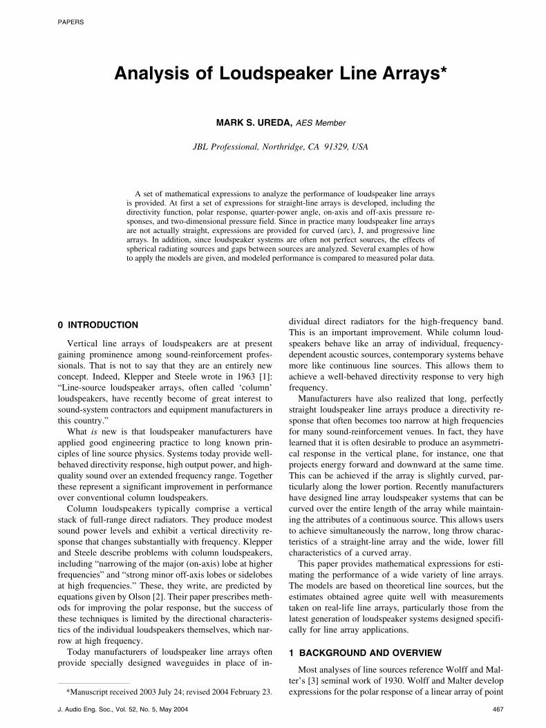
Fig. 2 shows polar response curves9 of a uniform linesource at various ratios of source length and wavelength.The polar response is wide at low ratios of L/�. As theratio is increased, the directivity pattern narrows and ex-hibits nulls and lobes. These are explored in more detail inSection 2.3.

7The time-varying factor ej�t is omitted.

8Note that the maximum pressure at any given distance andfrequency may never actually be obtained.

9A polar response curve is the directivity function expressed indecibels and plotted on a polar chart. The on-axis pressure is usedas the reference pressure, that is, polar response � 20 log [R(�)/R(0)].

Fig. 1. Geometric construction for far-field directivity function ofa line source.

PAPERS ANALYSIS OF LOUDSPEAKER LINE ARRAYS


2.3 Lobes and Nulls—UniformStraight-Line Source

Fig. 2 shows that at long wavelengths (� > L) the polarresponse of a uniform straight-line source is fairly omni-directional. At shorter wavelengths lobes and nulls areobtained. The position and magnitude of these are easilycalculated.

The far-field directivity function of a uniform linesource is given in Section 2.2 as

RU�� =sin ��L�� sin ��

��L�� sin �.

This function has the generic form of sin z/z. To evaluatethis function on axis, that is, z � 0, we must useL’Hospital’s rule, taking derivatives of the numerator anddenominator. This yields

limsin z

z→ cos �0� = 1.

The fact that the limit approaches unity indicates that therewill always be a maximum on axis. Off-axis nulls areobtained when sin z/z goes to zero. This occurs where theargument z reaches (nonzero) multiples of �. Substitutingthe full expression for z, nulls are obtained when

�L

�sin � = m�

where m is a nonzero integer. Therefore nulls are ob-tained at

�sin ��= m�

L

where m � 1, 2, 3, . . . . Off-axis lobes of the directivityfunction are found between the nulls, that is, at

�sin ��=3�

2L,5�

2L,7�

2L, . . . .

This can be written as

�sin ��=�m + 1�2��

L

where m � 1, 2, 3, . . . .Finally it is possible to calculate the amplitude of the

lobes of a uniform line source. Since the amplitude de-creases inversely with z, the pressure amplitude of the mthlobe is

Am = �cos �m��

m� + ��2�where m � 1, 2, 3, . . . .

2.4 Quarter-Power Angle—UniformStraight-Line Source

Often it is useful to determine the −6-dB angle of auniform straight-line source. This is accomplished by set-ting the generic form of the directivity function equal to0.5,10 that is,

sin z

z= 0.5.

10The directivity function is a pressure ratio. A pressure ratioof 0.5 yields a sound pressure level difference of −6 dB.

Fig. 2. Polar response curves of a uniform line source.

UREDA PAPERS


Solving numerically, z � 1.895. The −6-dB point on oneside of the central lobe is at angle �, where

z = 1.895 =�L

�sin �.

The quarter-power angle is the total included angle be-tween the −6-dB points on either side of the central lobeand is given by

�−6 dB = 2�.

Solving for � in terms of length and wavelength and sub-stituting we have

�−6 dB = 2 sin−11.895�

�L

≈ 2 sin−10.6�

L.

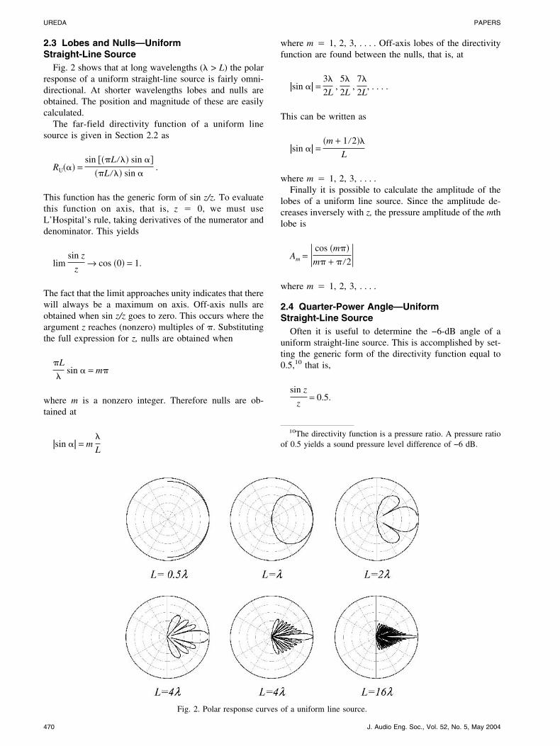
The quarter-power angle as a function of L/� is shownin Fig. 3. A similar result is obtained by Benson [19].11

At small L/�, that is, a short line source and long wave-length, the quarter-power angle is wide. At large ratios ofL/�, that is, long sources and short wavelengths, the quar-ter-power angle is narrow. For small angles,12 where sin z≈ z, the line source quarter-power angle is

�−6 dB =1.2�

L

where � is in radians. Expression � in degrees, we have

�−6 dB = 68.8�

L�degrees�.

In some cases it is convenient to use frequency ratherthan a ratio of wavelength and source length. Rewriting,the quarter-power angle equation for uniform line sourcesbecomes (approximately)

�−6 dB ≈2.4 × 104

fL

for L in meters and f in hertz, or

�−6 dB ≈7.8 × 104

fL

for L in feet and f in hertz.The directivity response of a line source is a plot of the

quarter-power angle versus frequency. The directivity re-sponse of uniform line sources of several lengths is shownin Fig. 4. These show that the quarter-power angle of largesources is quite narrow at high frequency. For instance,at 10 kHz a 4-m-long uniform straight-line source has a−6-dB angle of 0.6°.

2.5 On-Axis Pressure Response ofStraight-Line Sources

The on-axis pressure response of a line source is derivedin much the same manner as the directivity function. Thepressure radiated from each infinitely small line segmentis summed at an observation point P. In this case, how-ever, P is at a distance x along an axis normal to the sourceand no far-field assumptions are made.

2.5.1 Conventional Approach—Midpoint MethodFig. 5 shows the conventional geometric construction

used to solve for the pressure along a path normal to thesource, beginning at its midpoint. Referring to Fig. 5, L is

11Note that Benson solved for the −3-dB angle.12The small angle approximation holds for angles less than

about 30°. Note that sin (�/6) � 0.5000 and �/6 � 0.5235 sothat the error is less than 5%.

Fig. 3. Quarter-power angle of a uniform line source.Fig. 4. Directivity response of uniform line sources 1, 2, 4, and8 m long.



the total length of the source and rmid is the distance fromany radiating element dl of the source to any distance xalong the horizontal axis. The general form for the radiatedpressure at x is

pmid�x� = �−L�2

L�2 A�l� e−j�krmid�x, l�+��l��

rmid�x, l�dl

where

rmid�x, l� = �x2 + l2 .

The pressure response is the logarithmic ratio of the mag-nitude of the pressure squared at x over the magnitude ofthe pressure squared at some reference distance, that is,

R�x� = 20 log�p�x��p�xref��

.

The on-axis pressure response of a 4-m uniformstraight-line source, where A(l) = A and �(l) � 0, at 8 kHzis shown in Fig. 6. The pressure response generally de-creases at a rate of −3 dB per doubling of the distance outto approximately 100 m. It exhibits undulations in thisregion, the magnitudes of which increase as the distance

approaches 100 m. Beyond 100 m the pressure amplitudeno longer undulates and decreases monotonically at −6 dBper doubling of the distance. The point at which thischange occurs is referred to as the transition distance. Theregion between the source and the transition distance isreferred to as the near field, and the region beyond is thefar field.

The transition distance varies with source length andfrequency. Fig. 7 shows the on-axis response of three dif-ferent-length uniform line sources at 8 kHz. As the lengthL increases, the transition distance increases. Fig. 8 showsthe on-axis response of a 4-m-long uniform line source at500 Hz, 2 kHz, and 8 kHz. It illustrates that the transitiondistance also increases with frequency.

2.5.2 Midpoint versus EndpointThe conventional approach used to determine the on-

axis pressure response of a line source discussed in Sec-

Fig. 5. Geometric construction for calculating on-axis pressureresponse of a line source (midpoint convention).

Fig. 6. On-axis pressure response (from midpoint) of a uniformline source (4 m long, 8 kHz).

Fig. 7. On-axis response (from midpoint) of 2; 4; and 8-m uni-form line sources at 8 kHz. 4- and 8-meter response curves areoffset by 10 and 20 dB, respectively.

Fig. 8. On-axis response (from midpoint) of a 4-m uniform linesource at 500 Hz, 2 kHz, and 8 kHz. 2- and 8-kHz responsecurves are offset by 10 and 20 dB, respectively.

UREDA PAPERS


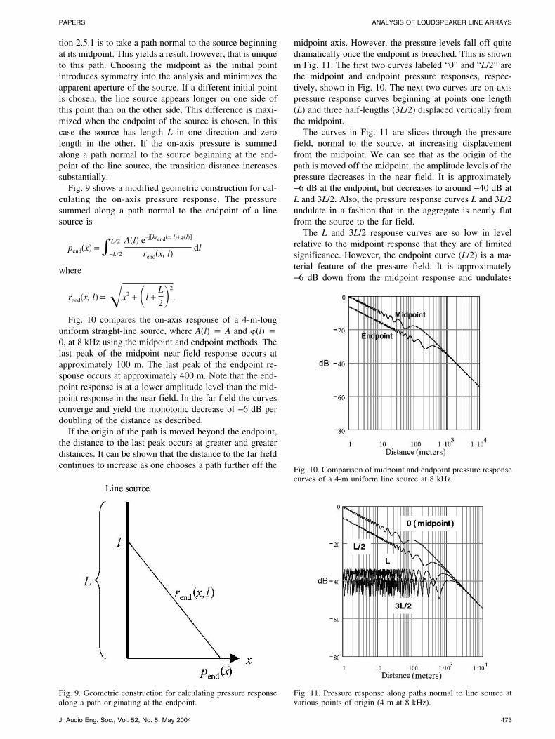
tion 2.5.1 is to take a path normal to the source beginningat its midpoint. This yields a result, however, that is uniqueto this path. Choosing the midpoint as the initial pointintroduces symmetry into the analysis and minimizes theapparent aperture of the source. If a different initial pointis chosen, the line source appears longer on one side ofthis point than on the other side. This difference is maxi-mized when the endpoint of the source is chosen. In thiscase the source has length L in one direction and zerolength in the other. If the on-axis pressure is summedalong a path normal to the source beginning at the end-point of the line source, the transition distance increasessubstantially.

Fig. 9 shows a modified geometric construction for cal-culating the on-axis pressure response. The pressuresummed along a path normal to the endpoint of a linesource is

pend�x� = �−L�2

L�2 A�l� e−j�krend�x, l�+��l��

rend�x, l�dl

where

rend�x, l� =�x2 + �l +L

2�2

.

Fig. 10 compares the on-axis response of a 4-m-longuniform straight-line source, where A(l) � A and �(l) �0, at 8 kHz using the midpoint and endpoint methods. Thelast peak of the midpoint near-field response occurs atapproximately 100 m. The last peak of the endpoint re-sponse occurs at approximately 400 m. Note that the end-point response is at a lower amplitude level than the mid-point response in the near field. In the far field the curvesconverge and yield the monotonic decrease of −6 dB perdoubling of the distance as described.

If the origin of the path is moved beyond the endpoint,the distance to the last peak occurs at greater and greaterdistances. It can be shown that the distance to the far fieldcontinues to increase as one chooses a path further off the

midpoint axis. However, the pressure levels fall off quitedramatically once the endpoint is breeched. This is shownin Fig. 11. The first two curves labeled “0” and “L/2” arethe midpoint and endpoint pressure responses, respec-tively, shown in Fig. 10. The next two curves are on-axispressure response curves beginning at points one length(L) and three half-lengths (3L/2) displaced vertically fromthe midpoint.

The curves in Fig. 11 are slices through the pressurefield, normal to the source, at increasing displacementfrom the midpoint. We can see that as the origin of thepath is moved off the midpoint, the amplitude levels of thepressure decreases in the near field. It is approximately−6 dB at the endpoint, but decreases to around −40 dB atL and 3L/2. Also, the pressure response curves L and 3L/2undulate in a fashion that in the aggregate is nearly flatfrom the source to the far field.

The L and 3L/2 response curves are so low in levelrelative to the midpoint response that they are of limitedsignificance. However, the endpoint curve (L/2) is a ma-terial feature of the pressure field. It is approximately−6 dB down from the midpoint response and undulates

Fig. 10. Comparison of midpoint and endpoint pressure responsecurves of a 4-m uniform line source at 8 kHz.

Fig. 9. Geometric construction for calculating pressure responsealong a path originating at the endpoint.

Fig. 11. Pressure response along paths normal to line source atvarious points of origin (4 m at 8 kHz).



well past the midpoint transition distance. The fact thattwo such disparate response curves can be obtained bymerely shifting the origin of the normal path demonstratesthe ambiguity of the term “on-axis response.”

2.6 Pressure Field of Straight-Line SourcesThe most comprehensive approach to observe the pres-

sure response of a line source is to compute its pressurefield. This eliminates the question of midpoint versus end-point. It is obtained by rewriting the expression for theradiated pressure in terms of Cartesian coordinates as setup in Fig. 12. The pressure at any point P is

p�x, y� = �−L�2

L�2 A�l� e−j�kr�x, y, l�+��l��

r�x, y, l�dl

where

r�x, y, l� = �x2 + �y − l�2.

Fig. 13 shows the pressure field of a 4-m uniformstraight-line source, where A(l) � A and �(l) � 0, inseveral frequency bands. The major on-axis lobe gets nar-rower with increasing frequency, as expected. The minorlobes increase in number and lower amplitude levels. Athigh frequency they dissolve into very complex patterns ofconstructive and destructive interference. Note that thepressure varies across the major lobe at 8 kHz in a mannerconsistent with the pressure slices shown in Fig. 11. Theundulations extend to a greater distance from a line normalto the endpoint than from the midpoint.

3 ARC SOURCES

Many loudspeaker line arrays used in practice are actu-ally curved. This is because pure straight-line arrays pro-duce a narrow vertical polar response at high frequency—often too narrow to reach audiences beneath and slightly infront of the array. A slightly curved array provides supe-rior coverage in this area. One important type of curvedline source is the arc source.

An arc source is comprised of radiating elements ar-ranged along a segment of a circle. At all frequencies it pro-vides a wider directivity response than a straight-line sourceof the same length. At high frequency it provides a polarpattern that corresponds to the included angle of the arc.

3.1 Polar Response of Arc SourcesThe derivation of the directivity function of an arc

source follows the same steps as described for a straight-line source. Fig. 14 shows the geometric construction of anarc source with radius R and total included angle �. Thepressure radiated by an arc at off-axis angle � is

pA�� = �−��2

��2 A�� e−j�krA��, ��+��

rA��, ��R d�.

As in Section 2.1, the evaluation of this expression issimplified if we assume that the observation point P is alarge distance away. In this case the distance is muchgreater than the length of the arc, and the distances to Pfrom any two segments along the arc are approximatelyequal. This allows us to bring the rA term in the denomi-nator to the front of the integral since by definition

1

rA��2�≈

1

rA�−��2�≈

1

rA.

Conversely, the rA term in the exponential has a signifi-cant influence on the directivity function. This is becausethe relatively small differences in distance to P from anytwo segments are not small compared to a wavelength.Fig. 14 shows that rA in the exponent can be expressed as

rA��, �� = 2R sin ��

2� sin ��

2+ ��

where � is the angle between a line that bisects the arcangle and a line from the center point of the arc to P.Substituting, the far-field directivity function of an arc isthen expressed in general form as

RA�� =��−��2

��2A�� e−j�krA��, ��+��R d�

�−��2

��2A��R d� �.

If we assume constant amplitude and zero phase shiftalong the arc, that is, A(�) � A and �(�) � 0, the direc-tivity function reduces to13

RA�� =1

R��−��2

��2e−jkrA��, ��R d��

13This integral does not have a convenient closed-form solu-tion similar to the one obtained for the line array. Wolff andMalter [3] provide a point source summation version of the di-rectivity function as follows:

R�� =1

2m + 1�n=−m

n=m

cos�2�R

�cos �� + n��

+ in=−m

n=m

sin�2�R

�cos �� + n��

where m is an integer, 2m + 1 is the number of point sources, and� is the angle subtended between any two adjacent point courses.

Fig. 12. Geometric construction for pressure field of a linesource.

UREDA PAPERS


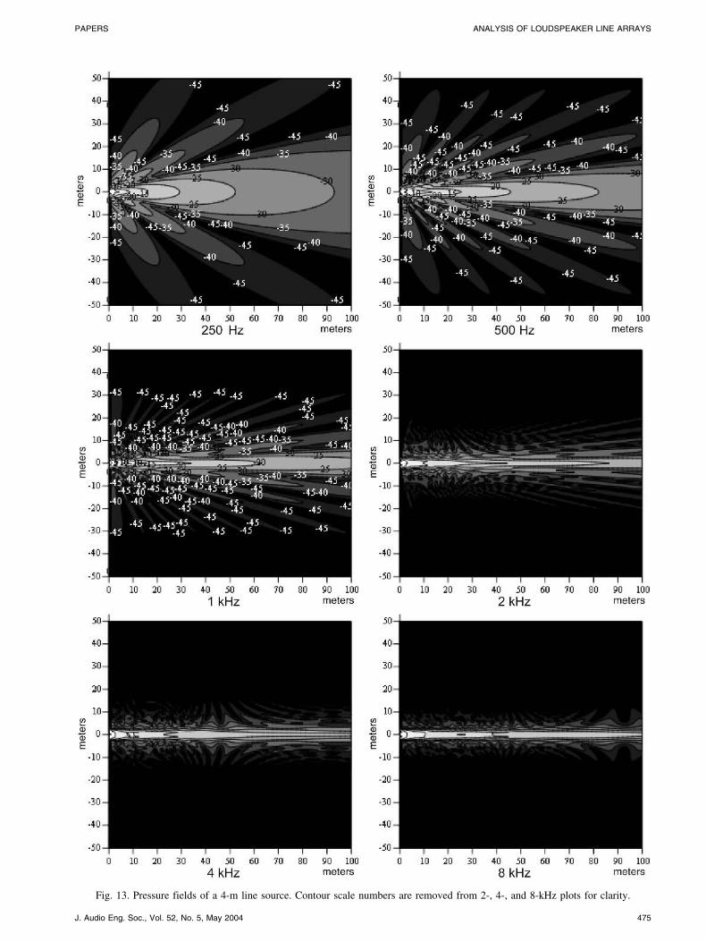
Fig. 13. Pressure fields of a 4-m line source. Contour scale numbers are removed from 2-, 4-, and 8-kHz plots for clarity.



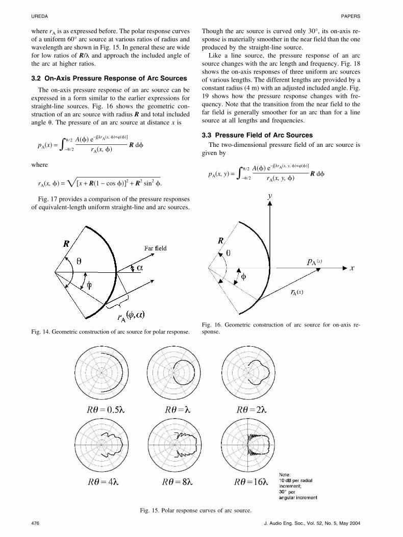
where rA is as expressed before. The polar response curvesof a uniform 60° arc source at various ratios of radius andwavelength are shown in Fig. 15. In general these are widefor low ratios of R/� and approach the included angle ofthe arc at higher ratios.

3.2 On-Axis Pressure Response of Arc Sources

The on-axis pressure response of an arc source can beexpressed in a form similar to the earlier expressions forstraight-line sources. Fig. 16 shows the geometric con-struction of an arc source with radius R and total includedangle �. The pressure of an arc source at distance x is

pA�x� = �−��2

��2 A�� e−j�krA�x, ��+��

rA�x, ��R d�

where

rA�x, �� = ��x + R�1 − cos ��2 + R2 sin2 �.

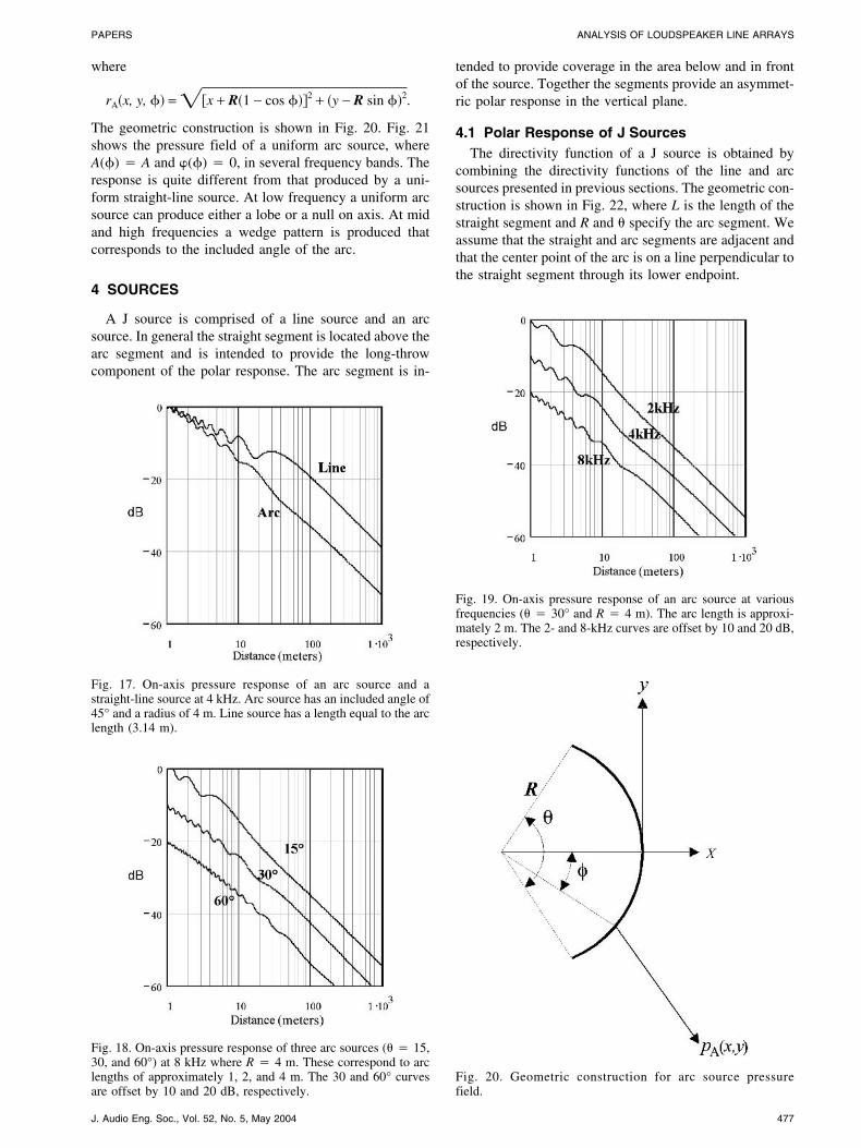
Fig. 17 provides a comparison of the pressure responsesof equivalent-length uniform straight-line and arc sources.

Though the arc source is curved only 30°, its on-axis re-sponse is materially smoother in the near field than the oneproduced by the straight-line source.

Like a line source, the pressure response of an arcsource changes with the arc length and frequency. Fig. 18shows the on-axis responses of three uniform arc sourcesof various lengths. The different lengths are provided by aconstant radius (4 m) with an adjusted included angle. Fig.19 shows how the pressure response changes with fre-quency. Note that the transition from the near field to thefar field is generally smoother for an arc than for a linesource at all lengths and frequencies.

3.3 Pressure Field of Arc SourcesThe two-dimensional pressure field of an arc source is

given by

pA�x, y� = �−��2

��2 A�� e−j�krA�x, y, ��+��

rA�x, y, ��R d�

Fig. 14. Geometric construction of arc source for polar response.

Fig. 15. Polar response curves of arc source.

Fig. 16. Geometric construction of arc source for on-axis re-sponse.

UREDA PAPERS


where

rA�x, y, �� = ��x + R�1 − cos ��2 + �y − R sin ��2.

The geometric construction is shown in Fig. 20. Fig. 21shows the pressure field of a uniform arc source, whereA(�) � A and �(�) � 0, in several frequency bands. Theresponse is quite different from that produced by a uni-form straight-line source. At low frequency a uniform arcsource can produce either a lobe or a null on axis. At midand high frequencies a wedge pattern is produced thatcorresponds to the included angle of the arc.

4 SOURCES

A J source is comprised of a line source and an arcsource. In general the straight segment is located above thearc segment and is intended to provide the long-throwcomponent of the polar response. The arc segment is in-

tended to provide coverage in the area below and in frontof the source. Together the segments provide an asymmet-ric polar response in the vertical plane.

4.1 Polar Response of J SourcesThe directivity function of a J source is obtained by

combining the directivity functions of the line and arcsources presented in previous sections. The geometric con-struction is shown in Fig. 22, where L is the length of thestraight segment and R and � specify the arc segment. Weassume that the straight and arc segments are adjacent andthat the center point of the arc is on a line perpendicular tothe straight segment through its lower endpoint.

Fig. 17. On-axis pressure response of an arc source and astraight-line source at 4 kHz. Arc source has an included angle of45° and a radius of 4 m. Line source has a length equal to the arclength (3.14 m).

Fig. 18. On-axis pressure response of three arc sources (� � 15,30, and 60°) at 8 kHz where R � 4 m. These correspond to arclengths of approximately 1, 2, and 4 m. The 30 and 60° curvesare offset by 10 and 20 dB, respectively.

Fig. 19. On-axis pressure response of an arc source at variousfrequencies (� � 30° and R � 4 m). The arc length is approxi-mately 2 m. The 2- and 8-kHz curves are offset by 10 and 20 dB,respectively.

Fig. 20. Geometric construction for arc source pressurefield.



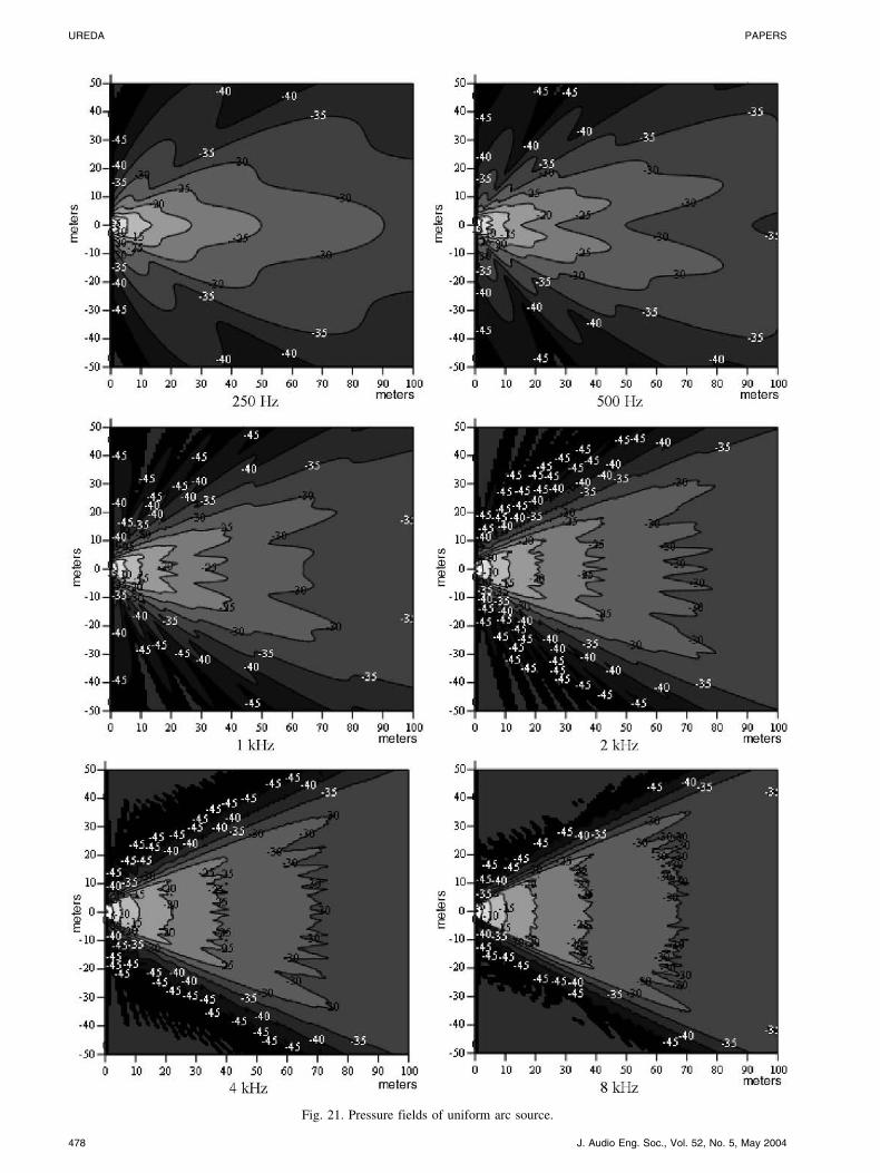
Fig. 21. Pressure fields of uniform arc source.

UREDA PAPERS


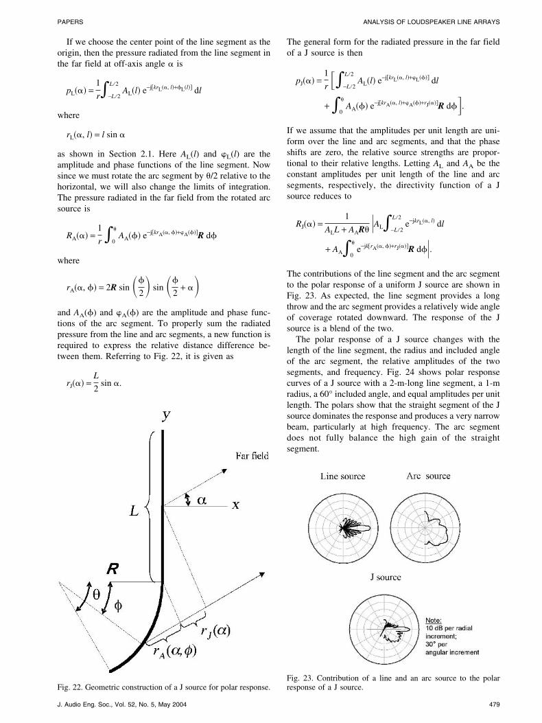
If we choose the center point of the line segment as theorigin, then the pressure radiated from the line segment inthe far field at off-axis angle � is

pL�� =1

r�−L�2

L�2AL�l� e−j�krL��, l�+�L�l�� dl

where

rL��, l� = l sin �

as shown in Section 2.1. Here AL(l) and �L(l) are theamplitude and phase functions of the line segment. Nowsince we must rotate the arc segment by �/2 relative to thehorizontal, we will also change the limits of integration.The pressure radiated in the far field from the rotated arcsource is

RA�� =1

r �0

�

AA�� e−j�krA��, ��+�A��R d�

where

rA��, �� = 2R sin ��

2� sin ��

2+ ��

and AA(�) and �A(�) are the amplitude and phase func-tions of the arc segment. To properly sum the radiatedpressure from the line and arc segments, a new function isrequired to express the relative distance difference be-tween them. Referring to Fig. 22, it is given as

rJ�� =L

2sin �.

The general form for the radiated pressure in the far fieldof a J source is then

pJ�� =1

r ��−L�2

L�2AL�l� e−j�krL��, l�+�L�� dl

+ �0

�

AA�� e−j�krA��, l�+�A��+rJ��R d��.

If we assume that the amplitudes per unit length are uni-form over the line and arc segments, and that the phaseshifts are zero, the relative source strengths are propor-tional to their relative lengths. Letting AL and AA be theconstant amplitudes per unit length of the line and arcsegments, respectively, the directivity function of a Jsource reduces to

RJ�� =1

ALL + AAR��AL�−L�2

L�2e−jkrL��, l� dl

+ AA�0

�

e−jk�rA��, ��+rJ��R d��.The contributions of the line segment and the arc segmentto the polar response of a uniform J source are shown inFig. 23. As expected, the line segment provides a longthrow and the arc segment provides a relatively wide angleof coverage rotated downward. The response of the Jsource is a blend of the two.

The polar response of a J source changes with thelength of the line segment, the radius and included angleof the arc segment, the relative amplitudes of the twosegments, and frequency. Fig. 24 shows polar responsecurves of a J source with a 2-m-long line segment, a 1-mradius, a 60° included angle, and equal amplitudes per unitlength. The polars show that the straight segment of the Jsource dominates the response and produces a very narrowbeam, particularly at high frequency. The arc segmentdoes not fully balance the high gain of the straightsegment.

Fig. 22. Geometric construction of a J source for polar response.Fig. 23. Contribution of a line and an arc source to the polarresponse of a J source.



There are several approaches to providing a more bal-anced response. One is to make the straight segmentshorter, thereby reducing the gain. A second is to increaseAA relative to AL. For instance, one might use a J sourcethat has a 1-m-long straight segment (as opposed to 2 m inthe previous example) and set AA � 2AL (instead of AA �AL). The polar response of this modified J source is con-siderably more balanced than the uniform J source, asshown in Fig. 25.

4.2 On-Axis Pressure Response ofJ Sources

The on-axis pressure response of a J source is obtainedby combining the pressure response functions of the lineand arc sources presented in the preceding. The geometricconstruction is shown in Fig. 26, where L is the length ofthe straight segment, and R and � specify the arc segment.Note that the lower endpoint of the arc segment is taken asthe initial point for the on-axis response. Based on thisgeometry, the pressure radiated at point P from a Jsource is

pJ�x� = �0

L AL�l� e−j�krL�x, l�+�L�l��

rL�x, l�dl

+ �0

� AA�� e−j�krA�x, ��+�A��

rA�x, ��R d�

where

rL�x, l� = �x2 + �R sin � + l�2

rA�x, �� = ��x + R�1 − cos ��2 + R2�sin � − sin ��2.

Fig. 27 compares the on-axis pressure responses of uni-form equivalent-length straight-line and J sources, whereA(�) � A. The straight segment of the J source dominatesthe response, producing undulations in the near field verysimilar to those of the straight-line source. However, theon-axis aperture of the J source is foreshortened relative tothe equal-length line source, so the distance to the far fieldis marginally shorter.

4.3 Pressure Field of J Sources

The geometric construction for the pressure field of a Jsource is shown in Fig. 28. The general form for the pres-sure at P is

pJ�x, y� = �0

L AL�l� e−j�krL�x, y, l�+�L��

rL�x, y, l�dl

+ R�0

� AA�� e−j�krA�x, y, ��+�A��

rA�x, y, ��d�

Fig. 24. J-source polar response curves (Example 1). L � 2 m, R � 1 m, � � 60°, AL � 1, AA � 1.

UREDA PAPERS


where

rL�x, y, l� = �x2 + �y + l�2

rA�x, y, �� = ��x + R�1 − cos ��2 + �y + L + R sin ��2.

The pressure field of a uniform J source, where A(�) � Aand �(�) � 0 in several frequency bands, is shown inFig. 29. The parameters of the J source are the same asthose used for the modified J source described in Section

4.1, that is, a 1-m straight segment and AA � 2AL. Theseplots show clearly that a J source is a blend of straight andarc sources. This is particularly true at mid and high frequen-cies, where the constituent responses are easily identifiable.

5 PROGRESSIVE SOURCES

Like a J source, a progressive source provides an asym-metric polar response in the vertical plane. However,

Fig. 25. J-source polar response curves (Example 2). L � 1 m, R � 1 m, � � 60°, AL � 1, AA � 2.

Fig. 26. Geometric construction of a J source for on-axis pressureresponse.

Fig. 27. Comparison at 2 kHz of on-axis pressure response of a4-m-long straight-line source and a J source. L � 2 m, R � 2 m,� � 60°, AL � 1, AA � 1.



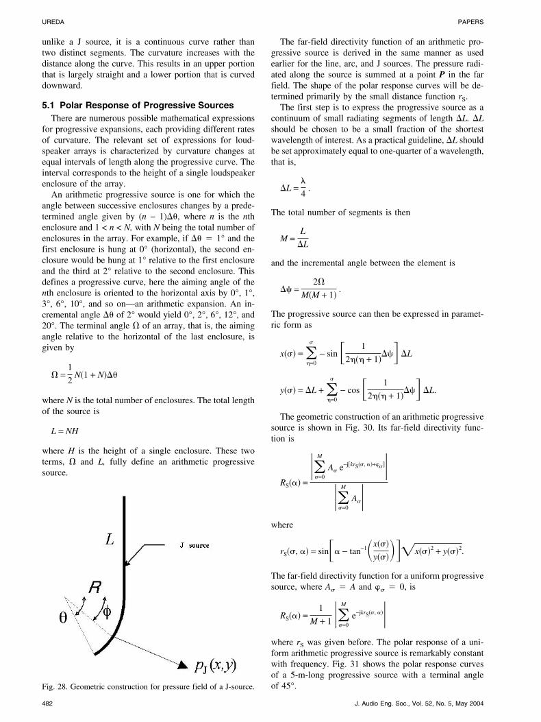
unlike a J source, it is a continuous curve rather thantwo distinct segments. The curvature increases with thedistance along the curve. This results in an upper portionthat is largely straight and a lower portion that is curveddownward.

5.1 Polar Response of Progressive SourcesThere are numerous possible mathematical expressions

for progressive expansions, each providing different ratesof curvature. The relevant set of expressions for loud-speaker arrays is characterized by curvature changes atequal intervals of length along the progressive curve. Theinterval corresponds to the height of a single loudspeakerenclosure of the array.

An arithmetic progressive source is one for which theangle between successive enclosures changes by a prede-termined angle given by (n − 1)��, where n is the nthenclosure and 1 < n < N, with N being the total number ofenclosures in the array. For example, if �� 1° and thefirst enclosure is hung at 0° (horizontal), the second en-closure would be hung at 1° relative to the first enclosureand the third at 2° relative to the second enclosure. Thisdefines a progressive curve, here the aiming angle of thenth enclosure is oriented to the horizontal axis by 0°, 1°,3°, 6°, 10°, and so on—an arithmetic expansion. An in-cremental angle �� of 2° would yield 0°, 2°, 6°, 12°, and20°. The terminal angle of an array, that is, the aimingangle relative to the horizontal of the last enclosure, isgiven by

=1

2N�1 + N��

where N is the total number of enclosures. The total lengthof the source is

L = NH

where H is the height of a single enclosure. These twoterms, and L, fully define an arithmetic progressivesource.

The far-field directivity function of an arithmetic pro-gressive source is derived in the same manner as usedearlier for the line, arc, and J sources. The pressure radi-ated along the source is summed at a point P in the farfield. The shape of the polar response curves will be de-termined primarily by the small distance function rS.

The first step is to express the progressive source as acontinuum of small radiating segments of length �L. �Lshould be chosen to be a small fraction of the shortestwavelength of interest. As a practical guideline, �L shouldbe set approximately equal to one-quarter of a wavelength,that is,

�L =�

4.

The total number of segments is then

M =L

�L

and the incremental angle between the element is

� =2

M�M + 1�.

The progressive source can then be expressed in paramet-ric form as

x�� = �=0

�

− sin � 1

2�� + 1�� L

y�� = �L + �=0

�

− cos � 1

2�� + 1�� L.

The geometric construction of an arithmetic progressivesource is shown in Fig. 30. Its far-field directivity func-tion is

RS�� =�

�=0

M

A� e−j�krS��, ��+��

�=0

M

A��where

rS��, �� = sin�� − tan−1�x��

y��x��2 + y��2.

The far-field directivity function for a uniform progressivesource, where A� � A and �� 0, is

RS�� =1

M + 1��=0

M

e−jkrS��, ��where rS was given before. The polar response of a uni-form arithmetic progressive source is remarkably constantwith frequency. Fig. 31 shows the polar response curvesof a 5-m-long progressive source with a terminal angleof 45°.Fig. 28. Geometric construction for pressure field of a J-source.

UREDA PAPERS


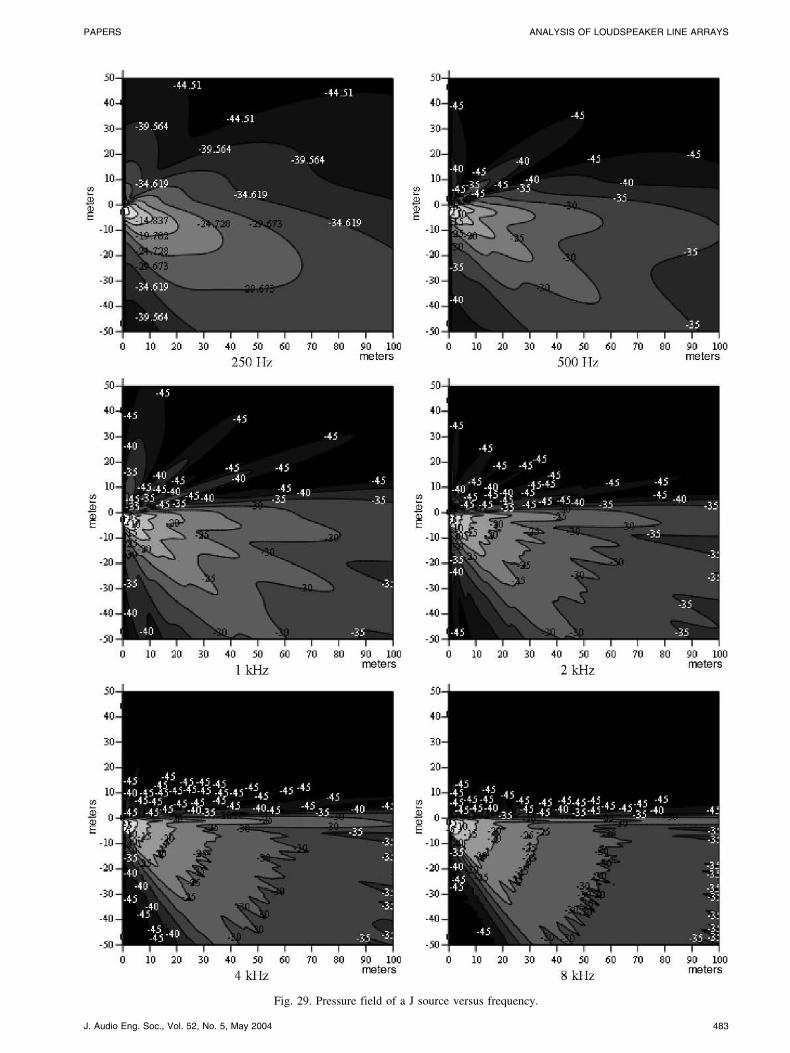
Fig. 29. Pressure field of a J source versus frequency.



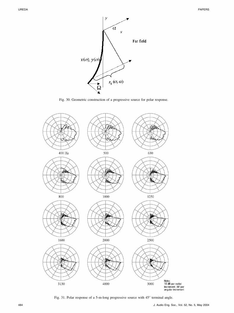
Fig. 30. Geometric construction of a progressive source for polar response.

Fig. 31. Polar response of a 5-m-long progressive source with 45° terminal angle.

UREDA PAPERS


5.2 On-Axis Pressure Response ofProgressive Sources

The geometric construction for the on-axis pressure re-sponse of a progressive source is shown in Fig. 32. Thepressure response along a path from the lower end is

pS�x� = �=0

M

A�

e−j�krS�x, ��+ ��

rS�x, ��

where

rS�x, �� = ��x − x��2 + �y�M� − y��2

and A� is the amplitude at element � and �� is the relativephase at element �.

Fig. 33 compares the on-axis response curves of equiva-lent-length uniform straight-line and progressive sources.These curves show that the progressive source has reducedundulations in the near field and a smoother transitionfrom the near field to the far field.

5.3 Pressure Field of Progressive SourcesThe geometric construction for the pressure field of a

progressive source is shown in Fig. 34. The pressure at anypoint P is

pS�x, y� = �=0

M

A�

e−j�krS�x, y, ��+ ��

rS�x, y, ��

where

rS�x, y, �� = ��x − x��2 + �y − y��2.

The pressure field of a uniform progressive source in sev-eral frequency bands is shown in Fig. 35. These resultsillustrate the well-behaved asymmetrical response of aprogressive source that makes them an excellent geometryupon which to base loudspeaker arrays for sound-reinforcement applications.

6 ADVANCED TOPICS

As a practical matter, large line arrays of loudspeakersare not perfectly continuous line sources. For instance,they may have gaps between the loudspeaker enclosuresbecause of enclosure construction material or spacing.These gaps are effectively nonradiating portions of the lineand may have an effect on the performance of the array.Also, certain radiating elements in loudspeaker line arraysmay produce radial wavefronts instead of pure, flat wave-fronts. This may also have an effect on the performance ofthe array. These topics are analyzed in the following sections.

6.1 Gaps in Line SourcesIn previous sections we assume that each type of line

source is continuous along its entire length. In practice,

Fig. 32. Geometric construction of a progressive source for on-axis pressure response.

Fig. 33. Pressure response comparison at 2 kHz of a 45° terminalangle, 4-m-long progressive source and a line source of the samelength.

Fig. 34. Geometric construction for pressure field of a progressive source.



Fig. 35. Pressure fields of a progressive source versus frequency.

UREDA PAPERS


however, it may not be possible to achieve this. For in-stance, the thickness of the material used to construct aloudspeaker enclosure does not radiate acoustic energy.When loudspeaker enclosures are stacked into an array,these nonradiating segments are distributed along thelength of the array. This can be modeled by limiting theintegration of the line source to the radiating portions only.Referring to Fig. 36, d is the dimension of the nonradiatingelement on either side of the radiating element.

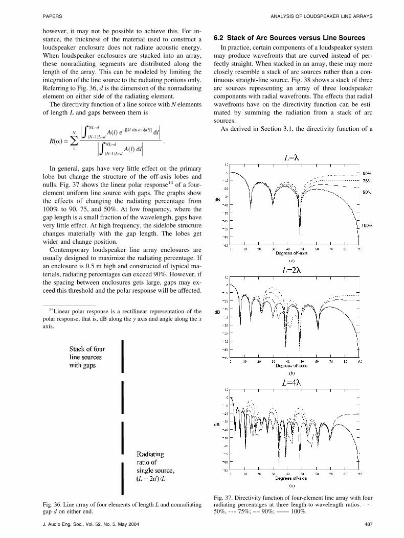
The directivity function of a line source with N elementsof length L and gaps between them is

R�� = 1

N ��N−1�L+d

NL−dA�l� e−j�kl sin �+��l�� dl�

��N−1�L+d

NL−dA�l� dl� .

In general, gaps have very little effect on the primarylobe but change the structure of the off-axis lobes andnulls. Fig. 37 shows the linear polar response14 of a four-element uniform line source with gaps. The graphs showthe effects of changing the radiating percentage from100% to 90, 75, and 50%. At low frequency, where thegap length is a small fraction of the wavelength, gaps havevery little effect. At high frequency, the sidelobe structurechanges materially with the gap length. The lobes getwider and change position.

Contemporary loudspeaker line array enclosures areusually designed to maximize the radiating percentage. Ifan enclosure is 0.5 m high and constructed of typical ma-terials, radiating percentages can exceed 90%. However, ifthe spacing between enclosures gets large, gaps may ex-ceed this threshold and the polar response will be affected.

6.2 Stack of Arc Sources versus Line SourcesIn practice, certain components of a loudspeaker system

may produce wavefronts that are curved instead of per-fectly straight. When stacked in an array, these may moreclosely resemble a stack of arc sources rather than a con-tinuous straight-line source. Fig. 38 shows a stack of threearc sources representing an array of three loudspeakercomponents with radial wavefronts. The effects that radialwavefronts have on the directivity function can be esti-mated by summing the radiation from a stack of arcsources.

As derived in Section 3.1, the directivity function of a

14Linear polar response is a rectilinear representation of thepolar response, that is, dB along the y axis and angle along the xaxis.

Fig. 36. Line array of four elements of length L and nonradiatinggap d on either end.

Fig. 37. Directivity function of four-element line array with fourradiating percentages at three length-to-wavelength ratios. - � -50%, - - - 75%; –– 90%; —— 100%.



uniform arc source is

RA�� =1

R��−��2

��2e−jkrA��, ��R d��

where

rA��, �� = 2R sin ��

2� sin ��

2+ ��.

Here R is the radius and � the included angle of the arc.The directivity function of a stack of arc sources is ob-tained by applying the first product theorem.15 In this casethe directivity function of the arc is multiplied by thedirectivity function of an array of simple sources. Thefar-field directivity function for an array of N simplesources of equal amplitude and phase distributed a dis-tance D apart along a line is given by

RP�� =1

N�n=1

N

e−j�k�n−1�D sin ��.Applying the first product theorem, the directivity func-

tion of a vertical stack of arc sources is

RAP�� = RA��RP��.

Fig. 39 shows the effects of nonflat wavefronts on thedirectivity function of the sources, compared to a perfectlyflat wavefront. As with gaps in a line source, a curvatureprimarily produces changes in the lobe/null structure of

the off-axis response. The changes increase with increas-ing curvature and are more predominant when the curva-ture is a material fraction of a wavelength.

Fig. 39(a) compares the directivity function of a uni-form line source of length 3L with an array of three curvedsources of length L, where the curvature � of the arc isone-eighth wavelength. The directivity functions are verysimilar, with only small differences in the lobe/null struc-

15The first product theorem states that the directional factor ofan array of identical sources is the product of the directionalfactor of the array and the directional factor of a single elementof the array. See Kinsler et al. [20].

Fig. 38. Stack of three arc sources of radius R, included angle �,and curvature �.

Fig. 39. Comparison of directivity functions of a stack of threecurved sources and a straight-line source. Curved sources haveelement length L � 150 mm, total included angle � � 20°.Straight-line source has total length 3L.

UREDA PAPERS


ture. In particular, note that the nulls at approximately 18,35, and 60° are not as deep with the stack of arcsources.

Fig. 39(b) and (c) shows the directivity functions of theuniform line and the three-element array at curvatures ofone-quarter and one-half wavelengths. In these cases,lobes gradually replace the nulls at 18, 35, and 60°. Atone-quarter wavelength the lobe at 18° is approximately10 dB below the level of the on-axis lobe, up from ap-proximately 20 dB. This represents a practical limit to thecurvature, which maintains, generally speaking, the direc-tivity function of a pure line source. The response at one-half wavelength is unacceptable as the 18° lobe is herenearly equal in amplitude to the primary lobe.

This one-quarter-wavelength limit on curvature allowsus to estimate, for a given curvature, the practical upperfrequency limit for which it maintains the directivity re-sponse of a uniform line source. If a source has an element

length L of 130 mm and a total arc angle of 20°, then

� =L

2tan��

4� = 6.6 mm

and the upper frequency limit is

f =c

4�≈ 13 kHz.

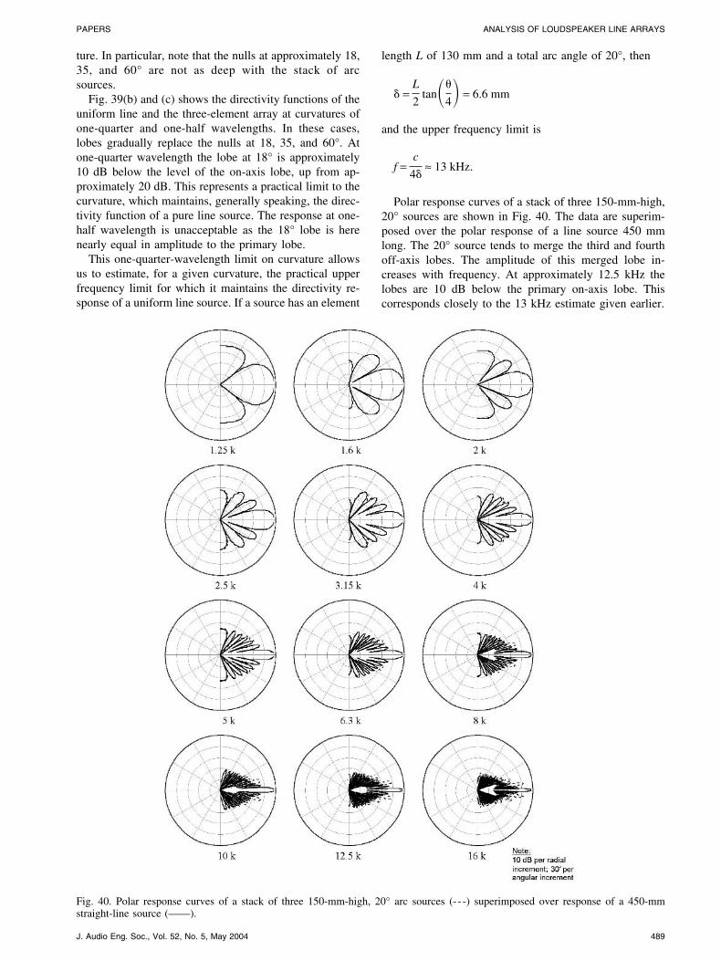
Polar response curves of a stack of three 150-mm-high,20° sources are shown in Fig. 40. The data are superim-posed over the polar response of a line source 450 mmlong. The 20° source tends to merge the third and fourthoff-axis lobes. The amplitude of this merged lobe in-creases with frequency. At approximately 12.5 kHz thelobes are 10 dB below the primary on-axis lobe. Thiscorresponds closely to the 13 kHz estimate given earlier.

Fig. 40. Polar response curves of a stack of three 150-mm-high, 20° arc sources (- - -) superimposed over response of a 450-mmstraight-line source (——).



7 APPLICATIONS

The mathematical models developed in the previoussections will provide useful estimates of the performanceof many types of loudspeaker line arrays. However, theaccuracy of the estimates may be compromised by severalfactors. First, real-life loudspeaker systems do not oftenbehave like perfect sources. In addition to the gaps andradial wavefronts discussed in Section 6, other potentialfactors include cone or diaphragm breakup, suspensionand magnetic nonlinearities, and enclosure resonance andedge (diffraction) effects. Second, collecting far-field datacan be problematic since the microphone must be placed atlarge distances. Most anechoic chambers provide adequate

distances to measure only relatively small arrays. Largearrays can be measured outdoors, but environmental fac-tors such as wind and atmospheric turbulence may affectresults. Alternatively, data may be taken in a large indoorspace, but the acoustical characteristics of the room mustbe isolated and removed from the measurements. None-theless, despite all of these potential sources of errors,useful estimates can be produced, as illustrated in the fol-lowing examples.

7.1 Example 1: Small Straight-LineArray—Low-Frequency Model

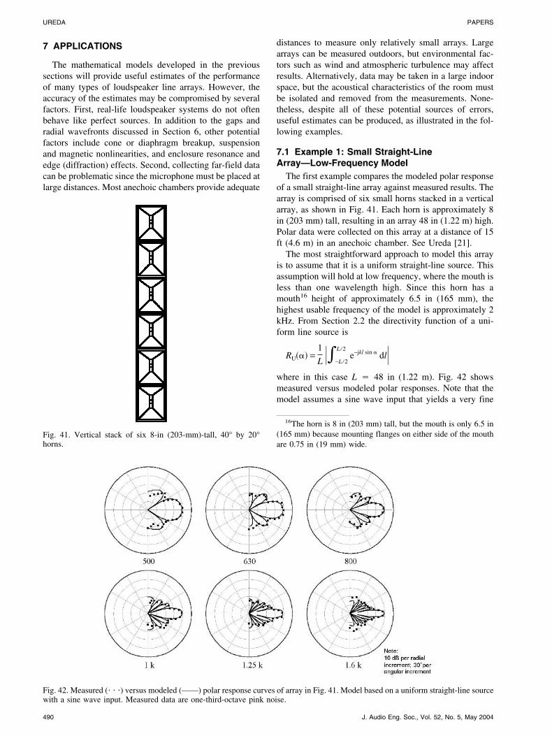
The first example compares the modeled polar responseof a small straight-line array against measured results. Thearray is comprised of six small horns stacked in a verticalarray, as shown in Fig. 41. Each horn is approximately 8in (203 mm) tall, resulting in an array 48 in (1.22 m) high.Polar data were collected on this array at a distance of 15ft (4.6 m) in an anechoic chamber. See Ureda [21].

The most straightforward approach to model this arrayis to assume that it is a uniform straight-line source. Thisassumption will hold at low frequency, where the mouth isless than one wavelength high. Since this horn has amouth16 height of approximately 6.5 in (165 mm), thehighest usable frequency of the model is approximately 2kHz. From Section 2.2 the directivity function of a uni-form line source is

RU�� =1

L ��−L�2

L�2e−jkl sin � dl�

where in this case L � 48 in (1.22 m). Fig. 42 showsmeasured versus modeled polar responses. Note that themodel assumes a sine wave input that yields a very fine

16The horn is 8 in (203 mm) tall, but the mouth is only 6.5 in(165 mm) because mounting flanges on either side of the mouthare 0.75 in (19 mm) wide.

Fig. 41. Vertical stack of six 8-in (203-mm)-tall, 40° by 20°horns.

Fig. 42. Measured (� � �) versus modeled (——) polar response curves of array in Fig. 41. Model based on a uniform straight-line sourcewith a sine wave input. Measured data are one-third-octave pink noise.

UREDA PAPERS


lobe and null structure. The measured data are one-third-octave pink noise, which tends to fill the sharp nulls of asine wave response. Nonetheless, the modeled responseclosely resembles the measured data. Note that the 1.5-in(38-mm) gaps between the horn mouths do not materiallyaffect the modeled performance.

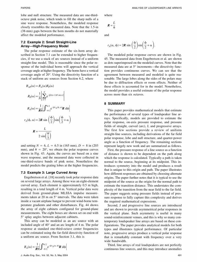
7.2 Example 2: Small Straight-LineArray—High-Frequency Model

The polar response estimate of the six-horn array de-scribed in Section 7.1 can be extended to higher frequen-cies, if we use a stack of arc sources instead of a uniformstraight-line model. This is reasonable since the polar re-sponse of the individual horns will approach the verticalcoverage angle at higher frequency. The horns have a verticalcoverage angle of 20°. Using the directivity function of astack of uniform arc sources from Section 6.2, where

RAP�� = RA��RP��

RP�� =1

N�n=1

N

e−j�k�n−1�D sin ��RA�� =

1

R��−��2

��2e−jkrA��, ��R d��

rA��, �� = 2R sin ��

2�sin��

2+ ��

R =L

2 sin��

2�and setting N � 6, L � 6.5 in (165 mm), D � 8 in (203mm), and � � 20°, we obtain the polar response curvesshown in Fig. 43. Again, the curves are based on a sinewave response, and the measured data were collected inone-third-octave bands of pink noise. Nonetheless themodel predicts the grating lobes at the higher frequencies.

7.3 Example 3: Large Curved ArrayEngebretson et al. [18] recently took polar response data

on several large arrays. Among these was an eight-elementcurved array. Each element is approximately 0.5 m high,resulting in a total length of 4 m. Vertical polar data werederived from ground-plane MLSSA impulse measure-ments taken at 20 m on 5° intervals. The data were takeninside a vacant airplane hangar to prevent wind-borne tem-perature gradients and other disturbances. Fig. 44 showsthe array of eight cabinets configured for ground-planemeasurements. The eight boxes are shown set on end with5° splay angles between adjacent cabinets.

This array can be modeled as an arc source with anincluded angle of 40° and an arc length of 4 m. The polarresponse at standard one-third-octave center frequenciescan be estimated using the far-field directivity function ofa uniform arc source. From Section 3.1, this is

RA�� =1

R��−��2

��2e−jkrA��, ��R d��

where

R =L

�

and

rA��, �� = 2R sin ��

2�sin��

2+ ��.

The modeled polar response curves are shown in Fig.45. The measured data from Engebretson et al. are shownas dots superimposed on the modeled curves. Note that themeasured data are at 5° increments—the directivity func-tion provides continuous curves. We can see that theagreement between measured and modeled is quite rea-sonable. The large lobes along the sides of the polars maybe due to diffraction effects or room effects. Neither ofthese effects is accounted for in the model. Nonetheless,the model provides a useful estimate of the polar responseacross more than six octaves.

8 SUMMARY

This paper provides mathematical models that estimatethe performance of several types of loudspeaker line ar-rays. Specifically, models are provided to estimate thepolar response, on-axis pressure response, and pressurefields of straight, curved (arc), J, and progressive arrays.The first few sections provide a review of uniformstraight-line sources, including derivations of the far fieldpolar response, lobe and null structure, and quarter-powerangle as a function of frequency. The remaining sectionsrepresent largely new work and are summarized as follows.

First, the pressure response of a line source as a functionof distance is shown to be dependent on the path alongwhich the response is calculated. Typically a path is takennormal to the source, beginning at its midpoint. This in-troduces symmetry into the model and produces a resultthat is unique to this origin and path. The paper illustrateshow different responses are obtained by choosing alternateorigins. The paper further notes that it is typical to use themidpoint of the source as the origin for the normal path toestimate the transition distance. This understates the com-plexity of the transition from the near field to the far field.The paper suggests using pressure fields instead of pres-sure response to fully capture this complexity and derivesthe required mathematical expressions.

Second, J and progressive line sources are introducedand are shown to provide asymmetrical polar responses inthe vertical plane. Such asymmetry is useful in manysound-reinforcement venues, and this is why so many con-temporary loudspeaker line arrays are based on these con-figurations. The paper provides analytical models for bothtypes and illustrates typical performance. Of particularnote, progressive arrays produce a vertical polar responsethat is remarkably constant with frequency over a verywide bandwidth.

Third, line arrays of real loudspeakers are not perfectlycontinuous line sources, and this may introduce anomalies



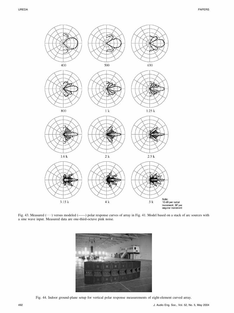
Fig. 43. Measured (� � �) versus modeled (——) polar response curves of array in Fig. 41. Model based on a stack of arc sources witha sine wave input. Measured data are one-third-octave pink noise.

Fig. 44. Indoor ground-plane setup for vertical polar response measurements of eight-element curved array.

UREDA PAPERS


into their response. The paper provides a model that showsthe effect of gaps in line sources that are introduced by thethickness of the loudspeaker enclosure construction mate-rial. The model shows that at low frequency, where thegap length is a small fraction of the wavelength, gaps havevery little effect. At high frequency the sidelobe structurechanges materially with the gap length. The lobes getwider and change position. As a practical matter, contem-

porary loudspeaker line array enclosures are usually de-signed to maximize the radiating percentage, often in ex-cess of 90%. This minimizes the effects of gaps across theuseful bandwidth.

Fourth, real loudspeaker elements may not produce per-fectly flat wavefronts, so that a vertical stack of loudspeak-ers does not provide a perfectly straight-line source. Thepaper provides an analytical model to estimate the effect

Fig. 45. Measured polar response data (� � �) shown against predicted polar response of eight-element curved array.



of the curvature of the elemental sources of a line array. Itshows that the effects are frequency dependent and negli-gible as long as the curvature is less than one-quarterwavelength.

Finally, measured polar response data of two differentloudspeaker line arrays were compared to modeled results.In general the models produce very good estimates ofactual performance despite the fact that loudspeaker non-linearities, enclosure diffraction, and environmental ef-fects among others are not accounted for. Robust resultscan be obtained for a wide variety of array types across anextended frequency range of interest.

ACKNOWLEDGMENT

The author would like to express his appreciation to hiscolleagues at JBL Professional, including Mark Gander,David Scheirman, Mark Engebretson, and Doug Button.They piqued his interest in line arrays, encouraged andsupported this body of work, and were always fun to workwith.

10 REFERENCES

[1] D. L. Klepper and D. W. Steele, “Constant Direc-tional Characteristics from a Line Source Array,” AudioEng. Soc., vol. 11, no. 3, p. 198 (1963).

[2] H. F. Olson, Elements of Acoustical Engineering,1st ed. (Van Nostrand, New York, 1940), p. 25.

[3] I. Wolff and L. Malter, “Directional Radiation ofSound, J. Acoust. Soc. Am., vol. 2, no. 2, p. 201 (1930).

[4] L. Beranek, Acoustics, 1st ed. (McGraw-Hill, NewYork, 1954).

[5] A. B. Wood, A Textbook of Sound (Bell and Sons,London, 1957).

[6] A. H. Davis, Modern Acoustics, 1st ed. (Macmillan,New York, 1934), p. 63.

[7] M. Rossi, Acoustics and Electroacoustics (ArtechHouse, Norwood, MA, 1988).

[8] E. Skudrzyk, The Foundations of Acoustics(Springer, New York, 1971).

[9] S. P. Lipshitz and J. Vanderkooy, “The AcousticRadiation of Line Sources of Finite Length,” presented atthe 81st Convention of the Audio Engineering Society, J.

Audio Eng. Soc. (Abstracts), vol. 34, pp. 1032–1033 (1986Dec.), preprint 2417.

[10] D. L. Smith, “Discrete-Element Line Arrays—Their Modeling and Optimization,” J. Audio Eng. Soc.,vol. 45, pp. 948–964 (1997 Nov.).

[11] J. Eargle, Handbook of Sound System Design(ELAR Publ., Commack, NY, 1989).

[12] C. Heil, “Sound Fields Radiated by MultipleSound Source Arrays,” presented at the 92nd Conventionof the Audio Engineering Society, J. Audio Eng. Soc. (Ab-stracts), vol. 40, p. 440 (1992 May), preprint 3269.

[13] M. Junger and D. Feit, Sound, Structures, andTheir Interactions (MIT Press, Cambridge, MA, 1972).

[14] M. S. Ureda, “Line Arrays: Theory and Applica-tions,” presented at the 110th Convention of the AudioEngineering Society, J. Audio Eng. Soc. (Abstracts), vol.49, p. 526 (2001 June), convention paper 5304.

[15] M. S. Ureda, “J and Spiral Line Arrays,” presentedat the 111th Convention of the Audio Engineering Society,J. Audio Eng. Soc. (Abstracts), vol. 49, p. 1233 (2001Dec.), convention paper 5485.

[16] M. S. Urban, C. Heil, and P. Bauman, “WavefrontSculpture Technology,” J. Audio Eng. Soc. (EngineeringReports), vol. 51, pp. 912–932 (2003 Oct.).

[17] D. Button, “High-Frequency Components forHigh-Output Articulated Line Arrays,” presented at the113th Convention of the Audio Engineering Society, J.Audio Eng. Soc. (Abstracts), vol. 50, p. 957 (2002 Nov.),convention paper 5650.

[18] M. E. Engebretson, M. S. Ureda, and D. J. Button,“Directional Radiation Characteristics of Articulating LineArray Loudspeaker Systems,” presented at the 111th Con-vention of the Audio Engineering Society, J. Audio Eng.Soc. (Abstracts), vol. 49, p. 1233 (2001 Dec.).

[19] J. E. Benson, “Theory and Applications of Elec-trically Tapered Electro-Acoustic Arrays,” in IREE Int.Electronics Conv. Digest (1975 Aug.), pp. 587–589.

[20] L. Kinsler, A. Frey, A. Coppens, and J. Sanders,Fundamentals of Acoustics, 4th ed. (Wiley, New York,1982).

[21] M. S. Ureda, “Wave Field Synthesis with HornArrays,” presented at the 100th Convention of the AudioEngineering Society, J. Audio Eng. Soc. (Abstracts), vol.44, p. 630 (1996 July/Aug.), preprint 4144.

THE AUTHOR

UREDA PAPERS


Mark Ureda received a B.S. degree in engineering fromUCLA, an M.S. degree in acoustics from Penn State, and anM.B.A. from the UCLA Graduate School of Management.

Mr. Ureda joined the Altec Lansing Corporation in1976 as an engineer in the acoustics research group. Therehe codeveloped the Mantaray constant directivity horns. In1980 he was promoted to director of acoustics and led thedevelopment of several new lines of horns and loudspeak-ers. He left the company when it was sold in 1984 andbegan a career in aerospace. He returned to audio in 1990as a consultant to Mark IV Audio, where he developed

ArraySHOW, a software package that computes radiatedsound fields of horn arrays. In 1999 he joined JBL Pro-fessional and developed the VerTec line array calculator.Audio is a hobby for him. He continues his aerospacecareer at Northrop Grumman, where he is the corporatevice president of Strategy and Technology. He is respon-sible for strategy development and mergers and acquisi-tions in the space and electronics segments.

Mr. Ureda has authored numerous technical papers onhorns, directivity measurements, line sources, and loud-speaker/horn arrays.



Documents

Analysis of Loudspeaker Line Arrays*...performance of loudspeaker line arrays. Section 7 com-pares the modeled and measured polar response curves of three loudspeaker line arrays