Analysis of Demersal Fish Assemblages in Selected ...pubs.iclarm.net/resource_centre/AMF_Chapter-11-FA.pdf · Analysis of Demersal Fish Assemblages in Selected Philippine Fishing

227

Analysis of Demersal Fish Assemblages in Selected Philippine Fishing Grounds

Wilfredo L. CamposDivision of Biological Sciences

College of Arts & SciencesUniversity of the Philippines in the Visayas

Miag-ao, Iloilo, 5023 Philippines

Campos, W.L. 2003. Analysis of demersal fish assemblages in selected Philippine fishing grounds, p. 227 - 248. In G. Silvestre, L. Garces, I. Stobutzki, M. Ahmed, R.A. Valmonte-Santos, C. Luna, L. Lachica-Aliño, P. Munro, V. Christensen and D. Pauly (eds.) Assessment, Management and Future Directions for Coastal Fisheries in Asian Countries. WorldFish Center Conference Proceedings 67, 1 120 p.

Abstract

This paper presents the results of analyses of demersal fish assemblages in various fishing grounds in the Philippines. Data from exploratory trawl surveys conducted in 1947 - 49 show that the 24 fishing grounds covered by the survey can be arranged along a gradient of substrate type (i.e. relative coral cover and sediment characteristics). These may be used to determine the species commonly caught in these grounds. A trend of increasing catch rates with decreasing water depth and increasing proportion of mud in the substrate was noted. Data from more recent systematic surveys in Samar Sea (1979 - 80), San Pedro Bay (1994 - 95) and Manila Bay (1992 - 93) were analyzed to examine spatio-temporal patterns in fish assem-blages. In all 3 areas, the fish community was characterized by a large number of ubiquitous species, with Leiognathids comprising at least 28% of the total catch. In terms of habitat relations, depth was the primary factor in Samar Sea and San Pedro Bay, where transitions in fish assemblage composition were recognizable at certain depth ranges. In Manila Bay, however, species composition appears to be more related to location (inner versus outer portions of the bay).

Analysis of data from five locations (Manila Bay, Tayabas Bay, Sorsogon Bay, Samar Sea and San Pedro Bay) extending from the western to the eastern portions of the country showed similar seasonality, with fish assemblage composition varying slightly during the monsoon season.

Introduction

This paper summarizes analyses of data from se-lected trawl surveys conducted in the Philippines. The trawl data sources include (1) exploratory sur-veys (1947 - 49) in 24 fishing grounds around the country; (2) systematic trawl surveys in Samar Sea (1979 - 80), San Pedro Bay (1994 - 95) and Manila Bay (1992 - 93); and (3) quasi-systematic surveys for demersal biomass in Tayabas Bay (1994 - 95) and Sorsogon Bay (1994 - 95). Data were analyzed

to: identify assemblages of trawl-caught organisms; examine how these are distributed in space and time within the surveyed areas; and determine if the different areas surveyed showed similar patterns. This information, in turn, can help in the delineation of assemblage boundaries and fishing zones appli-cable to various fishing grounds in the country.

Historical (1947 - 49) data were analyzed to exam-ine the broad pattern of demersal fish assemblages in the country prior to the expansion of the trawl

228 WorldFish Center 229

fishery in the mid-1970s. This provides insight into possible changes in the composition of demersal resources since that period, and whether such changes are indicative of ecosystem overfishing as reported in other heavily-fished areas.

Materials and Methods

The initial task of the study was to determine the distribution of demersal assemblages in space and time. Because the surveys had different objectives, there are differences in content and resolution of their information. For example, the exploratory surveys did very limited sampling in each fishing ground. The quasi-systematic surveys consisted of monthly sampling, but because fixed trawl stations were not used, this precluded spatial distribution analyses. Only the systematic surveys (with fixed sampling time intervals and trawl stations) allowed analyses across space and time. It was therefore not possible to employ a standard set of analyses for all the surveys. The general approach in data analyses is described in this section, while analytic details are given in separate sections dealing with the dif-ferent data sets.

Data from the exploratory surveys were used to characterize the 24 fishing grounds with respect to species group composition and apparent habitat characteristics. Data from the systematic and quasi-systematic surveys were then analyzed to examine potential temporal patterns, and to see if similar patterns occur in different areas of the country. Lastly, data from the systematic trawl surveys were examined for extensive spatial analyses and for comparison between seasons.

Temporal Distribution

The objective here was to determine if any of the areas examined showed seasonality in species com-position of the catch (e.g. seasonal differences in species caught in an area or relative abundance of the species). To do this, seasons or time slices (i.e. month groupings) within a year were determined by clustering months based on monthly species abundances (i.e. all stations combined). The result-ing seasons then served as the time slices within which spatial distributions were further examined.

Spatial Distribution

The spatial distribution of demersal assemblages

was examined at 2 levels: at the annual or within year level, and at the seasonal level. An annual characterization of species assemblages and habi-tats within each survey area was done by combin-ing all monthly species abundance data for each station and then performing the cluster analysis. At the seasonal level, species abundance data for months in the time slice were combined for each station. The stations were then clustered to show the distribution of habitats within the area.

Internal AnalysisCluster Analysis

All cluster analyses were executed using Two-Way INdicator SPecies ANalysis (TWINSPAN) (Hill, 1979), which produced two-way tables in which the row (species) arrangement corresponds to the species clusters (species assemblages) and the col-umn (sample = station or month) arrangement cor-responds to the sample clusters (i.e. stations form habitats, months form seasons). Dendrograms were constructed using the information contained in the output files of the software. These provide a visual presentation of the similarity or dissimilarity bet-ween the formed clusters. Ordinations were con-ducted as a way to verify the clusters formed (see below). Where necessary, a frequency of occur-rence of 5 - 10% was used as criteria to limit the number of species included in the analysis. Because of apparent reading errors in the software, all data were first transformed (natural logarithms) and pseudospecies cut levels were then determined from a frequency table of the transformed data.

Ordination Analysis

Ordination of samples (stations or months) in “spe-cies space” and “sample space” was performed using Detrended Correspondence Analysis (DCA) in the CANOCO program (Ter Braak 1988). Ordination is a method of plotting samples on a coordinate system representing gradients in species abundance (species space) or plotting species along axes repre-senting station (i.e. habitat) or month (i.e. season) preferences (sample space). These plots reveal how distinct (or indistinct) the TWINSPAN-generated clusters were from each other, or how effective the clustering method was.

External Analysis

External analysis refers to the technique of relating community data to habitat information that is


normally not included, and thus external to, the typical samples-by-species data matrix. For the systematic and quasi-systematic trawl surveys, only depth could be extracted (when not recorded) as the habitat factor available for the various stations. It was only with the exploratory surveys that any useful habitat (fishing ground) informa-tion other than depth could be extracted, and thus sensibly subjected to external analyses.

Exploratory Trawl Surveys (1947 - 49)

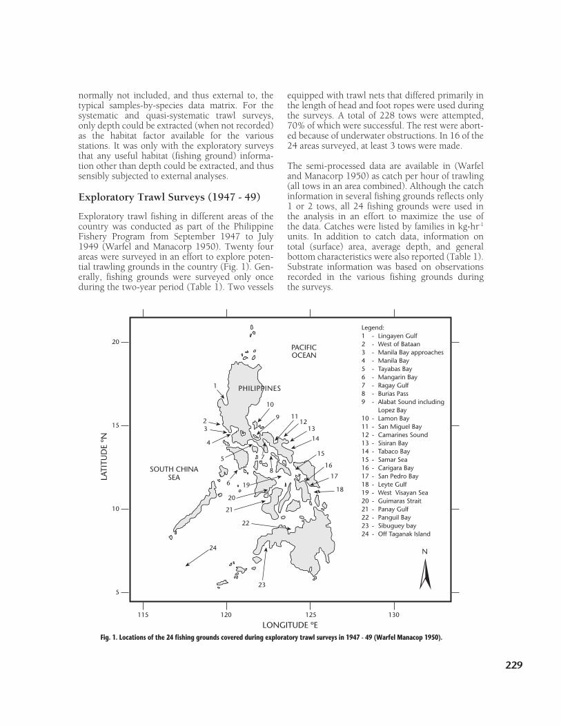
Exploratory trawl fishing in different areas of the country was conducted as part of the Philippine Fishery Program from September 1947 to July 1949 (Warfel and Manacorp 1950). Twenty four areas were surveyed in an effort to explore poten-tial trawling grounds in the country (Fig. 1). Gen-erally, fishing grounds were surveyed only once during the two-year period (Table 1). Two vessels

equipped with trawl nets that differed primarily in the length of head and foot ropes were used during the surveys. A total of 228 tows were attempted, 70% of which were successful. The rest were abort-ed because of underwater obstructions. In 16 of the 24 areas surveyed, at least 3 tows were made.

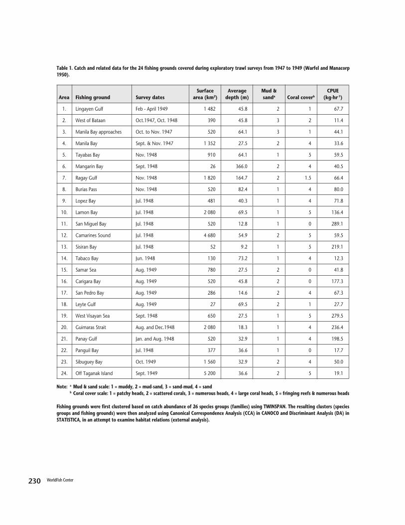
The semi-processed data are available in (Warfel and Manacorp 1950) as catch per hour of trawling (all tows in an area combined). Although the catch information in several fishing grounds reflects only 1 or 2 tows, all 24 fishing grounds were used in the analysis in an effort to maximize the use of the data. Catches were listed by families in kg.hr-1 units. In addition to catch data, information on total (surface) area, average depth, and general bottom characteristics were also reported (Table 1). Substrate information was based on observations recorded in the various fishing grounds during the surveys.

Fig. 1. Locations of the 24 fishing grounds covered during exploratory trawl surveys in 1947 - 49 (Warfel Manacop 1950).

1

10

9 1112

13

14

15

16

17

18

23

4

5

6 19

20

21

22

23

7

8

24

LATI

TUD

E ºN

115 120 125 130

20

15

10

5

LONGITUDE ºE

Legend:1 - Lingayen Gulf2 - West of Bataan3 - Manila Bay approaches4 - Manila Bay5 - Tayabas Bay6 - Mangarin Bay7 - Ragay Gulf8 - Burias Pass9 - Alabat Sound including Lopez Bay10 - Lamon Bay11 - San Miguel Bay12 - Camarines Sound13 - Sisiran Bay14 - Tabaco Bay15 - Samar Sea16 - Carigara Bay17 - San Pedro Bay18 - Leyte Gulf19 - West Visayan Sea20 - Guimaras Strait21 - Panay Gulf22 - Panguil Bay23 - Sibuguey bay24 - Off Taganak Island

N

PHILIPPINES

SOUTH CHINASEA

PACIFICOCEAN


Area Fishing ground Survey datesSurface

area (km2)Average

depth (m)Mud & sanda Coral coverb

CPUE(kg·hr-1)

1. Lingayen Gulf Feb - April 1949 1 482 45.8 2 1 67.7

2. West of Bataan Oct.1947, Oct. 1948 390 45.8 3 2 11.4

3. Manila Bay approaches Oct. to Nov. 1947 520 64.1 3 1 44.1

4. Manila Bay Sept. & Nov. 1947 1 352 27.5 2 4 33.6

5. Tayabas Bay Nov. 1948 910 64.1 1 5 59.5

6. Mangarin Bay Sept. 1948 26 366.0 2 4 40.5

7. Ragay Gulf Nov. 1948 1 820 164.7 2 1.5 66.4

8. Burias Pass Nov. 1948 520 82.4 1 4 80.0

9. Lopez Bay Jul. 1948 481 40.3 1 4 71.8

10. Lamon Bay Jul. 1948 2 080 69.5 1 5 136.4

11. San Miguel Bay Jul. 1948 520 12.8 1 0 289.1

12. Camarines Sound Jul. 1948 4 680 54.9 2 5 59.5

13. Sisiran Bay Jul. 1948 52 9.2 1 5 219.1

14. Tabaco Bay Jun. 1948 130 73.2 1 4 12.3

15. Samar Sea Aug. 1949 780 27.5 2 0 41.8

16. Carigara Bay Aug. 1949 520 45.8 2 0 177.3

17. San Pedro Bay Aug. 1949 286 14.6 2 4 67.3

18. Leyte Gulf Aug. 1949 27 69.5 2 1 27.7

19. West Visayan Sea Sept. 1948 650 27.5 1 5 279.5

20. Guimaras Strait Aug. and Dec.1948 2 080 18.3 1 4 236.4

21. Panay Gulf Jan. and Aug. 1948 520 32.9 1 4 198.5

22. Panguil Bay Jul. 1948 377 36.6 1 0 17.7

23. Sibuguey Bay Oct. 1949 1 560 32.9 2 4 50.0

24. Off Taganak Island Sept. 1949 5 200 36.6 2 5 19.1

Table 1. Catch and related data for the 24 fishing grounds covered during exploratory trawl surveys from 1947 to 1949 (Warfel and Manacorp 1950).

Note: a Mud & sand scale: 1 = muddy, 2 = mud-sand, 3 = sand-mud, 4 = sand b Coral cover scale: 1 = patchy heads, 2 = scattered corals, 3 = numerous heads, 4 = large coral heads, 5 = fringing reefs & numerous heads Fishing grounds were first clustered based on catch abundance of 26 species groups (families) using TWINSPAN. The resulting clusters (species groups and fishing grounds) were then analyzed using Canonical Correspondence Analysis (CCA) in CANOCO and Discriminant Analysis (DA) in STATISTICA, in an attempt to examine habitat relations (external analysis).


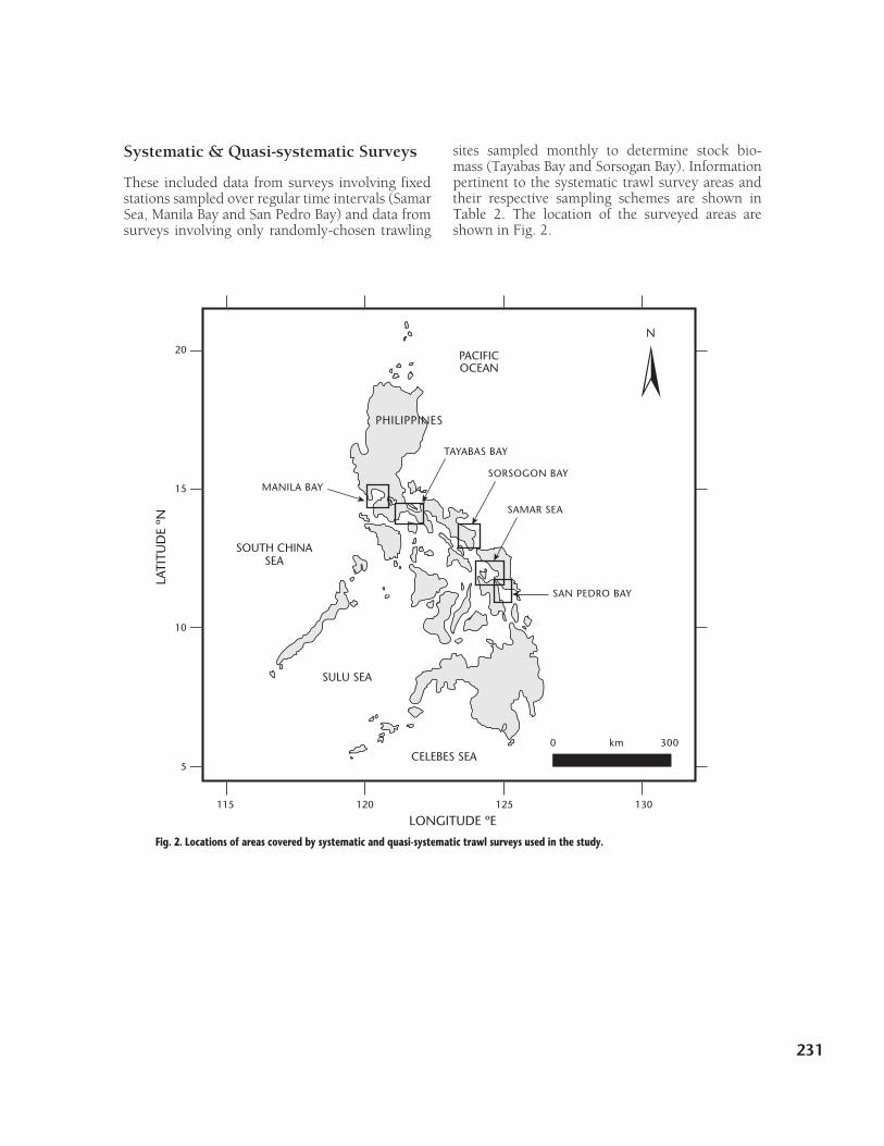
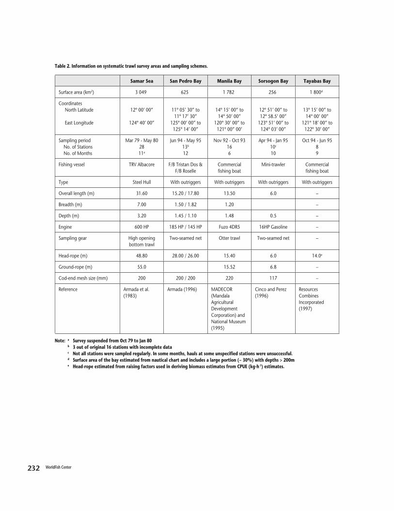
Systematic & Quasi-systematic Surveys

These included data from surveys involving fixed stations sampled over regular time intervals (Samar Sea, Manila Bay and San Pedro Bay) and data from surveys involving only randomly-chosen trawling

sites sampled monthly to determine stock bio-mass (Tayabas Bay and Sorsogan Bay). Information pertinent to the systematic trawl survey areas and their respective sampling schemes are shown in Table 2. The location of the surveyed areas are shown in Fig. 2.

Fig. 2. Locations of areas covered by systematic and quasi-systematic trawl surveys used in the study.

LATI

TUD

E ºN

115 120 125 130

20

15

10

5

LONGITUDE ºE

N

PHILIPPINES

SOUTH CHINASEA

PACIFICOCEAN

TAYABAS BAY

SORSOGON BAY

SAMAR SEA

SAN PEDRO BAY

MANILA BAY

CELEBES SEA

SULU SEA

0 km 300


Table 2. Information on systematic trawl survey areas and sampling schemes.

Samar Sea San Pedro Bay Manila Bay Sorsogon Bay Tayabas Bay

Surface area (km2) 3 049 625 1 782 256 1 800d

Coordinates North Latitude

East Longitude

12º 00’ 00”

124º 40’ 00”

11º 05’ 30” to11º 17’ 30”

125º 00’ 00” to125º 14’ 00”

14º 15’ 00” to14º 50’ 00”

120º 30’ 00” to121º 00” 00’

12º 51’ 00” to12º 58.5’ 00”

123º 51’ 00” to124º 03’ 00”

13º 15’ 00” to14º 00’ 00”

121º 18’ 00” to122º 30’ 00”

Sampling period No. of Stations No. of Months

Mar 79 - May 802811a

Jun 94 - May 9513b

12

Nov 92 - Oct 93166

Apr 94 - Jan 9510c

10

Oct 94 - Jun 9589

Fishing vessel TRV Albacore F/B Tristan Dos & F/B Roselle

Commercial fishing boat

Mini-trawler Commercial fishing boat

Type Steel Hull With outriggers With outriggers With outriggers With outriggers

Overall length (m) 31.60 15.20 / 17.80 13.50 6.0 –

Breadth (m) 7.00 1.50 / 1.82 1.20 –

Depth (m) 3.20 1.45 / 1.10 1.48 0.5 –

Engine 600 HP 185 HP / 145 HP Fuzo 4DR5 16HP Gasoline –

Sampling gear High opening bottom trawl

Two-seamed net Otter trawl Two-seamed net –

Head-rope (m) 48.80 28.00 / 26.00 15.40 6.0 14.0e

Ground-rope (m) 55.0 15.52 6.8 –

Cod-end mesh size (mm) 200 200 / 200 220 117 –

Reference Armada et al. (1983)

Armada (1996) MADECOR (Mandala Agricultural Development Corporation) and National Museum (1995)

Cinco and Perez (1996)

Resources Combines Incorporated (1997)

Note: a Survey suspended from Oct 79 to Jan 80 b 3 out of original 16 stations with incomplete data c Not all stations were sampled regularly. In some months, hauls at some unspecified stations were unsuccessful. d Surface area of the bay estimated from nautical chart and includes a large portion (~ 30%) with depths > 200m e Head-rope estimated from raising factors used in deriving biomass estimates from CPUE (kg·h-1) estimates.


For the systematic trawl surveys, both spatial and temporal distributions of species and samples were analyzed. For samples, station clusters reflect (spatial) habitats, while month clusters (temporal-annual) reflect seasons of the species clusters (spe-cies assemblages) formed. To examine seasonality in the distribution of species and habitats (tempo-ral-seasonal), spatial analyses were also conducted within each time slice formed in the temporal annual analyses.

In the case of quasi-systematic surveys, only tempo-ral analyses could be done, since sampling stations were randomly chosen in each sampling period. This allowed a comparison of seasons (i.e. formed by month clusters based on temporal species oc-currences and abundances) among different areas of the country.

Results Exploratory Trawl Survey (1947 - 49)

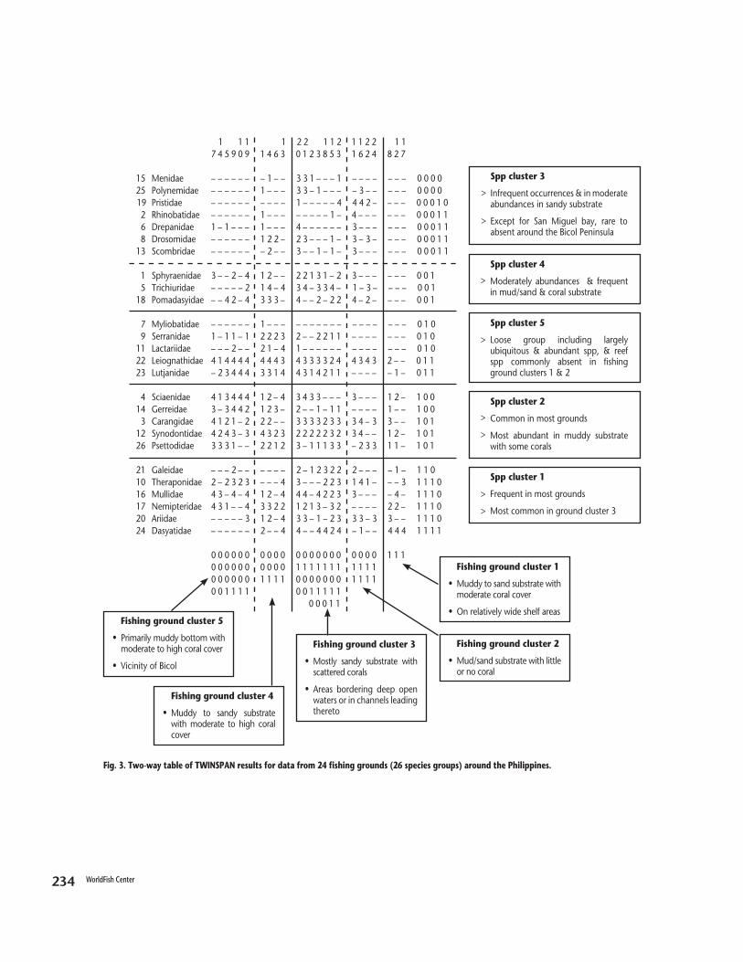
The two-way table formed by the resulting clusters of families and fishing grounds is shown in Fig. 3. The families formed 2 broad groups. One is un-common or even absent in (the first 2 groups of) fishing grounds, where the substrate is a mixture of mud and sand, with low to moderate coral cover. The other broad group is relatively common in these grounds, and includes typical soft-bottom demersal families, such as Sciaenidae, Gerreidae,

Synodontidae, Psettodidae and Nemipteridae. Spe-cies clusters 4 and 5 were most frequently recorded in fishing grounds with sandy substrate and coral cover ranging from low to high. These include com-mon reef groups such as Sphyraenidae, Pomadasy-idae, Serranidae and Lutjanidae.

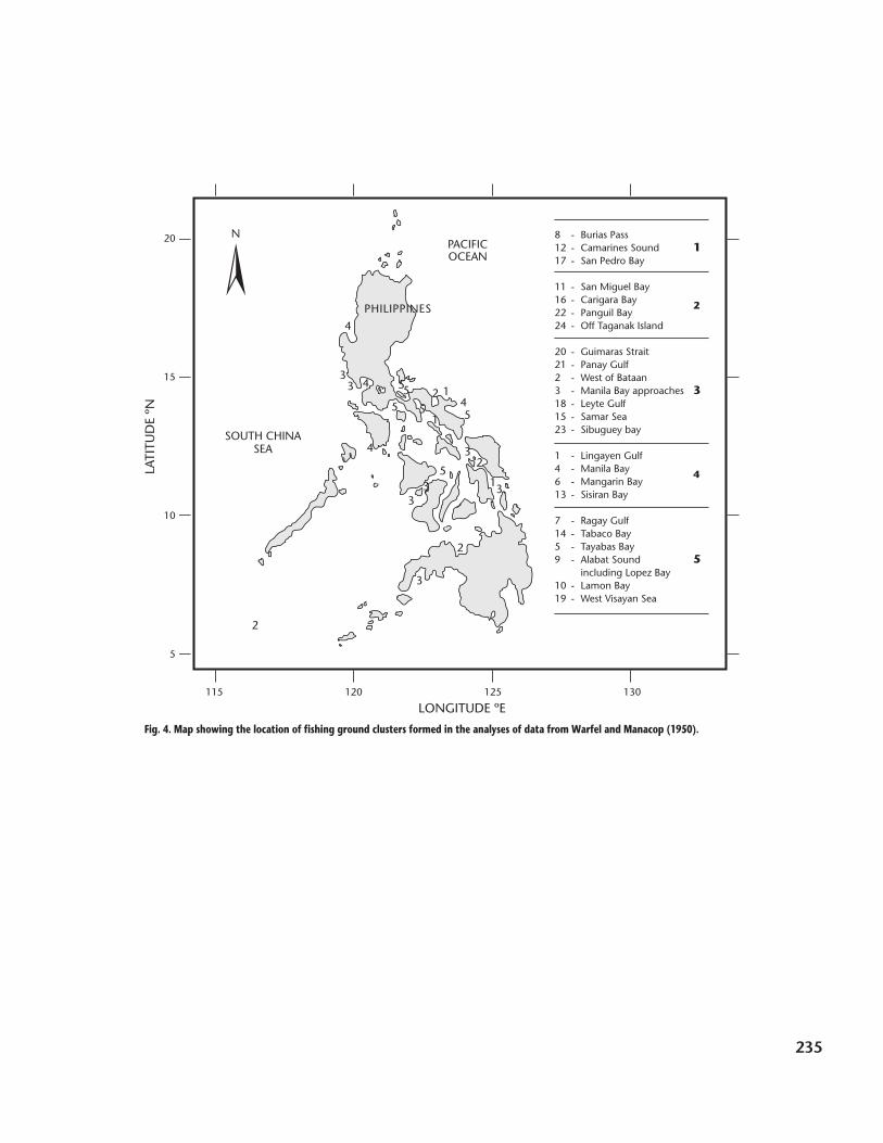
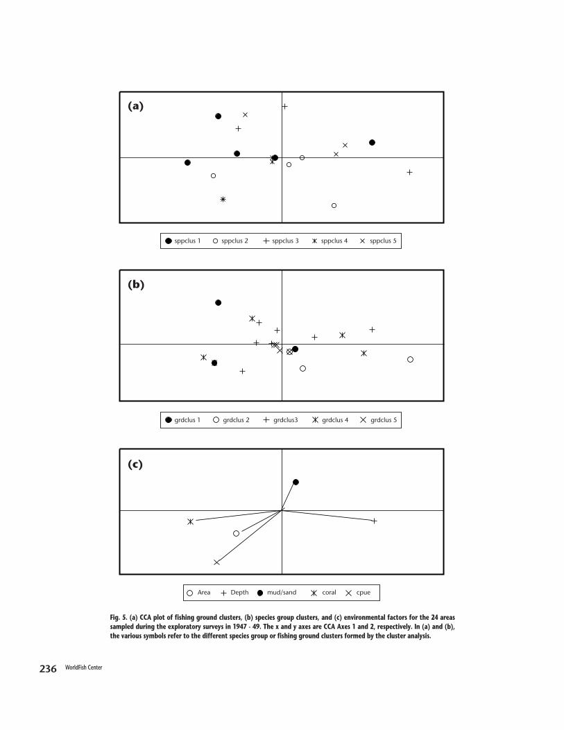
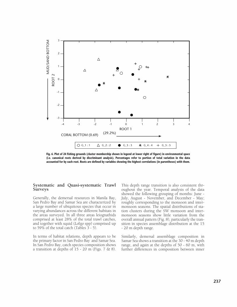
Figure 4 shows the clustering of fishing grounds superimposed on a map of the country. Figs. 5a and b show the CCA plots of the fishing ground and species group clusters formed by the cluster analyses, while Fig. 5c shows the plot of environ-mental factors in the same ordination space. Figure 6 shows the 24 areas in environmental space, based on canonical roots resulting from discriminant analysis. The results of the latter, while not allowing direct correlations with habitat factors, are never-theless consistent with those suggested by the clus-ters and by the CCA. It thus appears that the 24 areas can be arranged in gradients reflecting their substrate make-up (i.e. relative coral cover and sediment characteristics), which in turn somewhat determines the kind of species commonly caught in them. These characteristics however do not dis-count the importance of other factors such as water depth. Catch rate (kg·hr-1) was negatively correlated with both average water depth (-0.48, p < 0.05) and mud/sand substrate (-0.51, p < 0.05), and reflects an underlying trend of increasing catch rates in areas with shallower and more muddy bot-toms. This is also consistent with the distribution of the more abundant families in the catches (e.g. Leiognathidae, Mullidae).


Fig. 3. Two-way table of TWINSPAN results for data from 24 fishing grounds (26 species groups) around the Philippines.

1 1 1 1 2 2 1 1 2 1 1 2 2 1 1 7 4 5 9 0 9 1 4 6 3 0 1 2 3 8 5 3 1 6 2 4 8 2 7 15 Menidae – – – – – – – 1 – – 3 3 1 – – – 1 – – – – – – – 0 0 0 0 25 Polynemidae – – – – – – 1 – – – 3 3 – 1 – – – – 3 – – – – – 0 0 0 0 19 Pristidae – – – – – – – – – – 1 – – – – – 4 4 4 2 – – – – 0 0 0 1 0 2 Rhinobatidae – – – – – – 1 – – – – – – – – 1 – 4 – – – – – – 0 0 0 1 1 6 Drepanidae 1 – 1 – – – 1 – – – 4 – – – – – – 3 – – – – – – 0 0 0 1 1 8 Drosomidae – – – – – – 1 2 2 – 2 3 – – – 1 – 3 – 3 – – – – 0 0 0 1 1 13 Scombridae – – – – – – – 2 – – 3 – – 1 – 1 – 3 – – – – – – 0 0 0 1 1 1 Sphyraenidae 3 – – 2 – 4 1 2 – – 2 2 1 3 1 – 2 3 – – – – – – 0 0 1 5 Trichiuridae – – – – – 2 1 4 – 4 3 4 – 3 3 4 – 1 – 3 – – – – 0 0 1 18 Pomadasyidae – – 4 2 – 4 3 3 3 – 4 – – 2 – 2 2 4 – 2 – – – – 0 0 1 7 Myliobatidae – – – – – – 1 – – – – – – – – – – – – – – – – – 0 1 0 9 Serranidae 1 – 1 1 – 1 2 2 2 3 2 – – 2 2 1 1 – – – – – – – 0 1 0 11 Lactariidae – – – 2 – – 2 1 – 4 1 – – – – – – – – – – – – – 0 1 0 22 Leiognathidae 4 1 4 4 4 4 4 4 4 3 4 3 3 3 3 2 4 4 3 4 3 2 – – 0 1 1 23 Lutjanidae – 2 3 4 4 4 3 3 1 4 4 3 1 4 2 1 1 – – – – – 1 – 0 1 1 4 Sciaenidae 4 1 3 4 4 4 1 2 – 4 3 4 3 3 – – – 3 – – – 1 2 – 1 0 0 14 Gerreidae 3 – 3 4 4 2 1 2 3 – 2 – – 1 – 1 1 – – – – 1 – – 1 0 0 3 Carangidae 4 1 2 1 – 2 2 2 – – 3 3 3 3 2 3 3 3 4 – 3 3 – – 1 0 1 12 Synodontidae 4 2 4 3 – 3 4 3 2 3 2 2 2 2 2 3 2 3 4 – – 1 2 – 1 0 1 26 Psettodidae 3 3 3 1 – – 2 2 1 2 3 – 1 1 1 3 3 – 2 3 3 1 1 – 1 0 1

21 Galeidae – – – 2 – – – – – – 2 – 1 2 3 2 2 2 – – – – 1 – 1 1 0 10 Theraponidae 2 – 2 3 2 3 – – – 4 3 – – – 2 2 3 1 4 1 – – – 3 1 1 1 0 16 Mullidae 4 3 – 4 – 4 1 2 – 4 4 4 – 4 2 2 3 3 – – – – 4 – 1 1 1 0 17 Nemipteridae 4 3 1 – – 4 3 3 2 2 1 2 1 3 – 3 2 – – – – 2 2 – 1 1 1 0 20 Ariidae – – – – – 3 1 2 – 4 3 3 – 1 – 2 3 3 3 – 3 3 – – 1 1 1 0 24 Dasyatidae – – – – – – 2 – – 4 4 – – 4 4 2 4 – 1 – – 4 4 4 1 1 1 1 0 0 0 0 0 0 0 0 0 0 0 0 0 0 0 0 0 0 0 0 0 1 1 1 0 0 0 0 0 0 0 0 0 0 1 1 1 1 1 1 1 1 1 1 1 0 0 0 0 0 0 1 1 1 1 0 0 0 0 0 0 0 1 1 1 1 0 0 1 1 1 1 0 0 1 1 1 1 1 0 0 0 1 1

Spp cluster 3

Infrequent occurrences & in moderate abundances in sandy substrate

Except for San Miguel bay, rare to absent around the Bicol Peninsula

>

>

Spp cluster 4

Moderately abundances & frequent in mud/sand & coral substrate

>

Spp cluster 5

Loose group including largely ubiquitous & abundant spp, & reef spp commonly absent in fishing ground clusters 1 & 2

>

Spp cluster 2

Common in most grounds

Most abundant in muddy substrate with some corals

>

>

Spp cluster 1

Frequent in most grounds

Most common in ground cluster 3

>

>

Fishing ground cluster 5

Primarily muddy bottom with moderate to high coral cover

Vicinity of Bicol

•

•


Muddy to sandy substrate with moderate to high coral cover

•


Mostly sandy substrate with scattered corals

Areas bordering deep open waters or in channels leading thereto

•

•


Mud/sand substrate with little or no coral

•


Muddy to sand substrate with moderate coral cover

On relatively wide shelf areas

•

•


Fig. 4. Map showing the location of fishing ground clusters formed in the analyses of data from Warfel and Manacop (1950).

4

33

33

3

31

3

2

2

4

4

41

1

2

2

55

5 5

5

5

LATI

TUD

E ºN

115 120 125 130

20

15

10

5

LONGITUDE ºE

N

PHILIPPINES

SOUTH CHINASEA

PACIFICOCEAN

8 - Burias Pass12 - Camarines Sound 117 - San Pedro Bay

11 - San Miguel Bay16 - Carigara Bay22 - Panguil Bay

2

24 - Off Taganak Island

20 - Guimaras Strait21 - Panay Gulf2 - West of Bataan3 - Manila Bay approaches 318 - Leyte Gulf15 - Samar Sea23 - Sibuguey bay

1 - Lingayen Gulf4 - Manila Bay6 - Mangarin Bay

4

13 - Sisiran Bay

7 - Ragay Gulf14 - Tabaco Bay5 - Tayabas Bay9 - Alabat Sound 5 including Lopez Bay10 - Lamon Bay19 - West Visayan Sea


Fig. 5. (a) CCA plot of fishing ground clusters, (b) species group clusters, and (c) environmental factors for the 24 areas sampled during the exploratory surveys in 1947 - 49. The x and y axes are CCA Axes 1 and 2, respectively. In (a) and (b), the various symbols refer to the different species group or fishing ground clusters formed by the cluster analysis.

(a)

sppclus 1 sppclus 2 sppclus 3 sppclus 4 sppclus 5

grdclus 1 grdclus 2 grdclus3 grdclus 4 grdclus 5

(b)

(c)

Area Depth mud/sand coral cpue


Fig. 6. Plot of 24 fishing grounds (cluster membership shown in legend at lower right of figure) in environmental space (i.e. canonical roots derived by discriminant analysis). Percentages refer to portion of total variation in the data accounted for by each root. Roots are defined by variables showing the highest correlations (in parentheses) with them.

G_1 : 1 G_2 : 2 G_3 : 3 G_4 : 4 G_5 : 5

-4 -3 -2 -1 0 1 2 3 4

ROOT 1

CORAL BOTTOM (0.69) (29.2%)

3

2

1

0

-1

-2

-3

ROO

T 2M

UD

/SA

ND

BO

TTO

M

Systematic and Quasi-systematic Trawl Surveys

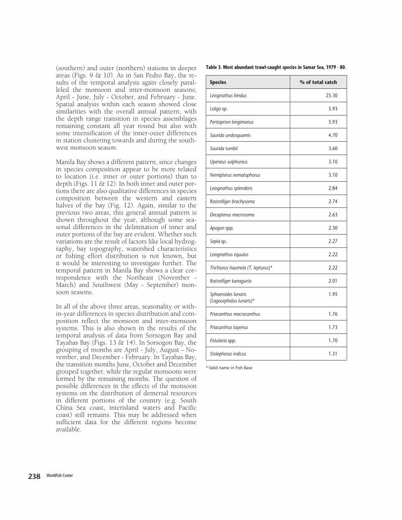
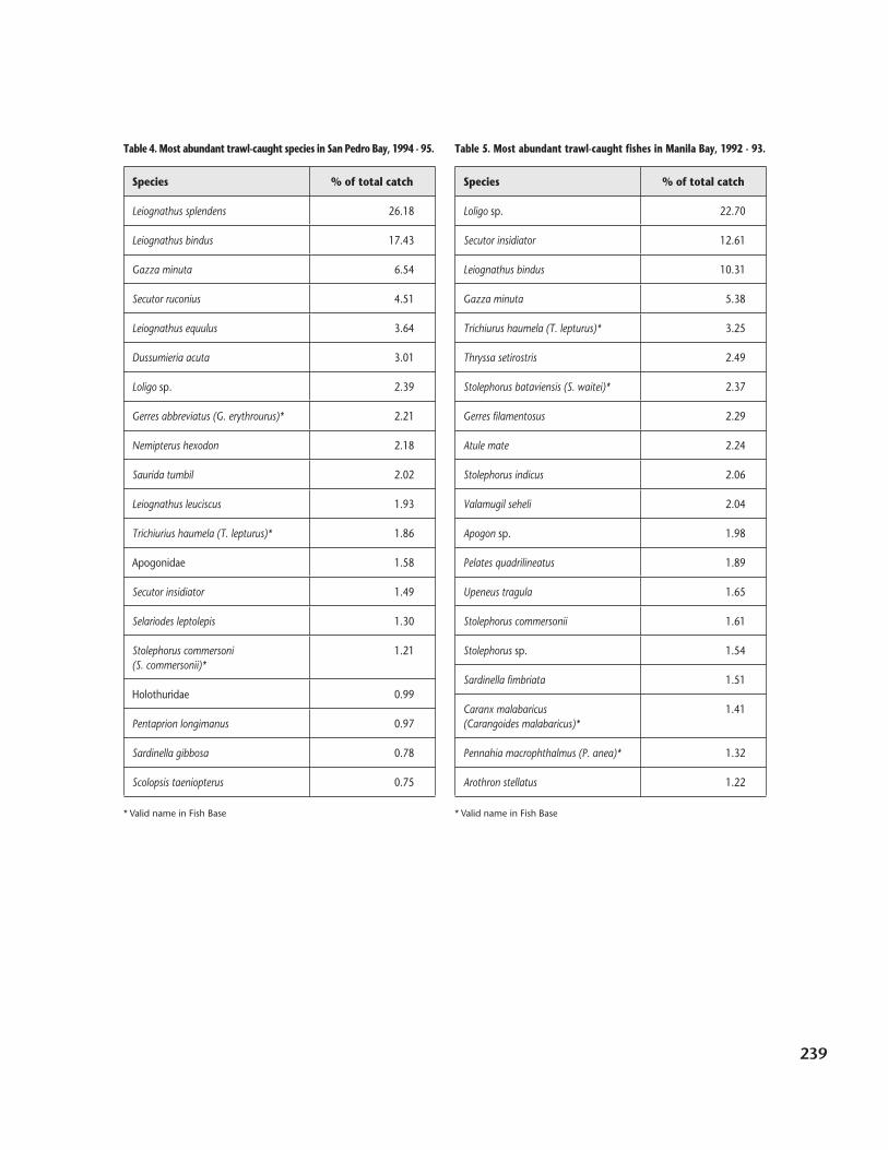
Generally, the demersal resources in Manila Bay, San Pedro Bay and Samar Sea are characterized by a large number of ubiquitous species that occur in varying abundances across the different habitats in the areas surveyed. In all three areas leiognathids comprised at least 28% of the total trawl catches, and together with squid (Loligo spp) comprised up to 59% of the total catch (Tables 3 - 5).

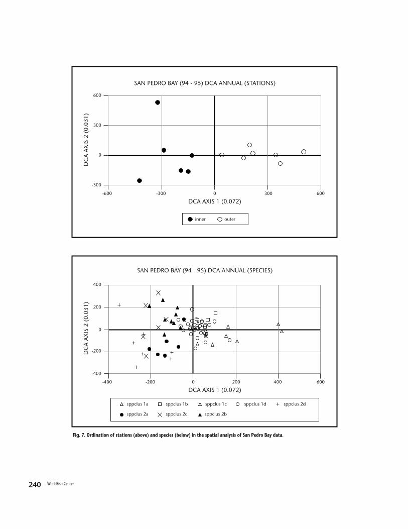
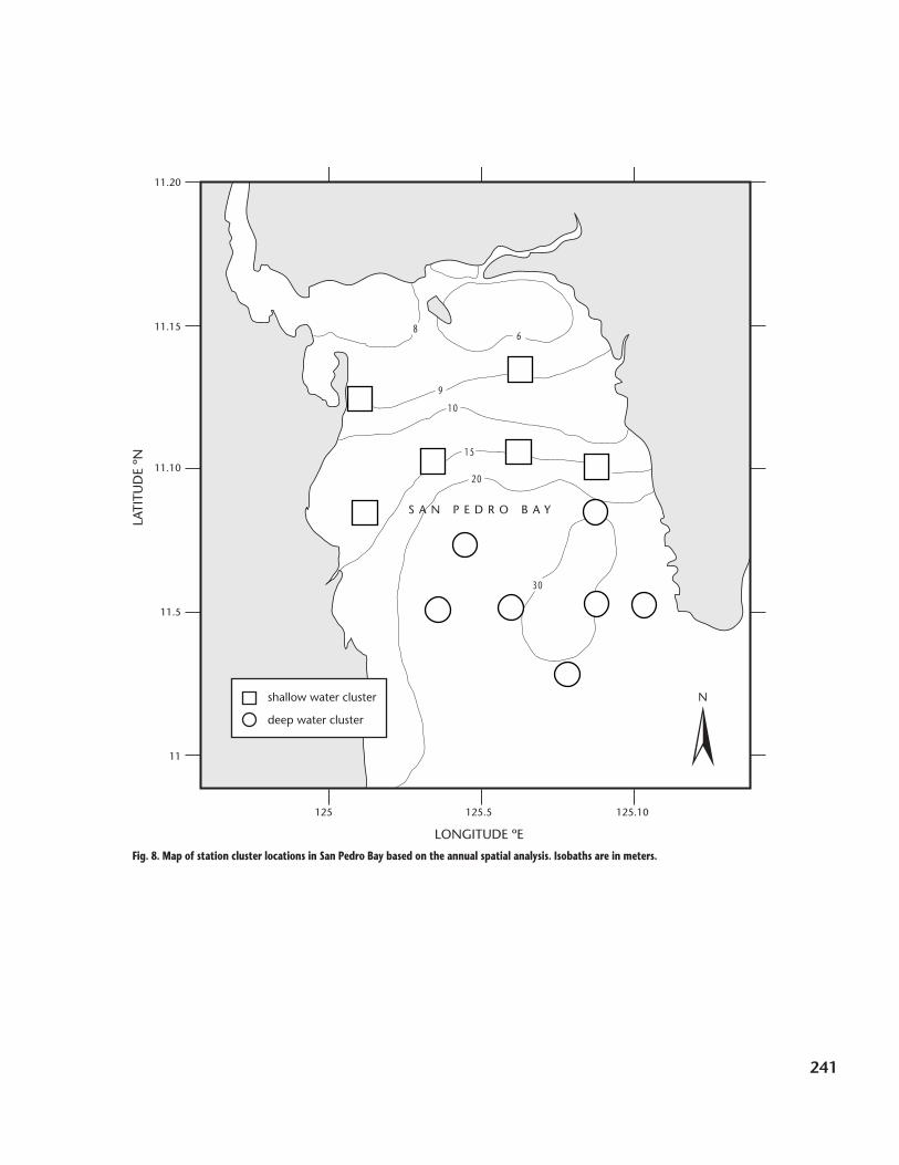
In terms of habitat relations, depth appears to be the primary factor in San Pedro Bay and Samar Sea. In San Pedro Bay, catch species composition shows a transition at depths of 15 - 20 m (Figs. 7 & 8).

This depth range transition is also consistent thr-oughout the year. Temporal analysis of the data showed the following grouping of months: June - July, August - November, and December - May; roughly corresponding to the monsoon and inter-monsoon seasons. The spatial distributions of sta-tion clusters during the SW monsoon and inter-monsoon seasons show little variation from the overall annual pattern (Fig. 8), particularly the tran-sition in species assemblage distribution at the 15 - 20 m depth range.

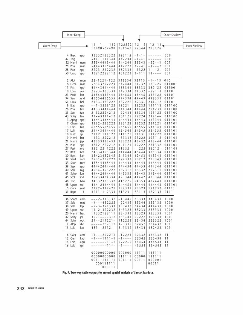
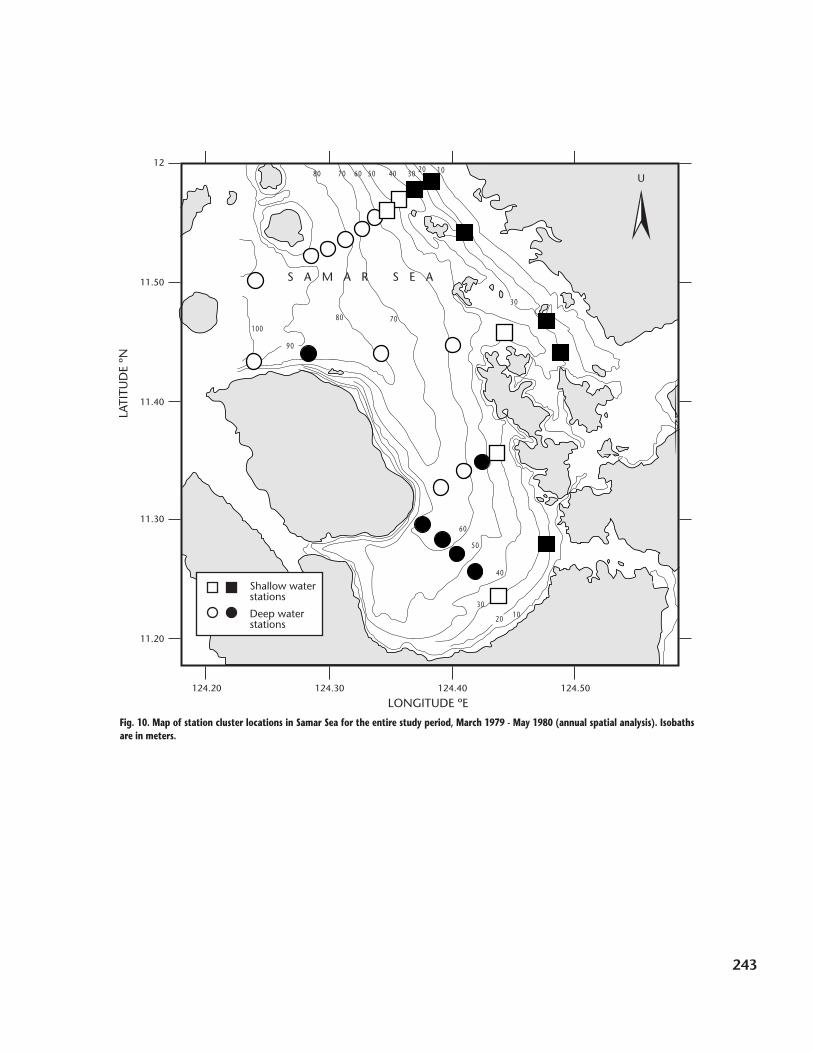
Similarly, demersal assemblage composition in Samar Sea shows a transition at the 30 - 40 m depth range, and again at the depths of 50 - 60 m, with further differences in composition between inner


Table 3. Most abundant trawl-caught species in Samar Sea, 1979 - 80.

Species % of total catch

Leiognathus bindus 25.30

Loligo sp. 5.93

Pentaprion longimanus 5.93

Saurida undosquamis 4.70

Saurida tumbil 3.60

Upeneus sulphureus 3.10

Nemipterus nematophorus 3.10

Leiognathus splendens 2.84

Rastrelliger brachysoma 2.74

Decapterus macrosoma 2.63

Apogon spp. 2.30

Sepia sp. 2.27

Leiognathus equulus 2.22

Trichiurus haumela (T. lepturus)* 2.22

Rastrelliger kanagurta 2.01

Sphoeroides lunaris(Lagocephalus lunaris)*

1.95

Priacanthus macracanthus 1.76

Priacanthus tayenus 1.73

Fistularia spp. 1.70

Stolephorus indicus 1.31

* Valid name in Fish Base

(southern) and outer (northern) stations in deeper areas (Figs. 9 & 10). As in San Pedro Bay, the re-sults of the temporal analysis again closely paral-leled the monsoon and inter-monsoon seasons; April - June, July - October, and February - June. Spatial analysis within each season showed close similarities with the overall annual pattern, with the depth range transition in species assemblages remaining constant all year round but also with some intensification of the inner-outer differences in station clustering towards and during the south-west monsoon season.

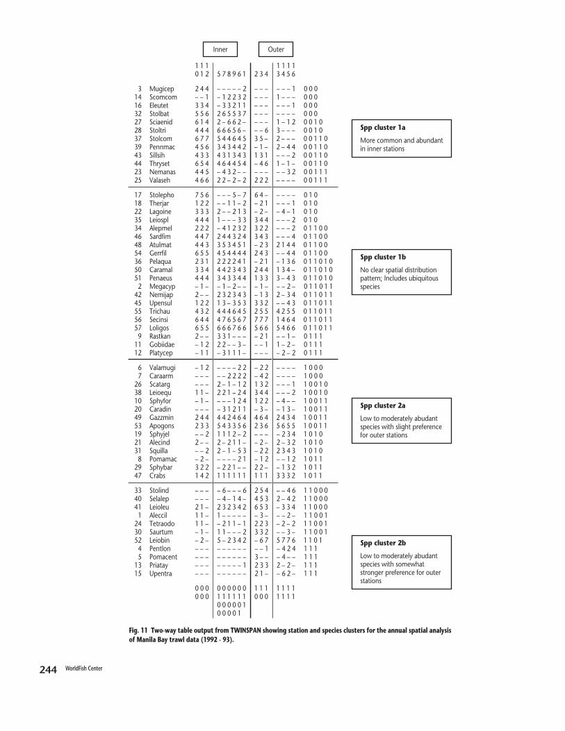
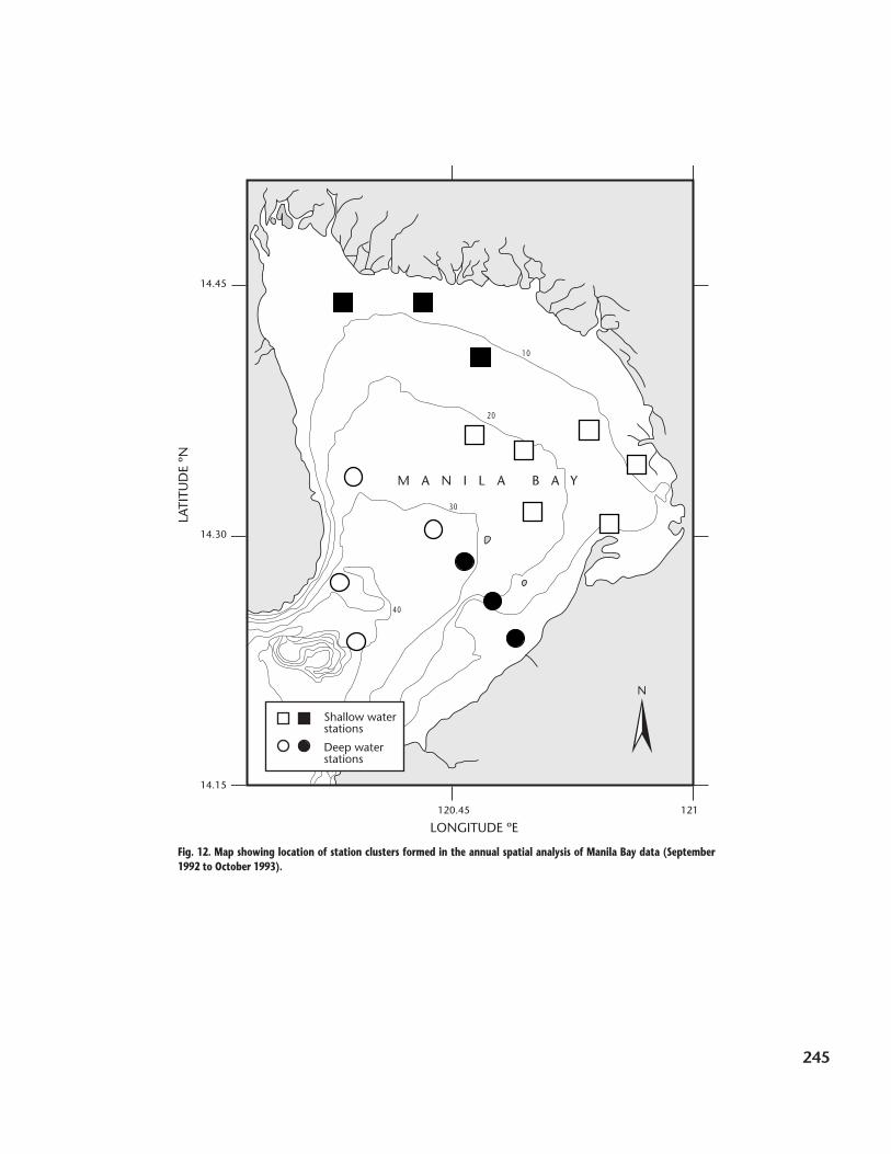
Manila Bay shows a different pattern, since changes in species composition appear to be more related to location (i.e. inner or outer portions) than to depth (Figs. 11 & 12). In both inner and outer por-tions there are also qualitative differences in species composition between the western and eastern halves of the bay (Fig. 12). Again, similar to the previous two areas, this general annual pattern is shown throughout the year, although some sea-sonal differences in the delimitation of inner and outer portions of the bay are evident. Whether such variations are the result of factors like local hydrog-raphy, bay topography, watershed characteristics or fishing effort distribution is not known, but it would be interesting to investigate further. The temporal pattern in Manila Bay shows a clear cor-respondence with the Northeast (November - March) and Southwest (May - September) mon-soon seasons.

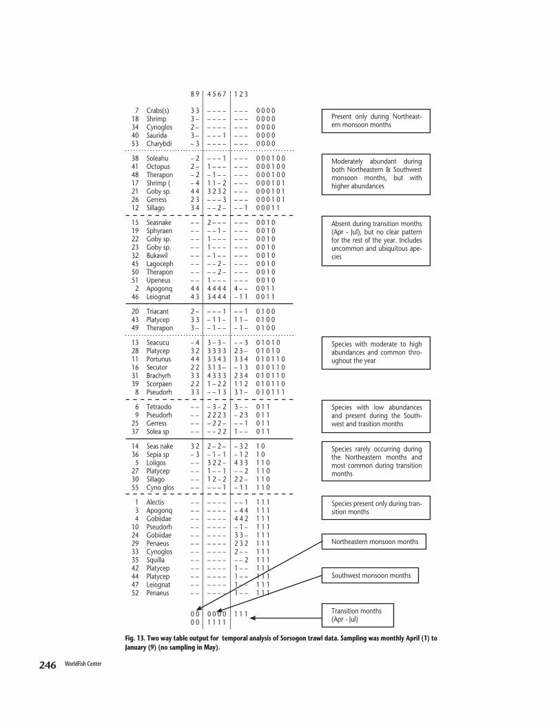
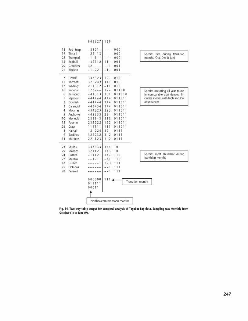
In all of the above three areas, seasonality or with-in-year differences in species distribution and com-position reflect the monsoon and inter-monsoon systems. This is also shown in the results of the temporal analysis of data from Sorsogon Bay and Tayabas Bay (Figs. 13 & 14). In Sorsogon Bay, the grouping of months are April - July, August - No-vember, and December - February. In Tayabas Bay, the transition months June, October and December grouped together, while the regular monsoons were formed by the remaining months. The question of possible differences in the effects of the monsoon systems on the distribution of demersal resources in different portions of the country (e.g. South China Sea coast, interisland waters and Pacific coast) still remains. This may be addressed when sufficient data for the different regions become available.


Table 4. Most abundant trawl-caught species in San Pedro Bay, 1994 - 95.


Leiognathus splendens 26.18


Gazza minuta 6.54

Secutor ruconius 4.51

Leiognathus equulus 3.64

Dussumieria acuta 3.01

Loligo sp. 2.39

Gerres abbreviatus (G. erythrourus)* 2.21

Nemipterus hexodon 2.18

Saurida tumbil 2.02

Leiognathus leuciscus 1.93

Trichiurius haumela (T. lepturus)* 1.86

Apogonidae 1.58

Secutor insidiator 1.49

Selariodes leptolepis 1.30

Stolephorus commersoni (S. commersonii)*

1.21

Holothuridae 0.99

Pentaprion longimanus 0.97

Sardinella gibbosa 0.78

Scolopsis taeniopterus 0.75


Table 5. Most abundant trawl-caught fishes in Manila Bay, 1992 - 93.


Loligo sp. 22.70

Secutor insidiator 12.61


Gazza minuta 5.38

Trichiurus haumela (T. lepturus)* 3.25

Thryssa setirostris 2.49

Stolephorus bataviensis (S. waitei)* 2.37

Gerres filamentosus 2.29

Atule mate 2.24

Stolephorus indicus 2.06

Valamugil seheli 2.04

Apogon sp. 1.98

Pelates quadrilineatus 1.89

Upeneus tragula 1.65

Stolephorus commersonii 1.61

Stolephorus sp. 1.54

Sardinella fimbriata 1.51

Caranx malabaricus (Carangoides malabaricus)*

1.41

Pennahia macrophthalmus (P. anea)* 1.32

Arothron stellatus 1.22



Fig. 7. Ordination of stations (above) and species (below) in the spatial analysis of San Pedro Bay data.

SAN PEDRO BAY (94 - 95) DCA ANNUAL (STATIONS)

-600 -300 0 300 600

600

300

0

-300

DC

A A

XIS

2 (

0.03

1)

DCA AXIS 1 (0.072)

inner outer

SAN PEDRO BAY (94 - 95) DCA ANNUAL (SPECIES)

-400 -200 0 200 400 600

400

200

0

-200

-400

DC

A A

XIS

2 (

0.03

1)

DCA AXIS 1 (0.072)

sppclus 1a sppclus 1b sppclus 1c sppclus 1d sppclus 2d

sppclus 2a sppclus 2c sppclus 2b


Fig. 8. Map of station cluster locations in San Pedro Bay based on the annual spatial analysis. Isobaths are in meters.

125 125.5 125.10

86

9

10

15

20

30

LATI

TUD

E ºN

11.20

11.15

11.10

11.5

11

LONGITUDE ºE

S A N P E D R O B A Y

Nshallow water cluster

deep water cluster


Fig. 9. Two-way table output for annual spatial analysis of Samar Sea data.

1 1 1 1 1 2 1 2 2 2 2 2 1 2 2 1 2 1 1 1 3 8 9 0 5 6 7 4 9 0 2 8 1 5 6 7 5 2 3 4 4 2 8 3 1 7 6 4 Brac spp 3 3 3 3 2 1 2 2 3 2 2 3 2 2 1 1 2 – 1 – 1 – – – – – – – 0 0 0 47 Trig 5 4 1 1 1 1 1 1 3 4 4 4 4 2 2 3 4 – 1 – – 1 – – – – – – 0 0 0 22 Nemi nem 5 5 5 4 4 4 4 5 4 4 4 5 4 4 2 4 4 2 3 3 4 3 – 2 2 – – 1 0 0 1 25 Pria mac 5 4 4 4 3 3 5 5 4 4 4 4 4 2 2 2 3 3 2 – 4 1 – 1 – – – 2 0 0 1 28 Pter spp 2 2 2 3 – 2 1 2 2 3 2 3 3 2 3 3 3 – 1 3 2 2 1 – – – 2 – 0 0 1 50 Urab spp 3 3 2 1 2 2 2 2 1 1 2 4 3 1 2 2 3 3 – 1 1 1 1 1 – – – – 0 0 1 2 Alut mon 2 2 – 1 2 2 1 – 1 2 2 3 3 3 3 3 4 3 2 1 1 3 – 1 – – 1 3 0 1 0 8 Deca mac 5 3 3 4 3 2 2 2 2 2 3 2 4 2 4 4 4 2 1 – 3 2 1 3 3 – 2 5 0 1 1 0 0 11 Fist spp 4 4 4 4 3 4 4 4 4 4 4 4 5 3 3 4 4 3 3 3 3 3 3 3 2 – 2 2 0 1 1 0 0 10 Epin sex 2 2 2 3 – 3 3 3 3 3 3 3 4 2 3 3 4 3 1 3 3 2 – 2 2 1 1 3 0 1 1 0 1 23 Pent lon 5 4 5 5 4 4 3 3 4 4 4 5 5 4 5 5 5 4 5 4 4 5 3 3 3 1 2 2 0 1 1 0 1 34 Saur und 4 5 5 5 4 4 5 5 5 5 5 4 4 4 3 3 4 4 4 4 4 3 4 4 2 3 3 3 0 1 1 0 1 51 Uras hel 2 1 3 3 – 3 3 3 2 2 2 3 3 2 2 2 2 3 2 3 3 – 2 1 1 – 1 2 0 1 1 0 1 9 Elat spp – – 1 – 3 3 2 3 1 2 2 1 3 2 2 1 3 3 2 3 2 1 1 1 1 1 3 0 1 1 1 0 0 26 Pria tay 4 4 3 3 3 4 4 4 4 4 4 3 4 4 3 4 4 4 4 4 4 4 2 2 4 2 3 3 0 1 1 1 0 0 35 Scol tae 2 – 3 3 2 2 2 4 2 1 2 – 2 2 4 3 3 3 3 3 3 4 1 2 3 1 2 2 0 1 1 1 0 0 43 Sphy lan 3 1 – 4 3 3 1 1 – 1 2 2 3 1 1 2 2 1 2 2 2 4 2 1 2 1 – – 0 1 1 1 0 0 3 Apog spp 4 4 4 4 3 4 4 4 4 4 4 4 4 4 4 4 4 4 4 4 4 3 4 4 3 3 4 4 0 1 1 1 0 1 7 Cham spp 3 2 3 2 – 2 2 2 2 2 2 2 2 2 1 2 2 2 3 2 3 2 2 2 1 2 2 1 0 1 1 1 0 1 13 Leio bin 6 5 5 5 5 5 5 5 4 5 5 5 5 5 6 5 5 4 5 5 5 5 5 4 4 3 4 3 0 1 1 1 0 1 17 Loli spp 5 4 4 4 3 4 4 4 4 4 4 4 5 4 5 4 4 5 4 5 4 5 5 5 4 5 5 5 0 1 1 1 0 1 18 Natn sp 2 1 1 2 1 1 1 1 1 2 2 2 1 1 1 2 2 1 1 1 3 1 1 1 1 2 2 2 0 1 1 1 0 1 19 Nemi bat – 1 3 3 – 2 2 2 2 1 2 – 3 3 3 3 3 2 3 2 2 2 3 2 3 1 – 2 0 1 1 1 0 1 21 Nemi jap 4 3 3 3 3 3 3 3 4 3 3 3 3 3 2 2 3 4 3 4 3 2 4 3 3 4 4 4 0 1 1 1 0 1 24 Plat spp 3 3 1 2 1 2 2 2 2 1 2 4 – 1 1 2 1 1 2 2 2 2 2 3 1 3 3 2 0 1 1 1 0 1 27 Pset eru 3 2 2 – 2 2 – 1 2 2 2 3 1 3 3 2 – – 2 2 2 3 3 2 1 2 – 0 1 1 1 0 1 29 Rast bra 2 4 3 3 4 3 5 3 3 4 4 3 4 4 4 4 4 4 5 4 4 4 3 3 5 3 3 4 0 1 1 1 0 1 30 Rast kan 3 3 4 2 3 4 3 2 5 4 5 2 – 1 3 4 3 4 2 4 5 3 4 4 3 3 4 3 0 1 1 1 0 1 32 Sard sam 2 2 3 1 – 2 3 2 2 2 2 1 2 2 3 3 3 2 3 2 1 2 2 3 3 3 4 3 0 1 1 1 0 1 33 Saur tum 4 5 5 4 4 4 4 5 4 4 4 4 4 4 4 4 4 4 4 4 4 4 4 4 4 4 4 4 0 1 1 1 0 1 39 Sepi spp 4 4 4 4 2 4 4 4 4 4 4 4 4 4 4 3 4 4 4 4 5 3 4 4 4 3 4 4 0 1 1 1 0 1 40 Seri nig 4 2 3 4 – 3 2 3 2 2 2 3 3 2 3 1 2 1 3 3 3 2 2 2 2 3 1 1 0 1 1 1 0 1 41 Spho lun 4 4 4 4 2 4 4 4 4 4 4 4 4 3 3 3 3 4 3 4 4 3 3 4 3 4 4 4 0 1 1 1 0 1 45 Stol ind 3 2 2 3 3 4 3 4 3 3 4 4 2 3 3 4 4 4 4 4 4 2 4 3 3 3 4 4 0 1 1 1 0 1 46 Tric hau 3 4 3 3 2 3 3 3 3 3 2 4 1 5 2 2 5 5 4 3 5 3 4 3 2 4 4 3 0 1 1 1 0 1 48 Upen sul 4 4 4 – 2 4 4 4 4 4 4 5 4 4 4 5 4 3 4 4 4 4 4 4 4 4 4 3 0 1 1 1 0 1 5 Cara mal 2 1 2 2 – 3 1 2 – 2 1 3 3 2 3 3 2 2 3 3 2 3 1 2 1 2 3 2 0 1 1 1 1 31 Rept 3 3 2 1 1 – 1 – 2 3 3 3 3 1 3 2 3 3 3 1 1 3 1 3 2 1 3 3 0 1 1 1

36 Scom com – – – 2 – 3 1 3 1 3 2 – 1 3 4 4 2 3 3 3 3 3 3 4 3 4 3 3 1 0 0 0 37 Sela mat – 4 – – – 4 3 2 2 2 2 – 2 2 4 3 2 3 3 3 4 4 3 3 3 1 3 2 1 0 0 0 38 Sela lep – 2 – 3 – 3 2 1 3 3 3 1 3 3 4 3 3 3 4 4 3 4 4 4 4 4 3 3 1 0 0 0 49 Upen sun 1 1 – 2 – 3 2 2 2 3 2 3 4 3 3 2 3 3 3 2 3 3 2 3 3 3 3 3 1 0 0 0 20 Nemi hex 1 1 3 3 2 1 2 2 1 1 1 2 3 – 3 3 3 3 3 3 2 3 3 3 3 3 3 3 1 0 0 1 42 Sphy jel 3 2 – 1 – – – – 3 1 2 3 3 3 – 4 4 2 – 2 2 2 3 2 3 3 3 3 1 0 0 1 44 Sphy obt 2 1 – – 2 1 1 2 2 1 – 4 1 2 2 2 3 2 3 – 3 4 2 2 3 3 2 2 1 0 0 1 1 Alep dje – – – – – 2 3 – 1 1 2 1 – 3 3 3 2 3 2 4 5 2 2 3 4 4 3 2 1 0 1 15 Leio leu 4 3 1 – – 2 1 1 2 – – 3 – 1 3 3 2 4 3 4 3 4 4 3 2 4 2 3 1 0 1

6 Cara arm 1 1 – – – 2 2 2 2 1 1 – 1 2 2 2 1 2 2 3 3 2 3 3 3 3 3 2 1 1 12 Gerr kap – 1 – – – 1 1 1 1 – 1 – 1 – – – – 3 2 3 4 2 2 3 3 4 3 4 1 1 14 Leio equ – – – – – – – 1 1 – 2 2 2 2 2 – 2 4 4 4 5 4 4 4 4 5 4 4 1 1 16 Leio spl – – – – – – – 1 1 – – – 1 – – – – 4 3 5 5 3 3 5 4 5 4 5 1 1

0 0 0 0 0 0 0 0 0 0 0 0 0 0 0 0 0 1 1 1 1 1 1 1 1 1 1 1 0 0 0 0 0 0 0 0 0 0 0 1 1 1 1 1 1 0 0 0 0 0 1 1 1 1 1 1 0 0 1 1 1 1 1 1 1 1 1 0 0 1 1 1 1 0 0 1 1 1 0 0 0 0 0 1 0 0 0 1 1 1 1 1 1 0 0 0 1 1 0 0 0 1 1 1

Inner ShallowOuter Deep

Outer ShallowInner Deep


Fig. 10. Map of station cluster locations in Samar Sea for the entire study period, March 1979 - May 1980 (annual spatial analysis). Isobaths are in meters.

80

100

90

80 70

20

30

40

50

60

10

70 60 50 40 30

30

20 10

LATI

TUD

E ºN

124.20 124.30 124.40 124.50

12

11.50

11.40

11.30

11.20

LONGITUDE ºE

U

S A M A R S E A

Shallow water stations

Deep water stations


Fig. 11 Two-way table output from TWINSPAN showing station and species clusters for the annual spatial analysis of Manila Bay trawl data (1992 - 93).

1 1 1 1 1 1 1 0 1 2 5 7 8 9 6 1 2 3 4 3 4 5 6 3 Mugicep 2 4 4 – – – – – 2 – – – – – – 1 0 0 0 14 Scomcom – – 1 – 1 2 2 3 2 – – – 1 – – – 0 0 0 16 Eleutet 3 3 4 – 3 3 2 1 1 – – – – – – 1 0 0 0 32 Stolbat 5 5 6 2 6 5 5 3 7 – – – – – – – 0 0 0 27 Sciaenid 6 1 4 2 – 6 6 2 – – – – 1 – 1 2 0 0 1 0 28 Stoltri 4 4 4 6 6 6 5 6 – – – 6 3 – – – 0 0 1 0 37 Stolcom 6 7 7 5 4 4 6 4 5 3 5 – 2 – – – 0 0 1 1 0 39 Pennmac 4 5 6 3 4 3 4 4 2 – 1 – 2 – 4 4 0 0 1 1 0 43 Sillsih 4 3 3 4 3 1 3 4 3 1 3 1 – – – 2 0 0 1 1 0 44 Thryset 6 5 4 4 6 4 4 5 4 – 4 6 1 – 1 – 0 0 1 1 0 23 Nemanas 4 4 5 – 4 3 2 – – – – – – – 3 2 0 0 1 1 1 25 Valaseh 4 6 6 2 2 – 2 – 2 2 2 2 – – – – 0 0 1 1 1

17 Stolepho 7 5 6 – – – 5 – 7 6 4 – – – – – 0 1 0 18 Therjar 1 2 2 – – 1 1 – 2 – 2 1 – – – 1 0 1 0 22 Lagoine 3 3 3 2 – – 2 1 3 – 2 – – 4 – 1 0 1 0 35 Leiospl 4 4 4 1 – – – 3 3 3 4 4 – – – 2 0 1 0 34 Alepmel 2 2 2 – 4 1 2 3 2 3 2 2 – – – 2 0 1 1 0 0 46 Sardfim 4 4 7 2 4 4 3 2 4 3 4 3 – – – 4 0 1 1 0 0 48 Atulmat 4 4 3 3 5 3 4 5 1 – 2 3 2 1 4 4 0 1 1 0 0 54 Gerrfil 6 5 5 4 5 4 4 4 4 2 4 3 – – 4 4 0 1 1 0 0 36 Pelaqua 2 3 1 2 2 2 2 4 1 – 2 1 – 1 3 6 0 1 1 0 1 0 50 Caramal 3 3 4 4 4 2 3 4 3 2 4 4 1 3 4 – 0 1 1 0 1 0 51 Penaeus 4 4 4 3 4 3 3 4 4 1 3 3 3 – 4 3 0 1 1 0 1 0 2 Megacyp – 1 – – 1 – 2 – – – 1 – – – 2 – 0 1 1 0 1 1 42 Nemijap 2 – – 2 3 2 3 4 3 – 1 3 2 – 3 4 0 1 1 0 1 1 45 Upensul 1 2 2 1 3 – 3 5 3 3 3 2 – – 4 3 0 1 1 0 1 1 55 Trichau 4 3 2 4 4 4 6 4 5 2 5 5 4 2 5 5 0 1 1 0 1 1 56 Secinsi 6 4 4 4 7 6 5 6 7 7 7 7 1 4 6 4 0 1 1 0 1 1 57 Loligos 6 5 5 6 6 6 7 6 6 5 6 6 5 4 6 6 0 1 1 0 1 1 9 Rastkan 2 – – 3 3 1 – – – – 2 1 – – 1 – 0 1 1 1 11 Gobiidae – 1 2 2 2 – – 3 – – – 1 1 – 2 – 0 1 1 1 12 Platycep – 1 1 – 3 1 1 1 – – – – – 2 – 2 0 1 1 1

6 Valamugi – 1 2 – – – – 2 2 – 2 2 – – – – 1 0 0 0 7 Caraarm – – – – – 2 2 2 2 – 4 2 – – – – 1 0 0 0 26 Scatarg – – – 2 – 1 – 1 2 1 3 2 – – – 1 1 0 0 1 0 38 Leioequ 1 1 – 2 2 1 – 2 4 3 4 4 – – – 2 1 0 0 1 0 10 Sphyfor – 1 – – – – 1 2 4 1 2 2 – 4 – – 1 0 0 1 1 20 Caradin – – – – 3 1 2 1 1 – 3 – – 1 3 – 1 0 0 1 1 49 Gazzmin 2 4 4 4 4 2 4 6 4 4 6 4 2 4 3 4 1 0 0 1 1 53 Apogons 2 3 3 5 4 3 3 5 6 2 3 6 5 6 5 5 1 0 0 1 1 19 Sphyjel – – 2 1 1 1 2 – 2 – – – – 2 3 4 1 0 1 0 21 Alecind 2 – – 2 – 2 1 1 – – 2 – 2 – 3 2 1 0 1 0 31 Squilla – – 2 2 – 1 – 5 3 – 2 2 2 3 4 3 1 0 1 0 8 Pomamac – 2 – – – – – 2 1 – 1 2 – – 1 2 1 0 1 1 29 Sphybar 3 2 2 – 2 2 1 – – 2 2 – – 1 3 2 1 0 1 1 47 Crabs 1 4 2 1 1 1 1 1 1 1 1 1 3 3 3 2 1 0 1 1

33 Stolind – – – – 6 – – – 6 2 5 4 – – 4 6 1 1 0 0 0 40 Selalep – – – – 4 – 1 4 – 4 5 3 2 – 4 2 1 1 0 0 0 41 Leioleu 2 1 – 2 3 2 3 4 2 6 5 3 – 3 3 4 1 1 0 0 0 1 Aleccil 1 1 – 1 – – – – – – 3 – – – 2 – 1 1 0 0 1 24 Tetraodo 1 1 – – 2 1 1 – 1 2 2 3 – 2 – 2 1 1 0 0 1 30 Saurtum – 1 – 1 1 – – – 2 3 3 2 – – 3 – 1 1 0 0 1 52 Leiobin – 2 – 5 – 2 3 4 2 – 6 7 5 7 7 6 1 1 0 1 4 Pentlon – – – – – – – – – – – 1 – 4 2 4 1 1 1 5 Pomacent – – – – – – – – – 3 – – – 4 – – 1 1 1 13 Priatay – – – – – – – – 1 2 3 3 2 – 2 – 1 1 1 15 Upentra – – – – – – – – – 2 1 – – 6 2 – 1 1 1

0 0 0 0 0 0 0 0 0 1 1 1 1 1 1 1 0 0 0 1 1 1 1 1 1 0 0 0 1 1 1 1 0 0 0 0 0 1 0 0 0 0 1

Spp cluster 1a

More common and abundantin inner stations

Spp cluster 1b

No clear spatial distribution pattern; Includes ubiquitous species

Spp cluster 2a

Low to moderately abudant species with slight preference for outer stations

Spp cluster 2b

Low to moderately abudant species with somewhat stronger preference for outer stations

OuterInner


Fig. 12. Map showing location of station clusters formed in the annual spatial analysis of Manila Bay data (September 1992 to October 1993).

10

20

30

40

LATI

TUD

E ºN

120.45 121

14.45

14.30

14.15

LONGITUDE ºE

N

M A N I L A B A Y

Shallow water stations

Deep water stations


Fig. 13. Two way table output for temporal analysis of Sorsogon trawl data. Sampling was monthly April (1) to January (9) (no sampling in May).

8 9 4 5 6 7 1 2 3 7 Crabs(s) 3 3 – – – – – – – 0 0 0 0 18 Shrimp 3 – – – – – – – – 0 0 0 0 34 Cynoglos 2 – – – – – – – – 0 0 0 0 40 Saurida 3 – – – – 1 – – – 0 0 0 0 53 Charybdi – 3 – – – – – – – 0 0 0 0 38 Soleahu – 2 – – – 1 – – – 0 0 0 1 0 0 41 Octopus 2 – 1 – – – – – – 0 0 0 1 0 0 48 Therapon – 2 – 1 – – – – – 0 0 0 1 0 0 17 Shrimp ( – 4 1 1 – 2 – – – 0 0 0 1 0 1 21 Goby sp. 4 4 3 2 3 2 – – – 0 0 0 1 0 1 26 Gerress 2 3 – – – 3 – – – 0 0 0 1 0 1 12 Sillago 3 4 – – 2 – – – 1 0 0 0 1 1 15 Seasnake – – 2 – – – – – – 0 0 1 0 19 Sphyraen – – – – 1 – – – – 0 0 1 0 22 Goby sp. – – 1 – – – – – – 0 0 1 0 23 Goby sp. – – 1 – – – – – – 0 0 1 0 32 Bukawil – – – 1 – – – – – 0 0 1 0 45 Lagoceph – – – – 2 – – – – 0 0 1 0 50 Therapon – – – – 2 – – – – 0 0 1 0 51 Upeneus – – 1 – – – – – – 0 0 1 0 2 Apogonq 4 4 4 4 4 4 4 – – 0 0 1 1 46 Leiognat 4 3 3 4 4 4 – 1 1 0 0 1 1 20 Triacant 2 – – – – 1 – – 1 0 1 0 0 43 Platycep 3 3 – 1 1 – 1 1 – 0 1 0 0 49 Therapon 3 – – 1 – – – 1 – 0 1 0 0 13 Seacucu – 4 3 – 3 – – – 3 0 1 0 1 0 28 Platycep 3 2 3 3 3 3 2 3 – 0 1 0 1 0 11 Portunus 4 4 3 3 4 3 3 3 4 0 1 0 1 1 0 16 Secutor 2 2 3 1 3 – – 1 3 0 1 0 1 1 0 31 Brachyrh 3 3 4 3 3 3 2 3 4 0 1 0 1 1 0 39 Scorpaen 2 2 1 – 2 2 1 1 2 0 1 0 1 1 0 8 Pseudorh 3 3 – – 1 3 3 1 – 0 1 0 1 1 1 6 Tetraodo – – – 3 – 2 3 – – 0 1 1 9 Pseudorh – – 2 2 2 3 – 2 3 0 1 1 25 Gerress – – – 2 2 – – – 1 0 1 1 37 Solea sp – – – – 2 2 1 – – 0 1 1 14 Seas nake 3 2 2 – 2 – – 3 2 1 0 36 Sepia sp – 3 – 1 – 1 – 1 2 1 0 5 Loligos – – 3 2 2 – 4 3 3 1 1 0 27 Platycep – – 1 – – 1 – – 2 1 1 0 30 Sillago – – 1 2 – 2 2 2 – 1 1 0 55 Cyno glos – – – – – 1 – 1 1 1 1 0 1 Alectis – – – – – – – – 1 1 1 1 3 Apogonq – – – – – – – 4 4 1 1 1 4 Gobiidae – – – – – – 4 4 2 1 1 1 10 Pseudorh – – – – – – – 1 – 1 1 1 24 Gobiidae – – – – – – 3 3 – 1 1 1 29 Penaeus – – – – – – 2 3 2 1 1 1 33 Cynoglos – – – – – – 2 – – 1 1 1 35 Squilla – – – – – – – – 2 1 1 1 42 Platycep – – – – – – 1 – – 1 1 1 44 Platycep – – – – – – 1 – – 1 1 1 47 Leiognat – – – – – – 1 – – 1 1 1 52 Penaeus – – – – – – 1 – – 1 1 1

0 0 0 0 0 0 1 1 1 0 0 1 1 1 1

Present only during Northeast-ern monsoon months

Moderately abundant during both Northeastern & Southwest monsoon months, but with higher abundances

Absent during transition months (Apr - Jul), but no clear pattern for the rest of the year. Includes uncommon and ubiquitous ape-cies

Species with moderate to high abundances and common thro-ughout the year

Species with low abundances and present during the South-west and trasition months

Species rarely occurring during the Northeastern months and most common during transition months

Species present only during tran-sition months

Northeastern monsoon months

Southwest monsoon months

Transition months(Apr - Jul)


Fig. 14. Two way table output for temporal analysis of Tayabas Bay data. Sampling was monthly from October (1) to June (9).

8 4 5 6 2 7 1 3 9 13 Red Snap – 3 3 2 1 – – – – 0 0 0 19 Thick-li – 2 2 – 1 3 – – – 0 0 0 22 Trumpetf – 1 – 1 – – – – – 0 0 0 15 Redbull – 3 2 3 1 2 1 1 – 0 0 1 20 Groupers 3 2 – – – – – – 1 0 0 1 21 Blackpo – 1 – 2 2 1 – 1 – 0 0 1 7 Lizardfi 3 4 3 3 2 3 1 2 – 0 1 0 11 Threadfi 3 2 3 2 4 3 1 1 1 0 1 0 17 Whitings 2 1 1 3 1 2 – 1 1 0 1 0 16 Imperial 1 2 3 2 – – 1 2 – 0 1 1 0 0 6 Barracud – 4 1 3 1 3 3 3 1 0 1 1 0 1 0 1 Slipmout 4 4 4 4 4 4 4 4 4 0 1 1 0 1 1 2 Goatfish 4 4 4 4 4 4 3 4 4 0 1 1 0 1 1 3 Carangid 4 4 3 4 3 4 3 4 4 0 1 1 0 1 1 4 Mojarras 4 3 4 3 2 3 2 2 3 0 1 1 0 1 1 5 Anchovie 4 4 2 3 3 3 2 2 – 0 1 1 0 1 1 10 Monocle 2 3 3 3 – 3 2 1 3 0 1 1 0 1 1 12 Four-lin 2 3 2 2 2 2 1 2 2 0 1 1 0 1 1 26 Crabs 1 1 1 1 1 1 1 1 1 0 1 1 0 1 1 8 Hairtail – 2 – 2 2 4 3 2 – 0 1 1 1 9 Sardines 3 2 2 2 3 2 3 – 2 0 1 1 1 14 Mackerel 2 2 – 1 2 3 1 – 2 0 1 1 1 23 Squids 3 3 3 3 3 3 3 4 4 1 0 29 Scallops 3 2 1 1 2 1 1 4 3 1 0 24 Cuttlefi – 1 1 1 2 1 1 4 – 1 1 0 27 Mantiss – – 1 – 1 1 – 4 1 1 1 0 18 Fusilier – – – – – 1 2 – 3 1 1 1 25 Octopus – – – – – – – – 1 1 1 1 28 Penaeid – – – – – – – – 1 1 1 1 0 0 0 0 0 0 1 1 1 0 1 1 1 1 1 0 0 0 1 1

Species rare during transition months (Oct, Dec & Jun)

Species occurring all year round in comparable abundances. In-cludes species with high and low abundances

Species most abundant during transition months

Transition months

Northeastern monsoon months

248 WorldFish Center

Conclusion

The 24 fishing grounds in the exploratory surveys in 1947 - 49 can be arranged in gradients reflecting their substrate make-up (i.e. relative coral cover and sediment characteristics). Catch rate (kg.hr-1) was negatively correlated with both average water depth (-0.48, p < 0.05) and mud/sand substrate(-0.51, p < 0.05), and reflects an underlying trend of increasing catch rates in areas with shallower and more muddy bottoms. This is also consistent with the distribution of the more abundant families in the catches (e.g. Leiognathidae, Mullidae).

Depth appears to be the primary factor that deter-mines the station clusters in Samar Sea and San Pedro Bay. In San Pedro Bay, catch species compo-sition shows a consistent transition at depths of 15 - 20 m throughout the year. Similarly, Samar Sea shows a transition at the 30 - 40 m depth range, and again at the depths of 50 - 60 m, with further differences in composition between inner (southern) and outer (northern) stations. Manila Bay shows a different pattern; changes in species composition appear to be more related to location (i.e. inner or outer portions) than to depth. Differences in de-mersal assemblages were observed throughout the year in both inner and outer portions, and between the western and eastern halves of the bay seasonality or within-year differences in species assemblages reflecting the monsoon systems were also evident in Sorsogon Bay and Tayabas Bay.

References

Armada, N.B. 1996. The fisheries of San Pedro Bay, Philippines. Volume 5. Resource and Ecological Assessment of San Pedro Bay, Philippines. IMFO Technical Report No. 16. Institute of Marine Fisheries and Oceanography, College of Fisheries, UP Visayas, Miagao, Iloilo, Philippine.

Armada, N.B., C. Hammer, J. Saeger and G.T. Silvestre. 1983. Results of the Samar Sea trawl survey, p. 1 - 46. In J. Saeger, ed. Technical reports of the Department of Marine Fisheries No. 3. College of Fisheries, UP in the Visayas and GTZ, Republic of Germany. p 191.

Cinco, E. and L. Perez. 1996. Results of the Sorsogon Bay trawl survey, In E. Cinco et al. (eds.) Resource and Ecological Assessment of Sorsogon Bay, Volume III. Final Reports. UB Tech, Incorporated and FSP-Department of Agriculture.

Hill, M.O. 1979. TWINSPAN-a FORTRAN program for arranging multivariate data in an ordered two-way table by classification of the individuals and attributes. Section of Ecology and Systematics, Cornell University, Ithaca, New York.

MADECOR (Mandala Agricultural Development Corporation) and National Museum. 1995. Fisheries Sector Program- Resource and ecological assessment of the Manila Bay. Final Report.

Resources Combines Incorporated. 1997. Introduction and assessment of fishery resources (volume 1). resource and ecological assessment of Tayabas Bay. Fisheries Sector Program, Department of Agriculture, Quezon City.

Ter Braak, C.J. 1988. CANOCO-A FORTRAN program for canonical community ordination by partial detrended canonical correspondence analysis, principal components analysis and redundancy analysis (Version 2.1). Agricultural Mathematics Group, Wageningen, The Netherlands.

Warfel, H., and P. Manacorp. 1950. Otter trawl explorations in Philippines waters. Research Report 25, Fish and Wildlife Service. US Department of the Interior, Washing, D.C., USA.

Documents

Analysis of Demersal Fish Assemblages in Selected ...pubs.iclarm.net/resource_centre/AMF_Chapter-11-FA.pdf · Analysis of Demersal Fish Assemblages in Selected Philippine Fishing